MaxEnt-Copula-Oct2020
Abstract
A new nonparametric model of maximum-entropy (MaxEnt) copula density function is proposed, which offers the following advantages: (i) it is valid for mixed random vector. By ‘mixed’ we mean the method works for any combination of discrete or continuous variables in a fully automated manner; (ii) it yields a bonafide density estimate with intepretable parameters. By ‘bonafide’ we mean the estimate guarantees to be a non-negative function, integrates to ; and (iii) it plays a unifying role in our understanding of a large class of statistical methods for mixed . Our approach utilizes modern machinery of nonparametric statistics to represent and approximate log-copula density function via LP-Fourier transform. Several real-data examples are also provided to explore the key theoretical and practical implications of the theory.
A Maximum Entropy Copula Model for Mixed Data:
Representation, Estimation, and Applications
Deep Mukhopadhyay
deep@unitedstatalgo.com
Final Version: August, 2022
Keywords: Maximum entropy; Self-adaptive copula model; LP-Fourier transform; Categorical data analysis; Copula-logistic regression; United Statistical learning.
1 Copula Statistical Learning
Copulas are the ‘bridge’ between the univariate and the multivariate statistics world, with applications in a wide variety of science and engineering fields—from economics to finance to marketing to healthcare. Because of the ubiquity of copula in empirical research, it is becoming necessary to develop a general theory that can unify and simplify the copula learning process. In this paper, we present a new class specially-designed nonparametric maximum-entropy (MaxEnt) copula model that offers the following advantages: First, it yields a bonafide (smooth, non-negative, and integrates to ) copula density estimate with interpretable parameters that provide insights into the nature of the dependence between the random variables . Secondly, the method is data-type agnostic—which is to say that it automatically (self) adapts to mixed-data types (any combination of discrete, continuous, or even categorical). Thirdly, and most notably, our copula-theoretic framework subsumes and unifies a wide range of statistical learning methods using a common mathematical notation—unlocking deep, surprising connections and insights, which were previously unknown. In the development of our theory and algorithms, the LP-Fourier method of copula modeling (which was initiated by Mukhopadhyay and Parzen 2020), plays an indispensable role.
2 Self-Adaptive Nonparametric Models
We introduce two new classes of maximum-entropy (MaxEnt) copula density models. But before diving into technical details, it will be instructive to review some basic definitions and concepts related to copula.
2.1 Background Concepts and Notation
Sklar’s Copula Representation Theory (Sklar 1959). The joint cumulative distribution function (cdf) of any pair of random variables
can be decomposed as a function of the marginal cdfs and
| (2.1) |
where denotes a copula distribution function with uniform marginals. To set the stage, we start with the continuous marginals case, which will be generalized later to allow mixed-. Taking derivative of Eq. (2.1), we get
| (2.2) |
which decouples the joint density into the marginals and the copula. One can rewrite Eq. (2.2) to represent copula as a “normalized” joint density function
| (2.3) |
which is also known as the dependence function, pioneered by Hoeffding 1940. To make (2.3) a proper density function (i.e., one that integrates to one) we perform quantile transformation by substituting :
We are now ready to extend this copula density concept to the mixed case.
Pre-Copula: Conditional Comparison Density (Parzen and Mukhopadhyay 2013). Before we introduce the generalized copula density, we need to introduce a new concept—conditional comparison density (CCD). For a continuous , CCD is defined as:
| (2.4) |
For discrete, we represent it using probability mass function (pmf):
| (2.5) |
where is the quantile function of . It is easy to see that the CCDs (2.4) and (2.5) are proper densities in the sense that
Generalized Copula Representation Theory (Mukhopadhyay and Parzen 2020). For the mixed case, when is discrete and is continuous the joint density of (2.3) is defined by either side of the following identity:
This can be rewritten as the ratios of conditionals and their respective marginals:
| (2.6) |
This formula (2.6) can be interpreted as the slices of the mixed copula density, since
| (2.7) |
Substituting and , we get the following definition of the generalized copula density in terms of conditional comparison density (CCD):
| (2.8) |
Bayes’ theorem ensures the equality of two CCDs, with copula being the common value. Equipped with this fundamentals, we now develop the nonparametric theory of MaxEnt copula modeling.
2.2 Log-bilinear Model
An exponential Fourier series representation of copula density function is given. The reasons for entertaining an exponential model for copula is motivated from two different perspectives.
The Problem of Unboundedness. One peculiar aspect of copula density function is that it can be unbounded at the corners of the unit square. In fact, many common parametric copula families—Gaussian, Clayton, Gumbel, etc.—tend to infinity at the boundaries. So naturally the question arises: How to develop suitable approximation methods that can accommodate a broader class of copula density shapes, including the unbounded ones? The first key insight: logarithm of the copula density function is far more convenient to approximate (due to its well-behaved nature) than the original density itself. We thus express the logarithm of copula density in the Fourier series—instead of doing canonical approximation, which expands directly in an orthogonal series (Mukhopadhyay and Parzen 2020). Accordingly, for densities with rapidly changing tails, ‘log-Fourier’ method leads to an improved estimate that is less wiggly and more parsimonious than the -orthogonal series model. In addition, the resulting exponential form guarantees the non-negativity of the estimated density function.
Choice of Orthonormal Basis. To expand log-copula density function, we choose the LP-family of polynomials (see Appendix A.1), which are especially suited to approximate functions of mixed random variables. In particular, we approximate by expanding it in the tensor-product of LP-bases , which are orthonormal with respect to the empirical-product measure . LP-bases’ appeal lies in its ability to approximate the quirky shapes of mixed-copula functions in a completely automated way; see Fig. 1. Consequently, it provides a unified way to develop nonparametric smoothing algorithms that simultaneously hold for mixed data types.
Definition 1.
The exponential copula model admits the following LP-expansion
| (2.9) |
where is the normalization factor that ensures is a proper density
We refer (2.9) as the log-bilinear copula model.
The Maximum Entropy Principle. Another justification for choosing the exponential model comes from the principle of maximum entropy (MaxEnt), pioneered by E. T. Jaynes 1957. The maxent principle defines a unique probability distribution by maximizing the entropy under the normalization constraint and the following LP-co-moment conditions:
| (2.10) |
LP-co-means are orthogonal “moments” of copula, which can be estimated by
| (2.11) |
Applying calculus of variations, one can show that the maxent constrained optimization problem leads to the exponential (2.9) form. The usefulness of Jaynes’ maximum entropy principle lies in providing a constructive mechanism to uniquely identify a probability distribution that is maximally non-committal (flattest possible) with regard to all unspecified information beyond the given constraints.
Estimation. We fit a truncated exponential series estimator of copula density
The task of finding the maximum likelihood estimates (MLE) of boils down to solving the following sets of equations for and :
| (2.12) |
Note that the derivative of the log-partition function is equal to the expectation of the LP-co-mean functions:
| (2.13) |
Replacing (2.13) and (2.11) into (2.12) implies that the MLE of MaxEnt model is same as the method of moments estimator satisfying the following moment conditions:
At this point, one can apply any convex optimization11 1 since the second derivative of the log-partition function is a s positive semi-definite covariance matrix routine (e.g., Newton’s method, gradient descent, stochastic gradient descent, etc.) to solve for .
Asymptotic. Let the sequence of and increase with sample size with an appropriate rate as . Then, under certain suitable regularity conditions, the exponential is a consistent estimate in the sense of Kullback-Leibler distance; see Barron and Sheu 1991 for more details.
Determining Informative Constraints. Jayne’s maximum entropy principle assumes that a proper set of constraints (i.e., sufficient statistic functions) are given to the modeler, one that captures the phenomena under study. This assumption may be legitimate for studying thermodynamic experiments in statistical mechanics or for specifying prior distribution in Bayesian analysis, but certainly not for building empirical models.
Which comes first: a parametric model or sufficient statistics? After all, the identification of significant components (sufficient statistics) is a prerequisite for constructing a legitimate probability model from the data (Mukhopadhyay et al. 2012). Therefore the question of how to judiciously design and select the constraints from data, seems inescapable for nonparametrically learning maxent copula density function from data; also see Appendix A.3, which discusses the ‘two cultures’ of maxent modeling. We address this issue as follows: (i) compute using the formula eq. (2.11); (ii) sort them in descending order based on their magnitude (absolute value); (iii) compute the penalized ordered sum of squares
For AIC penalty choose , for BIC choose , etc. Further details can be found in Mukhopadhyay and Parzen 2020. (iv) Find the that maximizes the . Store the selected indices in the set . (v) Carry out maxent optimization routine based only on the selected LP-sufficient statistics-based constraints:
This pruning strategy guards against overfitting. Finally, return the estimated reduced-order (with effective dimension ) maxent copula model.
Remark 1 (Nonparametric MaxEnt).
The proposed nonparametric maxent mechanism produces a copula density estimate, which is flexible (can adapt to the ‘shape of the data’ without making risky a priori assumptions) and yet possesses a compact analytical form.
2.3 Log-linear Model
We provide a second parameterization of copula density.
Definition 2.
The log-linear orthogonal expansion of LP-copula is given by:
| (2.14) |
We call the parameters of this model “log-linear LP-correlations” that satisfy for
Connection. Two fundamental representations, namely the log-bilinear (2.9) and loglinear (2.14) copula models, share some interesting connections22 2 See Mukhopadhyay and Parzen 2020 for a parallel result on the LP-orthogonal series copula model.. To see that perform singular value decomposition (SVD) of the -matrix whose th entry is :
and are the elements of the singular vectors with singular values . Then the spectral bases can be expressed as the linear combinations of the LP-polynomials:
| (2.15) | |||
| (2.16) |
Hence, the LP-spectral functions (2.15-2.16) satisfy the following orthonormality conditions:
2.4 A Few Examples
We demonstrate the flexibility of the LP-copula models using real data examples.
Example 1.
Kidney fitness data (Efron and Hastie 2016, Sec 1.1). It contains measurements on healthy volunteers (potential donors). For each volunteer, we have their age (in years) and a composite measure “tot” of overall function of kidney function. To understand the relationship between age and tot, we estimate the copula:
displayed in Fig. 1(a). At the global scale, the shape of the copula density indicates a prominent negative () association between age and tot. Moreover, at the local scale, significant heterogeneity of the strength of dependence is clearly visible, as captured by the nonlinear asymmetric copula: the correlation between age and tot is quite high for older (say, ) donors, compared to younger ones. This allows us to gain refined insights into how kidney function declines with age.


Example 2.
PLOS data (both discrete marginals). It contains information on journal articles published in PLOS Medicine between 2011 and 2015. For each article, two variables were extracted: length of the title and the number of authors. The dataset is available in the R-package dobson. The checkerboard-shaped estimated discrete copula
|
|
is shown in Fig. 1(b), which shows a strong positive nonlinear association. In particular, the sharp lower-tail, around the , indicates that the smaller values of () have a greater tendency to occur together than the larger ones.
Example 3.
Horseshoe Crabs Data (mixed marginals). The study consists of nesting horseshoe crabs (Agresti 2013). For each female crab in the study, we have its carapace width (cm) and number of male crabs residing nearby her nest. The goal of the study is to investigate whether carapace width affects number of male satellites for the female horseshoe crabs. If so, how–what is the shape of the copula dependence function? The estimated copula, shown in Fig. 1(c), is given by:
This indicates a significant positive linear correlation between the width and number of satellites of a female crab.
Example 4.
1986 Challenger Shuttle O-Ring data. On January 28, 1986, just after seventy-three seconds into the flight, Challenger space shuttle broke apart, killing all seven crew members on board. The purpose of this study is to investigate whether the ambient temperature during the launch was related to the damage of shuttle’s O-rings. For that we have previous shuttle missions data, consisting of launch temperatures (degrees F), and number of damaged O-rings (out of 6). The estimated LP-maxent copula density
is displayed in panel (d), and shows a strong negative association between the temperature at the launch and the number of damaged O-rings. Moreover, the sharp peak of the copula density around the edge further implies that cold temperatures can excessively increase the risk of failure of the o-rings.
3 Applications to Statistical Modeling
The scope of the general theory of the preceding section goes far beyond simply a tool for nonparametric copula approximation. In this section, we show how one can derive a large class of applied statistical methods in a unified manner by suitably reformulating them in terms of the LP-maxent copula model. In doing so, we also provide statistical interpretations of LP-maxent parameters under different data modeling tasks.
3.1 Goodman’s Association Model For Categorical Data
Categorical data analysis will be viewed through the lens of LP-copula modeling. Let and denote two discrete categorical variables; with categories and with categories. The data are summarized in an contingency table : is the observed cell count in row and column of and is the total frequency. The row and column totals are denoted as and . The observed joint is denoted by ; the respective row and column marginals are given by and .
LP Log-linear Model. We specialize our general copula model (2.14) for two-way contingency tables. The discrete LP-copula for the table is given by
| (3.1) |
where we abbreviate the row and columns scores and for and . The number of components ; we call the log-linear model (3.1) ‘saturated’ (or ‘dense’) when we have components. The non-increasing sequence of model parameters ’s are called ‘‘intrinsic association parameters’’ that satisfy33 3 Compare our equation (3.2) with equation (34) of Goodman 1996.
| (3.2) |
Note that the discrete LP-row and column scores, by design, satisfy (for ):
| (3.3) | |||
| (3.4) |
| (3.5) |
Interpretation. It is clear from (3.2) that the parameters ’s are fundamentally different from the standard Pearsonian-type correlation , due to (3.3)–(3.5):
| (3.6) |
The coefficients of the LP-MaxEnt-copula expansion for contingency tables carry a special interpretation in terms of log-odds-ratio. To see this we start by examining the case.
The Contingency Table. Applying (3.2) for two-by-two tables we have
| (3.7) |
Note that for dichotomous the LP-spectral basis is equal to . Consequently, we have the following explicit formula for and :
| (3.8) | |||||
| (3.9) |
Substituting this into (3.7) yields the following important result.
Theorem 1.
For 2-by-2 contingency tables, the estimate of the statistical parameter of the maxent LP-copula model
can be expressed as follows:
| (3.10) |
where the part inside the square bracket is the sample log-odds-ratio.
Remark 2 (Significance of Theorem 1).
We have derived the log-odds-ratio statistic from first principles using a copula-theoretic framework. To the best of our knowledge, no other study has discovered this connection; see also of Goodman 1991 and Gilula et al. 1988. In fact, one can view Theorem 1 as a special case of the much more general result described next.
Theorem 2.
For an table, consider a two-by-two subtable with rows and and columns and . Then the logarithm of odds-ratio is connected with the intrinsic association parameters in the following way:
| (3.11) |
Reproducing Goodman’s Association Model. Our discrete copula-based categorical data model (3.1) expresses the logarithm of ‘‘dependence-ratios’’44 4 Goodman 1996 calls it “Pearson ratios.”
| (3.12) |
as a linear combination of LP-orthonormal row and column scores satisfying (3.3)-(3.5). The copula-dependence ratio (3.12) measures the strength of association between the -th row category and -the column category. To make the connection even more explicit, rewrite (3.1) for two-way contingency tables as follows:
| (3.13) |
where denotes the logarithm of row marginal and denotes the logarithm of column marginal . Goodman 1991 called this model (3.13) a “weighted association model” where weights are marginal row and column proportions. He used the term “association model” (to distinguish it from correlation (3.6) based model) as it studies the relationship between rows and columns using odds-ratio.
Remark 3.
Log-linear models are a powerful statistical tool for categorical data analysis (Agresti 2013). Here we have provided a contemporary unified view of loglinear modeling for contingency tables from discrete LP-copula viewpoint. This newfound connection might open up new avenues of research.
3.2 Logratio biplot: Graphical Exploratory Analysis
We describe a graphical exploratory tool—logratio biplot, which allows a quick visual understanding of the relationship between the categorical variables and . In the following, we describe the process of constructing logratio biplot from the LP-copula model (3.1).
Copula-based Algorithm. Construct two scatter plots based on the top two dominant components of the LP-copula model: the first one is associated with the row categories, formed by the points for ; and the second one is associated with the column categories, formed by the points for . Logratio biplot is a two-dimensional display obtained by overlaying these two scatter plots–the prefix ‘bi’ refers to the fact that it shares a common set of axes for both the rows and columns categories.
Interpretation. Here we offer an intuitive explanation of the logratio biplot from the copula perspective. We start by recalling the definition of conditional comparison density (CCD; see eq. 2.6-2.7), as the copula-slice. For fixed , logratio-embedding coordinates can be viewed as the LP-Fourier coefficients of the , since
Similarly, the logratio coordinates for fixed can be interpreted as the LP-expansion coefficients of . Hence, the logratio biplot can alternatively be viewed as follows: (i) estimate the discrete LP-copula density; (ii) Extract the copula slice along with its LP-coefficients ; (iii) similarly, get the estimated —the copula slice at along with its LP-coefficients ; (iv) Hence, the logratio biplot (see Fig. 2(b)) measures the association between the row and column categories and by measuring the similarity between the ‘shapes’ of and through their LP-Fourier coefficients.
Remark 4 (Historical Significance).
The following remarks are pertinent: (i) Log-ratio map traditionally taught and practiced using matrix-algebra (Greenacre 2018). This is in sharp contrast with our approach, which has provided a statistical synthesis of log-ratio biplot from a new copula-theoretic viewpoint. To the best of author’s knowledge, this is the first work that established such a connection. (ii) Logratio biplot has some important differences with the correspondence analysis pioneered by the French statistician Jean-Paul Benzécri; for more details, see Goodman 1991 and Benzecri 1991. However, in practice, these two methods often lead to very similar conclusions (e.g., contrast Fig. 2(b) and Fig. 8).
Example 5.
1970 Vietnam War-era US Draft Lottery (Fienberg 1971). All eligible American men aged 19 to 26 were drafted through a lottery system in 1970 to fill the needs of the country’s armed forces. In 1970, the US conducted a draft lottery to determine the order (risk) of induction. The results of the draft are given to us in the form of a contingency table (see Table 4 in the appendix): rows are months of the year from January to December, and columns denote three categories of risk of being drafted—high, medium, and low. The question is of interest whether the lottery was fairly conducted; in other words, is there any association between the two categories of table? The discrete ‘staircase-shaped’ LP-copula estimate is shown in the Fig. 2 (a), whose explicit form is given below:
We now overlay the scatter plots for and for to construct the logratio biplot, as displayed in Fig. 2. This easy-to-interpret two-dimensional graph captures the essential dependence pattern between the row (month: in blue dots) and the column (risk category: in red triangles) variables.


3.3 Loglinear Modeling of Large Sparse Contingency Tables
It has been known for a long time that classical maximum likelihood-based log-linear models break down when applied to large sparse contingency tables with many zero cells; see Fienberg and Rinaldo 2007. Here we discuss a new maxent copula-based smooth method for fitting a parsimonious log-linear model to sparse contingency tables.
Example 6.
Zelterman data. The dataset (Zelterman 1987, Table 1) is summarized as a cross-classified table that reports monthly salary and number of years of experience since bachelor’s degree of women employed as mathematicians or statisticians. The table is extremely sparse—86% cells are empty! See Fig. 9 of Appendix A.5.

A Parsimonious Model. The estimated smooth log-linear LP-copula model for the Zelterman data is given by:
|
|
displayed in Fig. 3. This shows a strong positive correlation between salary and number of years of experience. However, the most notable aspect is the effective model dimension, which can be viewed as the intrinsic degrees of freedom (df). Our LP-maxent approach distills a compressed representation with reduced numbers of parameters that yields a smooth estimates: only requiring components to capture the pattern in the data—a radical compression with negligible information loss! Contrast this with the dimension of the saturated loglinear model: —a case of a severely overparameterized non-smooth model with inflated degrees of freedom, which leads to an inaccurate goodness-of-fit test for checking independence between rows and columns. More on this in Sec. 3.5.1.
Smoothing Ordered Contingency Tables. The nonparametric maximum likelihood-based cell probability estimates are very noisy and unreliable for sparse contingency tables. By sparse, we mean tables with a large number of cells relative to the number of observations.
Using Sklar’s representation theorem, one can simply estimate the joint probability by multiplying the empirical product pmf with the smoothed LP-copula. In other words, the copula can be viewed as a data-adaptive bivariate discrete density-sharpening function that corrects the independent product-density to estimate the cell probabilities.
| (3.14) |
where the discrete-kernel function satisfies
This approach can be generalized for any bivariate discrete distribution; see next section.
Remark 5.
For a comprehensive literature on traditional kernel-based nonparametric smoothing methods for sparse contingency tables, readers are encouraged to consult Simonoff 1985, Simonoff 1995 and references therein.
3.4 Modeling Bivariate Discrete Distributions
The topic of nonparametric smoothing for multivariate discrete distributions has received far less attention than the continuous one. Two significant contributions in this direction include: Aitchison and Aitken 1976 and Simonoff 1983. In what follows, we discuss a new LP-copula-based procedure for modeling correlated discrete random variables.
Example 7.
Shunter accident data (Arbous and Kerrich 1951). As a motivating example, consider the following data: we are given the number of accidents incurred by shunters in two consecutive year periods, namely 1937-1942 and 1943-1947. To save space, we display the bivariate discrete data in a contingency table format; see Table 1.
Algorithm. The main steps of our analysis are described below.
Step 1. Modeling marginal distributions. We start by looking at the marginal distributions of and . As seen in Fig. 4, negative binomial distributions provide excellent fit. To fix the notation, by , we mean the following probability distribution:
where and . Using the method of MLE, we get: , and .


| 1943-47 | |||||||
| 1937-42 | 0 | 1 | 2 | 3 | 4 | 5 | 6 |
| 0 | 21 | 18 | 8 | 2 | 1 | 0 | 0 |
| 1 | 13 | 14 | 10 | 1 | 4 | 1 | 0 |
| 2 | 4 | 5 | 4 | 2 | 1 | 0 | 1 |
| 3 | 2 | 1 | 3 | 2 | 0 | 1 | 0 |
| 4 | 0 | 0 | 1 | 1 | 0 | 0 | 0 |
| 7 | 0 | 1 | 0 | 0 | 0 | 0 | 0 |
Step 2. Generalized copula density. The probability of bivariate distribution at can be written as follows (generalizing Sklar’s Theorem):
| (3.15) |
where generalized log-copula density admits the following decomposition:
| (3.16) |
It is important to note that the set of LP-basis functions and are specially designed for the parametric marginals and , obeying the following weighted orthonormality conditions:
| and | ||||
| and |
We call them gLP-basis, to distinguish them from the earlier empirical LP-polynomial systems and ; see Appendix A.1.
Remark 6 (Generalized copula as density-sharpening function).
The generalized copula
| (3.17) |
acts as a bivariate “density sharpening function” in (3.15) that corrects the possibly misspecified . This is very much in the spirit of Mukhopadhyay 2021, Mukhopadhyay 2022. It is also instructive to contrast our generalized copula (3.17) with the usual definition of copula (c.f. Sec. 2.1):
which requires correct specification of the marginals and .
Step 3. Exploratory goodness-of-fit. The estimated log-bilinear LP-copula is
| (3.18) |
There are three important conclusions that can be drawn from this non-uniform copula density estimate: (i) Goodness of fit diagnostic: the independence model (product of parametric marginals) is not adequate for the data. (ii) Nature of discrepancy: the presence of significant in the model (3.18) implies that the tentative independence model should be updated by incorporating the strong (positive) ‘linear’ correlation between and . (iii) Nonparametric repair: how to update the initial to construct a “better” model? Eq. (3.15) gives the general updating rule, which simply says: copula provides the necessary bivariate-correction function to reduce the ‘gap’ between the starting misspecified model and the true unknown distribution . (iv) In contrast to unsmoothed empirical multilinear copulas (Genest et al. 2013), our method produces smoothed and compactly parametrizable for discrete data.
Step 4. LP-smoothed probability estimation. The bottom panel Fig. 4 shows the final smooth probability estimate , computed by substituting (3.18) into (3.15). Also compare Tables 5 and 6 of Appendix A.5.
Remark 7.
Our procedure fits a ‘hybrid’ model: a nonparametrically corrected (through copula) multivariate parametric density estimate.55 5 A similar philosophy was proposed in Mukhopadhyay 2017 for univariate continuous distribution case. One can use any parametric distribution instead of a negative binomial. The algorithm remains fully automatic, irrespective of the choice of parametric marginals and , which makes it a universal procedure.
3.5 Mutual Information
Mutual information (MI) is a fundamental quantity in Statistics and Machine Learning, with wide-ranging applications from neuroscience to physics to biology. For continuous random variables , mutual information is defined as
| (3.19) |
Among non-parametric MI estimators, -nearest-neighbor and kernel-density-based methods (Moon et al. 1995, Kraskov et al. 2004, Zeng et al. 2018) are undoubtedly the most popular ones. Here we are concerned with a slightly general problem of developing a flexible MI estimation algorithm that is: (D1) applicable for mixed66 6 Reliably estimating MI for mixed case is notoriously challenging task (Gao et al. 2017). ; (D2) robust in the presence of noise; and, (D3) invariant under monotone transformations77 7 This is essential to make the analysis less sensitive to various types of data preprocessing, which is done routinely in applications like bioinformatics, astronomy, and neuroscience.. To achieve this goal, we start by rewriting MI (3.19) using copula:
| (3.20) |
The next theorem presents an elegant closed-form expression for MI in terms of LP-copula parameters, which allows a fast and efficient estimation algorithm.
Theorem 3.
Let be a mixed-pair of random variables. Under the LP log-bilinear copula model (2.9), the mutual information between and has the following representation in terms of LP-co-mean parameters and maximum entropy coefficients
| (3.21) |
Proof. Express mutual information as:
The first equality follows from (3.20) and the second one from (2.9). Complete the proof by replacing by by by virtue of (2.10). As a practical consequence, we have the following efficient and direct MI-estimator, satisfying D1-D3:
| (3.22) |
Bootstrap inference. Bootstrap provides a convenient way to estimate the standard error of the estimate (3.22). Perform bootstrap sampling, i.e., sample pairs of with replacement and compute . Repeat the process, say, times to get the sampling distribution of the statistic. Finally, return the standard error of the bootstrap sampling distribution along with 95% percentile-confidence interval.
Continuous example. Consider the kidney fitness data, discussed in Example 1. The LP-copula-based (using ) method yields: . To understand how precise is the estimate, we have reported the bootstrap standard error in parentheses.
Remark 8.
MI (3.20) measures the departure of copula density from uniformity. This is because, MI can be viewed as the Kullback-Leibler (KL) divergence between copula and the uniform density: . A few immediate consequences: (i) MI is always nonnegative, i.e., , and equality holds if and only if variables are independent. Moreover, the stronger the dependence between two variables, the larger the MI. (ii) MI is also invariant under different marginalizations. Two additional applications of MI (for categorical data and feature selection problems) are presented below.
3.5.1 Application 1: (X,Y) Discrete: Smooth-G2 Statistic
Given independent samples from an contingency table, the -test of goodness-of-fit, also known as the log-likelihood ratio test88 8 In 1935, Samuel Wilks introduced log-likelihood ratio test as an alternative to Pearson’s chi-square test. In our notation, Pearson proposed and Wilks proposed —both are conceptually equivalent: measuring how much the copula density deviates from the uniformity., is defined as
| (3.23) |
which under the null hypothesis of independence has asymptotic distribution. From (3.23) one can immediately conclude the following.
Theorem 4.
The log-likelihood ratio statistic can be viewed as the raw nonparametric MI-estimate
| (3.24) |
where is obtained by replacing the unknown distributions in (3.19) with their empirical estimates.
Example 8.
Hellman’s Infant Data (Yates 1934) We verify the identity (3.24) for the following table 2, which shows cross-tabulation of infants based on whether the infant was breast-fed or bottle-fed.
| Normal teeth | Malocclusion | |
|---|---|---|
| Breast-fed | 4 | 16 |
| Bottle-fed | 1 | 21 |
The problem arises when we try to apply -test for large sparse tables, and it is not hard to see why: the adequacy of asymptotic distribution depends both on the sample size and the number of cells . Koehler 1986 showed that the approximation completely breaks down when , leading to erroneous statistical inference due to significant loss of power; see Appendix A.4. The following example demonstrates this.
Example 9.
Zelterman Data Continued. Log-likelihood ratio -test produces pvalue , firmly concluding the independence between salary and years of experience. This directly contradicts our analysis of Sec. 3.3, where we found a clear positive dependence between these two variables. Why -test was unable to detect that effect? Because it is based on chi-square approximation with degrees of freedom . This inflated degrees of freedom completely ruined the power of the test. To address this problem, we recommend the following smoothed version:
| (3.26) |
where is computed based on the LP-bilinear copula model:
analysis (with df) generates pvalue , thereby successfully detecting the association. The crucial aspect of our approach lies in its ability to provide a reduced dimensional parametrization of copula density. For the Zelterman data, we need just two components (i.e., the effective degrees of freedom is ) to capture the pattern.
Remark 9 (Discrete variables with many categories).
Discrete distributions over large domains routinely arise in large-scale biomedical data such as diagnosis codes, drug compounds and genotypes (Seok and Kang 2015). The method proposed here can be used to jointly model such random variables.
3.5.2 Application 2: (X,Y) Mixed: Feature Importance Score
We consider the two-sample feature selection problem where is a binary response variable, and is a predictor variable that can be either discrete or continuous.


Example 10.
Chronic Kidney Disease data. The goal of this study is to investigate whether kidney function is related to red blood cell count (RBC). We have a sample of participants, among whom have chronic kidney disease (ckd) and another are non-ckd. denotes the kidney disease status and denotes the measurements on RBC (unit in million cells per cubic millimeter of blood). The estimated LP-copula density
|
|
(3.27) |
is shown in Fig. 5. We propose mutual information-based feature importance measure based on the formula (3.22); this yields with pvalue almost zero, strongly indicating that RBC is an importance risk-factor related to kidney dysfunction.
A few remarks on the interpretation of the above formula:
Distributional effect-size: Bearing in mind Eqs. (2.4, 2.7), note that compares two densities: with , thereby capturing the distributional difference. This has advantages over traditional two-sample feature importance statistic (e.g., Student’s t or Wilcoxon statistic) that can only measure differences in location or mean.
Explainability: The estimated involves three significant LP-components of ; the presence of the 1st order ‘linear’ indicates location-difference; the 2nd order ‘quadratic’ indicates scale-difference; and 4th order ‘quartic’ indicates the presence of tail-difference in the two RBC-distributions. In addition, the negative sign of the linear effect implies reduced mean level of RBC in the ckd-population. Medically, this makes complete sense, since a dysfunctional kidney cannot produce enough Erythropoietin (EPO) hormone, which causes the RBC to drop.
3.6 Nonparametric Copula-Logistic Regression
We describe a new copula-based nonparametric logistic regression model. The key result is given by the following theorem, which provides a first-principle derivation of a robust nonlinear generalization of the classical linear logistic regression model.
Theorem 5.
Let and . Then we have the following expression for the logit (log-odds) probability model:
| (3.28) |
where and .
Proof. The proof consists of four main steps.
Step 1. To begin with, notice that for binary and continuous, the general log-bilinear LP-copula density function (2.9) reduces to the following form:
| (3.29) |
since we can construct at most LP-basis function for binary .
Step 2. Apply copula-based Bayes Theorem (Eq. 2.8) and express the conditional comparison densities as follows:
| (3.30) |
and also,
| (3.31) |
Taking logarithm of the ratio of (3.30) and (3.31), we get the following important identity:
| (3.32) |
Step 3. From (3.29), one can deduce the following orthonormal expansion of maxent-conditional copula slices and :
| (3.33) | |||||
| (3.34) |
Step 4. Substituting (3.33) and (3.34) into (3.32) we get:
since for binary we have (see Appendix A.1):
Substitute and to complete the proof. ∎



3.6.1 High-dimensional Copula-based Additives Logistic Regression
Generalize the univariate copula-logistic regression model (3.28) to the high-dimensional case as follows:
| (3.35) |
Nonparametrically approximate the unknown smooth ’s by LP-polynomial series of
| (3.36) |
Remark 10 (Estimation and Computation).
A sparse nonparametric LP-additive model of the form (3.35-3.36) can be estimated by penalized regression techniques (lasso, elastic net, etc.), whose implementation is remarkably easy using glmnet R-function (Friedman et al. 2010):
where simply is the column-wise stacked LP-feature matrix. Another advantage of this formulation is that a large body of already existing theoretical work (see the monograph Hastie et al. 2015) on -regularized logistic regression model can be directly used to study the properties of (3.36).
Example 11.
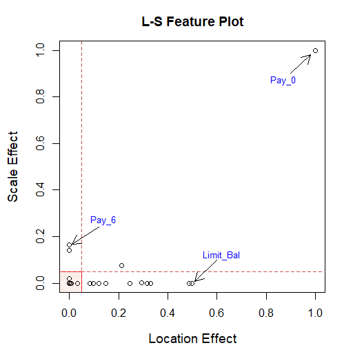
UCI Credit Card data. The dataset is available in the UCI Machine Learning Repository. It contains records of cardholders from an important Taiwan-based bank. For each customer, we have a response variable denoting: default payment status (Yes = 1, No = 0), along with predictor variables (e.g., gender, education, age, history of past payment, etc.). We randomly partition the data into training and test sets, with an 80-20 split, repeated times. We measure the prediction accuracy using AUC (the area under the ROC curve). Fig. 6 compares two kinds of lasso-logistic regressions: (i) usual version: based on feature matrix ; and (ii) LP-copula version: based on feature matrix . As we can see, LP-copula based additive logistic regression classifier significantly outperforms the classical logistic regression model. To gain further insight into the nature of impact of each variable, we plot the lasso-smoothed location and scale coefficients:
L-stands for location and S-stands for scale. The purpose of the LS-feature plot is to characterize ‘how’ each feature impacts the classification task. For example, consider the three variables pay0, limitbalance, and pay6, shown in the bottom panel Fig. 6. Each one of them contains unique discriminatory information: pay0 has location as well as scale information, hence it appeared at the top-right of the LS-plot; The variable limitbalance mainly shows location differences, whereas the variable pay6 shows contrasting scale in the two populations. In short, LS-plot explains ‘why and how’ each variable is important using a compact diagram, which is easy to interpret by researchers and practitioners.
4 Conclusion: Copula-based Statistical Learning
This paper makes the following contributions: (i) we introduce modern statistical theory and principles for maximum entropy copula density estimation that is self-adaptive for the mixed(X,Y)—described in Section 2. (ii) Our general copula-based formulation provides a unifying framework of data analysis from which one can systematically distill a number of fundamental statistical methods by revealing some completely unexpected connections between them. The importance of our theory in applied and theoretical statistics is highlighted in Section 3, taking examples from different sub-fields of statistics: Log-linear analysis of categorical data, logratio biplot, smoothing large sparse contingency tables, mutual information, smooth- statistic, feature selection, and copula-based logistic regression. We hope that this new perspective on copula modeling will offer more effective ways of developing united statistical algorithms for mixed-().
Dedication: Two Legends from Two Different Cultures
This paper is dedicated to the birth centenary of E. T. Jaynes (1922–1998), the originator of the maximum entropy principle.
I also like to dedicate this paper to the memory of Leo Goodman (1928–2020)—a transformative legend of categorical data analysis, who passed away on December 22, 2020, at the age of 92 due to COVID-19.
This paper is inspired in part by the author’s intention to demonstrate how these two modeling philosophies can be connected and united in some ways. This is achieved by employing a new nonparametric representation theory of generalized copula density.
References
- Agresti (2013) Agresti, A. (2013), Categorical data analysis (3rd ed.), John Wiley & Sons.
- Aitchison and Aitken (1976) Aitchison, J. and Aitken, C. G. (1976), “Multivariate binary discrimination by the kernel method,” Biometrika, 63, 413–420.
- Arbous and Kerrich (1951) Arbous, A. G. and Kerrich, J. (1951), “Accident statistics and the concept of accident-proneness,” Biometrics, 7, 340–432.
- Barron and Sheu (1991) Barron, A. R. and Sheu, C. (1991), “Approximation of density functions by sequences of exponential families.” Annals of Statistics, 19, 1347–1369.
- Benzecri (1991) Benzecri, J. P. (1991), “Comment on Leo Goodman’s “Models, and Graphical Displays in the Analysis of Cross-Classified Data”,” Journal of the American Statistical Association., 86, 1112–1115.
- Efron and Hastie (2016) Efron, B. and Hastie, T. (2016), Computer Age Statistical Inference, vol. 5, Cambridge University Press.
- Fienberg (1971) Fienberg, S. E. (1971), “Randomization and social affairs: the 1970 draft lottery,” Science, 171, 255–261.
- Fienberg and Rinaldo (2007) Fienberg, S. E. and Rinaldo, A. (2007), “Three centuries of categorical data analysis: Log-linear models and maximum likelihood estimation,” Journal of Statistical Planning and Inference, 137, 3430–3445.
- Friedman et al. (2010) Friedman, J., Hastie, T., and Tibshirani, R. (2010), “Regularization paths for generalized linear models via coordinate descent,” Journal of statistical software, 33, 1.
- Gao et al. (2017) Gao, W., Kannan, S., Oh, S., and Viswanath, P. (2017), “Estimating mutual information for discrete-continuous mixtures,” in Advances in neural information processing systems, pp. 5986–5997.
- Genest et al. (2013) Genest, C., Nešlehová, J., and Rémillard, B. (2013), “On the empirical multilinear copula process for count data,” Bernoulli, 20, in press.
- Gilula et al. (1988) Gilula, Z., Krieger, A. M., and Ritov, Y. (1988), “Ordinal association in contingency tables: some interpretive aspects,” Journal of the American Statistical Association, 83, 540–545.
- Goodman (1991) Goodman, L. A. (1991), “Measures, models, and graphical displays in the analysis of cross-classified data (with discussion),” Journal of the American Statistical association, 86, 1085–1111.
- Goodman (1996) — (1996), “A single general method for the analysis of cross-classified data: reconciliation and synthesis of some methods of Pearson, Yule, and Fisher, and also some methods of correspondence analysis and association analysis,” Journal of the American Statistical Association, 91, 408–428.
- Greenacre (2018) Greenacre, M. (2018), Compositional data analysis in practice, CRC Press.
- Hastie et al. (2015) Hastie, T., Tibshirani, R., and Wainwright, M. (2015), “Statistical learning with sparsity,” Monographs on statistics and applied probability, 143, 143.
- Hoeffding (1940) Hoeffding, W. (1940), “Massstabinvariante Korrelationstheorie,” Schriften des Mathematischen Seminars und des Instituts fr Angewandte Mathematik der Universitt Berlin, 5, 179–233.
- Jaynes (1957) Jaynes, E. T. (1957), “Information theory and statistical mechanics,” Physical review, 106, 620.
- Koehler (1986) Koehler, K. J. (1986), “Goodness-of-fit tests for log-linear models in sparse contingency tables,” Journal of the American Statistical Association, 81, 483–493.
- Kraskov et al. (2004) Kraskov, A., Stögbauer, H., and Grassberger, P. (2004), “Estimating mutual information,” Physical review E, 69, 066138.
- Moon et al. (1995) Moon, Y.-I., Rajagopalan, B., and Lall, U. (1995), “Estimation of mutual information using kernel density estimators,” Physical Review E, 52, 2318.
- Mukhopadhyay (2017) Mukhopadhyay, S. (2017), “Large-Scale Mode Identification and Data-Driven Sciences,” Electronic Journal of Statistics, 11, 215–240.
- Mukhopadhyay (2021) — (2021), “Density Sharpening: Principles and Applications to Discrete Data Analysis,” Technical Report, arXiv:2108.07372, 1–51.
- Mukhopadhyay (2022) — (2022), “Modelplasticity and Abductive Decision Making,” Technical Report, arXiv:2203.03040, 1–27.
- Mukhopadhyay and Parzen (2020) Mukhopadhyay, S. and Parzen, E. (2020), “Nonparametric Universal Copula Modeling,” Applied Stochastic Models in Business and Industry, special issue on “Data Science”, 36, 77–94.
- Mukhopadhyay et al. (2012) Mukhopadhyay, S., Parzen, E., and Lahiri, S. (2012), “From data to constraints,” Bayesian Inference And Maximum Entropy Methods In Science And Engineering: 31st International Workshop, Waterloo, Canada, 1443, 32–39.
- Parzen and Mukhopadhyay (2013) Parzen, E. and Mukhopadhyay, S. (2013), “United Statistical Algorithms, LP-Comoment, Copula Density, Nonparametric Modeling,” 59th ISI World Statistics Congress (WSC), Hong Kong, 4719–4724.
- Seok and Kang (2015) Seok, J. and Kang, Y. S. (2015), “Mutual information between discrete variables with many categories using recursive adaptive partitioning,” Scientific reports, 5, 1–10.
- Simonoff (1983) Simonoff, J. S. (1983), “A penalty function approach to smoothing large sparse contingency tables,” The Annals of Statistics, 208–218.
- Simonoff (1985) — (1985), “An improved goodness-of-fit statistic for sparse multinomials,” Journal of the American Statistical Association, 80, 671–677.
- Simonoff (1995) — (1995), “Smoothing categorical data,” Journal of Statistical Planning and Inference, 47, 41–69.
- Sklar (1959) Sklar, M. (1959), “Fonctions de répartition à n dimensions et leurs marges,” Publ. Inst. Statistique Univ. Paris, 8, 229–231.
- Yates (1934) Yates, F. (1934), “Contingency tables involving small numbers and the test,” Supplement to the Journal of the Royal Statistical Society, 1, 217–235.
- Zelterman (1987) Zelterman, D. (1987), “Goodness-of-fit tests for large sparse multinomial distributions,” Journal of the American Statistical Association, 82, 624–629.
- Zeng et al. (2018) Zeng, X., Xia, Y., and Tong, H. (2018), “Jackknife approach to the estimation of mutual information,” Proceedings of the National Academy of Sciences, 115, 9956–9961.
5 Supplementary Appendix
A.1 Nonparametric LP-Polynomials
Preliminaries. For a random variable with the associated probability distribution , define the mid-distribution function as where is probability mass function. The has mean and variance . Define first-order basis function by standardizing -transformed random variable:
| (6.1) |
where and . Construct the higher-order LP-polynomial bases99 9 Here the number of LP-basis functions is always less than , where denotes the set of all unique values of . by Gram-Schmidt orthonormalization of . We call these specially-designed polynomials of mid-distribution transforms as LP-basis, which by construction, satisfy the following orthonormality with respect to the measure :
| (6.2) |
where is the Kronecker delta. Two particular LP-family of polynomials are given below:
gLP-Polynomial Basis. Let , where is a known distribution. Following the above recipe, construct parametric gLP-basis for the given distribution . For , one can show that see Mukhopadhyay and Parzen 2020 for more details.
eLP-Polynomial Basis. In practice, we only have access to a random sample from an unknown distribution . To perform statistical data analysis, it thus becomes necessary to nonparametrically ‘learn’ an appropriate basis that is orthogonal with respect to the (discrete) empirical measure . To address that need, construct LP-basis with respect to the empirical measure .
LP-unit Basis. We will occasionally express the ’s in the quantile domain
| (6.3) |
We call these S-functions the unit LP-bases. The ‘S-form’ and the ‘T-form’ will be used interchangeably throughout the paper, depending on the context.
LP-product-bases and Copula Approximation. The LP-product-bases can be used to expand any square-integrable function of the form . In particular, the logarithm of Hoeffding’s dependence function (2.3) can be approximated by LP-Fourier series:
| (6.4) |
Represent (6.4) in the quantile domain by substituting and to get the copula density expression (2.9).
A.2 Two Cultures of Maximum Entropy Modeling
The form of the maximum-entropy exponential model directly depends on the form of the set of constraints, i.e., the sufficient statistics functions. The maxent distribution depends on the data only through the sample averages for these functions.
Parametric maxent modeling culture: The traditional practice of maxent density modeling assumes that the appropriate sufficient statistics functions are known or given beforehand, which, in turn, puts restrictions on the possible ‘shape’ of the probability distribution. This parametric maxent modeling culture was first established by Ludwig Boltzmann in 1877, and then later popularized by E. T. Jaynes in 1960s.
Nonparametric maxent modeling culture: It proceeds by identifying a small set of most important sufficient statistics functions from data (Mukhopadhyay et al. 2012). In the next step, we build the maxent probability distribution that agrees with these specially-designed relevant constraints. We have used LP-orthogonal polynomials to systematically and robustly design the constraining functions. See, Section A.3 for more discussion.
A.3 Connection With Vladimir Vapnik’s Statistical Invariants
Vladimir Vapnik (Vapnik and Izmailov 2020) calls the sufficient statistics functions as ‘predicates’ and the associated moment constraints as ‘statistical invariants.’ While describing his learning theory he acknowledged that
“The only remaining question in the complete statistical learning theory is how to choose a (small) set of predicates. The choice of predicate functions reflects the intellectual part of the learning problem.”
The question of how to systematically design and search for informative predicates was previously raised by Mukhopadhyay et al. 2012 in the context of learning maxent probability models from data; also see Section 2.2 of the main article where we discussed some concrete strategies to address this problem. However, it is important to note that Vapnik and Izmailov 2020 works entirely within the traditional least-square ( risk) setup, instead of maximum-entropy framework.

A.4 Empirical Power Study
The simulation study is constructed as follows:
| Copula | Method | Values of | ||||
|---|---|---|---|---|---|---|
| 5 | 20 | 40 | 50 | 100 | ||
| 0.058 | 0.760 | 0 | 0 | 0 | ||
| 0.062 | 0.044 | 0.059 | 0.041 | 0.060 | ||
| Gaussian | 0.950 | 0.970 | 0 | 0 | 0 | |
| 0.920 | 0.970 | 0.960 | 0.940 | 0.960 | ||
| Gumbel | 0.790 | 0.960 | 0 | 0 | 0 | |
| 0.758 | 0.930 | 0.910 | 0.940 | 0.90 | ||
| Clayton | 0.860 | 0.950 | 0 | 0 | 0 | |
| 0.840 | 0.910 | 0.950 | 0.930 | 0.940 | ||
Step 1. Constructing tables with different dependence structures. We simulate independent random samples from the following copula distributions:
- •
Independent copula: ;
- •
Gaussian copula with ;
- •
Gumbel copula with parameter .
- •
Clayton copula with parameter .
The shapes of the copulas are shown in Fig. 7. We convert each bivariate dataset into contingency table (having equally spaced bins) of counts , with , , and .
Step 2. Simulating tables under null. Generate (null) tables with given row marginal and column marginal using Patefield 1981’s (1981) algorithm. It is implemented in the R-function r2dtable.
Step 3. Power approximation. We used null tables to estimate the 95% rejection cutoffs at the significance level . The power is estimated based on independence tests for different sizes of contingency tables: . We have fixed to compute the smooth- statistic, following Eqs. (3.22) and (3.26).
Result. The type I error rates and power performances are reported in Table 3. The test shows some strange Type-I error rate pattern: for medium-large contingency tables ( case), it acts as an ultra-liberal test with Type I error (, in box) much higher than the nominal level; while, for large-sparse cases (with ) it behaves as an ultra-conservative test that yields Type I error rate much lower (almost zero) than the nominal level. On the other hand, -test maintains the type-I error rates close to the significance level , even for highly sparse scenarios. In terms of power, the test is only reliable for the case. The higher power for the table is just a consequence of large type-I error phenomena. Conclusion: the conventional Wilks’ is not a trustworthy test, even for moderately large tables, and should not be used blindly as a “default” method. The smoothed performs remarkably well under all of these different scenarios and emerges as the clear winner.
References
- Mukhopadhyay and Parzen (2020) Mukhopadhyay, S. and E. Parzen (2020). Nonparametric universal copula modeling. Applied Stochastic Models in Business and Industry, special issue on “Data Science” 36(1), 77–94.
- Mukhopadhyay et al. (2012) S. Mukhopadhyay, E. Parzen. and S. N. Lahiri (2012). From data to constraints. Bayesian Inference And Maximum Entropy Methods In Science And Engineering: 31st International Workshop, Waterloo, Canada, 1443, 32–39.
- Patefield (1981) Patefield, W. (1981). Algorithm AS 159: an efficient method of generating random RC tables with given row and column totals. Journal of the Royal Statistical Society. Series C (Applied Statistics) 30(1), 91–97.
- Vapnik and Izmailov (2020) Vapnik, V. and R. Izmailov (2020). Complete statistical theory of learning: learning using statistical invariants. In A. Gammerman, V. Vovk, Z. Luo, E. Smirnov, and G. Cherubin (Eds.), Proceedings of the 7th Symposium on Conformal and Probabilistic Prediction and Applications, Maastricht, The Netherlands, 128, 4–40.
A.5 Additional Figures and Tables


| Months | High | Med | Low |
|---|---|---|---|
| Jan | 9 | 12 | 10 |
| Feb | 7 | 12 | 10 |
| Mar | 5 | 10 | 16 |
| Apr | 8 | 8 | 14 |
| May | 9 | 7 | 15 |
| Jun | 11 | 7 | 12 |
| Jul | 12 | 7 | 12 |
| Aug | 13 | 7 | 11 |
| Sep | 10 | 15 | 5 |
| Oct | 9 | 15 | 7 |
| Nov | 12 | 12 | 6 |
| Dec | 17 | 10 | 4 |
| 0 | 1 | 2 | 3 | 4 | 5 | 6 | |
|---|---|---|---|---|---|---|---|
| 0 | 0.17 | 0.15 | 0.07 | 0.02 | 0.01 | 0.00 | 0.00 |
| 1 | 0.11 | 0.12 | 0.08 | 0.01 | 0.03 | 0.01 | 0.00 |
| 2 | 0.03 | 0.04 | 0.03 | 0.02 | 0.01 | 0.00 | 0.01 |
| 3 | 0.02 | 0.01 | 0.02 | 0.02 | 0.00 | 0.01 | 0.00 |
| 4 | 0.00 | 0.00 | 0.01 | 0.01 | 0.00 | 0.00 | 0.00 |
| 7 | 0.00 | 0.01 | 0.00 | 0.00 | 0.00 | 0.00 | 0.00 |
| 0 | 1 | 2 | 3 | 4 | 5 | 6 | |
|---|---|---|---|---|---|---|---|
| 0 | 0.19 | 0.13 | 0.06 | 0.02 | 0.01 | 0.00 | 0.00 |
| 1 | 0.09 | 0.10 | 0.07 | 0.03 | 0.01 | 0.01 | 0.00 |
| 2 | 0.03 | 0.05 | 0.04 | 0.02 | 0.01 | 0.00 | 0.00 |
| 3 | 0.01 | 0.02 | 0.02 | 0.01 | 0.01 | 0.00 | 0.00 |
| 4 | 0.00 | 0.01 | 0.01 | 0.00 | 0.00 | 0.00 | 0.00 |
| 7 | 0.00 | 0.00 | 0.00 | 0.00 | 0.00 | 0.00 | 0.00 |