False signals of chaos from quantum probes
Abstract
We demonstrate that two-time correlation functions, which are generalizations of out-of-time-ordered correlators (OTOCs), can show ‘false-flags’ of chaos by exhibiting behaviour predicted by random matrix theory even in a system with classically regular dynamics. In particular, we analyze a system of bosons trapped in a double-well potential and probed by a quantum dot which is coupled to the bosons dispersively. This is an integrable system (considered both as separate parts and in total). Despite the continuous time evolution generated by the actual Hamiltonian, we find that the -fold two-time correlation function for the probe describes an effective stroboscopic or Floquet dynamics whereby the bosons appear to be alternately driven by two different non-commuting Hamiltonians in a manner reminiscent of the Trotterized time evolution that occurs in digital quantum simulation. The classical limit of this effective dynamics can have a nonzero Lyapunov exponent, while the effective level statistics and return probability show traditional signatures of chaotic behaviour. In line with several other recent studies, this work highlights the fact that the behavior of OTOCs and their generalizations must be interpreted with some care.
I Introduction
Two-time correlation (TTC) functions are indispensable tools in the investigation of the dynamics of quantum many-body systems. For example, a TTC of the form enters Kubo’s formula for the linear response of the observable at time due to the time-dependent perturbation at earlier times by the drive chaiken_lubensky. The wide utility of linear response theory means that TTCs are therefore a vital ingredient in calculations in quantum many-particle kinetics ranging from absorption spectra, to reaction rates and diffusion constants. They are also useful in assessing ‘quantumness’ through their connection to Leggett-Garg inequalities leggett08; emary14.
In this paper we consider a general -fold TTC function bhattacharyya19; haehl19; halpern18; shenker14; roberts17 which for Hermitian operators we define as
| (1) |
where , and is the expectation value taken with respect to a pure or mixed state. The first order TTC function describes a perturbation by operator at time followed by a ‘probe’ by operator at time like in the Kubo formula. This function is related to quantities such as the quantum fidelity which has been successfully employed as a means of detecting and characterizing quantum phase transitions (QPTs) zanardi06; chen07; buonsante07; quan06; ning08. However, in general, the first order TTC fails to capture the spread of information across a system from an initial perturbation. Thus, in recent years the second order TTC function has gained popularity and is often referred to as the out-of-time-ordered correlation (OTOC) function.
In addition to being more sensitive to QPTs than first order TTCs heyl18; sun19; mumford20, OTOCs have been used to identify the ‘scrambling’ of information across a system’s degrees of freedom yao16; swingle16; bohrdt17. For this purpose it is useful to express the OTOC function as an overlap between two states, where and and is some general state. When the operators are chosen such that they initially commute, , then is unity at , and at later times it decays as correlations build up and these operators no longer commute. In complex systems it turns out that there is typically an exponential decay where is some constant and is the decay rate.
The exponential sensitivity of OTOCs to information scrambling has led to the exciting idea that OTOCs might be capable of quantifying many-body quantum chaos (or stated more carefully, dynamics which would be chaotic in the classical limit) roberts15; maldacena2016a; maldacena2016b; zhu16; kukuljan17; rozenbaum17; cotler18; kurchan18; chen18; mata18; jalabert18; hamazaki18; herrera18; rozenbaum19; carlos19. The defining feature of classical chaos is an exponential sensitivity to initial conditions, i.e. the exponential increase in separation over time of initially close points in phase space, and is quantified by Lyapunov exponents. This behaviour is considered to be a prerequisite for ergodicity and thermalization which destroys any memory of the initial state and it therefore seems natural enough from an information-theoretic perspective that chaos should be related to information scrambling. In fact, it has been demonstrated in a number of specific examples that the OTOC decay rate is directly related to the Lyapunov exponent in the classical limit of a chaotic quantum system; these cases include the kicked rotor hashimoto2017, stadium billiard rozenbaum19, Dicke model carlos19 and kicked Dicke model sinha2021.
However, recently it has been shown that having for an OTOC does not necessarily indicate that the system is chaotic, but instead can be caused by information scrambling from dynamics near an unstable fixed point pappalardi18; hummel19. The simplest example of such cases is the exponential separation of trajectories at short times in the inverted harmonic oscillator, which in single-particle quantum mechanics gives rise to at finite and infinite temperatures from the OTOC hashimoto20. Furthermore, OTOCs in integrable many-particle systems such as the Lipkin-Meshkov-Glick model and the Dicke model (in the latter’s integrable phase) cameo20; xu20 also exhibit positive near unstable points resulting from second-order QPTs.
In this paper we provide another example of how TTCs can exhibit false-flags of chaos by showing that for a regular (i.e. nonchaotic) system the operator in Eq. (1) can display Wigner Dyson-type spectral statistics described by random matrix theory (RMT). RMT was first used in the 1950s to understand the statistical properties of the spectra of complex nuclei wigner51 and reached maturity in the 1980s with the realization (as encapsulated by conjectures such as that due to Bohigas, Giannoni, and Schmit bohigas1983; bohigas84) that fluctuations in the distances between energy levels have universal properties in the semiclassical regime (far above the ground state) that distinguish chaotic from nonchaotic systems. In fact, it seems that apart from a few atypical exceptions the spectral statistics of physical systems fall into one of four classes determined by ensembles of random Hermitian matrices. For classically integrable systems the statistics of the corresponding quantum energy levels are Poissonian, whereas for classically chaotic systems the corresponding energy level fluctuations follow those of either the Gaussian orthogonal ensemble (GOE), the Gaussian unitary ensemble (GUE) or the Gaussian symplectic ensemble (GSE) independent of the details of the system and depending only on the symmetry properties of the Hamiltonian under canonical transformations. For a Floquet-type unitary operator [such as that effectively given by Eq. (1)], these ensembles are changed from Gaussian to circular ensembles (COE etc.) because the eigenvalues should have a magnitude of one.
The system we use to illustrate these features is a simple model consisting of identical bosons occupying two modes and coupled to a single qubit probe (atomic quantum dot) and has previously been discussed in a considerable number of theoretical proposals, e.g. bausmerth07; Rinck2011; mulansky11; gerritsma12; mumford14a; mumford14b; joger14; ebgha19; chen2021. In general this system is chaotic mumford14a; chen2021, but in this paper we do not allow the qubit to exchange energy with the bosons (dispersive limit of the interaction) and this renders the model integrable. Our model is relevant to experiments with bosonic Josephson junctions, e.g. Bose-Einstein condensates (BECs) in double well potentials albiez05; Levy07; LeBlanc2011; trenkwalder16, or spinor condensates with two internal states zibold10; Gerving12, if an additional impurity atom or ion zipkes10 is added. Alternatively, the same Hamiltonian (Ising model with long-range interactions) can be realized with trapped ions, again with two internal states Bohnet16, and again a distinguished ‘impurity’ atom or ion should be added to the system. Solid state Josephson junctions might offer another route to realize the type of dynamics we will discuss here Zhu2001; DeFranceschi2010; Pal2018.
The structure of the rest of this paper is as follows: Sec. II presents the details of the model (bosons+probe) to be used and Sec. III examines how a TTC of operators in the subspace belonging to the probe can be written as a periodic Floquet operator acting purely on the bosons. In Sec. IV the classical dynamics generated by this Floquet operator is examined, including the classical Lyapunov exponent which is a signature of chaos. Sec. V turns to quantum properties: Sec. V.1 examines the quasienergy level spacings of the Floquet operator and compares against the results of RMT, while Sec. V.2 treats the quantum TTC as a survival amplitude which leads naturally to computations of the inverse participation ratio and further comparisons against RMT. Conclusions are presented in Sec. VI. This paper also has three appendices where details of the calculations and some extra supporting results are given.
II Model
Our model couples the two-mode Bose-Hubbard model, which describes interacting bosons hopping between two sites, to a single two-state atomic quantum dot (AQD), i.e. a qubit. In order to put the qubit and the bosons on a similar footing it is convenient to express the boson operators in terms of collective spin operators
| (2) |
where . Using the Schwinger representation the same collective spin operators can alternatively be defined via annihilation and creation operators acting on the sites: If we label the two sites of the Bose-Hubbard model as (left) and (right) then the number difference between the left and right sites can be written , where () is the creation (annihilation) operator for a boson on the left/right site obeying the usual commutation relations where . Similarly, we have which takes a boson from one site and puts it onto the other (plus the reverse process to make the operator hermitian), thus producing mode coupling (tunneling).
In this way one finds that, up to constant terms, the total Hamiltonian can be written (for full details see mulansky11),
| (3) |
where , and are the boson, dot and boson-dot interaction Hamiltonians, respectively, and are given by
| (4) | |||||
| (5) | |||||
| (6) |
Here, the AQD operators are single Pauli matrices and are distinguished from the boson Pauli matrices by the absence of a superscript. The parameters in this Hamiltonian have the following definitions: is the boson-boson interaction energy, is the boson hopping/tunneling energy, is the energy imbalance between the two boson modes, is the energy imbalance between the two AQD modes and is the coupling energy between the AQD and the bosons.
It is important to note that there is no hopping term ( operator) in the dot’s Hamiltonian and so it cannot make transitions between its two states, i.e. , and this gives a dispersive interaction between the bosons and the AQD. The AQD therefore plays a somewhat passive role in the dynamics of the bosons: from we see that the effect of the AQD is to modify the tunneling energy of the bosons, either having no effect or suppressing it depending on whether the AQD is initialized in its excited or ground state, respectively. It has previously been shown that when the AQD is allowed to make transitions the classical dynamics displays chaos above a certain critical value of mumford14a, and without these transitions the dynamics is regular. Nevertheless, we will show in this paper that when AQD operators are used in Eq. (1), apparently chaotic dynamics emerge in the TTC due to the presence of the AQD.
One way to realize the Hamiltonian in Eq. (3) is with a BEC trapped in a double well potential in the two-mode regime and coupled to a distinguishable atom trapped between the two wells, see Fig. 1. This dot atom could be a different species to the rest of the atoms or simply be in a different hyperfine state. In fact the dot atom need not even be trapped between the two wells, and could instead be allowed to tunnel back and forth between the two wells like the bosons Rinck2011; mulansky11; chen2021. However, in order for the interaction to be dispersive in this case the energy difference between the symmetric and antisymmetric states of the dot atom should be much greater than all the other energies so that it remains in just one state during the dynamics.
For such an ultracold atom realization the parameters in Eqs. (4)-(6) can all be controlled using external fields: and contain the boson-boson and boson-dot s-wave scattering lengths, respectively, and can be controlled via the Feshbach resonance technique muessel15; perrin09; is the tunneling energy between the two BEC wells and can be controlled by raising or lowering the height of the barrier, e.g. by laser intensity; is the energy imbalance between the two wells and can be controlled by providing a tilt between them via external fields with spatial gradients; is the energy difference between the first two states of the AQD. An alternative realization, with slightly modified parameter definitions, makes use of internal states (for both the bosons and the AQD) rather than spatial states, although all the atoms should then be tightly trapped so that they occupy a single spatial mode. The tunneling between states in this case must be driven by laser or radio frequency radiation depending on whether the different internal states are different electronic orbitals or hyperfine states.

Yet another way to realize the boson-impurity model is via ions immersed in a BEC. In the experiment discussed in Ref. zipkes10 a single ion was trapped inside an BEC and the experiment demonstrated independent control of the ion and the BEC. Furthermore, temperatures where ion-atom collisions are dominated by the s-wave channel are being approached pinkas20. The Hamiltonian can also be realized using a linear ion trap system using with effective magnetic fields generated by stimulated Raman transitions hess17.
III Correlation function dynamics: Floquet operator
Our philosophy in this paper is to treat the AQD as a probe of the boson dynamics and hence the operators we shall use in Eq. (1) are all AQD operators. In fact, for simplicity we use for both operators and where, of course, we evolve as a function of time but keep at . Furthermore, we shall assume that at the probe and bosons are uncorrelated so that the initial state of the system is a product state of the form where is the state of the BEC and is the excited state of the quantum dot (starting the dot in the ground state works as well). This is, therefore, the state we use for evaluating the correlator . In addition, we make two simplifications to Eqs. (4)-(6): first, since the AQD Hamiltonian will only produce an overall dynamical phase in our calculations which will not affect the results, so we set , and second, without loss of generality we set (we shall explain this last condition below).
Under these conditions we find that the -fold TTC reduces to a correlation function evaluated purely within the bosonic state
| (7) |
where is a Floquet operator that repeatedly applies ( times) the unitary operator
| (8) |
The derivation of this result is given in Appendix A where it is shown that the two Hamiltonians appearing in are given by
| (9) | ||||
| (10) |
In line with the reduction of the full state to only the bosonic state in Eq. (7), it is notable that these effective Hamiltonians depend only on the boson operators and are different versions of given in Eq. (4). Hence, the general TTC has turned into a survival amplitude for the BEC part of the total state after applications of the operator . The different signs in front of the two Hamiltonians mean that the Floquet operator describes a system being shaken forwards and backwards (with slightly different forwards and backwards evolution) in time where the elapsed time is the length of each part of the shake and the order of the TTC is the number of cycles.
Our choice of simplifies the Hamiltonian so that does not appear, as explained in Appendix A. This tuning is not central to the validity of our results: other choices will simply add a finite hopping term to . However, the vanishing of the term in the other Hamiltonian is a robust feature of having an uncorrelated initial state. This is a special choice, but also a very reasonable one. As long as the initial state is separable, one will always get forward and backward pieces like in Eqns. (9) and (10).
We note in passing that a related issue to the one discussed in this paper is also an important consideration in digital quantum simulation, i.e. the breakup of continuous time evolution into separate steps. This sometimes goes under the name of Trotterization (after Trotter-Suzuki decompositions) and careful control of the errors induced by this process is critical to the accuracy of such simulations. In fact, it has been shown that there is a deep connection to chaos because chaotic systems are intrinsically less stable against such errors than nonchaotic ones sieberer19.



IV Classical correlation function dynamics
We begin our analysis of the correlation function dynamics by checking for classical chaos. The classical theory is given by the mean-field approximation and it is known that in this limit the two-mode Bose Hubbard model, which describes the bosonic part of the system, is equivalent to a non-rigid pendulum which is an integrable system Smerzi97. When coupled to an impurity spin the total system can be mapped in certain regimes onto a double pendulum mulansky11 which is in general chaotic, although in the present dispersive case the second pendulum has a constant angular momentum which keeps the model integrable.
The mean-field versions of our various Hamiltonians are derived in Appendix B. For example, it is shown that the mean-field version of the total Hamiltonian is given by Eq. (37) which is obtained by replacing the mode operators with complex numbers and taking the thermodynamic limit . From there, Hamilton’s equations of motion can be used to generate the dynamics. In the case of and (the mean-field limits of and , respectively), the dynamics are produced by using Hamilton’s equations of motion for for a period of time , then we switch to Hamilton’s equations for for the same period of time, and repeat this intertwining process for cycles.
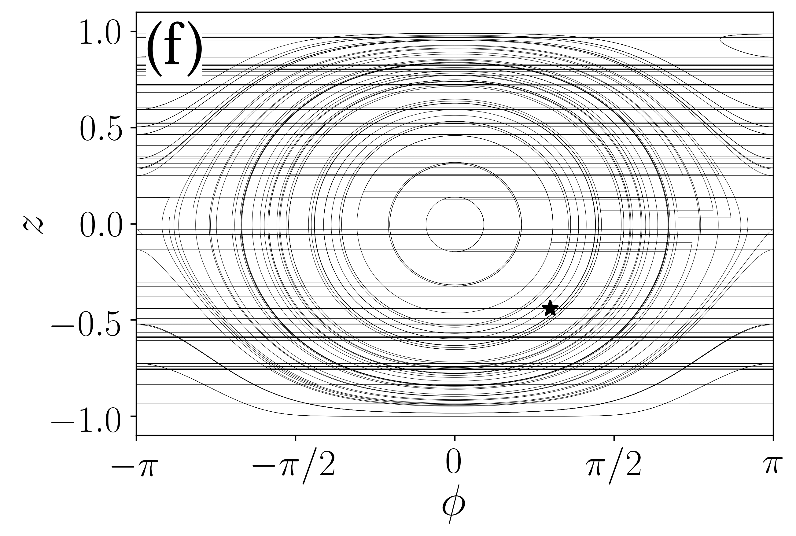
In Fig. 2 we plot the phase space dynamics of the BEC mean-field variables
| (11) |
which are the scaled number difference and phase difference between the left and right wells, respectively. Each row has a different initial condition represented by a black star. At short times (left column) the dynamics only accesses limited regions of phase space, especially if the system is initialized near the stable fixed point at . However, at longer times (right column) the dynamics becomes ergodic and independent of the initial conditions which is a hallmark of classical chaos. In fact, Fig. 2 shows how ergodicity is established despite the two parts of the time evolution being separately integrable: the trajectories conserve , so they travel only along the direction, essentially providing a pathway to different energy contours of , along which the orbit proceeds.
To quantify the chaotic dynamics we numerically compute the Lyapunov exponent and the results are plotted in Fig. 3 as a function of . Each data point is obtained from a phase space average taken with respect to many random initial states. When the trajectories are exponentially separating in time and hence we have chaos. As expected from Fig. 2, for relatively short periods () the trajectories tend to stay in a small subregion of phase space leading to . As the shake period is increased () the Lyapunov exponent becomes nonzero and the correlator dynamics becomes chaotic. For a comparison with the actual model see Fig. 6 in Appendix B where a plot of versus shows that , demonstrating that is regular. These results give us the first hint that the dynamics of the general TTC function can be chaotic even for a nonchaotic system.
V Quantum correlation function dynamics
We now turn to the fully quantum problem to look for evidence of so-called ‘quantum chaos’ in the correlator dynamics. To this end we first examine the spectral statistics of the Floquet operator and compare to RMT and second we calculate the survival probability.
V.1 Eigenphases and Spacings of the Floquet Operator
We first consider the Floquet operator in Eq. (8). Recently it was shown that in a quantum stadium billiard model (which has a classical limit which is chaotic) the spectral statistics of the operator , which contains an out-of-time-ordered commutator, align well with the predictions from RMT rozenbaum19. Similar results were found when analyzing the spectral statistics of a Floquet operator for a shaken system when its corresponding classical system is chaotic sieberer19. We will follow this route here and analyze the spectrum of . This is a unitary operator, but rather than work with its complex eigenvalues , we instead examine the statistical properties of its eigenphases .
First, we note that the eigenphases are time dependent in a nontrivial way which can be seen by writing in terms of a single effective Hamiltonian . Using the Baker-Campbell-Hausdorff formula,
| (12) |
we find that for our system can be written at short times as
| (13) |
At each moment in time the effective Hamiltonian yields a set of instantaneous eigenstates such that where is the set of instantaneous eigenenergies. From Eq. (13), we can see at early times the dynamics is simply due to , however, as increases more terms contribute to and the dynamics of the eigenenergies become complicated. Since , we expect the eigenphases to inherit this complicated behavior and this can indeed be seen in Fig. 4(a) where they are plotted as a function of time. At early times the magnitude of the eigenphases increases linearly until at around they begin to wind around the interval at which point tiny avoided crossings form (they are at first too small to see at the scale of the the figure, however when zoomed-in incredibly narrow avoided crossings become visible). At around the avoided crossings begin to widen and at late times the eigenphases are well separated and display the equivalent of level repulsion found in time-independent chaotic systems.


Rather than examine the full statistical distribution of the eigenphases, we instead calculate the average spacing ratio oganesyan07,
| (14) |
where is the difference between adjacent eigenphases and is the size of the BEC Hilbert space. The spacing ratio takes on distinct values depending on which RMT ensemble the eigenphases follow, if they follow any at all. For our case, having destroys the parity symmetry of the system leaving only time reversal symmetry. We therefore expect that should obey the circular orthogonal example (COE) result of . Fig. 4(b) shows clearly that does indeed oscillate around the COE result provided we consider longer times . In fact, comparing panels (a) and (b) in Fig. 4 we see that the dip in in the range corresponds to the range of times when the eigenphases first begin to wind around the full interval and form small avoided crossings. The time at which the dip occurs and how low it is are nonuniversal features that depend on the parameters of the system. For the avoided crossings of the eigenphases begin to widen and eventually show the chaotic result of level repulsion quantified by .
V.2 Survival Probability
Returning to Eq. (7), we focus our attention back on . More precisely, we study its squared absolute value which corresponds to the return probability . Furthermore, based on the results of the last section we expect the clearest evidence of chaos to come from the long time average of . We start by inserting the resolution of identity, (expressed in terms of the eigenvectors of ), into . This gives
| (15) | |||||
Here, and from now on, we suppress the subscript “B” on . Since the eigenstates and eigenenergies of are complicated functions of time, even the qualitative behaviour of the long time average of Eq. (15) is not immediately clear. For large enough TTC order , the phase factor will oscillate rapidly making all terms where approximately equal to zero (the “diagonal approximation”). This condition is satisfied naturally in the chaotic regime due to level repulsion of the eigenenergies. The level repulsion of the corresponding eigenphases is shown in Fig. 4, so we should expect the same for the eigenergies resulting in no degeneracies in the spectrum. Thus, when is large enough, the long time average of , , can be written as
| (16) | |||||
Thus, the survival probability becomes equal to the inverse participation ratio (IPR) of the state over the basis states of (or ) where the participation ratio (PR) is defined as
| (17) |
and is used to quantify how spread a state of interest is over a reference basis . What remains to be done is to explore the effect of different BEC states in which the correlation function is evaluated, and we shall see that this choice can affect the outcome of .
A generic state (e.g. one taken at random, absent any special symmetry), has complex coefficients in the basis of (i.e. the set of Fock states where the eigenvalues are half the boson number difference between the two sites) and is best modelled by CUE, whose states are uniformly distributed on the unit sphere in . If, however, we select a single eigenstate of the operator for our TTC, there is a shift instead to COE statistics due to the fact that these are eigenstates of , ultimately changing the symmetry of . This can be seen explicitly from the TTC, using Eq. (7),
| (18) |
where the phase can be neglected because we are interested in the survival probability . The evolution operator in Eq. (18) is related to the Floquet operator by
| (19) |
and has the additional symmetry , meaning its eigenstates have real components. Therefore, when considering the eigenstates as our basis, the time-dependent eigenstates of are not taken from matrices in the CUE (since those states have complex components) and instead are best modelled by random matrices in the COE, for which the states are distributed uniformly on the unit sphere in .


There exist signatures of chaos in both the survival probability of a single state, , and for ensembles of states. For the purposes of this article, we will focus on general features of the survival probability and so we will average over an entire basis, however a more in depth discussion of individual survival probabilities can be found in Appendix C. Performing the average over a basis , we can write the sum over individual as
| (20) |
where the bar over signals the average over the entire basis. If we use a random basis or the basis states of the operator sieberer19, we expect the average IPR to take on the CUE prediction,
| (21) |
where in the thermodynamic limit, , and hence . Meanwhile, if we use the basis of eigenstates, we expect the average IPR to take on the COE prediction,
| (22) |
for which as .
Following Schiulaz et al. schiulaz19, we can also calculate the Thouless time for a fully connected model like ours in the COE and CUE ensembles. describes the time at which the wavefunction first extends over the entire many-body Hilbert space, and is thus the time at which universal RMT predictions begin to govern the dynamics. For spatially extended systems, generally depends on the system size schiulaz19; sierant20, however for a fully connected model
| (23) | ||||
| (24) |
where these times are expressed in units of .
In Fig. 5(a) we plot numerical evaluations of averaged over the basis. Since at short times , the survival probability is briefly constant, and subsequently drops off to fluctuate near its relaxation value. The red dashed line is the long-time average and takes the value , an approximately error from its expected value of , shown as a solid cyan line. Although the survival probability has large amplitude oscillations, the long time average agrees well with the RMT prediction in Eq. (21). It is not required that we average over any particular basis in order to agree with the prediction in Eq. (21), only that the basis does not introduce any special symmetries to . As a demonstration, panel (b) shows the survival probability averaged over a randomly generated complex orthonormal basis (via a QR decomposition of a randomly populated complex matrix), which we denote . The long-time average in the random basis is , and agrees extremely well (within ) with . Finally, panel (c) of Fig. 5 shows averaged over the basis. The long-time average is , again shown as a red-dashed line, and has an approximately deviation from . In each image, the TTC order is and the system size is .
Taken together, the plots shown in Fig. 5 (see especially the log-log plots in the insets) indicate that the effective dynamics of the -fold TTC are regular at short times, then undergo a transition period until approximately , shown in all panels as a vertical dashed line according to Eqs. (23)-(22), after which the survival probability settles down, or at least oscillates about a universal value given by its RMT prediction in the respective ensemble. In general, we expect the agreement between the numerical result and the theoretical predictions given in Eqns. (21) and (22) to improve for higher TTC order and correspondingly longer time averages.
VI Summary and Conclusion
In this paper, we have given a proof-of-concept that conventional signals of chaotic behaviour, including level statistics, classical Lyapunov exponents, and RMT predictions can arise from generalized -fold TTCs even when starting from a non-chaotic Hamiltonian. This is significant because TTCs, and more specifically OTOCs (the case), are commonly used as diagnostic tools for what is often called quantum chaos. Higher-order TTCs have been the focus of some previous studies bhattacharyya19; haehl19; halpern18; shenker14; roberts17, including as an improvement of the standard four-point OTOC as a diagnostic of chaos, and so the emergence of signatures of chaos as a result of the form of the TTC is therefore of interest.
In our case we chose a rather simple system consisting of a bosonic Josephson junction coupled dispersively to an AQD or impurity spin. This has the benefit of being integrable and thus all the signals of chaos we find are genuinely in the TTC not the original dynamics. Importantly, both the parameters and must be nonzero in the system we are considering so that there are noncommuting pieces in the Hamiltonian. In particular, would allow the vanishing of the commutator , resulting in trivial dynamics, while is necessary to destroy the parity symmetry and thereby allow the eigenstates of and to be modelled by the appropriate ensembles in RMT. However, the simplicity of our system also means that even the effectively shaken -fold TTC is only weakly chaotic and thus our survival probabilities do not rapidly converge to the RMT values (for our parameters the deviation can be as large as ). However, we also saw evidence that the bases of and remain in some sense special (being the eigenstates of the two pieces of the Hamiltonian) whereas when a truly random basis was chosen we obtained excellent agreement with deviation of less than .
There remain signatures of chaos which we have not addressed here. For example, we have not attempted to identify a quantum Lyapunov exponent (one typically uses and finds that shen17, where is some constant). Rather, in Sec. IV we have merely looked directly at the classical Lyapunov exponent obtained from the mean-field equations of motion for the -fold TTC. Furthermore, for a chaotic system obeying the RMT predictions outlined in this paper, it is expected that there exists a ‘correlation hole’ (a signature of correlations in level statistics) in the survival probability with a minimum at pechukas84; leviandier86; alhassid92; schiulaz19; hererra19, which proceeds to ramp towards the saturation value. We have not identified a correlation hole in the TTCs studied here, likely because the transition from a regular to chaotic system occurs explicitly in time, so level correlations will not be detectable prior to .
Acknowledgements.
WK is grateful to Greg Kaplanek for useful discussions. We acknowledge the Natural Sciences and Engineering Research Council of Canada (NSERC) for funding.Appendix A TTC Calculation
We consider the two-time correlator,
| (25) |
where and assume that and initially commute. Selecting , that is, the hopping operator on the Hilbert space of the quantum dot,
| (26) | ||||
| (27) | ||||
where we have made use of the fact that for some function of the Pauli spin matrices , .
For the expectation value we assume a product state , where is a general state of the BEC and is the excited state of the AQD. The and factors in Eq. (27) act as projectors onto the excited and ground AQD states, respectively. In particular, the operator appearing in the right hand exponential acts as twice the identity operator on the ket and thus passes through this exponential replacing all the factors by the number 2. Meanwhile, the other exponential contains which annihilates and so expanding out the exponential in a Taylor series we find all the AQD operators vanish and we can re-sum the exponential with only the boson operators. As a result we find the surprising result that the correlation function becomes completely independent of the AQD and we are left with
| (28) | ||||
The term results in a global phase which we can choose to set to zero, and we are free to select as we wish; we choose to remove all terms in as described in the main text, so that we finally achieve,
| (29) | ||||
| (30) |
Appendix B Mean-Field Hamiltonian and Equations of Motion
In order to write down the mean-field approximation to the quantum Hamiltonians given in Eqns. (3), (9), and (10), we first write the spin operators in terms of their corresponding Schwinger representations,
| (31) | ||||
| (32) |
where annihilates (creates) a boson in the left/right well. The quantum dot operators can be similarly written, using ,
| (33) |
Next, we assume that in the classical limit , we can replace the boson operators by complex numbers . We can also make a similar replacement for the dot (the “mean-field” theory is in fact exact for the dot), and then defining , , , and we have the substitution rules,
| (34) | ||||
| (35) | ||||
| (36) |
Hence, the mean-field Hamiltonian () is,
| (37) |
where all energies on the RHS are measured in terms of . Hamilton’s equations give,
| (38) | ||||
| (39) | ||||
| (40) | ||||
| (41) |
Likewise, the mean-field approximations for and are,
| (42) | ||||
| (43) |
The classical trajectories for Eqs. (42)-(43) are similarly calculated using Hamilton’s equations, however the set of conjugate variables is no longer present,
| (44) | ||||
| (45) | ||||
| (46) | ||||
| (47) |
The dynamics are governed by repeatedly alternating between and for a time .

In Fig. 3 of the main text, we show the effects of tuning the time at which the TTC is measured on the Lyapunov exponent for the classical Hamiltonians (42)-(43). Alternatively, in Fig. 6, we demonstrate the presence of a positive classical Lyapunov exponent for the system alternating between and as a function of the bosonic interaction energy. The original Hamiltonian has no appreciable Lyapunov exponent while the shaken system rapidly develops exponential separation of trajectories after . The distance between trajectories and in the BEC coordinates corresponds to a great-circle distance on the Bloch sphere,
| (48) |
which can be used to calculate .
Appendix C Individual Survival Probability
In Sec. V.2 of the main text we concerned ourselves mainly with the general features of the survival probability without specifically selecting states. The qualitative nature of broadly follows (the average), although it is more sensitive due to the lack of averaging over initial states. The saturation values when not averaged over the bases are then,
| (49) | ||||
| (50) |


In Fig. 7, we show the survival probability for three different states using and at and . Panel (a) shows the survival probability for , which is the ground state of the operator and also a coherent state. Much like the average, the survival probability is roughly constant for short times, then drops off, saturating at approximately , which is within of the CUE value of . For panel (b), we chose an initial state which is Gaussian (but not a coherent state) in the basis,
| (51) |
This broader state has excellent agreement with the CUE value at approximately , within . Finally, in panel (c), we instead choose a member of the basis, . The return probability of this state demonstrates sharp peaks reminiscent of dynamical phase transitions (DPT) and subsequently saturates at , approximately higher than .
Comparing the actual saturation values with those predicted in Eqs. (49)-(50), we find that the relative errors can be fairly large, on the order of 10-15. However, the errors on individual states can be extremely sensitive to parameter shifts. For example, a change to (deeper into the ‘chaotic’ region, extrapolated from Fig. 6) can reduce the error from the coherent state () to approximately , that is error from the value.
The return probability can occasionally reach extremely small orders of magnitude, especially for larger , at which machine-precision exact diagonalization becomes insufficient to properly resolve . This effect occurs in the regular regions prior to in panel (c) of Fig. 7, where DPT-like sharp valleys can only be resolved with precision on the order of decimal places (increasing with ). The extreme sensitivity of numerical noise in the Loschmidt echo in similar systems has been identified in Ref. homrighausen17. The region which requires high sensitivity to properly resolve the dynamics is, however, not our primary concern since it is not the chaotic region.
References
- (1) P. M. Chaiken and T. C. Lubensky, Principles of Condensed Matter Physics (Cambridge University Press, New York, 1995).
- (2) A. J. Leggett, Realism and the Physical World, Rep. Prog. Phys. 71, 022001 (2008).
- (3) C. Emary, N. Lambert, and F. Noric, Leggett-Garg Inequalities, Rep. Prog. Phys. 77, 016001 (2014).
- (4) A. Bhattacharyya, W. Chemissany, S. Shajidul Haque, B. Yan, Towards the Web of Quantum Chaos Diagnostics, arXiv:1909.01894
- (5) F.M. Haehl, R. Loganayagam, P. Narayan and M. Rangamani, Classification of out-of-time-order correlators, SciPost Phys. 6 (2019) 001.
- (6) N. Y. Halpern, B. Swingle, and J. Dressel, Quasiprobability behind the out-of-time-ordered correlator, Phys. Rev. A 97, 042105 (2018).
- (7) S. H. Shenker and D. Stanford, Multiple shocks, J. High Energy Phys. 12, (2014) 046.
- (8) D. A. Roberts and B. Yoshida, Chaos and complexity by design, J. High Energy Phys. 04 (2017) 121.
- (9) P. Zanardi and N. Paunkovic, Ground state overlap and quantum phase transitions, Phys. Rev. E 74, 031123 (2006).
- (10) S. Chen, L. Wang, S. J. Gu, and Y. Wang, Fidelity and quantum phase transition for the Heisenberg chain with next-nearest-neighbor interaction, Phys. Rev. E 76, 061108 (2007).
- (11) P. Buonsante and A. Vezzani, Ground-State Fidelity and Bipartite Entanglement in the Bose-Hubbard Model, Phys. Rev. Lett. 98, 110601 (2007).
- (12) H. T. Quan, Z. Song, X. F. Liu, P. Zanardi, and C. P. Sun, Decay of Loschmidt Echo Enhanced by Quantum Criticality, Phys. Rev. Lett. 96, 140604 (2006).
- (13) W. Q. Ning, S. J. Gu, Y. G. Chen, C. Q. Wu, and H. Q. Lin, Concurrence and fidelity of a Bose–Fermi mixture in a one-dimensional optical lattice, J. Phys.: Condens. Matter 20, 235236 (2008).
- (14) M. Heyl, F. Pollman, and B. Dora, Detecting Equilibrium and Dynamical Quantum Phase Transitions in Ising Chains via Out-of-Time-Ordered Correlators, Phys. Rev. Lett. 121, 016801 (2018).
- (15) Z.-H. Sun, J.-Q. Cai, Q.-C. Tang, Y. Hu, and H. Fan, Out-of-Time-Order Correlators and Quantum Phase Transitions in the Rabi and Dicke Models, Ann. Phys. (Berlin) 532, 1900270 (2019).
- (16) J. Mumford, W. Kirkby, and D. H. J. O’Dell, Measuring out-of-time-ordered correlation functions with a single impurity qubit in a bosonic Josephson junction, J. Phys. B: At. Mol. Opt. Phys. 53 145301 (2020).
- (17) N. Y. Yao, F. Grusdt, B. Swingle, M. D. Lukin, D. M. Stamper-Kurn, J. E. Moore, and E. A. Demler, Interferometric Approach to Probing Fast Scrambling, arXiv:1607.01801 (2016).
- (18) B. Swingle, G. Bentsen, M. Schleier-Smith, and P. Hayden, Measuring the scrambling of quantum information, Phys. Rev. A 94, 040302(R) (2016).
- (19) A. Bohrdt, C. B. Mendl, M. Endres, and M. Knap, Scrambling and thermalization in a diffusive quantum many-body system, New J. Phys. 19, 063001 (2017).
- (20) D. A. Roberts and D. Stanford, Diagnosing Chaos Using Four-Point Functions in Two-Dimensional Conformal Field Theory, Phys. Rev. Lett. 115, 131603 (2015).
- (21) J. Maldacena and D. Stanford, “Remarks on the Sachdev-Ye-Kitaev model,” Phys. Rev. D 94, 106002 (2016).
- (22) J. Maldacena, S. H. Shenker, and D. Stanford, “A bound on chaos,” J. High Energy Phys. 2016, 106 (2016).
- (23) G. Zhu, M. Hafezi, and T. Grover, Measurement of many-body chaos using a quantum clock, Phys. Rev. A 94, 062329 (2016).
- (24) I. Kukuljan, S. Grozdanov, and T. Prosen, Weak quantum chaos, Phys. Rev. B 96, 060301 (2017).
- (25) E. B. Rozenbaum, S. Ganeshan, and V. Galitski, Lyapunov Exponent and Out-of-Time-Ordered Correlator’s Growth Rate in a Chaotic System, Phys. Rev. Lett. 118, 086801 (2017).
- (26) J. S. Cotler, D. Ding, G. R. Penington, Out-of-time-order operators and the butterfly effect, Ann. Phys. 396, 318-333 (2018).
- (27) E. B. Rozenbaum, S. Ganeshan, and V. Galistski, Universal level statistics of the out-of-time-ordered operator, Phys. Rev. B 100, 035112 (2019).
- (28) J. Kurchan, Quantum Bound to Chaos and the Semiclassical Limit, J. Stat. Phys. 171, 965 (2018).
- (29) X. Chen and T. Zhou, Operator scrambling and quantum chaos, arXiv:1804.08655 (2018).
- (30) I. G.-Mata, M. Saraceno, R. A. Jalabert, A. J. Roncaglia, and D. A. Wisniacki, Chaos Signatures in the Short and Long Time Behavior of the Out-of-Time Ordered Correlator, Phys. Rev. Lett. 121, 210601 (2018).
- (31) R. A. Jalabert, I. García-Mata, and D. A. Wisniacki, Semiclassical theory of out-of-time-order correlators for low-dimensional classically chaotic systems, Phys. Rev. E 98, 062218 (2018).
- (32) R. Hamazaki, K. Fujimoto, and M. Ueda, Operator Noncommutativity and Irreversibility in Quantum Chaos, arXiv:1807.02360 (2018).
- (33) E. J. Torres-Herrera, A. M. García-García, and L. F. Santos, Generic dynamical features of quenched interacting quantum systems: Survival probability, density imbalance, and out-of-time-ordered correlator, Phys. Rev. B 97, 060303 (2018).
- (34) J. Chávez-Carlos, B. López-del-Carpio, M. A. Bastarrachea-Magnani, P. Stránský, S. Lerma-Hernández, L. F. Santos, and J. G. Hirsch, Quantum and Classical Lyapunov Exponents in Atom-Field Interaction Systems, Phys. Rev. Lett. 122, 024101 (2019).
- (35) K. Hashimoto, K. Murata, and R. Yoshii, Out-of- time-order correlators in quantum mechanics, J. High Energy Phys. 2017, 138 (2017).
- (36) Sundip Sinha, Sayak Ray, and Subhasis Sinha, Fingerprint of chaos and quantum scars in kicked Dicke model: An out-of-time-order correlator study, J. Phys.: Condens. Matter 33 174005 (2021).
- (37) S. Pappalardi, A. Russomanno, B. Žunkovic, F. Iemini, A. Silva, and R. Fazio, Scrambling and entanglement spreading in long-range spin chains, Phys. Rev. B. 98, 134303 (2018).
- (38) Q. Hummel, B. Geiger, J. D. Urbina, and K. Richter, Reversible Quantum Information Spreading in Many-Body Systems near Criticality, Phys. Rev. Lett. 123, 160401 (2019).
- (39) K. Hashimoto, K.-B. Huh, K.-Y. Kim, and R. Watanabe, Exponential growth of out-of-time-order correlator without chaos: inverted harmonic oscillator, J. High Energy Phys. 2020, 68 (2020).
- (40) S. Pilatowsky-Cameo, J. Chávez-Carlos, M. A. Bastarrachea-Magnani, P. Stránský, S. Lerma-Hernández, L. F. Santos, and J. G. Hirsch, Positive quantum Lyapunov exponents in experimental systems with a regular classical limit, Phys. Rev. E 101, 010202(R) (2020).
- (41) T. Xu, T. Scaffidi, and X. Cao, Does Scrambling Equal Chaos?, Phys. Rev. Lett. 124, 140602 (2020).
- (42) E. P. Wigner, On the Statistical Distribution of the Widths and Spacings of Nuclear Resonance Levels, Proc. Cambridge Philos. Soc. 47, 790 (1951).
- (43) O. Bohigas, R.U. Haq, and A. Pandey, Fluctuation Properties of Nuclear Energy Levels and Widths: Comparison of Theory with Experiment. Nuclear Data for Science and Technology, (Reidel, Dordrecht, Netherlands, 1983).
- (44) O. Bohigas, M. J. Giannoni, and C. Schmit, Characterization of Chaotic Quantum Spectra and Universality of Level Fluctuation Laws, Phys. Rev. Lett. 52, 1 (1984).
- (45) I. Bausmerth, U. R. Fisher, and A. Posazhennikova, Quantum top inside a Bose-Einstein-condensate Josephson junction, Phys. Rev. A 75, 053605 (2007).
- (46) M. Rinck and C. Bruder, Effects of a single fermion in a Bose Josephson junction, Phys. Rev. A 83, 023608 (2011).
- (47) F. Mulansky, J. Mumford, and D. H. J. O’Dell, Impurity in a Bose-Einstein condensate in a double well, Phys. Rev. A 84, 063602 (2011).
- (48) R. Gerritsma, A. Negretti, H. Doerk, Z. Idziaszek, T. Calarco, and F. Schmidt-Kaler, Bosonic Josephson Junction Controlled by a Single Trapped Ion, Phys. Rev. Lett. 109, 080402 (2012).
- (49) J. Mumford, J. Larson, and D. H. J. O’Dell, Impurity in a bosonic Josephson junction: Swallowtail loops, chaos, self-trapping, and Dicke model, Phys. Rev. A 89, 023620 (2014).
- (50) J. Mumford and D. H. J. O’Dell, Critical exponents for an impurity in a bosonic Josephson junction: Position measurement as a phase transition, Phys. Rev. A 90, 063617 (2014).
- (51) J. Joger, A. Negretti, and R. Gerritsma, Quantum dynamics of an atomic double-well system interacting with a trapped ion, Phys. Rev. A 89, 063621 (2014).
- (52) M. R. Ebgha, S. Saeidian, P. Schmelcher, and A. Negretti, Compound atom-ion Josephson junction: Effects of finite temperature and ion motion, Phys. Rev. A 100, 033616 (2019).
- (53) J. Chen, K. Keiler, G. Xianlong, and P. Schmelcher, Impurity induced quantum chaos for an ultracold bosonic ensemble in a double-well, arXiv:2101.11209
- (54) M. Albiez, R. Gati, J. Fölling, S. Hunsmann, M. Cristiani, and M. K. Oberthaler, Direct observation of tunneling and nonlinear self-trapping in a single bosonic Josephson junction, Phys. Rev. Lett. 95, 010402 (2005).
- (55) S. Levy, E. Lahoud, I. Shomroni, and J. Steinhauer, The a.c. and d.c. Josephson effects in a Bose-Einstein condensate, Nature 449, 579 (2007).
- (56) L. J. LeBlanc, A. Bardon, J. McKeever, M. Extavour, D. Jervis, J. Thywissen, F. Piazza, and A. Smerzi, Dynamics of a Tunable Superfluid Junction, Phys. Rev. Lett. 106, 025302 (2011).
- (57) A. Trenkwalder, G. Spagnolli, G. Semeghini, S. Coop, M. Landini, P. Castilho, L. Pezzè, G. Modugno, M. Inguscio, A. Smerzi, and M. Fattori, Quantum phase transitions with parity-symmetry breaking and hysteresis, Nat. Phys. 12, 826 (2016).
- (58) T. Zibold, E. Nicklas, C. Gross, and M. K. Oberthaler, Classicial bifurcation at the Transition from Rabi to Josephson dynamics, Phys. Rev. Lett. 105, 204101 (2010).
- (59) C.S. Gerving, T. M. Hoang, B.J. Land, M. Anquez, C.D. Hamley, and M.S. Chapman, Non-equilibrium dynamics of an unstable quantum pendulum explored in a spin-1 Bose-Einstein condensate, Nat. Commun. 3 1169 (2012).
- (60) C. Zipkes, S. Palzer, C. Sias, and M. Köhl, A trapped single ion inside a Bose-Einstein condensate, Nature 464, 388 (2010).
- (61) J. G. Bohnet, B. C. Sawyer, J. W. Britton, M. L. Wall, A. M. Rey, M. Foss-Feig, and J. J. Bollinger, Quantum spin dynamics and entanglement generation with hundreds of trapped ions, Science 352, 1297 (2016).
- (62) Y. Zhu, Q. Sun, and T. Lin, Andreev bound states and the -junction transition in a superconductor/quantum-dot/superconductor system. J. Phys.: Condens. Matter 13, 8783 (2001).
- (63) S. De Franceschi, L. Kouwenhoven, C. Schönenberger and W. Wernsdorfer, Hybrid superconductor–quantum dot devices, Nature Nanotechnology 5, 703 (2010).
- (64) S. Pal and C. Benjamin, Tuning the 0– Josephson junction with a magnetic impurity: Role of tunnel contacts, exchange coupling, e–e interactions and high-spin states, Sci. Reports 8, 5208 (2018).
- (65) W. Muessel, H. Strobel, D. Linnemann, T. Zibold, B. Juliá-Díaz, and M. K. Oberthaler, Twist-and-turn spin squeezing in Bose-Einstein condensates, Phys. Rev. A 92, 023603 (2015).
- (66) H. Perrin, Ultra cold atoms and Bose-Einstein condensation for quantum metrology, EPJ-Special Topics 172, 37 (2009).
- (67) M. Pinkas, Z. Meir, T. Sikorsky, R. Ben-Shlomi, N. Akerman and R. Ozeri, Effect of ion-trap parameters on energy distributions of ultra-cold atom–ion mixtures, New J. Phys. 22, 013047 (2020).
- (68) P. W. Hess, P. Becker, H. B. Kaplan, A. Kyprianidis, A. C. Lee, B. Neyenhuis, G. Pagano, P. Richerme, C. Senko, J. Smith, W. L. Tan, J. Zhang, and C. Monroe, Nonthermalization in trapped atomic ion spin chains, Phil. Trans. R. Soc. A 375, 20170107 (2017).
- (69) A. Smerzi, S. Fantoni, S. Giovanazzi, and S. R. Shenoy, Quantum Coherent Atomic Tunneling between Two Trapped Bose-Einstein Condensates, Phys. Rev. Lett. 79, 4950 (1997).
- (70) F. Haake, Quantum Signatures of Chaos, vol. 54 of Springer Series in Synergetics (Springer, Berlin, Germany, 2010).
- (71) L. M. Sieberer, T. Alsacher, A. Elben et al. Digital quantum simulation, Trotter errors, and quantum chaos of the kicked top. npj Quantum Inf 5, 78 (2019).
- (72) V. Oganesyan and D. A. Huse, Localization of interacting fermions at high temperature, Phys. Rev. B 75, 155111 (2007).
- (73) M. Schiulaz, E. Jonathan Torres-Herrera, and Lea F. Santos, Thouless and relaxation time scales in many-body quantum systems, Phys. Rev. B 99, 174313 (2019).
- (74) P. Sierant, D. Delande, and J. Zakrzewski, Thouless Time Analysis of Anderson and Many-Body Localization Transitions, Phys. Rev. Lett. 124, 186601 (2020).
- (75) I. Homrighausen, N. O. Abeling, V. Zauner-Stauber, and Jad C. Halimeh, Anomalous dynamical phase in quantum spin chains with long-range interactions, Phys. Rev. B 96, 104436 (2017).
- (76) H. Shen, P. Zhang, R. Fan, and H. Zhai, Out-of-time-order correlation at a quantum phase transition, Phys. Rev. B 96, 054503 (2017).
- (77) P. Pechukas, Remarks on “quantum chaos”, J. Phys. Chem. 88, 4823 (1984).
- (78) L. Leviandier, M. Lombardi, R. Jost, and J. P. Pique, Fourier Transform: A Tool to Measure Statistical Level Properties in Very Complex Spectra, Phys. Rev. Lett. 56, 2449 (1986).
- (79) Y. Alhassid and R. D. Levine, Spectral autocorrelation function in the statistical theory of energy levels, Phys. Rev. A 46, 4650 (1992).
- (80) E. J. T.-Herrera and L. F. Santos, Signatures of chaos and thermalization in the dynamics of many-body quantum systems, Eur. Phys. J. Special Topics 227, 1897 (2019).