Observer Design for Nonlinear Systems with Equivariance

The celebrated scientist Stanislaw Ulam once stated that “studying nonlinear systems is like […] studying non-elephant animals” [Cam87]. There is such a vast array of behaviours and structures encapsulated in the term nonlinear that any analysis can only apply to a subclass of possible systems. Real world observer problems, even when highly non-linear, often have structure that can be exploited in the design of algorithms. For mechatronic and navigation systems one of the most common structures is symmetry. The present paper concerns how to exploit such symmetry to design high performance observers for nonlinear control systems.

Formally, symmetry is a property of the defining equations of motion of a system. A system is said to by symmetric if there is a transformation of the state-space (the symmetry) for which the equations of motion of the system are unchanged (an invariance) or change in a structured manner (an equivariance). For example, consider directional kinematics on a sphere

where the state $\eta\in\mathrm{S}^{2}$ is a direction on a sphere, $\Omega\in\mathbb{R}^{3}$ is an input, and $\times$ is the usual vector cross product. For an observer problem, measurements of the inputs $\Omega$ are provided by a velocity sensor such as an inertial measurement unit with rate gyroscopes providing velocity measurements in the body-fixed frame [MHT20]. The goal will be to estimate the direction $\eta$ from (noisy) velocity measurements and some additional (noisy) direction measurements. The directional kinematics (1) are equivariant under multiplication $\eta\mapsto Q^{\top}\eta$ by a (constant) rotation matrix $Q\in\mathbf{SO}(3)$. That is

The transformed kinematics are written in terms of a transformed state variable $\eta^{\prime}:=Q^{\top}\eta$ and a transformed input variable $\Omega^{\prime}:=(Q^{\top}\Omega)$. The symmetry of the equations of motion is expressed in the sense that the new kinematics $\dot{\eta}^{\prime}=-\Omega^{\prime}\times\eta^{\prime}$ are identical to the original equations. The input transformation $\Omega^{\prime}=Q^{\top}\Omega$ is important, it encodes the equivariance of the system. Invariant systems are a subclass of equivariant systems for which the input transformation is trivial, that is the transformed and original system use the same input. Invariance is particularly relevant for autonomous dynamical systems (with no inputs) and is a foundation principle of classical and modern mechanics. The presence of inputs leads naturally to equivariance playing an analogous role for nonlinear control systems.

In this paper, we consider nonlinear control systems with symmetry and propose an approach for the design of nonlinear observers that is based on two simple precepts:

• •

  Exploit the symmetry of a system.

• •

  Respect the geometry of a system.

The first precept leads to a foundation principle of equivariant observer design: that the observer state is formulated on the symmetry group rather than the state-space. For example, in the direction estimation problem discussed earlier, the symmetries are the set of all rotations in the special orthogonal group $\mathbf{SO}(3)$. The equivariant design approach poses the observer state $\hat{Q}\in\mathbf{SO}(3)$ as a rotation matrix while the estimate of the state is recovered by applying the symmetry $\hat{\eta}:=\hat{Q}^{\top}\mathring{\eta}$ to an arbitrary constant origin direction $\mathring{\eta}\in\mathrm{S}^{2}$. Note that the observer-state lies in a completely different, and higher dimensional, manifold $\hat{Q}\in\mathbf{SO}(3)$ compared to the system-state $\eta\in\mathrm{S}^{2}$, a general characteristic of equivariant observer design. This simple reparametrization is more powerful than it may appear at first glance. Whereas $\hat{\eta}$ is just a point on the sphere, the equivariant observer state $\hat{Q}$ corresponds to a symmetry diffeomorphism of the whole space $\hat{Q}^{\top}:\mathrm{S}^{2}\to\mathrm{S}^{2}$. Applying (the inverse of) this symmetry to the true state defines the equivariant error $e=\hat{Q}\eta\in\mathrm{S}^{2}$; a globally defined intrinsic error for the observer design problem. This construction should be compared to a classical observer design on a manifold where the observer/state error depends on local or embedded coordinates and is neither global nor intrinsic. The goal of equivariant observer design is to find dynamics on the symmetry group (the set of rotations $\mathbf{SO}(3)$ in this case) such that the observer state (the rotation $\hat{Q}$ in this case) evolves to force the error $e\to\mathring{\eta}$ to converge to the known fixed origin, leading to the state estimate $\hat{\eta}\to\eta$ to converge to the true-state.

Posing the observer-state as an element of the symmetry group raises the question of how to define observer dynamics, since the obvious copy of the state dynamics as an internal model is no longer an option. Recent work [MHT20] showed that (for an equivariant system) there is always an equivariant lift $\Lambda$ of the system dynamics. The lift function defines a set of dynamics on the symmetry group that project down to the true system dynamics on the state-manifold and provide the structure of an internal model for the observer architecture. For the simple example we are discussing¹¹ 1 Here $\Omega^{\times}$ denotes the $3\times 3$ skew-symmetric matrix that encodes the vector cross product $\Omega^{\times}\eta=\Omega\times\eta$. $\Lambda=\Omega^{\times}$ and the observer is

where the observer depends on an additional correction term $\Delta_{t}\in\mathfrak{so}(3)$, a skew-symmetric matrix in the Lie-algebra of $\mathbf{SO}(3)$ that is used to steer $e\to\mathring{\eta}$. For $\Delta_{t}\equiv 0$ the solutions of these observer-dynamics project $\hat{\eta}(t)=\hat{Q}(t)^{\top}\mathring{\eta}$ to solutions of the system, encoding the internal model principle fundamental in observer design despite the difference in observer-state and system-state spaces.

It remains to “design” the correction term $\Delta_{t}$. Here the equivariant properties of the lift $\Lambda$ play a key role in ensuring that the error dynamics are both globally defined and locally well conditioned. Indeed, for the simple direction estimation example

Although, the velocity dependent part of the error dynamics for a general system do not cancel, they can always be written as a globally defined function of the equivariant error $e$ and a known origin input. This structure in the error dynamics provides a foundation for a whole range of global nonlinear observer design methodologies [HZT+11, VCSO10, MHV11, HMT+11, THML12, GFJS12, BSO12, IS14, HHMT15, AMB16, HMH16, BAT17, LBHMS17, HHMT15, ZF18, WT19, HTH+19, HTH+20] as well as opening the door for principled observer design based on linearisation [BMR06, MS07, MS08, BMR08, BMR09, BMS09, ZTM13, BMGB13, BMAG15, BB15, STMA16, BB17, BB18, LAF19, PC20, vHM20, vGHM20].

In the present paper, we provide a principled analysis of a linearising observer design by adapting the extended Kalman filter to equivariant error coordinates [vHM20, vGHM20]. Here we draw on the second precept to respect the geometry. Only a single set of local coordinates, centred on the origin in error coordinates, is required in contrast to a classical EKF that depends on linearisations taken along a time-varying trajectories, and this leads to improved filter performance. Moreover, as shown in the seminal work of Barrau and Bonnabel [BB17], there is a canonical choice of local coordinates (the normal coordinates) for which the linearisation error is minimized, leading to improved filter performance. Finally, a careful application of the principles of extended Kalman filtering in error coordinates, taking account of the geometry of the space, leads naturally to a curvature modification of the Riccati equation corresponding to a parallel transport of the covariance estimate. We show that including this term in the Ricatti also improves the filter response, particularly during the transient phase. The resulting filter is termed the Equivariant Filter (EqF) (see also [vHM20, vGHM20]) and the design approach provides high performance filters for a wide range of equivariant nonlinear systems. Even for the simple direction estimation example discussed above, for which a classical EKF using stereographic coordinates is highly effective, the performance gain in following principled equivariant observer design is clearly shown in Figure 1 (see Section 7 for details of the simulation).

Symmetry in mechatronic systems is a natural consequence of the invariance of the physical laws that govern their dynamics. The field of geometric control systems [BL05, Jur97] is founded on this perspective and was highly active from the seventies through to the nineties with work still ongoing. Although early work in this field [van81, GM85, Nv85] considered symmetry for general control system models, the field matured towards using the Euler-Lagrange and Hamiltonian frameworks and exploiting symmetry for structural analysis of these dynamics [BL05, Jur97]. Despite some effort [AR03, MBD04, Bon10] this body of theory has not translated easily into observer and filter design. In contrast, working with simpler kinematic models has had significant impact in navigation systems [BB18]. An early contribution in this direction was the work of Salucedean [Sal91] on attitude estimation of a satellite. The original theory was extended a decade later [VF01, TS03] to incorporate bias estimation in the sensor measurements. This work was done in parallel with the established Multiplicative Extended Kalman Filter (MEKF) attitude estimators that had been first developed in the eighties [LMS82] but were still under active research at the turn of the century [Mar03, CBO06, CMC07]. It was around 2005 that the importance of robust attitude filtering for the growing Unmanned Aerial Vehicle (UAV) industry became clear and the resulting interest lead to a burst of activity [MHP05, BR05, HM06, BMR06, MS07] leading to the seminal papers [MHP08, BMR09] proposing simple, robust observers that were an enabling technology in the development of commercial systems. Although the quality of Inertial Measurements Units (IMUs) has now improved, these early attitude observers were key in overcoming the very high noise levels and unreliability of the IMUs available to the early UAV systems. There was a significant body of work done in the 2010s that extended and developed these ideas for attitude estimation [MHV11, THML12, GFJS12, BSO12, IS14, BAT17]. Analogous approaches have considered the Special Euclidean group $\mathbf{SE}(3)$ for pose estimation [VCSO10, HZT+11, HHMT15, WT19, LBHMS17], the Special Linear group $\mathbf{SL}(3)$ for homography estimation [HMT+11, HHMT15, HTH+19, HTH+20], and a number of works on velocity aided attitude estimation [BMR06, MS08, AMB16, HMH16]. A key contribution here was in the work of Bonnabel et al. [BMR08, BMS09] who introduced a new group structure, later denoted by $\mathbf{SE}_{m}(n)$ [BB16], that allowed second order translation kinematics to be modelled in the same group structure as first order kinematics in attitude. This group structure was also exploited to model the Simultaneous Localisation and Mapping problem [BB16, ZWS+17, MH17, MHT21]. In parallel Zlotnik et al. used a direct product structure [ZF18] for the SLAM problem.

There are several works over the last fifteen years that have developed general theory for classes of systems [BMR09, MTH13, BMAG15, BB17, MHT20, NvHM20]. Bonnabel and coauthors have built a theory for the Invariant Extended Kalman Filter (IEKF) in a series of papers [Bon07a, BMS09, BB15]. Although similar in spirit to the multiplicative extended Kalman filter [LMS82, CMC07] and the error state Kalman filter [RSB99, Sol17], the IEKF provides a clear design methodology for general systems posed on Lie-groups. This perspective has provided significantly more insight into the structural properties of observer systems on Lie-groups and lead to the definition of the “group affine” property [BB16, BB17, MT21] for which it is possible to prove powerful stability results for highly nonlinear systems. Stability and robustness of high performance filters can also be guaranteed by the direct design of Ricatti observers [HS18, WBT21]. An advantage of this approach is that the filters are not tied to a fixed linearisation structure, however, there is no standardised design methodology and each example must be considered independently. The majority of approaches in the literature, including IEKF, MEKF, and the Riccati observers, are only applicable to systems posed directly on a Lie-group. Equivariant systems on smooth homogeneous spaces, that is, systems on manifolds that support a smooth group action from a higher dimensional Lie-group [MTH13], is a more general class of systems to which analogous observer design principles can be applied. This perspective goes back to the origins of modern equivariant observer theory where direction estimation on $\mathrm{S}^{2}$, an homogeneous space under rotation action by $\mathbf{SO}(3)$, was proposed in [MPHS05] and lifted to $\mathbf{SO}(3)$ [MHP08] to obtain the complementary filter for attitude discussed earlier. A similar perspective also led from [Bon07b] to [BMR09] and recent work on Ricatti observers for direction estimation [HA18]. Unfortunately, direction kinematics was the only known example of a robotics application involving a true homogeneous system structure until the SLAM problem was considered over ten years later [MH17, MHT21]. The gauge invariance inherent in the SLAM problem induces a homogeneous space structure that underlies recent work by the authors [vHM20, vMHT20, vMHT19, vM21]. This perspective is critically important for the visual SLAM problem where cameras are the primary exteroceptive sensor and the SLAM problem can no longer be modelled [vGHM20] using the $\mathbf{SE}_{n+1}(3)$ geometry introduced by Barrau et al. [BB16]. In other recent work, Joshi et al. has also considered more general bundle structures for the equivariant observer problem [JMB20], Izadi et al. has exploited variational approaches [IS14], Lavoie considered $H_{\infty}$ observers [LAF19], Bourmaud et al. [BMGB13, BMAG15] proposed extended Kalman and unscented filters on Lie groups from first principles, Ng et al. introduced a semi-direct group structure [NvMH19, NvHM20] for second order kinematics, while Phogat et al. considered a direct product structure for general second order systems on Matrix Lie groups [PC20].

In order to improve filter performance above the second order optimality in local coordinates provided by the extended Kalman filter, Bonnabel and coauthors have proposed the invariant unscented Kalman filter [BBC17, BBB18, BBB20] that exploits the invariant structure of the problem to transport the sample points of the unscented filter. A similar algorithm was proposed in Bourmaud et al. [BMAG15]. This approach can be generalised to any parallelizable manifold [BBB20] and corresponds to placing a flat geometric structure on the space. Using a flat geometry goes counter to other recent work Loianno et al. [LWK16] in applying the UKF on $\mathbf{SE}(3)$. Curvature also occurs naturally in the Geometric Approximate Minimum Energy (GAME) filters [ZTM13, STMA16, JAF+15, BLB+17]. Second order filters [May82] have been considered for some time in the INS field [Mar03, Mar04] and these terms turn out to be the same as the curvature terms found in GAME filters on $\mathrm{T}\mathbf{SO}(3)$ [ZTM13, STMA16]. Questions around curvature and its connection with choice of local coordinates, linearisation error, second order filter terms, unscented filter design and filter performance are current research topics in equivariant

In this section we discuss the formal structure of symmetry for the class of affine control systems. The concepts of invariance and equivariance are formulated in a unified manner as a symmetry property of the affine subspace of vector fields associated with the system. This is an elegant and powerful way to understand the structure of symmetry for a control system with inputs. From there we introduce the concept of lift and show how this leads to a system defined on the symmetry group that will be used as the internal model for the observer design in Section 4. The lift must satisfy two properties, pre-image and equivariance, that ensure firstly that it is a true pre-image of the system dynamics, and secondly that the associated error dynamics have nice symmetry properties.

Consider a system

for $\xi\in\mathcal{M}$ the state-space, a smooth manifold, $y\in\mathcal{N}$ the output-space, a smooth manifold, $u\in\mathbb{L}$ the input-space, a linear vector space. The output function $h:\mathcal{M}\to\mathcal{N}$ is smooth and well defined everywhere. The system function $f:\mathcal{M}\times\mathbb{L}\to T\mathcal{M}$ is smooth and affine in the second argument. That is, in local coordinates it can be written

for $u=(u^{1},\ldots,u^{l})\in\mathbb{L}$ known (measured) input signals where $f_{i}$ are termed the input vector fields and $f_{0}$ is termed the drift field.

For example, consider second order linear kinematics in $\mathbb{R}^{3}$

where $\xi=(p,v)\in\mathcal{M}=\mathbb{R}^{3}\times\mathbb{R}^{3}$ is the state and $u=a\in\mathbb{R}^{3}$ is the input. The drift field is $f_{0}(\xi)=(v,0)$. The input vector fields are $f_{i}=(0,\mathbf{e}_{i})$ for $i=1\ldots,3$ where $\mathbf{e}_{i}$ are the coordinate unit vectors, that is, $(0,{a})=\sum_{i=1}^{3}f_{i}(\xi)a^{i}$.

For the case of direction kinematics (1) discussed in the introduction, $\xi=\eta\in\mathrm{S}^{2}$ and the drift field $f_{0}(\xi)=0$ is trivial. The input vector fields are

and $\dot{\eta}=\sum_{j=1}^{3}f_{j}(\eta)\Omega_{j}$.

The functions $f_{0},f_{1},\ldots,f_{l}$ define the structure of the system considered. These objects are vector fields on $\mathcal{M}$, written $f_{i}\in\mathfrak{X}(\mathcal{M})$, that smoothly assign a vector direction $f_{i}(\xi)\in\mathrm{T}_{\xi}\mathcal{M}$ to each element of $\mathcal{M}$. The set $\mathfrak{X}(\mathcal{M})$ of smooth vector fields on $\mathcal{M}$ is itself an (infinite dimensional) vector space under point wise addition and scalar multiplication. That is, for all $f_{1},f_{2}\in\mathfrak{X}(\mathcal{M})$ and $\alpha_{1},\alpha_{2}\in\mathbb{R}$ then $\alpha_{1}f_{1}+\alpha_{2}f_{2}\in\mathfrak{X}(\mathcal{M})$. The system function $f(\xi,u)$ can be interpreted as an affine map $f:\mathbb{L}\to\mathfrak{X}(\mathcal{M})$ where $u\mapsto f_{u}$ defined by

We will also need notation for just the input or controlled part of system function independent of the drift term

Thus, $f_{u}(\xi)=f^{\text{ctl}}_{u}(\xi)+f_{0}(\xi)$.

The core structure that enables equivariant observer design is the existence of a transitive family symmetries on the state space $\mathcal{M}$. A symmetry is just a diffeomorphism of the state space with certain properties with respect to the system equations that we discuss further below. Let $\mathbf{G}$ denote an index set for the family of diffeomorphisms and let $\phi_{X}:\mathcal{M}\to\mathcal{M}$ denote the diffeomorphism indexed by the element $X\in\mathbf{G}$. The requirement that the family of symmetries is transitive means that for any two points in the state space, $\xi_{1},\xi_{2}\in\mathcal{M}$ there is a symmetry $\phi_{X}:\mathcal{M}\to\mathcal{M}$ from the family such that $\xi_{2}=\phi_{X}(\xi_{1})$. This assumption is necessary for equivariant observer design and is one of the places where the theory varies from that established in the geometric control field [BL05, Jur97].

Two diffeomorphisms can be concatenated to make a new diffeomorphism $\phi_{X}\circ\phi_{Y}:\mathcal{M}\to\mathcal{M}$. Similarly, the inverse of a diffeomorphism $\phi_{X}^{-1}$ is also a diffeomorphism of $\mathcal{M}$. If for all $X,Y\in\mathbf{G}$ there is a $Z\in\mathbf{G}$ such that $\phi_{Z}=\phi_{X}\circ\phi_{Y}:\mathcal{M}\to\mathcal{M}$ and an $X^{-1}\in\mathbf{G}$ such that $\phi_{X^{-1}}=\phi_{X}^{-1}$, then the family of diffeomorphisms has the natural structure of a group. In this case, the object $\phi:\mathbf{G}\times\mathcal{M}\to\mathcal{M}$ defined by

is termed a group action. Groups and group actions are the natural structure in which to understand symmetries of state space. In this paper we will consider right handed group actions where $\phi_{X}\circ\phi_{Y}=\phi_{YX}$ and $YX$ is the group multiplication. This is the natural choice for most robotics applications, particularly those with body fixed-frame sensing systems. The reader is warned that most physics and mathematics texts are written using left handed actions. Theory developed for right-handed symmetries can be transferred directly to left-handed symmetries without loss of generality by redefining the group multiplication, although this process does lead to considerable notational and conceptual complexity and in the authors opinion it is better to restrict to a single choice of handedness as we do in this paper.

Consider the direction kinematics (1). The set of diffeomorphisms considered are

where $Q\in\mathbb{R}^{3\times 3}$ is a rotation matrix. The associated group is the special orthogonal group $\mathbf{SO}(3)$ of $3\times 3$ rotation matrices with matrix multiplication and matrix inverse. Note that the group action $\phi$ is right handed

For the second order kinematics (3) we will consider two separate symmetry groups in the present paper. The first symmetry group considered is $\mathbf{G}=\mathbf{R}^{3}\times\mathbf{R}^{3}$ under addition. That is $(\alpha_{1},\beta_{1})(\alpha_{2},\beta_{2})=(\alpha_{1}+\alpha_{2},\beta_{1}+\beta_{2})$ and $(\alpha,\beta)^{-1}=(-\alpha,-\beta)$. This group acts on $\mathcal{M}=\mathbb{R}^{m}\times\mathbb{R}^{m}$ via addition

This group action captures the Galilean transformations that correspond to expressing linear kinematics with respect to frame of reference that is translated and also moving with an arbitrary linear velocity. The group action is commutative $\phi_{(\alpha_{1},\beta_{1})}\phi_{(\alpha_{2},\beta_{2})}=\phi_{(\alpha_{2},\beta_{2})}\phi_{(\alpha_{1},\beta_{1})}$ and the concept of handedness does not apply in this case. Later in the paper (Section 5) we will introduce a second symmetry group to show that the symmetry is not unique and demonstrate the importance of choosing symmetries that respect the sensors as well as the kinematics.

The concept of equivariance of a control system has been around since at least the eighties [GM85, van81, Nv85]. The modern formulation is present in the work of Aghannon et al. [AR03] and is core to the work on moving frame observers from that period [BMR06, MS08, BMR09]. This formulation is used in the authors previous work observer for systems on homogeneous spaces [MTH13]. The present development introduces a new perspective on the same structure: we use the state-space symmetry to define a group action on the set of vector fields [MHT20] and in turn use this to develop a unified geometric interpretation of equivariance and invariance.

A symmetry $\phi_{X}$, a diffeomorphism of the state-space $\mathcal{M}$, naturally induces a linear mapping on the set of vector fields $\mathfrak{X}(\mathcal{M})$ on $\mathcal{M}$ via the push forward operation. Let $\mathrm{D}\phi_{X}:\mathrm{T}_{\xi}\mathcal{M}\to\mathrm{T}_{\phi_{X}(\xi)}\mathcal{M}$ be the differential of a symmetry $\phi_{X}$. The push forward map $\Phi_{X}:\mathfrak{X}(\mathcal{M})\to\mathfrak{X}(\mathcal{M})$ defined by

is a well defined linear map that has the structure of a group action $\Phi:\mathbf{G}\times\mathfrak{X}(\mathcal{M})\to\mathfrak{X}(\mathcal{M})$, $\Phi(X,f):=\Phi_{X}(f)$ [MHT20]. Since $\Phi_{X}$ acts on the vector fields it can be applied to the system function $f$ and provides a natural structure to define invariance and equivariance.

A vector field $f\in\mathfrak{X}(\mathcal{M})$ is invariant if

for all $X\in\mathbf{G}$. That is, a vector field is invariant if $\mathrm{D}\phi_{X}f(\xi)=f(\phi_{X}(\xi))$. Similarly, a system $f:\mathbb{L}\to\mathfrak{X}(\mathcal{M})$ is invariant (with respect to $\Phi$) if it satisfies

for all $X\in\mathbf{G}$ and $u\in\mathbb{L}$. Explicitly one has $\mathrm{D}\phi_{X}f(\xi,u)=f(\phi_{X}(\xi),u)$ for all $\xi\in\mathcal{M}$, $u\in\mathbb{L}$ and every $X\in\mathbf{G}$. Note that an invariant system is made up of invariant vector fields. In particular, for a constant input $u\in\mathbb{L}$ the associated vector field $f_{u}$ is independently invariant.

Consider the linear kinematics (3) and the Galilean group action (7). The input vector fields for this system are $f^{\text{ctl}}_{a}(\xi)=(0,{a})$. One has

As one would expect, the linear input function $f^{\text{ctl}}_{a}$ is invariant to the Galilean symmetry action. For the drift field $f_{0}(p,v)=(v,0)$ one has

and this is not an invariant vector field. The constant velocity offset for the reference frame associated with the Galilean symmetry breaks symmetry in the position kinematics (the $\dot{p}$ kinematics). Note that the velocity kinematics (the $\dot{v}$ kinematics) are invariant as would be expected by Newton’s laws of motion.

A system is equivariant if $f:\mathbb{L}\to\mathfrak{X}(\mathcal{M})$ satisfies

for an input group action $\psi:\mathbf{G}\times\mathbb{L}\to\mathbb{L}$. Written in the classical form one has $\mathrm{D}\phi_{X}f(\xi,u)=f(\phi_{X}(\xi),\psi_{X}(u))$ [GM85, BMR08, BMR09, MTH13, MHT20]. That is, the action $\Phi_{X}$ takes the vector field $f_{u}$ to another vector field $f_{\psi_{X}(u)}$ that also lies in the system image. The situation is visualised in Figure 2. The image of $f$ is a finite dimensional affine subspace of the infinite dimensional linear space $\mathfrak{X}(\mathcal{M})$. The action $\Phi$ is well defined on the infinite dimensional space $\mathfrak{X}(\mathcal{M})$; indeed, each $\Phi_{X}:\mathfrak{X}(\mathcal{M})\to\mathfrak{X}(\mathcal{M})$ is a linear automorphism of $\mathfrak{X}(\mathcal{M})$. Equivariance captures the property that $\Phi_{X}$ maps $\image f$ into $\image f$. In prior work, the input action $\psi:\mathbf{G}\times\mathbb{L}\to\mathbb{L}$ was regarded as a separate structure [GM85, BMR08, BMR09, MTH13]. However, with this perspective it is clear that the substantive condition is that the $\Phi$ on $\mathfrak{X}(\mathcal{M})$ preserves the affine subspace $\image f$ and that, once this is true, the action $\psi$ is fully defined by $\Phi$ through (9). The property that $\psi:\mathbf{G}\times\mathbb{L}\to\mathbb{L}$ is a group action follows from the group action property of $\Phi$, as long as it is closed on $\image f$. Due to the affine structure of the system $f$, the input action $\psi_{X}$ is also affine; that is, $\psi_{X}(0)\not=0$ in general. Indeed, $\psi_{X}(0)=0$ if and only if the drift vector field $f_{0}(\xi)$ is invariant $\Phi_{X}(f_{0})=f_{0}$.

Consider the attitude kinematics (1) with group action (6). One has

Direction attitude kinematics are equivariant and the associated group action on the input $\Omega$ is given by $\psi:\mathbf{SO}(3)\times\mathbb{R}^{3}\to\mathbb{R}^{3}$

Note that $\psi$ is a right-handed group action $\psi_{Q_{1}}(\psi_{Q_{2}}(\Omega))=Q_{1}^{-1}Q_{2}^{-1}\Omega=(Q_{2}Q_{1})^{-1}\Omega=\psi_{Q_{2}Q_{1}}(\Omega)$.

Returning to second order linear kinematics (3). Consider an extension of the kinematics

to include a new virtual input $w\in\mathbb{R}^{3}$ that can be chosen arbitrarily [MHT20, vHM20, vGHM20]. The original linear kinematics are recovered by setting $w=0$, so there is no loss of generality in considering this more general system. For the new system the input space is $\mathbb{L}=\mathbb{R}^{3}\times\mathbb{R}^{3}$ with elements $(w,a)$. The input function for the extended system can be written $f^{\text{ctl}}_{(w,a)}(p,v)=(w,a)$ and specialises to the input function for the old system by setting the input to $(0,a)$.

As discussed earlier, the drift vector field $f_{0}=(v,0)$ was not invariant to transformation by $\Phi$ for the second order kinematics. However, by including the virtual input the extended system becomes equivariant with input action $\psi:\mathbf{G}\times\mathbb{L}\to\mathbb{L}$

To see this compute

The velocity offset introduced by the Galilean symmetry that broke invariance is captured in the equivariance of the input through the virtual input $w$. A way to interpret this structure physically is as modelling a constant velocity offset of the reference frame as an exogenous input rather than as a separate parameter in the modelling of the system.

Recalling Figure 2, the structure of adding virtual inputs is easily visualised. Consider firstly the input vector fields $f^{\text{ctl}}_{u}(\xi)$. Let $L^{\text{ctl}}=\spn\{f^{\text{ctl}}_{u}\;|\;u\in\mathbb{L}\}\subset\mathfrak{X}(\mathcal{M})$ and note that $\image f=f_{0}+L^{\text{ctl}}$. Define a linear subspace of $\mathfrak{X}(\mathcal{M})$ by

Similarly, define the linear subspace $\Phi_{X}L^{\text{drift}}=\spn\{\Phi_{X}(f_{0})-f_{0}\;|\;X\in\mathbf{G}\}$ in $\mathfrak{X}(\mathcal{M})$. Define

Geometrically, the affine set $\image f$ in Figure 2 is extended to a new affine set $f_{0}+L^{\text{ctl}}_{\text{ext}}$ with the same offset $f_{0}$ and a larger linear span. By construction this new affine set contains all possible vector fields that can be obtained by acting on the old system by $\Phi_{X}$, including the original system since $\Phi_{I}=\mathrm{id}$. Moreover, since $\Phi_{X}\Phi_{Y}=\Phi_{YX}$ is a group action, then this new affine set is closed under action by $\Phi_{X}$. Choose a basis $\{f^{1}_{i}\}\in\mathfrak{X}(\mathcal{M})$ for $L^{\text{ctl}}_{\text{ext}}$ that contains the input vector fields $\{f_{i}\}_{i=1}^{l}$ of the original system. Define the extended system $f^{\text{ext}}_{w}=f_{0}+\sum_{j=1}^{\infty}w^{j}f^{1}_{j}$ (for $w$ with finitely many non-zero elements arbitrary), noting that the old system $f_{u}=f_{0}+\sum_{i=1}^{l}u^{i}f_{i}$ is wholly contained in the image of the extended system. The group action $\psi:\mathbf{G}\times L^{\text{ctl}}_{\text{ext}}\to L^{\text{ctl}}_{\text{ext}}$ is defined implicitly by the action $\Phi_{X}$ since $\image f^{\text{ext}}_{w}$ maps into $\image f^{\text{ext}}_{w}$. Of course, an extended system constructed in this way may in general be infinite dimensional, however, in many cases of interest, such as the Galilean system considered as an example in this paper, the extension is finite. This construction provides a clear and highly practical methodology to apply equivariant observer design to a wide range of systems defined on homogeneous spaces including certain systems that were not equivariant as originally formulated.

For a transitive group action then for all $\mathring{\xi}$ and $\xi\in\mathcal{M}$ there is an $X\in\mathbf{G}$ such that $\phi_{X}(\mathring{\xi})=\xi$. In particular, the map $\phi_{\mathring{\xi}}:\mathbf{G}\to\mathcal{M}$,

is a submersion. Fixing a reference point $\mathring{\xi}\in\mathcal{M}$, the group $\mathbf{G}$ parametrizes $\mathcal{M}$, that is, one can represent any element $\xi$ of the manifold $\mathcal{M}$ by the image $\xi=\phi(X,\mathring{\xi})$ of an element $X\in\mathbf{G}$. Although straightforward this point deserves more attention as it one of the key concepts in equivariant observer design. The parametrization provided by the group allows the observation problem to be formulated at the group level rather than directly on the state-manifold. Rather than trying to find an estimate $\hat{\xi}\in\mathcal{M}$ for the true state $\xi\in\mathcal{M}$, one can search for an estimate $\hat{X}\in\mathbf{G}$ such that $\hat{\xi}=\phi(\hat{X},\mathring{\xi})$ is an estimate of the state. This simple reparametrization is more powerful than it may appear at first glance. Abstractly, we now pose the observer state on the symmetry group $\hat{X}\in\mathbf{G}$ and the state estimate becomes an output generated by the action of the observer state on an arbitrary (but fixed) origin point $\mathring{\xi}\in\mathcal{M}$. The observer state, as an element of the symmetry group, has much more structure than just the state estimate; indeed, it corresponds to a symmetry $\phi_{\hat{X}}$ while $\hat{\xi}\in\mathcal{M}$ is just a point. In particular, $\phi_{\hat{X}}$ is a diffeomorphism on $\mathcal{M}$ and can be applied to any point in the space, not just the origin $\mathring{\xi}$. This structure is fundamental in the construction of a globally defined intrinsic error (cf. Section 4) that is the foundation of the observer design methodology.

Choosing the observer state on the symmetry group allows for a globally defined intrinsic error (as we will show in Section 4), however, it poses a separate challenge in observer design; that of choosing internal model dynamics for the observer. Internal model dynamics are the unforced dynamics of the observer that enable it to continue to track the system state when the measurement has converged. For a classical observer, where the observer state space is the same as the system-state space, the internal dynamics are chosen to be a copy of the system dynamics. If the initial observer state and system state are equal, and the observer and system model are fed with the same inputs, the two trajectories will be equal, at least up to perturbations due to disturbances and modelling error. In contrast, the symmetry group may have a higher dimension than the state-manifold and although there is a natural projection $\phi_{\mathring{\xi}}:\mathbf{G}\to\mathcal{M}$ the inverse of this map is not intrinsic and defining a good internal model on the group is not straightforward. The stabiliser $\stab_{\phi}(\mathring{\xi})$ of a point $\xi\in\mathcal{M}$ is the set $\{S\in\mathbf{G}\;|\;\phi_{S}(\mathring{\xi})=\mathring{\xi}\}$ that captures the additional degrees of freedom in $\mathbf{G}$ compared to $\mathcal{M}$. Defining an internal model on $\mathbf{G}$ boils down to choosing a set of compatible dynamics in the stabiliser to complement dynamics on $\mathbf{G}$ induced by the system, such that resulting trajectories on $\mathbf{G}$ project down to the system trajectories on $\mathcal{M}$ as shown in Figure 3. Note that since there is no intrinsic global factorisation of the symmetry group of a homogeneous space into stabiliser and manifold directions there is no simple way of separating the choice of stabiliser dynamics from the induced dynamics and the internal model must be chosen to integrate both requirements into a single set of system dynamics defined on the symmetry group.

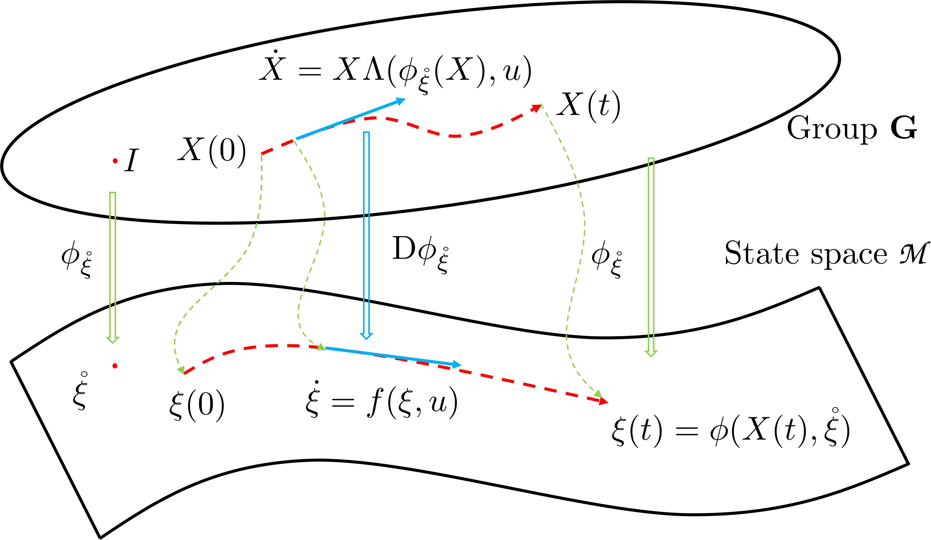
A key advance in equivariant systems theory [MHT20] was the understanding that a lifted system (of an equivariant system on $\mathcal{M}$) can always be written

where $\Lambda:\mathcal{M}\times\mathbb{L}\to\mathfrak{g}$ is termed a lift function [MHT20]. The lifted system formulation (11) encodes internal model dynamics in the standard left invariant form $\dot{X}=X\Lambda$ where $\Lambda\in\mathfrak{g}$ is an element of the Lie-algebra of the Lie-group and $X\Lambda=\mathrm{D}L_{X}\Lambda$ is the left translated tangent vector element of the tangent space of $\mathbf{G}$ at $X$ [BL05, Jur97] where $L_{X}Y=XY$ is the left multiplication on the group. The system lift formulation is more powerful than considering a general $\dot{X}=XU(X,u)$ structure for $U:\mathbf{G}\times\mathbb{L}\to\mathfrak{g}$, since $\Lambda$ as a map defined on $\mathcal{M}\times\mathbb{L}$ ensures that the resulting lifted dynamics are in some sense independent of the stabiliser on $\mathbf{G}$. In particular, if $S\in\stab_{\phi}(\mathring{\xi})$ then $\Lambda(\phi_{\mathring{\xi}}(S),u)=\Lambda(\mathring{\xi},u)$. This ensures that the internal model dynamics of the observer are invariant to left translations $X\mapsto SX$ by the stabiliser

The system lift (eq. 11) is chosen to satisfy the following two conditions:
Pre-image: A necessary and sufficient condition to ensure that solutions of the lifted system project to solutions of the actual system is that

where $\mathrm{D}\phi_{\xi}:\mathfrak{g}\to\mathrm{T}_{\xi}\mathcal{M}$ is the differential of the group action in its group variable, for a given $\xi\in\mathcal{M}$, evaluated at the identity in $\mathbf{G}$ [MTH13, MHT20]. From this it is straightforward to prove that as long as $\phi_{\mathring{\xi}}(\hat{X}(0))=\xi(0)$ then trajectories of (11) project to trajectories of (2) (Figure 3). Since the map $\phi_{\mathring{\xi}}:\mathbf{G}\to\mathcal{M}$ is a submersion the differential $\mathrm{D}\phi_{\mathring{\xi}}:\mathfrak{g}\to\mathrm{T}_{\xi}\mathcal{M}$ is surjective, and it is always possible to define a pre-image $\Lambda(\xi,u)$ of $f(\xi,u)$ in $\mathfrak{g}$ [MTH13]. For a free group action, where the stabiliser is trivial and hence $\phi_{\xi}:\mathbf{G}\to\mathcal{M}$ is invertible, then $\Lambda(\xi,u)=\mathrm{D}\phi_{\xi}^{-1}f(\xi,u)$ and $\Lambda$ is fully defined by (12). Such lifts naturally lead to equivariant system dynamics on the symmetry group. Indeed, for a free action the state-manifold is isomorphic to the symmetry group and the design problem specialises to the case of equivariant observer design on a Lie-group. In general, when the symmetry is not a free action, the pre-image condition (12) is not sufficient to ensure that the lifted system has symmetry properties on the group and without an additional condition leads to issues in the observer analysis.

Equivariance: The second condition required is that the lift respects the symmetry. This condition is encoded as [MHT20]

where $\Ad_{X}:\mathfrak{g}\to\mathfrak{g}$, $U\mapsto XUX^{-1}$, is the adjoint automorphism of the Lie-algebra [BL05, Jur97]. The role of the adjoint here is as the symmetry transformation of the Lie-algebra associated with change of base point $\xi\in\mathcal{M}$. In particular, for any homogeneous space the following diagram is known to commute [BL05, Jur97]

Recalling (12), it is natural to lift the equivariance condition $\mathrm{D}\phi_{X}f(\xi,u)=f(\phi_{X}(\xi),\psi_{X}(u))$ for the system on $\mathcal{M}$ to (13) on the symmetry group. For a free group action, $\Lambda(\xi,u)=\mathrm{D}\phi_{\xi}^{-1}f(\xi,u)$ (from (12)) and equivariance of the lift can be proved by exploiting the equivariance of the system model. However, for groups with non-trivial stabiliser, the condition (13) extends this relationship to the stabiliser. That is, for any $S\in\stab_{\phi}(\xi)$ then (13) becomes $\Ad_{S^{-1}}\Lambda(\xi,u)=\Lambda(\xi,\psi_{S}(u))$ since $\phi_{S}(\xi)=\xi$ by construction. It is only in the unusual case where the stabiliser is a normal subgroup of the symmetry group that this constraint can be ignored without compromising the error dynamics defined in Section 4. Existence of an equivariant lift for any equivariant system is a non-trivial question that was answered in the affirmative in a recent work [MHT20]. There is a construction given in [MHT20] for building a system lift for an arbitrary system based on an iterative process that progressively works through a basis for the input space $\mathbb{L}$. The tricky part is that for each new direction in $\mathbb{L}$, the behaviour of the lift on the stabiliser must be constructed to satisfy the equivariance condition and this influences the next choice of a direction in $\mathbb{L}$. A full discussion is beyond the scope of the present paper beyond noting that, in practice, the most effective way of determining a lift known to the authors is to use (12) and then make educated guesses that can be verified using (13).

The lifted system in the case of the direction kinematics is simply

where $\Omega^{\times}\in\mathfrak{so}(3)$ is in the Lie-algebra of $\mathbf{SO}(3)$, the set of skew-symmetric matrices. The system lift $\Lambda(\eta,\Omega)=\Omega^{\times}$ maps the input directly to the Lie-algebra with no state dependence. The simplicity of this correspondence is both a boon and a curse, as it makes observer design simple for direction kinematics but also hides much of the structure of the general case.

For second order linear kinematics, consider a trajectory $(p(t),v(t))=\phi_{(\alpha,\beta)}(\mathring{p},\mathring{v})$ associated with a lifted system trajectory $(\alpha(t),\beta(t))$ and constant origin $(\mathring{p},\mathring{v})\in\mathbb{R}^{3}\times\mathbb{R}^{3}$. One has

Thus the system lift is $\Lambda((p,v),(w,a)):=(v+w,a)$. Note that the system lift function depends on the system state. To compute the lifted system in terms of $(\alpha,\beta)$ one computes $\frac{\mathrm{d}}{\mathrm{d}t}(\alpha,\beta)=\mathrm{D}L_{(\alpha,\beta)}\Lambda(\phi_{(\alpha,\beta)}(\mathring{p},\mathring{v}),(w,a))$ and sets $w=0$ (corresponding to the actual input) to yield

The offset $\mathring{v}$ in the first equation is important since the symmetry structure of $\beta$ encodes the offset between the true velocity and reference $\beta=v-\mathring{v}$ and not directly the system velocity.

The classical observer error $\tilde{\xi}=\xi-\hat{\xi}\in\mathbb{R}^{m}$ is defined for systems with Euclidean state space $\xi\in\mathbb{R}^{m}$ and where the observer is a copy of the system $\hat{\xi}\in\mathbb{R}^{m}$. This error has been the foundation of observer design both for nonlinear constructive design methods, where $\tilde{\xi}$ is either the primary variable in a Lyapunov construction or is fundamental in the stability analysis, as well as for linearising design methods, where the error $\tilde{\xi}$ is linearised around $\tilde{\xi}=0$. For systems on manifolds, $\tilde{\xi}$ can only be constructed using an atlas of local or embedded coordinates centered around the time-varying state estimate $\hat{\xi}(t)$. This approach to defining an observer error is neither intrinsic nor global. In contrast, a key step in equivariant observer design is the construction of an equivariant error that is both intrinsic and globally defined. Recent work [MHT20] showed that this is only possible by exploiting the symmetry structure of the problem. In particular, there is no error construction $e:\mathcal{M}\times\mathcal{M}\to\mathcal{M}$, $e(\hat{\xi},\xi)\in\mathcal{M}$ between observer and system states at the manifold level [MHT20, Theorem 5.7] that has the nice properties that we will demonstrate with the equivariant error defined below (Eq. (18)). The equivariant error construction (Eq. (14)) overcomes this structural constraint by posing the observer state on the symmetry group. That is, the equivariant error is a map $e:\mathbf{G}\times\mathcal{M}\to\mathcal{M}$, $e(\hat{X},\xi)\in\mathcal{M}$ between an element of the symmetry group $\hat{X}\in\mathbf{G}$ and the system state $\xi\in\mathcal{M}$. This construction motivates the choice to pose the observer state on the symmetry group and in turn motivates the work done in Section 3 to build a lifted system on $\mathbf{G}$ to act as internal model for the observer dynamics.

For an observer state $\hat{X}\in\mathbf{G}$ and a system state $\xi\in\mathcal{M}$ the equivariant error is defined to be

To understand this error recall that the state estimate is given by $\hat{\xi}=\phi_{\hat{X}}(\mathring{\xi})$ for a fixed origin $\mathring{\xi}$. If $e=\mathring{\xi}$ it follows that

Thus, driving the error $e\to\mathring{\xi}$ ensures the that state estimate $\hat{\xi}=\phi_{\hat{X}}(\mathring{\xi})$ converges to the true state $\xi$.

It is instructive to consider the linear kinematics example. The observer state $\hat{X}\in\mathbf{R}^{3}\times\mathbf{R}^{3}$ is an element of the Galilean group. Write $\hat{X}=(\hat{\alpha},\hat{\beta})$, then

Choose $\mathring{\xi}=(0,0)$ to be the origin point in $\mathbb{R}^{3}\times\mathbb{R}^{3}$ and define the state estimate to be $(\hat{p},\hat{v})=\phi_{(0,0)}(\hat{\alpha},\hat{\beta})=(\hat{\alpha},\hat{\beta})$. Substituting into the error yields $e=(p-\hat{p},v-\hat{v})$ the classical linear observer error. Driving $e\to(0,0)$ is the same is driving $\tilde{p}=p-\hat{p}$ and $\tilde{v}=v-\hat{v}$ to zero. The equivariant error construction passes the “pub test” of specialising to the classical linear error in the case where the state space $\mathcal{M}=\mathbb{R}^{m}$ is linear.

The direction kinematics example, however, demonstrates the power of the equivariant error. In this case $\hat{X}=\hat{Q}\in\mathbf{SO}(3)$ and there is no natural origin $\mathring{\xi}=\mathring{\eta}$. Let us choose $\mathring{\eta}=\mathbf{e}_{3}$ in lieu of any better choice. The equivariant error is

If $e=\mathbf{e}_{3}=\hat{Q}\eta$ then $\eta=\hat{Q}^{\top}\mathbf{e}_{3}=\hat{\eta}$ where the second equality is the definition of $\hat{\eta}=\phi_{\hat{Q}}(\mathbf{e}_{3})$. In contrast, the difference in state elements $(\eta-\hat{\eta})$ is not an element of $\mathrm{S}^{2}$ and can only be expressed in a non-intrinsic way in either embedded or local coordinates. More importantly, the equivariant error lives in a neighbourhood of a fixed origin $\mathring{\eta}=\mathbf{e}_{3}$ on the sphere while the coordinates for the difference $(\eta-\hat{\eta})$ must be chosen carefully and changed periodically as $\eta$ and $\hat{\eta}$ move.

For any $\hat{X}$, the equivariant error $e=\phi_{\hat{X}^{-1}}(\xi)\in\mathcal{M}$ is well defined. This opens the door to global analysis of observer convergence, something that is rarely possible for standard observer architectures applied to nonlinear systems on manifolds. Nonlinear observer designs can be designed based on Lyapunov functions $V:\mathcal{M}\to\mathbb{R}_{+}$ written as a function of error coordinates $V(e)$ and centered at the origin $V(\mathring{\xi})=0$. Construction of the Lyapunov functions and design of the observer must be undertaken on a case-by-case basis, however, the resulting observers are inherently globally defined and their basins of attraction are only limited by the construction of the Lyapunov function and topological constraints of the manifold $\mathcal{M}$ [HZT+11, VCSO10, MHV11, HMT+11, THML12, GFJS12, BSO12, IS14, HHMT15, AMB16, HMH16, BAT17, LBHMS17, HHMT15, ZF18, WT19, HTH+19, HTH+20]. For linearisation based observer design, the error dynamics can be linearised at $\mathring{\xi}$ using a single set of local coordinates [BMR06, MS07, MS08, BMR08, BMR09, BMS09, ZTM13, BMGB13, BMAG15, BB15, STMA16, BB17, BB18, LAF19, PC20, vHM20, vGHM20]. The improved regularity of the linearisation (no coordinate changes) leads to improved observer performances as is shown for the equivariant filter design presented in Section 6.

The equivariant error construction allows a principled observer architecture for equivariant systems as shown in Figure 4.

The observer state lies in the symmetry group and uses the internal model provided by the lifted kinematics (11)

Here the correction term $\Delta_{t}:=\Delta_{t}(\hat{X},y)\in\mathfrak{g}$ must be a function of the observed outputs $y$ and the known observer state $\hat{X}$ and remains to be defined. The equivariant error $e$ is generated as a signal and the design goal is to drive $e\to\mathring{\xi}$ asymptotically. In the case that $e\to\mathring{\xi}$ then the state estimate $\hat{\xi}=\phi_{\mathring{\xi}}(\hat{X})$ will converge to the true state $\xi$ (see (15)). The observer state $\hat{X}$ lives in a higher dimensional space $\mathbf{G}$ and its convergence is not characterised directly.

The proposed architecture leads to a clear design principle: to design the correction term $\Delta_{t}$ such that the equivariant error dynamics $e\to\mathring{\xi}$. To do this one must study the dynamics of the equivariant error in detail. It is a straightforward exercise to compute [MHT21]

Formally, the error dynamics are a system defined for $e\in\mathcal{M}$ with two exogenous inputs $u(t)$ and $\hat{X}(t)$ while the correction term can be considered separately as an arbitrary forcing term in the tangent space $\mathrm{T}_{e}\mathcal{M}$. The input $u(t)$ dependence is structural in the problem, indeed, in many robotics problems a persistently exciting input signal is required to ensure observability of the system [THML12]. However, the dependence of the error dynamics on $\hat{X}$ in such an embedded manner will lead to challenges in the analysis. The fact that the evolution of $\hat{X}$ depends in turn on the choice of correction term $\Delta_{t}$ adds additional complexity.

This is where equivariance of the lifted system plays a critical role. Recall that for an equivariant lift $\Ad_{\hat{X}}\Lambda(\xi,u)=\Lambda(\phi_{\hat{X}^{-1}}(\xi),\psi_{\hat{X}^{-1}}(u))$ (see (13)). Factoring the adjoint operator into the dynamics yields

where we introduce the notation

and term this the origin input. The best way to understand $\mathring{u}$ is as a ‘change of basis’ transformation that takes the input $u$ (a velocity measurement) and rewrites it in the correct ‘frame of reference’ to apply to the error kinematics (18). In robotic systems where sensors are mounted on the vehicle then the action $\psi_{\hat{X}^{-1}}$ is typically an explicit change of basis, usually a rotation, that transforms the measurement from the body-fixed-frame to the observers best estimate of the reference frame. For example, in the direction kinematics example $\psi_{\hat{Q}^{\top}}(\Omega)=\hat{Q}\Omega$ can be interpreted as a change of basis for the input $\Omega$ measured in the body-fixed-frame to $\hat{Q}\Omega$ in the (observers best estimate of the) reference frame.

Whereas Eq. (17) are dynamics in two exogenous inputs $\hat{X}$ and $u(t)$ as well as the correction term, the equivariant error dynamics Eq. (18) have a single exogenous input $\mathring{u}(t)$ along with the correction term. Analogous to the general case, the equivariant error dynamics often depend on a persistently exciting input $\mathring{u}(t)$ to ensure observability, particularly for robotic systems. This imposes some constraints on the relative relationship between the observer trajectory and the input, which, at least asymptotically, corresponds to a constraint on the relationship between the system trajectory and the raw input. However, apart from the observability analysis, the fact that $\mathring{u}(t)$ depends on the observer state makes no difference to the observer design. The error dynamics (18) are not autonomous (except in certain special cases [MTH13]), however, the simplicity and elegance of the equation provides a powerful tool in observer design. For non-linear observer design then the global structure of $\Lambda(e,\mathring{u})$ is of interest and there are many systems where this structure has tractable algebraic structure and it is possible to build globally defined non-linear observers [HZT+11, VCSO10, MHV11, HMT+11, THML12, GFJS12, BSO12, IS14, HHMT15, AMB16, HMH16, BAT17, LBHMS17, HHMT15, ZF18, WT19, HTH+19, HTH+20]. For linearising observers then it is the local structure of the error dynamics that are of interest [BMR06, MS07, MS08, BMR08, BMR09, BMS09, ZTM13, BMGB13, BMAG15, BB15, STMA16, BB17, BB18, LAF19, PC20, vHM20, vGHM20]. In this case, the linearisation of the unforced error dynamics in $e$ around $\mathring{\xi}$ are straightforward to compute and provide a powerful model for observer design as we show in Section 6.

References

- [AMB16] Guillaume Allibert, Robert Mahony, and Moses Bangura. Velocity aided attitude estimation for aerial robotic vehicles using latent rotation scaling. In 2016 IEEE International Conference on Robotics and Automation (ICRA), pages 1538–1543, May 2016.
- [AR03] N. Aghannan and P. Rouchon. An intrinsic observer for a class of Lagrangian systems. Automatic Control, IEEE Transactions on, 48(6):936–945, June 2003.
- [BAT17] Soulaimane Berkane, Abdelkader Abdessameud, and Abdelhamid Tayebi. Hybrid global exponential stabilization on SO(3). Automatica, 81:279–285, July 2017.
- [BB15] Axel Barrau and Silvère Bonnabel. Intrinsic Filtering on Lie Groups With Applications to Attitude Estimation. IEEE Transactions on Automatic Control, 60(2):436–449, February 2015.
- [BB16] Axel Barrau and Silvere Bonnabel. An EKF-SLAM algorithm with consistency properties. arXiv:1510.06263, 2016.
- [BB17] A. Barrau and S. Bonnabel. The invariant extended Kalman filter as a stable observer. IEEE Transactions on Automatic Control, 62(4):1797–1812, 2017.
- [BB18] Axel Barrau and Silvère Bonnabel. Invariant Kalman Filtering. Annual Review of Control, Robotics, and Autonomous Systems, 1(1):237–257, 2018.
- [BBB18] Martin Brossard, Silvére Bonnabel, and Axel Barrau. Unscented Kalman Filter on Lie Groups for Visual Inertial Odometry. In 2018 IEEE/RSJ International Conference on Intelligent Robots and Systems (IROS), pages 649–655, October 2018.
- [BBB20] Martin Brossard, Axel Barrau, and Silvère Bonnabel. A Code for Unscented Kalman Filtering on Manifolds (UKF-M). In 2020 IEEE International Conference on Robotics and Automation (ICRA), pages 5701–5708, May 2020.
- [BBC17] Martin Brossard, Silvère Bonnabel, and Jean-Philippe Condomines. Unscented Kalman filtering on Lie groups. In 2017 IEEE/RSJ International Conference on Intelligent Robots and Systems (IROS), pages 2485–2491, September 2017.
- [BL05] F. Bullo and A.D. Lewis. Geometric control of mechanical systems. Springer, 2005.
- [BLB+17] Johannes Berger, Frank Lenzen, Florian Becker, Andreas Neufeld, and Christoph Schnörr. Second-order recursive filtering on the rigid-motion lie group based on nonlinear observations. Journal of Mathematical Imaging and Vision, 58(1):102–129, 2017.
- [BMAG15] Guillaume Bourmaud, Rémi Mégret, Marc Arnaudon, and Audrey Giremus. Continuous-Discrete Extended Kalman Filter on Matrix Lie Groups Using Concentrated Gaussian Distributions. Journal of Mathematical Imaging and Vision, 51(1):209–228, January 2015.
- [BMGB13] Guillaume Bourmaud, Rémi Mégret, Audrey Giremus, and Yannick Berthoumieu. Discrete extended kalman filter on lie groups. In 21st European Signal Processing Conference (EUSIPCO 2013), pages 1–5. IEEE, 2013.
- [BMR06] S. Bonnabel, P. Martin, and P. Rouchon. A non-linear symmetry-preserving observer for velocity-aided inertial navigation. In American Control Conference, Proceedings of The, pages 2910–2914, 2006.
- [BMR08] S. Bonnabel, P. Martin, and P. Rouchon. Symmetry-preserving observers. IEEE Transactions on Automatic Control, 53(11):2514–2526, 2008.
- [BMR09] S. Bonnabel, P. Martin, and P. Rouchon. Non-linear symmetry-preserving observers on Lie groups. IEEE Transactions on Automatic Control, 54(7):1709–1713, 2009.
- [BMS09] Silvère Bonnabel, Philippe Martin, and Erwan Salaün. Invariant Extended Kalman Filter: Theory and application to a velocity-aided attitude estimation problem. In Proceedings of the 48h IEEE Conference on Decision and Control (CDC) Held Jointly with 2009 28th Chinese Control Conference, pages 1297–1304, December 2009.
- [Bon07a] Silvere Bonnabel. Left-invariant extended Kalman filter and attitude estimation. In 2007 46th IEEE Conference on Decision and Control, pages 1027–1032, December 2007.
- [Bon07b] Silvere Bonnabel. Observateurs Asymptotiques Invariant: Theorie et Examples. PhD thesis, Ecole des Mines, Paris, 60 Bld St Michel, Paris, 2007.
- [Bon10] Silvere Bonnabel. A Simple Intrinsic Reduced-Observer for Geodesic Flow. IEEE Transactions on Automatic Control, 55(9):2186–2191, 2010.
- [BR05] Silvère Bonnabel and Pierre Rouchon. Control and observer design for nonlinear finite and infinite dimensional systems. In Lecture Notes in Control and Information Sciences, volume 322, chapter On Invariant Observers, pages 53–67. Springer-Verlag, 2005.
- [BSO12] Pedro Batista, Carlos Silvestre, and Paulo Oliveira. Sensor-Based Globally Asymptotically Stable Filters for Attitude Estimation: Analysis, Design, and Performance Evaluation. IEEE Transactions on Automatic Control, 57(8):2095–2100, August 2012.
- [Cam87] David K Campbell. From Paradigms to Practicalities. Nonlinear Science, page 46, 1987.
- [CBO06] D. Choukroun, I.Y. Bar-Itzhack, and Y. Oshman. Novel quaternion Kalman filter. IEEE Transactions on Aerospace and Electronic Systems, 42(1):174–190, January 2006.
- [CMC07] John L. Crassidis, F. Landis Markley, and Yang Cheng. Nonlinear attitude filtering methods. Journal of Guidance, Control,and Dynamics, 30(1):12–28, 2007.
- [GFJS12] H. F. Grip, T. I. Fossen, T. A. Johansen, and A. Saberi. Attitude Estimation Using Biased Gyro and Vector Measurements With Time-Varying Reference Vectors. IEEE Transactions on Automatic Control, 57(5):1332–1338, May 2012.
- [GM85] Jessy Grizzle and Steven Marcus. The structure of nonlinear control systems possessing symmetries. IEEE Transactions on Automatic Control, 30(3):248–258, 1985.
- [HA18] Minh-Due Hua and Guillaume Allibert. Riccati observer design for pose, linear velocity and gravity direction estimation using landmark position and imu measurements. In 2018 IEEE Conference on Control Technology and Applications (CCTA), pages 1313–1318, 2018.
- [HHMT15] Minh-Duc Hua, Tarek Hamel, Robert Mahony, and Jochen Trumpf. Gradient like Observer Design on the Special Euclidean Group SE(3) with system output on the Projective space. In Procedings of the 54th IEEE Conference on Decision and Control (CDC), pages 2139–2145, 2015.
- [HM06] T. Hamel and R. Mahony. Attitude estimation on based on direct inertial measurements. In Proceedings of the IEEE International Conference on Robotics and Automation (ICRA), pages 2170–2175, April 2006.
- [HMH16] Minh-Duc Hua, Philippe Martin, and Tarek Hamel. Stability analysis of velocity-aided attitude observers for accelerated vehicles. Automatica, 63:11–15, January 2016.
- [HMT+11] Tarek Hamel, Robert Mahony, Jochen Trumpf, Pascal Morin, and Minh-Duc Hua. Homography estimation on the Special Linear Group based on direct point correspondence. In Proceedings of the IEEE Conference on Decision and Control and European Control Conference, Orlando, FL, USA, December 2011.
- [HS18] T. Hamel and C. Samson. Riccati observers for the nonstationary PnP problem. IEEE Transactions on Automatic Control, 63(3):726–741, March 2018.
- [HTH+19] Minh-Duc Hua, Jochen Trumpf, Tarek Hamel, Robert Mahony, and Pascal Morin. Feature-based recursive observer design for homography estimation and its application to image stabilization. Asian Journal of Control, 21(4):1443–1458, 2019.
- [HTH+20] Minh-Duc Hua, Jochen Trumpf, Tarek Hamel, Robert Mahony, and Pascal Morin. Nonlinear observer design on (3) for homography estimation by exploiting point and line correspondences with application to image stabilization. Automatica, 115:10 pages, May 2020.
- [HZT+11] Minh-Duc Hua, Mohammad Zamani, Jochen Trumpf, Robert Mahony, and Tarek Hamel. Observer design on the special euclidean group SE(3). In Proceedings of the IEEE Conference on Decision and Control and European Control Conference, Orlando, FL, USA, December 2011.
- [IS14] Maziar Izadi and Amit Sanyal. Rigid body attitude estimation based on the lagrange–d’alembert principle. Automatica, 50(10):2570–2577, 2014.
- [JAF+15] Berger J., Neufeld A., Becker F., Lenzen F., and Schnörr C. Second order minimum energy filtering on with nonlinear measurement equations. In Scale Space and Variational Methods in Computer Vision. SSVM, volume 9087 of Lecture Notes in Computer Science. Springer, 2015.
- [JMB20] Anant A. Joshi, D. H. S. Maithripala, and Ravi N. Banavar. A bundle framework for observer design on smooth manifolds with symmetry. arXiv:1907.09234, 2020.
- [Jur97] Velimir Jurdjevic. Geometric control theory. Cambridge university press, 1997.
- [KN63] Shoshichi Kobayashi and Katsumi Nomizu. Foundations of differential geometry, volume 1. New York, London, 1963.
- [LAF19] Marc-Antoine Lavoie, Jonathan Arsenault, and James Richard Forbes. An invariant extended filter. In 2019 IEEE 58th Conference on Decision and Control (CDC), pages 7905–7910, 2019.
- [LBHMS17] Florent Le Bras, Tarek Hamel, Robert Mahony, and Claude Samson. Observers for position estimation using bearing and biased velocity information. In Sensing and Control for Autonomous Vehicles, pages 3–23. Springer, 2017.
- [LMS82] E.J. Lefferts, F.L. Markley, and M.D. Shuster. Kalman Filtering for Spacecraft Attitude Estimation. Journal of Guidance, Control, and Dynamics, 5(5):417–429, 1982.
- [LTM10] C. Lageman, J. Trumpf, and R. Mahony. Gradient-like observers for invariant dynamics on a Lie group. IEEE Transactions on Automatic Control, 55(2):367–377, 2010.
- [LWK16] Giuseppe Loianno, Michael Watterson, and Vijay Kumar. Visual inertial odometry for quadrotors on SE(3). In 2016 IEEE International Conference on Robotics and Automation (ICRA), pages 1544–1551, May 2016.
- [Mar03] F. Landis Markley. Attitude Error Representations for Kalman Filtering. Journal of Guidance, Control, and Dynamics, 26(2):311–317, 2003.
- [Mar04] F Landis Markley. Attitude estimation or quaternion estimation? The Journal of the Astronautical Sciences, 52(1):221–238, 2004.
- [May82] Peter S. Maybeck. Stochastic models, estimation and control, v2, volume 2. Academic Press New York, 1982.
- [MBD04] D.H.S. Maithripala, J.M. Berg, and W.P. Dayawansa. An intrinsic observer for a class of simple mechanical systems on a Lie group. In American Control Conference, volume 2, pages 1546–1551, June 2004.
- [MH17] Robert Mahony and Tarek Hamel. A geometric nonlinear observer for simultaneous localisation and mapping. In Conference on Decision and Control, page 6 pages, Melbourne, December 2017.
- [MHP05] R. Mahony, T. Hamel, and J.-M. Pflimlin. Complementary filter design on the special orthogonal group . In Proceedings of the IEEE Conference on Decision and Control (CDC), pages 1477–1484, December 2005.
- [MHP08] R. Mahony, T. Hamel, and J.-M. Pflimlin. Non-linear complementary filters on the special orthogonal group. IEEE Transactions on Automatic Control, 53(5):1203–1218, June 2008.
- [MHT20] Robert Mahony, Tarek Hamel, and Jochen Trumpf. Equivariant Systems Theory and Observer Design. arXiv: https://arxiv.org/abs/2006.08276, 2020.
- [MHT21] Robert Mahony, Tarek Hamel, and Jochen Trumpf. An homogeneous space geometry for simultaneous localisation and mapping. Annual Reviews in Control, June 2021.
- [MHV11] S.O. Madgwick, A.J. Harrison, and R. Vaidyanathan. Estimation of imu and marg orientation using a gradient descent algorithm. In International Conference on Rehabilitation Robotics (ICORR2011), page 32, 2011.
- [MPHS05] N. Metni, J.-M. Pflimlin, T. Hamel, and P. Soueres. Attitude and gyro bias estimation for a flying UAV. In 2005 IEEE/RSJ International Conference on Intelligent Robots and Systems, pages 1114–1120, 2005.
- [MS07] Ph. Martin and E. Salaün. Invariant observers for attitude and heading estimation from low-cost inertial and magnetic sensors. In Proceedings of the 46th IEEE Conference on Decision and Control, pages 1039–1045, 2007.
- [MS08] Philippe Martin and Erwan Salaün. An invariant observer for earth-velocity-aided attitude heading reference systems. IFAC Proceedings Volumes, 41(2):9857–9864, 2008.
- [MT21] Robert Mahony and Jochen Trumpf. Equivariant filter design for kinematic systems on lie groups. In Proceedings of Symposium on Mathematical Theory of Networks and Systems (MTNS2020), 2021.
- [MTH13] Robert Mahony, Jochen Trumpf, and Tarek Hamel. Observers for kinematic systems with symmetry. In IFAC Proceedings Volumes, volume 46, pages 617–633. Elsevier, 2013.
- [Nv85] Henk Nijmeijer and AJ van der Schaft. Partial symmetries for nonlinear systems. Mathematical systems theory, 18(1):79–96, 1985.
- [NvHM20] Yonhon Ng, Pieter van Goor, Tarek Hamel, and Robert Mahony. Equivariant systems theory and observer design for second order kinematic systems on matrix lie groups. In Proceedings of the IEEE Conference on Decision and Control (CDC), 2020.
- [NvMH19] Yonhon Ng, Pieter van Goor, Robert Mahony, and Tarek Hamel. Attitude observation for second order attitude kinematics. In Proceedings of the IEEE Conference on Decision and Control (CDC), page 6 pages, 2019.
- [PC20] Karmvir Singh Phogat and Dong Eui Chang. Invariant extended kalman filter on matrix lie groups. Automatica, 114:108812, 2020.
- [RSB99] S.I. Roumeliotis, G.S. Sukhatme, and G.A. Bekey. Circumventing dynamic modeling: Evaluation of the error-state Kalman filter applied to mobile robot localization. In Proceedings 1999 IEEE International Conference on Robotics and Automation (Cat. No.99CH36288C), volume 2, pages 1656–1663 vol.2, May 1999.
- [RSB05] Peter D. Joseph Richard S. Bucy. Filtering for stochastic processes with applications to guidance, volume 26. American Mathematical Society, 2005.
- [Sal91] S. Salcudean. A globally convergent angular velocity observer for rigid body motion. IEEE Transactions on Automatic Control, 46, no 12:1493–1497, 1991.
- [Sol17] Joan Solà. Quaternion kinematics for the error-state Kalman filter. arXiv:1711.02508 [cs], November 2017.
- [STMA16] Alessandro Saccon, Jochen Trumpf, Robert Mahony, and A. Pedro Aguiar. Second-order-optimal minimum-energy filter on lie groups. IEEE Transactions on Automatic Control, 61(10):2906–2919, October 2016.
- [THML12] Jochen Trumpf, Tarek Hamel, Robert Mahony, and Christian Lageman. Analysis of non-linear attitude observers for time-varying reference measurements. IEEE Transactions on Automatic Control, 57(11):2789–2800, 2012.
- [TS03] J. Thienel and R. M. Sanner. A coupled nonlinear spacecraft attitude controller and observer with an unknow constant gyro bias and gyro noise. IEEE Transactions on Automatic Control, 48(11):2011–2015, November 2003.
- [van81] Arjan van der Schaft. Symmetries and conservation laws for Hamiltonian systems with inputs and outputs: A generalization of Noether’s theorem. Systems & Control Letters, 1(2):108–115, 1981.
- [VCSO10] J.F. Vasconcelos, R. Cunha, C. Silvestre, and P. Oliveira. A nonlinear position and attitude observer on SE(3) using landmark measurements. Systems & Control Letters, 59(3-4):155–166, March 2010.
- [VF01] B. Vik and T. Fossen. A nonlinear observer for GPS and INS integration. In Proceedings of the 40th IEEE Conference on Decision and Control, 2001.
- [vGHM20] Pieter van Goor, Tarek Hamel, and Robert Mahony. Equivariant filter (EqF). arXiv preprint arXiv:2010.14666, 2020.
- [vHM20] Pieter van Goor, Tarek Hamel, and Robert Mahony. Equivariant filter (EqF): A general filter design for systems on homogeneous spaces. In Proceedings of the Conference on Decision and Control, pages 5401–5408, 2020.
- [vM21] Pieter van Goor and Robert Mahony. An Equivariant Filter for Visual Inertial Odometry. In Proceedigns of the IEEE International Conference on Robotics and Automation (ICRA2021), 2021.
- [vMHT19] Pieter van Goor, Robert Mahony, Tarek Hamel, and Jochen Trumpf. A geometric observer design for visual localisation and mapping. In Proceedings of the IEEE Conference on Decision and Control, pages 2543–2549, 2019.
- [vMHT20] Pieter van Goor, Robert Mahony, Tarek Hamel, and Jochen Trumpf. An observer design for visual simultaneous localisation and mapping with output equivariance. In Procedings of the IFAC World Congress, volume 53, pages 9560–9565, 2020.
- [WBT21] Miaomiao Wang, Soulaimane Berkane, and Abdelhamid Tayebi. Nonlinear observers design for vision-aided inertial navigation systems. IEEE Transactions on Automatic Control, page 16, 2021.
- [WT19] Miaomiao Wang and Abdelhamid Tayebi. Hybrid pose and velocity-bias estimation on using inertial and landmark measurements. IEEE Transactions on Automatic Control, 64(8):3399–3406, 2019.
- [ZF18] David Evan Zlotnik and James Richard Forbes. Gradient-based observer for simultaneous localization and mapping. IEEE Transactions on Automatic Control, 63(12):4338–4344, 2018.
- [ZTM13] M. Zamani, J. Trumpf, and R. Mahony. Minimum-energy filtering for attitude estimation. IEEE Transactions on Automatic Control, 58(11):2917–2921, November 2013.
- [ZWS+17] Teng Zhang, Kanzhi Wu, Jingwei Song, Shoudong Huang, and Gamini Dissanayake. Convergence and Consistency Analysis for a 3-D Invariant-EKF SLAM. IEEE Robotics and Automation Letters, 2(2):733–740, April 2017.