On the Parallel I/O Optimality of Linear Algebra Kernels: Near-Optimal Matrix FactorizationsConference: Technical Report; 2021;

To model algorithmic I/O complexity, we start with a model of a sequential machine equipped with a two-level deep memory hierarchy. We then outline the parallel machine model.

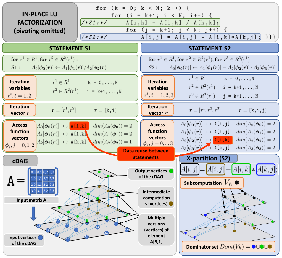
We consider a general class of programs that operate on multidimensional arrays. Array elements can be loaded from slow to fast memory, stored from fast to slow memory, and computed inside fast memory. These elements have versions that are incremented every time they are updated. We model the program execution as a computational directed acyclic graph (cDAG, details in Section 2.3), where each vertex corresponds to a different version of an array element. Thus, for a statement $A[i,j]\leftarrow f(A[i,j])$, a vertex corresponding to $A[i,j]$ after applying $f$ is different from a vertex corresponding to $A[i,j]$ before applying $f$. In a cDAG, this is expressed as an edge from vertex $A[i,j]$ before $f$ to vertex $A[i,j]$ after $f$. Initial versions of each element do not have any incoming edges and thus form the cDAG inputs. The distinction between elements and vertices is important for our I/O lower bounds analysis, as we will investigate how many vertices are computed for a given number of loaded vertices.

An input program is a collection of statements $S$ enclosed in loop nests, each of the following form (we use the loop nest notation introduced by Dinh and Demmel (Dinh and Demmel 2020)):

Each loop has an associated iteration variable $\psi^{t}$ that iterates over its domain $\psi^{t}\in\mathcal{D}^{t}$. All $l$ iteration variables form the iteration vector $\bm{\psi}=[\psi^{1},\dots,\psi^{l}]$. Array elements are accessed by an access function vector $\bm{\phi_{j}}=[\phi_{j}^{1},\dots,\phi_{j}^{dim(A_{j})}]$ that maps $dim(A_{j})$ iteration variables to a unique element in array $A_{j}$ (note that the access function vector is injective). Only vertices associated with the newest element versions can be referenced. Furthermore, a given vertex can be referenced by only one access function vector per statement. We refer to this as the disjoint access property. The access dimension of $A_{j}(\bm{\phi}_{j})$, denoted $dim(A_{j}(\bm{\phi}_{j}))$, is the number of different iteration variables present in $\bm{\phi}_{j}$. We call such programs Disjoint Access Array Programs.

Example: Consider statement $S1$ of LU factorization (Figure 3). The loop nest depth is $l=2$, with two iteration variables $\psi^{1}=$ k and $\psi^{2}=$ i forming the iteration vector $\bm{\psi}=$ [k, i]. For access $A[k,k]$, the access function vector $\bm{\phi}_{j}=[k,k]$ is a function of only one iteration variable $k$. Therefore, $dim(A_{j})=2$, but $dim(A_{j}(\bm{\phi_{j}}))=1$.

We now establish the relationship between DAAP and the red-blue pebble game - a powerful abstraction for deriving lower bounds and optimal schedules of cDAG evaluation.

Each execution of statement $S$ is associated with the iteration vector value $\bm{\psi}=[\psi^{1},\dots,\psi^{l}]\in\mathbb{N}^{l}$ representing the current iteration, that is, the values of iteration variables $\psi^{1}$$,\dots,$$\psi^{l}$. Each subcomputation $H$ is uniquely defined by all iteration vectors’ values associated with vertices pebbled in $H=\{\bm{\psi}_{1},\dots,\bm{\psi}_{|H|}\}$. For each iteration variable $\psi^{t}$, $t=1,\dots,l$, denote the set of all values that $\psi^{t}$ takes during $H$ as $D^{t}$. We define $\bm{D}=[D^{1},\dots,D^{t}]\subseteq\mathcal{\bm{D}}$ as the iteration domain of subcomputation $H$.

Furthermore, recall that each input access $A_{j}[\bm{\phi_{j}}(\bm{\psi})]$ is uniquely defined by $dim(\bm{\phi}_{j})$ iteration variables $\psi_{j}^{1},\dots,\psi_{j}^{dim(\bm{\phi}_{j})}$. Denote the set of all values each of $\psi_{j}^{k}$ takes during $H$ as $D^{k}_{j}$. Given $\bm{D}$, we also denote the number of different vertices that are accessed from each input array $A_{j}$ as $|A_{j}(\bm{D})|$.

We now state the lemma which bounds $|H|$ by the iteration sets’ sizes $|D^{t}|$ (the intuition behind the lemma is depicted in Figure 4):

To prove it, we now introduce two auxiliary lemmas:

Now, given $\bm{D}$, we want to assess how many different vertices are accessed for each input array $A_{j}$. Recall that this number is denoted as access size $|A_{j}(\bm{D})|$.

We will apply the same combinatorial reasoning to $A_{j}(\bm{D})$. For each access $A_{j}[\bm{\phi}_{j}(\bm{\psi})]$, each one of $\psi_{j}^{k}$, $k=1,\dots,dim(\bm{\phi}_{j})$ iteration variables loops over set $R_{h,j}^{k}$ during subcomputation $H$. We can thus bound size of $A_{j}(\bm{D})$ similarly to Lemma 4:

Dominator set. Input vertices $A_{1},\dots,A_{m}$ form a dominator set of vertices $A_{0}$, because any path from graph inputs to any vertex in $A_{0}$ must include at least one vertex from $A_{1},\dots,A_{m}$. This is also the minimum dominator set, because of the disjoint access property (Section 2.2): any path from graph inputs to any vertex in $A_{0}$ can include at most one vertex from $A_{1},\dots,A_{m}$.

Now we prove that to maximize $|H|$, inequalities 1 and 2 must be tight (become equalities).

From proof of Lemma 4 it follows that $|H|$ is maximized when iteration vector $\bm{\psi}$ takes all possible combinations of iteration variables $\psi^{t}\in D^{t}$ during $H$. But, as we visit each combination of all $l$ iteration variables, for each access $A_{j}$ every combination of its $[\psi_{j}^{1},\dots,\psi_{j}^{dim(\bm{\phi}_{j})}]$ iteration variables is also visited. Therefore, for every $j=1,\dots,m$, each access size $|A_{j}(\bm{\mathcal{D}})|$ is maximized (Lemma 5), as access functions are injective, which implies that for each combination of $[\psi_{j}^{1},\dots,\psi_{j}^{dim(\bm{\phi}_{j})}]$, there is one access to $A_{j}$. $\prod_{t=1}^{l}|R_{h}^{t}|$ is then the upper bound on $|H|$, and its tightness implies that all bounds on access sizes $|A_{j}(\bm{\mathcal{D}})|\leq\prod_{k=1}^{dim(\bm{\phi}_{j})}|D^{k}_{j}|$ are also tight. ∎

Denoting $H_{max}=\argmax_{H\in\mathcal{P}(X)}|H|$ as the largest subcomputation among all valid $X$-partitions, we use Lemma 3 and combine it with the dominator set constraint from Section 2.3.3. Note that all access set sizes are strictly positive integers $|{D}^{t}|\in\mathbb{N}_{+},t=1,\dots,l$. Otherwise, if any of the sets is empty, no computation can be performed. However, as we only want to find the bound on the number of I/O operations, we relax the integer constraints and replace them with $|D^{t}|\geq 1$. Then, we formulate finding $\chi(X)$ (Lemma 2) as the following optimization problem:

We then find $|H_{max}|=\chi(X)$ as a function of $X$ using Karush –Kuhn–Tucker (KKT) conditions (Kuhn and Tucker 2014). Next, we solve

Denoting $X_{0}$ as the solution to Equation (4), we finally obtain

Example: Consider Figure 5. In a), each compute vertex $C[i,j]$ has two input vertices: $A[i,j]$ with out-degree 1, and $b[j]$ with out-degree $n$, thus $u=1$. As both array $A$ and vector $b$ start in the slow memory (having blue pebbles on each vertex), for each computed vertex from $C$, at least one vertex from $A$ has to be loaded, therefore $\rho\leq 1$. In b), each computation needs two out-degree 1 vertices, one from vector $a$ and one from vector $b$, resulting in $u=2$. Thus, $\rho\leq\frac{1}{2}$.

Consider two statements $S$ and $T$ that share one input array $A_{i}$. Let $|A_{i}(\bm{R}_{S})|$ denote the total number of accesses to $A_{i}$ during the I/O optimal execution of a program that contains only statement $S$. Naturally, $|A_{i}(\bm{R}_{T})|$ denotes the same for a program containing only $T$. Define $Reuse(A_{i})\coloneqq\min\{|A_{i}(\bm{R}_{S})|,|A_{i}(\bm{R}_{T})|\}$. We then have:

The reuse size is defined as $Reuse(A_{i})=\min\{|A_{i}(\bm{R}_{S})|,$ $|A_{i}(\bm{R}_{T})|\}$. Now, how to find $|A_{i}(\bm{R}_{S})|$ and $|A_{i}(\bm{R}_{T})|$?

Observe that $|A_{i}(\bm{R}_{S})|$ is a property of $G_{S}$, that is, the cDAG containing statement $S$ only. Denote the I/O optimal schedule parameters of $G_{S}$: $V^{S}_{max}$, $X^{S}_{0}$, and $|A_{i}(\bm{R}^{S}_{max}(X^{S}_{0}))|$ (Section 3.2). Similarly, for $G_{T}$: $V^{T}_{max}$, $X^{T}_{0}$, and $|A_{i}(\bm{R}^{T}_{max}(X^{T}_{0}))|$. We now derive: 1) at least how many subcomputations does the optimal schedule have: $s\geq\frac{|V|}{|H_{max}|}$, 2) at least how many accesses to $A_{i}$ are performed per optimal subcomputation $|A_{i}(\bm{R}_{max}(X_{0}))|$. Then:

Note that $Reuse(A_{i})$ is an overapproximation of the actual reuse. Since finding the optimal schedule is PSPACE-complete (Liu 2018), we conservatively assume that only the minimum number of loads from $A_{i}$ is performed. Thus, Lemma 7 generalizes to any number of statements $S_{1},\dots,S_{w}$ sharing array $A_{i}$ — the total number of loads from $A_{i}$ is lower-bounded by a maximum number of loads from $A_{i}$ among $S_{j}$, $\max_{j=1,\dots,w}|A_{i}(\bm{R}_{S_{j}})|$.

Consider the case where the output $A_{0}$ of statement $S$ is also the input $B_{j}$ of statement $T$. Furthermore, consider subcomputation $H$ of statement $T$ (and its associated iteration domain $\bm{{D}}$). Any path from the graph inputs to vertices in $B_{0}(\bm{{D}})$ must pass through vertices in $B_{j}(\bm{{D}})$. The following question arises: Is there a smaller set of vertices $B_{j}^{\prime}(\bm{{D}})$, $|B_{j}^{\prime}(\bm{{D}})|<|B_{j}(\bm{{D}})|$ that every path from graph inputs to $B_{j}(\bm{{D}})$ must pass through?

Let $\rho_{S}$ denote computational intensity of statement $S$. With that, we can state the following lemma:

Similarly to case I, this result also generalizes to multiple “consumer” statements that reuse the same output array of a “producer” statement, as well as any combination of input and output reuse for multiple arrays and statements. Since the actual I/O optimal schedule is unknown, the general strategy to ensure correctness of our lower bound is to consider each pair of interacting statements separately as one of these two cases. Since both Lemma 7 and 8 overapproximate the reuse, the final bound may not be tight - the more inter-statement reuse, the more overapporixmation is needed. Still, this method can be successfully applied to derive tight I/O lower bounds for many linear algebra kernels, such as matrix factorizations, tensor products, or solvers.

In our I/O lower bound analysis we omit the row pivoting, since swapping rows can increase the I/O cost by at most $N^{2}$, which is the cost of permuting the entire matrix. However, the total I/O cost of the LU factorization is $\mathcal{O}(N^{3}/\sqrt{M})$ (Solomonik and Demmel 2011).

LU factorization (without pivoting) contains two statements (Figure 3). Observe that we can use Lemma 6 (out-degree one vertices) for statement $S1:$ A[i,k] = A[i,k] / A[k,k]. The loop nest depth is $l_{S1}=2$, with iteration variables $\psi^{1}=$ k and $\psi^{2}=$ i. The dimension of the access function vector (k,k) is 1, revealing potential for data reuse: every input vertex A[k,k] is accessed $N-k$ times and used to compute vertices A[i,k], $k+1<=i<N$. However, the access function vector (i,k) has dimension 2; therefore, every compute vertex has one direct predecessor with out-degree one, which is the previous version of element A[i,k]. Using Lemma 6, we therefore have $\rho_{S1}\leq 1$.

We now proceed to statement $S2:$ A[i,j] = A[i,j] - A[i,k] * A[k,j]. Let $|D^{k}|=K$, $|D^{i}|=I$, $|D^{j}|=J$. Observe that there is an output reuse (Section 4.2 and Figure 3, red arrow) of A[i,k] between statements $S1$ and $S2$. We therefore have the following access size in statement S2: $|A_{2}(\bm{D}_{S2})|=|$ A[i,k]$|=\frac{IK}{\rho_{S1}}\geq IK$ (Equation 7). Note that in this case where the computational intensity is $\rho_{S1}\leq 1$, the output reuse does not change the access size $|A_{2}(\bm{D}_{S2})|$ of statement $S2$. This follows the intuition that it is not beneficial to recompute vertices if the recomputation cost is higher than loading it from the memory. Denoting $H_{S2}$ as the maximal subcomputation for statement $S2$ over the subcomputation domain $\bm{D}$, we have the following (Lemma 3):

• •

  $|H_{S2}|=KIJ$

• •

  $|A_{1}(\bm{D})|=|$ A[i,j] $|=IJ$

• •

  $|A_{2}(\bm{D})|=|$ A[i,k] $|=IK$

• •

  $|A_{3}(\bm{D})|=|$ A[k,j] $|=KJ$

• •

  $|\mathit{Dom}(H_{S2})|=|A_{1}(\bm{D})|+|A_{2}(\bm{D})|+|A_{3}(\bm{D})|=IJ+IK+KJ$

We then solve the optimization problem from Section 3.2:

Which gives $|H_{S2}|=\chi(X)=\Big(\frac{X}{3}\Big)^{\frac{3}{2}}$ for $K=I=J=\Big(\frac{X}{3}\Big)^{\frac{1}{2}}$. Then, we find $X_{0}$ that minimizes the expression $\rho_{S2}(X)=\frac{|H_{max}|}{X-M}$ (Equation 4), yielding $X_{0}=3M$. Plugging it into $\rho_{S2}(X)$, we conclude that the maximum computational intensity of $S2$ is bounded by $\rho_{S2}\leq\sqrt{M}/2$.

We bounded the maximum computational intensities $\rho_{S1}$ and $\rho_{S2}$, that is, the minimum number of I/O operations to compute vertices belonging to statements $S1$ and $S2$. As the last step, we find the total number of compute vertices for each statement: $|V_{1}|=\sum_{k=1}^{N}(N-k-1)=N(N-1)/2$, and $|V_{2}|=\sum_{k=1}^{N}\sum_{i=k+1}^{N}(N-k-1)=N(N-1)(N-2)/3$. Using Lemmas 1 (bounding I/O cost with the computational intensity) and 9 (I/O cost of the parallel machine), the parallel I/O lower bound for LU factorization is therefore

Previously, Solomonik et al. (Solomonik and Demmel 2011) established the asymptotic I/O bound for sequential execution $Q=\mathcal{O}(N^{3}/\sqrt{M})$. Recently, Olivry et al. (Olivry et al. 2020) derived a tight leading term constant $Q\geq 2N^{3}/(3\sqrt{M})$. To the best of our knowledge, our result is the first non-asymptotic bound for parallel execution. The generalization from the sequential to the parallel bound is straightforward. Note, however, that this is only the case due to our pebble-based execution model, and it may thus not apply to other parallel machine models.

We proceed analogously to our derivation of the LU I/O bound — here we just briefly outline the steps. The algorithm contains three statements (Listing ). For statements $S1$ and $S2$, we can again use Lemma 6 (out-degree-one vertices). For $S1:$ L(k,k) = sqrt(L(k,k)), the loop nest depth is $l_{1}=1$, we have a single iteration variable $\psi^{1}=$ k, and a single input array $A_{1}=$ L with the access function $\phi_{1}(\bm{\psi})=$(k,k). Since there is only one iteration variable present in $\phi_{1}$, we have $dim(\phi_{1})=1=l_{1}$. Therefore, for every compute vertex $v$ we have one direct predecessor, which is the previous version of element L(k,k). We conclude that $\rho_{S1}\leq 1$ and $|V_{S1}|=N$.

For statement $S2:$ L(i,k) = (L(i,k)) / L(k,k), we also have output reuse of L(k,k) between statements $S2$ and $S1$. However, as with the output reuse considered in the LU analysis, the computational intensity is $\rho_{S1}\leq 1$. Therefore, it does not change the dominator set size of $S2$. We then use the same reasoning as for the corresponding statement $S1$ in LU factorization, yielding $\rho_{S2}\leq 1$.

References

- (1)
- Aggarwal and Vitter (1988) Alok Aggarwal and S Vitter, Jeffrey. 1988. The input/output complexity of sorting and related problems. Commun. ACM 31, 9 (1988), 1116–1127.
- Agullo et al. (2011a) Emmanuel Agullo, Cédric Augonnet, Jack Dongarra, Mathieu Faverge, Julien Langou, Hatem Ltaief, and Stanimire Tomov. 2011a. LU factorization for accelerator-based systems. In 2011 9th IEEE/ACS International Conference on Computer Systems and Applications (AICCSA). IEEE, 217–224.
- Agullo et al. (2010) Emmanuel Agullo, Cédric Augonnet, Jack Dongarra, Hatem Ltaief, Raymond Namyst, Samuel Thibault, and Stanimire Tomov. 2010. Faster, Cheaper, Better – a Hybridization Methodology to Develop Linear Algebra Software for GPUs. In GPU Computing Gems, Wen mei W. Hwu (Ed.). Vol. 2. Morgan Kaufmann. https://hal.inria.fr/inria-00547847
- Agullo et al. (2011b) Emmanuel Agullo, Jack Dongarra, Bilel Hadri, Jakub Kurzak, Julie Langou, Julien Langou, Hatem Ltaief, Piotr Luszczek, and Asim YarKhan. 2011b. PLASMA Users’ Guide. Parallel Linear Algebra Software for Multicore Architectures. Rapport technique, Innovative Computing Laboratory, University of Tennessee (2011).
- Alwen and Serbinenko (2015) Joël Alwen and Vladimir Serbinenko. 2015. High parallel complexity graphs and memory-hard functions. In Proceedings of the forty-seventh annual ACM symposium on Theory of computing. 595–603.
- Anderson et al. (1999) Edward Anderson, Zhaojun Bai, Christian Bischof, Susan Blackford, Jack Dongarra, Jeremy Du Croz, Anne Greenbaum, Sven Hammarling, Alan McKenney, and Danny Sorensen. 1999. LAPACK Users’ guide. Vol. 9. Siam.
- Ballard et al. (2010) Grey Ballard, James Demmel, Olga Holtz, and Oded Schwartz. 2010. Communication-optimal parallel and sequential Cholesky decomposition. SIAM Journal on Scientific Computing 32, 6 (2010), 3495–3523.
- Ballard et al. (2011) Grey Ballard, James Demmel, Olga Holtz, and Oded Schwartz. 2011. Minimizing communication in numerical linear algebra. SIAM J. Matrix Anal. Appl. 32, 3 (2011), 866–901.
- Benabderrahmane et al. (2010) Mohamed-Walid Benabderrahmane, Louis-Noël Pouchet, Albert Cohen, and Cédric Bastoul. 2010. The polyhedral model is more widely applicable than you think. In International Conference on Compiler Construction. Springer, 283–303.
- Blackford et al. (1997) L. S. Blackford, J. Choi, A. Cleary, E. D’Azevedo, J. Demmel, I. Dhillon, J. Dongarra, S. Hammarling, G. Henry, A. Petitet, K. Stanley, D. Walker, and R. C. Whaley. 1997. ScaLAPACK Users’ Guide. Society for Industrial and Applied Mathematics, Philadelphia, PA.
- Bondhugula et al. (2008) Uday Bondhugula, Muthu Baskaran, Sriram Krishnamoorthy, J. Ramanujam, Atanas Rountev, and P. Sadayappan. 2008. Automatic Transformations for Communication-Minimized Parallelization and Locality Optimization in the Polyhedral Model. Springer Berlin Heidelberg, Berlin, Heidelberg, 132–146. https://doi.org/10.1007/978-3-540-78791-4_9
- Bosilca et al. (2011) G. Bosilca, A. Bouteiller, A. Danalis, M. Faverge, A. Haidar, T. Herault, J. Kurzak, J. Langou, P. Lemarinier, H. Ltaief, P. Luszczek, A. YarKhan, and J. Dongarra. 2011. Flexible Development of Dense Linear Algebra Algorithms on Massively Parallel Architectures with DPLASMA. In 2011 IEEE International Symposium on Parallel and Distributed Processing Workshops and Phd Forum. 1432–1441.
- Bruno and Sethi (1976) John Bruno and Ravi Sethi. 1976. Code generation for a one-register machine. Journal of the ACM (JACM) 23, 3 (1976), 502–510.
- Choi et al. (1996) J. Choi et al. 1996. ScaLAPACK: a portable linear algebra library for distributed memory computers — design issues and performance. Comp. Phys. Comm. (1996).
- Christ et al. (2013) Michael Christ, James Demmel, Nicholas Knight, Thomas Scanlon, and Katherine Yelick. 2013. Communication lower bounds and optimal algorithms for programs that reference arrays–Part 1. arXiv preprint arXiv:1308.0068 (2013).
- Cray (2020) Cray. 2020. LibSci: Cray Scientific Libraries. (2020). https://olcf.ornl.gov/software_package/libsci/
- Darte (1999) Alain Darte. 1999. On the complexity of loop fusion. In 1999 International Conference on Parallel Architectures and Compilation Techniques (Cat. No. PR00425). IEEE, 149–157.
- Del Ben et al. (2015) Mauro Del Ben et al. 2015. Enabling simulation at the fifth rung of DFT: Large scale RPA calculations with excellent time to solution. Comp. Phys. Comm. (2015).
- Del Ben et al. (2013) Mauro Del Ben, Jurg Hutter, and Joost VandeVondele. 2013. Electron correlation in the condensed phase from a resolution of identity approach based on the Gaussian and plane waves scheme. Journal of chemical theory and computation 9, 6 (2013), 2654–2671.
- Demmel and Dinh (2018) James Demmel and Grace Dinh. 2018. Communication-optimal convolutional neural nets. arXiv preprint arXiv:1802.06905 (2018).
- Demmel and Rusciano (2016) James Demmel and Alex Rusciano. 2016. Parallelepipeds obtaining HBL lower bounds. arXiv preprint arXiv:1611.05944 (2016).
- Dennard et al. (1974) Robert H Dennard, Fritz H Gaensslen, Hwa-Nien Yu, V Leo Rideout, Ernest Bassous, and Andre R LeBlanc. 1974. Design of ion-implanted MOSFET’s with very small physical dimensions. IEEE Journal of Solid-State Circuits 9, 5 (1974), 256–268.
- Dinh and Demmel (2020) Grace Dinh and James Demmel. 2020. Communication-Optimal Tilings for Projective Nested Loops with Arbitrary Bounds. arXiv preprint arXiv:2003.00119 (2020).
- Dongarra et al. (2014) Jack Dongarra, Mathieu Faverge, Hatem Ltaief, and Piotr Luszczek. 2014. Achieving numerical accuracy and high performance using recursive tile LU factorization with partial pivoting. Concurrency and Computation: Practice and Experience 26, 7 (2014), 1408–1431.
- Dongarra and Luszczek (2011) Jack Dongarra and Piotr Luszczek. 2011. TOP500. Springer US, Boston, MA, 2055–2057. https://doi.org/10.1007/978-0-387-09766-4_157
- Elango et al. (2013) V. Elango et al. 2013. Data access complexity: The red/blue pebble game revisited. Technical Report.
- Feautrier (1992) Paul Feautrier. 1992. Some efficient solutions to the affine scheduling problem. I. One-dimensional time. International journal of parallel programming 21, 5 (1992), 313–347.
- Gates et al. (2019) Mark Gates, Jakub Kurzak, Ali Charara, Asim YarKhan, and Jack Dongarra. 2019. SLATE: design of a modern distributed and accelerated linear algebra library. In Proceedings of the International Conference for High Performance Computing, Networking, Storage and Analysis. 1–18.
- Grigori et al. (2008) Laura Grigori, James W Demmel, and Hua Xiang. 2008. Communication avoiding Gaussian elimination. In SC’08: Proceedings of the 2008 ACM/IEEE Conference on Supercomputing. IEEE, 1–12.
- Haidar et al. (2018) Azzam Haidar, Stanimire Tomov, Jack Dongarra, and Nicholas J Higham. 2018. Harnessing GPU tensor cores for fast FP16 arithmetic to speed up mixed-precision iterative refinement solvers. In SC18: International Conference for High Performance Computing, Networking, Storage and Analysis. IEEE, 603–613.
- Hoefler et al. (2015) T. Hoefler et al. 2015. Remote Memory Access Programming in MPI-3. TOPC (2015).
- Hutter ([n. d.]) Edward Hutter. [n. d.]. Communication-Avoiding Parallelism-Increasing maTrix fActorization Library. ([n. d.]). https://github.com/huttered40/capital
- Hutter and Solomonik (2019) Edward Hutter and Edgar Solomonik. 2019. Communication-avoiding Cholesky-QR2 for rectangular matrices. In 2019 IEEE International Parallel and Distributed Processing Symposium (IPDPS). IEEE, 89–100.
- Intel (2020) Intel. 2020. Math Kernel Library. (2020). https://software.intel.com/en-us/mkl
- Invernizzi et al. (2021) Alberto Invernizzi, Teodor Nikolov, Lara Querciagrossa, and Raffaele Solcà. 2021. Distributed Linear Algebra with (HPX) Futures (forthcoming). In Proceedings of the Platform for Advanced Scientific Computing Conference.
- Irony et al. (2004) Dror Irony et al. 2004. Communication Lower Bounds for Distributed-memory Matrix Multiplication. JPDC (2004).
- Jia-Wei and Kung (1981) Hong Jia-Wei and Hsiang-Tsung Kung. 1981. I/O complexity: The red-blue pebble game. In STOC.
- Kabić et al. (2021) Marko Kabić, Simon Pintarelli, Anton Kozhevnikov, and Joost VandeVondele. 2021. COSTA: Communication-Optimal Shuffle and Transpose Algorithm with Process Relabeling. In International Conference on High Performance Computing. Springer, 217–236.
- Karp (1988) Richard M Karp. 1988. A survey of parallel algorithms for shared-memory machines. (1988).
- Kestor et al. (2013) Gokcen Kestor, Roberto Gioiosa, Darren J Kerbyson, and Adolfy Hoisie. 2013. Quantifying the energy cost of data movement in scientific applications. In 2013 IEEE international symposium on workload characterization (IISWC). IEEE, 56–65.
- Knüpfer et al. (2012) Andreas Knüpfer, Christian Rössel, Dieter an Mey, Scott Biersdorff, Kai Diethelm, Dominic Eschweiler, Markus Geimer, Michael Gerndt, Daniel Lorenz, Allen Malony, Wolfgang E. Nagel, Yury Oleynik, Peter Philippen, Pavel Saviankou, Dirk Schmidl, Sameer Shende, Ronny Tschüter, Michael Wagner, Bert Wesarg, and Felix Wolf. 2012. Score-P: A Joint Performance Measurement Run-Time Infrastructure for Periscope,Scalasca, TAU, and Vampir. In Tools for High Performance Computing 2011, Holger Brunst, Matthias S. Müller, Wolfgang E. Nagel, and Michael M. Resch (Eds.). Springer Berlin Heidelberg, Berlin, Heidelberg, 79–91.
- Krishnamoorthy and Menon (2013) Aravindh Krishnamoorthy and Deepak Menon. 2013. Matrix inversion using Cholesky decomposition. In 2013 signal processing: Algorithms, architectures, arrangements, and applications (SPA). IEEE, 70–72.
- Kuhn and Tucker (2014) Harold W Kuhn and Albert W Tucker. 2014. Nonlinear programming. In Traces and emergence of nonlinear programming. Springer, 247–258.
- Kühne et al. (2020) Thomas D Kühne, Marcella Iannuzzi, Mauro Del Ben, Vladimir V Rybkin, Patrick Seewald, Frederick Stein, Teodoro Laino, Rustam Z Khaliullin, Ole Schütt, Florian Schiffmann, et al. 2020. CP2K: An electronic structure and molecular dynamics software package-Quickstep: Efficient and accurate electronic structure calculations. The Journal of Chemical Physics 152, 19 (2020), 194103.
- Kwasniewski et al. (2019) Grzegorz Kwasniewski, Marko Kabić, Maciej Besta, Joost VandeVondele, Raffaele Solcà, and Torsten Hoefler. 2019. Red-Blue Pebbling Revisited: Near Optimal Parallel Matrix-Matrix Multiplication. In Proceedings of the International Conference for High Performance Computing, Networking, Storage and Analysis (SC19). Extended technical report available at https://arxiv.org/abs/1908.09606.
- Liu (2018) Quanquan Liu. 2018. Red-Blue and Standard Pebble Games : Complexity and Applications in the Sequential and Parallel Models.
- Loomis and Whitney (1949) L. H. Loomis and H. Whitney. 1949. An inequality related to the isoperimetric inequality. Bull. Amer. Math. Soc. 55, 10 (10 1949), 961–962.
- Mehta et al. (2014) Sanyam Mehta, Pei-Hung Lin, and Pen-Chung Yew. 2014. Revisiting loop fusion in the polyhedral framework. In Proceedings of the 19th ACM SIGPLAN symposium on Principles and practice of parallel programming. 233–246.
- Meyer (2000) Carl D Meyer. 2000. Matrix analysis and applied linear algebra. SIAM.
- NVIDIA (2020) NVIDIA. 2020. CUSOLVER Reference Guide. (2020). https://docs.nvidia.com/cuda/cusolver
- Olivry et al. (2020) Auguste Olivry, Julien Langou, Louis-Noël Pouchet, P Sadayappan, and Fabrice Rastello. 2020. Automated derivation of parametric data movement lower bounds for affine programs. In Proceedings of the 41st ACM SIGPLAN Conference on Programming Language Design and Implementation. 808–822.
- Osawa et al. (2019) Kazuki Osawa, Yohei Tsuji, Yuichiro Ueno, Akira Naruse, Rio Yokota, and Satoshi Matsuoka. 2019. Large-scale distributed second-order optimization using kronecker-factored approximate curvature for deep convolutional neural networks. In Proceedings of the IEEE/CVF Conference on Computer Vision and Pattern Recognition. 12359–12367.
- Poulson et al. (2013) Jack Poulson, Bryan Marker, Robert A Van de Geijn, Jeff R Hammond, and Nichols A Romero. 2013. Elemental: A new framework for distributed memory dense matrix computations. ACM Transactions on Mathematical Software (TOMS) 39, 2 (2013), 1–24.
- Quintana-Ortí et al. (2009) Gregorio Quintana-Ortí, Enrique S Quintana-Ortí, Robert A Van De Geijn, Field G Van Zee, and Ernie Chan. 2009. Programming matrix algorithms-by-blocks for thread-level parallelism. ACM Transactions on Mathematical Software (TOMS) 36, 3 (2009), 1–26.
- Rabenseifner and Träff (2004) Rolf Rabenseifner and Jesper Larsson Träff. 2004. More efficient reduction algorithms for non-power-of-two number of processors in message-passing parallel systems. In European Parallel Virtual Machine/Message Passing Interface Users’ Group Meeting. Springer, 36–46.
- Sethi (1975) Ravi Sethi. 1975. Complete register allocation problems. SIAM journal on Computing 4, 3 (1975), 226–248.
- Solomonik (2014) Edgar Solomonik. 2014. Provably efficient algorithms for numerical tensor algebra. Ph.D. Dissertation. UC Berkeley.
- Solomonik (2021) Edgar Solomonik. 2021. Communication Avoiding Numerical Dense Matrix Computations. (2021). {https://github.com/solomonik/CANDMC}
- Solomonik et al. (2016) Edgar Solomonik et al. 2016. Trade-Offs Between Synchronization, Communication, and Computation in Parallel Linear Algebra omputations. TOPC (2016).
- Solomonik et al. (2017) E. Solomonik et al. 2017. Scaling Betweenness Centrality using Communication-Efficient Sparse Matrix Multiplication. In SC.
- Solomonik and Demmel (2011) Edgar Solomonik and James Demmel. 2011. Communication-Optimal Parallel 2.5D Matrix Multiplication and LU Factorization Algorithms. In Euro-Par 2011 Parallel Processing, Emmanuel Jeannot, Raymond Namyst, and Jean Roman (Eds.). Lecture Notes in Computer Science, Vol. 6853. Springer Berlin Heidelberg, 90–109. https://doi.org/10.1007/978-3-642-23397-5_10
- TOP500 list (2020) TOP500 list. 2020. November 2019 TOP500 list. https://www.top500.org/lists/2019/11/ (April. 2020). (2020).
- Unat et al. (2017) D. Unat, A. Dubey, T. Hoefler, J. Shalf, M. Abraham, M. Bianco, B. L. Chamberlain, R. Cledat, H. C. Edwards, H. Finkel, K. Fuerlinger, F. Hannig, E. Jeannot, A. Kamil, J. Keasler, P. H. J. Kelly, V. Leung, H. Ltaief, N. Maruyama, C. J. Newburn, and M. Pericás. 2017. Trends in Data Locality Abstractions for HPC Systems. IEEE Transactions on Parallel and Distributed Systems 28, 10 (2017), 3007–3020.
- Vitter (1998) Jeffrey Scott Vitter. 1998. External memory algorithms. In European Symposium on Algorithms. Springer, 1–25.
- Zheng and Lafferty (2016) Qinqing Zheng and John D. Lafferty. 2016. Convergence Analysis for Rectangular Matrix Completion Using Burer-Monteiro Factorization and Gradient Descent. CoRR (2016).
- Ziogas et al. (2019) Alexandros Nikolaos Ziogas, Tal Ben-Nun, Guillermo Indalecio Fernández, Timo Schneider, Mathieu Luisier, and Torsten Hoefler. 2019. A data-centric approach to extreme-scale ab initio dissipative quantum transport simulations. In Proceedings of the International Conference for High Performance Computing, Networking, Storage and Analysis. 1–13.