跳到论文正文
W Papers独立论文阅读器 arXiv:2108.08871 论文正文 计算阅读时间 · 0%
引用这篇论文根据当前论文元数据生成,正式投稿前建议核对。


License: CC BY 4.0
arXiv:2108.08871v4 [stat.ML] 28 Mar 2022

Structure Learning for Directed Trees

Martin Emil Jakobsen⋄  Rajen D. Shah♭
Peter Bühlmann⋆  Jonas Peters♮
Affiliation: ⋄ University of Copenhagen, Denmark
m.jakobsen@math.ku.dk
♭University of Cambridge, United Kingdom
r.shah@statslab.cam.ac.uk
⋆ETH Zurich, Switzerland
buhlmann@stat.math.ethz.ch
♮University of Copenhagen, Denmark
jonas.peters@math.ku.dk
August 11, 2026
Abstract

Knowing the causal structure of a system is of fundamental interest in many areas of science and can aid the design of prediction algorithms that work well under manipulations to the system. The causal structure becomes identifiable from the observational distribution under certain restrictions. To learn the structure from data, score-based methods evaluate different graphs according to the quality of their fits. However, for large, continuous, and nonlinear models, these rely on heuristic optimization approaches with no general guarantees of recovering the true causal structure. In this paper, we consider structure learning of directed trees. We propose a fast and scalable method based on Chu–Liu–Edmonds’ algorithm we call causal additive trees (CAT). For the case of Gaussian errors, we prove consistency in an asymptotic regime with a vanishing identifiability gap. We also introduce two methods for testing substructure hypotheses with asymptotic family-wise error rate control that is valid post-selection and in unidentified settings. Furthermore, we study the identifiability gap, which quantifies how much better the true causal model fits the observational distribution, and prove that it is lower bounded by local properties of the causal model. Simulation studies demonstrate the favorable performance of CAT compared to competing structure learning methods.

Keywords: Causality, structure learning, directed trees, hypothesis testing.

1 Introduction

Learning the underlying causal structure of a stochastic system involving the random vector X=(X1,…,Xp)X=(X_{1},\ldots,X_{p}) is an important problem in economics, industry, and science. Knowing the causal structure allows researchers to understand whether XiX_{i} causes XjX_{j} (or vice versa) and how a system reacts under an intervention. However, it is not generally possible to learn the causal structure (or parts thereof) from the observational data of a system alone. Without further restrictions on the system of interest there might exist another system with a different causal structure inducing the same observational distribution, i.e., the structure might not be identifiable from observed data.

Common structure learning methods using observational data are constraint-based (Pearl 2009; Spirtes et al. 2000, e.g.,), score-based (Chickering 2002, e.g.,), or a mix thereof (Nandy et al. 2018, e.g.,). Each of these approaches requires different assumptions to ensure identifiability of the causal structure and consistency of the approach. In structural causal models, one assumes that there are (causal) functions f1,…,fpf_{1},\ldots,f_{p} such that for all

1≤i≤p:Xi:=fi​(XPA⁡(i),Ni),1\leq i\leq p:\qquad X_{i}:=f_{i}(X_{{\mathrm{PA}({i})}},N_{i}),

for subsets PA⁡(i)⊂{1,…,p}{\mathrm{PA}({i})}\subset\{1,...,p\} and jointly independent noise variables N=(N1,…,Np)∼PNN=(N_{1},...,N_{p})\sim P_{N} (see Definition 1 for a precise definition including further restrictions). The causal graph is constructed as follows: for each variable XiX_{i} one adds directed edges from its direct causes or parents PA⁡(i){\mathrm{PA}({i})} into ii. For such models, system assumptions concerning the causal functions can make the causal graph identified from the observational distribution. Specific assumptions that guarantee identifiability of the causal graph have been studied for, e.g., linear additive Gaussian noise models with equal noise variance (Peters and Bühlmann 2014), linear additive non-Gaussian noise models (Shimizu et al. 2006), nonlinear additive noise models (Hoyer et al. 2008; Peters et al. 2014), post-nonlinear additive noise models (Zhang and Hyvärinen 2009), partially-linear additive Gaussian noise models (Rothenhäusler et al. 2018) and discrete models (Peters et al. 2011).

Score-based structure learning usually starts with a function ℓ\ell assigning a population score to causal structures. Depending on the assumed model class, this function is minimized by the true structure. For example, when considering directed acylic graph (DAGs), the true causal DAG 𝒢\mathcal{G} satisfy

𝒢∈arg​min𝒢~:𝒢~​ is a DAGℓ(𝒢~).\displaystyle\mathcal{G}\in\argmin_{\tilde{\mathcal{G}}\,:\,\tilde{\mathcal{G}}\text{ is a DAG}}\ell(\tilde{\mathcal{G}}). (1)

The idea is then to estimate the score from a finite sample and minimize the empirical score over all DAGs. As the cardinality of the space of all DAGs grows super-exponentially in the number of nodes pp (Chickering 2002), brute-force minimization becomes computationally infeasible even for moderately large systems.11 1 For example, there are over 1027510^{275} distinct directed acyclic graphs over 40 nodes (Sloane 2021).

For linear additive Gaussian noise models, assuming the Markov conditions and faithfulness, one can recover the correct Markov equivalence class (MEC) of 𝒢\mathcal{G}, which can be represented by a unique completed partially directed acyclic graph (CPDAG) (Pearl 2009). The optimization can be done greedily over MECs with greedy equivalent search (Chickering 2002, GES,) or over DAGs (Tsamardinos et al. 2006) and in the former case, the method is known to be consistent. More specifically, the output of GES search is not guaranteed, for a fixed sample size, to solve the empirical version of Equation 1 but it solves the problem with probability tending to one in the large sample limit.

Chickering 1996 showed that, in general, solving the problem in Equation 1 is an NP-hard problem, even if we restrict the search to MECs for structures with fixed causal indegree of K>2K>2. Several exact exponential runtime algorithms have been proposed, for example, A∗ search (Yuan et al. 2011; Yuan and Malone 2013) and CPBayes (van Beek and Hoffmann 2015) for discrete systems, algorithms based on integer linear programming (Jaakkola et al. 2010; Cussens et al. 2017; Cussens 2011), and algorithms based on dynamic programming (Koivisto and Sood 2004; Silander and Myllymäki 2006; Parviainen and Koivisto 2009).

In the nonlinear additive Gaussian noise case, Bühlmann et al. 2014 show that nonparametric maximum-likelihood estimation consistently estimates the correct causal order. However, the greedy search algorithm minimizing the score function does not come with any theoretical guarantees. Other heuristic approaches (for discrete or linear Gaussian systems) include acyclic selection ordering-based search (Scanagatta et al. 2015), memetic insert neighbourhood ordering-based search (Lee and Beek 2017), and max-min hill-climb (Tsamardinos et al. 2006). Recently, methods have been proposed that perform continuous, non-convex optimization (Zheng et al. 2018) but such methods are without guarantees and it is currently debated whether they exploit some artifacts in simulated data (Reisach et al. 2021). Thus, for nonlinear models, there is currently no score-based method that provably guarantees recovery of the true causal graph with high probability.

In this paper we focus on models of reduced complexity, namely models with directed trees as causal graphs. This complexity reduction allow for polynomial runtime minimization of the score-function using the Chu–Liu–Edmonds’ algorithm (Chu and Liu 1965; Edmonds 1967, proposed independently by) and it allows for the derivation of hypothesis testing theory. As such the structure learning problem remains computationally feasible even for very large systems. Our method is called causal additive trees (CAT). The method is easy to implement and consists of two steps. In the first step, we employ user-specified (univariate) regression methods to estimate the conditional expectations x↦𝔼⁡[Xi|Xj=x]x\mapsto\mathbb{E}[X_{i}|X_{j}=x] for all i≠ji\not=j. We then use these to construct edge weights as inputs to the Chu–Liu–Edmonds’ algorithm. This algorithm then outputs a directed tree with minimal edge weight, corresponding to a directed tree minimizing the score in Equation 1.

1.1 Contributions

We now highlight four main contributions of the paper:

(i) Computational feasibility: Assuming an identifiable model class, such as additive noise, allows us to infer the causal DAG by minimizing Equation 1 for a suitable score function. However, even for trees, the cardinality of the search space grows super-exponentially in the number of variables pp. Hence, brute-force minimization (exhaustive search) in Equation 1 remains computationally infeasible for large systems. We propose the score-based method CAT (based on Chu–Liu–Edmonds’ algorithm) and prove that it recovers the causal tree with a run-time complexity of 𝒪⁡(p2)\mathcal{O}(p^{2}). This method can be useful even when not restricting onself to the class of directed trees: e.g., when using a heuristic method such as greedy search for aiming to find an optimal scoring DAG, one can use the score of the optimal scoring tree as a sanity check or the corresponding tree for initialization.

(ii) Consistency: We prove that CAT is pointwise consistent in an identified additive Gaussian noise setup. That is, we recover the causal directed tree with probability tending to one as the sample size increases. Consistency only requires that the regression methods for estimating the conditional mean functions have mean squared prediction error converging to zero in probability. This property that is satisfied by many nonparametric regression methods such as nearest neighbors, neural networks, or kernel methods (Györfi et al. 2002, see e.g.). Moreover, the vanishing estimation error is only required for causal edges for which the conditional means coincide with the causal functions. We also derive sufficient conditions that ensure consistency in an asymptotic setup with vanishing identifiability. Specifically, we show that consistency is retained even when the identifiability gap decreases at a rate qnq_{n} with qn−1=o⁡(n)q_{n}^{-1}=o(\sqrt{n}) as long as the conditional expectation mean squared prediction error corresponding to the causal edges vanishes at a rate op​(qn)o_{p}(q_{n}).

(iii) Hypothesis testing: We provide two algorithms for performing hypothesis tests concerning the presence and absence of substructures, such as particular edges, in the true causal graph. The type I error is controlled asymptotically when the mean squared prediction error of the regression corresponding to the true causal edges decays at a relatively slow op(n−1/2)o_{p}(n^{-1/2}) rate. The tests are valid post-selection, that is, the hypotheses to be tested may be chosen after the graph has been estimated, and when multiple tests are performed, the family-wise error rate is controlled for any number of tests. Furthermore, one of the two proposed testing procedures is valid in the non-identified setting.

(iv) Identifiability analysis: We analyze the identifiability gap, that is, the smallest population score difference between an alternative graph and the causal graph. The reduced system complexity, due to the restriction to trees, allows us to derive simple yet informative lower bounds. For additive Gaussian noise models, for example, the lower bound can be computed using only local properties of the underlying model: it is based on a first term that considers the minimal score gap between individual edge reversals and a second term involving the minimal mutual information of two neighboring nodes, when conditioning on another neighbor of the parent node.

1.2 Related Constraint-based Approaches

As an alternative to score-based methods, constraint-based methods such as PC or FCI (Spirtes et al. 2000) test for conditional independences statements in PXP_{X} and use these results to infer (parts of) the causal structure. Such methods usually assume that PXP_{X} is both Markov and faithful with respect to the causal graph 𝒢\mathcal{G}. Under these assumptions, the Markov equivalence class of the causal graph 𝒢\mathcal{G} is identified. In a jointly Gaussian setting (e.g. linear additive Gaussian noise models), consistency of constraint-based approaches relies on faithfulness, whereas uniform consistency requires strong faithfulness (Zhang and Spirtes 2002; Kalisch and Bühlman 2007, see, e.g.,) – a condition that has been shown to be strong (Uhler et al. 2013). In nonlinear settings, corresponding guarantees do not exist. This may at least partially be due to the fact that conditional independence testing is known to be a hard statistical problem (Shah and Peters 2020).

Constraint-based methods have also been studied for polytrees. A polytree is a DAG whose undirected graph is a tree. Polytrees, unlike directed trees, allow for multiple root nodes as well as nodes with multiple parents. Rebane and Pearl 1987, inspired by the work of Chow and Liu 1968, propose a constraint-based structure learning method for polytrees over discrete variables that can identify the correct skeleton and causal basins, structures constructed from nodes with at least two parents. More precisely, the skeleton is determined by the maximum weight spanning tree (MWST) algorithm with mutual information measure weights, while the directionality of edges is inferred by conditional independence constraints implied by the observed distribution. In the case of causal trees this constraint-based structure learning method cannot direct any edges because causal basins do not exist (Rebane and Pearl 1987). Dominguez et al. 2013 and Ouerd 2000 extend the Rebane and Pearl 1987 algorithm for causal discovery to multivariate Gaussian polytree distributions. Friedman et al. 1997 propose a similar algorithm to learn tree Bayesian networks by finding a MWST with mutual information weights. This recovers the skeleton of the causal graph, after which an arbitrary root node is selected and all edges are oriented away from said root node. As such, the method of Friedman et al. 1997 is only guaranteed to recover a directed tree that is Markov equivalent to the causal directed tree.

In this work, we employ Chu–Liu–Edmonds’ algorithm, a directed analogue of the MWST algorithm, to not only recover the skeleton but also the direction of all edges in the causal graph. This is possible since we consider restricted causal models, e.g., nonlinear additive Gaussian noise models. More specifically, these restricted causal models allow us to define edge weights that, unlike the mutual information weights, preserve directionality information. In fact, when discarding information that allows us to infer directionality of the edges, one recovers the mutual information weights of Rebane and Pearl 1987, see Remark 20 in Appendix B for details.

1.3 Organization of the Paper

In Section 2, we define the setup and relevant score functions. We further strengthen existing identifiability results for nonlinear additive noise models. In Section 3, we propose CAT, an algorithm solving the score-based structure learning problem that is based on Chu–Liu–Edmonds’ algorithm. We prove consistency of CAT for a fixed distribution and for a setup with vanishing identifiability. In Section 4, we provide results on asymptotic normality of the scores, construct confidence regions and propose feasible testing procedures. Section 5, we analyzes the identifiability gap. Section 6 shows the results of various simulation experiments. All proofs can be found in Appendix D.

2 Score-based Learning and Identifiability of Trees

In the remainder of this work we use of the following graph terminology (a more detailed introduction can be found in Appendix A, see also Koller and Friedman 2009). A directed graph 𝒢=(V,ℰ)\mathcal{G}=(V,\mathcal{E}) consists of p∈ℕ>0p\in\mathbb{N}_{>0} vertices (or nodes) V={1,…,p}V=\{1,\ldots,p\} and a collection of directed edges ℰ⊂{(i→j)≡(i,j):i,j∈V,i≠j}\mathcal{E}\subset\{(i\to j)\equiv(i,j):i,j\in V,i\not=j\}. A directed acyclic graph (DAG) is a directed graph that does not contain any directed cycles. A directed tree is a connected DAG in which all nodes have at most one parent. The unique node of a directed tree 𝒢\mathcal{G} with no parents is called the root node and is denoted by rt⁡(𝒢)\mathrm{rt}(\mathcal{G}). We let 𝒯p\mathcal{T}_{p} denote the set of directed trees over p∈ℕ>0p\in\mathbb{N}_{>0} nodes.

2.1 Identifiability of Causal Additive Tree Models

We now revisit and strengthen known identifiability results on restricted structural causal models. Consider a distribution that is induced by a structural causal model (SCM) with additive noise. Then, there are only special cases (such as linear additive Gaussian noise models) for which alternative models with a different causal structure exist that generate the same distribution (see Peters et al. 2017, for an overview). To state and strengthen these results formally, we introduce the following notation.

For any k∈ℕk\in\mathbb{N} we define the following classes of functions from ℝ\mathbb{R} to ℝ\mathbb{R}: ℳ\mathcal{M} denotes all measurable functions, 𝒟k\mathcal{D}_{k} denotes the set of all kk times differentiable functions and 𝒞k\mathcal{C}_{k} denotes the kk times continuously differentiable functions. We let 𝒫\mathcal{P} denote the set of mean zero probability measures on ℝ\mathbb{R} that have a density with respect to Lebesgue measure. 𝒫+⊂𝒫\mathcal{P}_{+}\subset\mathcal{P} denotes the subset for which a density is strictly positive. For any function class ℱ⊆{f|f:ℝ→ℝ}\mathcal{F}\subseteq\{f|f:\mathbb{R}\to\mathbb{R}\}, 𝒫ℱ⊂𝒫\mathcal{P}_{\mathcal{F}}\subset\mathcal{P} denotes the subset with a density function in ℱ\mathcal{F}. As a special case, we let 𝒫G⊂𝒫+𝒞∞:=𝒫+∩𝒫𝒞∞\mathcal{P}_{\text{G}}\subset\mathcal{P}_{+\mathcal{C}_{\infty}}:=\mathcal{P}_{+}\cap\mathcal{P}_{\mathcal{C}_{\infty}} denote the subset of Gaussian probability measures. For any set 𝒫\mathcal{P} of probability measures, 𝒫p\mathcal{P}^{p} denotes all pp-dimensional product measures on ℝp\mathbb{R}^{p} with marginals in 𝒫\mathcal{P}.

We now define structural causal additive tree models (or causal additive tree models, for short) as SCMs with a tree structure.22 2 This model class comes with the strong assumption on additive noise, which excludes certain types of hidden confounding, for example.

Definition 1 (Structural causal additive tree models).

Consider a class 𝒯p×ℳp×𝒫p\mathcal{T}_{p}\times\mathcal{M}^{p}\times\mathcal{P}^{p}. Any tuple (𝒢,(fi),PN)∈𝒯p×ℳp×𝒫p(\mathcal{G},(f_{i}),P_{N})\in\mathcal{T}_{p}\times\mathcal{M}^{p}\times\mathcal{P}^{p} induces a structural causal model over X=(X1,…,Xp)X=(X_{1},\ldots,X_{p}) given by the following structural assignments

Xi:=fi​(Xpa𝒢​(i))+Ni,for all ​1≤i≤p,\displaystyle X_{i}:=f_{i}(X_{{\mathrm{pa}^{\mathcal{G}}({i})}})+N_{i},\quad\text{for all }1\leq i\leq p,

where frt⁡(𝒢)≡0f_{\mathrm{rt}(\mathcal{G})}\equiv 0 and N=(N1,…,Np)∼PNN=(N_{1},\ldots,N_{p})\sim P_{N}, which we call a structural causal additive tree model. By slight abuse of notation, we write Q∈𝒯p×ℳp×𝒫pQ\in\mathcal{T}_{p}\times\mathcal{M}^{p}\times\mathcal{P}^{p} for a probability distribution that is induced by a structural causal additive tree model.

Furthermore, we define the set of restricted structural causal additive tree models. We will see later that for these models, the causal graph is identifiable from the observable distribution of the system. When the causal graph of a sufficiently nice additive noise SCM is not identifiable, then certain differential equations must hold (see the proof of Proposition 4 for details). The definition of restricted structural causal additive tree models ensures that this does not happen.

Definition 2 (Restricted structural causal additive tree models).

The collection of restricted structural causal additive tree models ΘR⊂𝒯p×𝒟3p×𝒫+𝒞3p\Theta_{R}\subset\mathcal{T}_{p}\times\mathcal{D}_{3}^{p}\times\mathcal{P}_{+\mathcal{C}_{3}}^{p} is given by all models θ=(𝒢,(fi),PN)∈𝒯p×𝒟3p×𝒫+𝒞3p\theta=(\mathcal{G},(f_{i}),P_{N})\in\mathcal{T}_{p}\times\mathcal{D}_{3}^{p}\times\mathcal{P}_{+\mathcal{C}_{3}}^{p} satisfying the following conditions for all i∈{1,…,p}∖{rt⁡(𝒢)}i\in\{1,\ldots,p\}\setminus\{\mathrm{rt}(\mathcal{G})\}:

  • (i)

    fif_{i} is nowhere constant, i.e., it is not constant on any non-empty open set, and

  • (ii)

    the induced log-density ξ\xi of Xpa𝒢​(i)X_{{\mathrm{pa}^{\mathcal{G}}({i})}}, noise log-density ν\nu of NiN_{i} and causal function fif_{i} are such that there exists x,y∈ℝx,y\in\mathbb{R} with ν′′​(y−fi​(x))​fi′​(x)≠0\nu^{\prime\prime}(y-f_{i}(x))f^{\prime}_{i}(x)\not=0 such that

    ξ′′′≠ξ′′​(fi′′fi′−ν′′′​fi′ν′′)−2​ν′′​fi′′​fi′+ν′​fi′′′+ν′​ν′′′​fi′′​fi′ν′′−ν′​(fi′′′)2f′,\displaystyle\xi^{\prime\prime\prime}\not=\xi^{\prime\prime}\left(\frac{f_{i}^{\prime\prime}}{f_{i}^{\prime}}-\frac{\nu^{\prime\prime\prime}f_{i}^{\prime}}{\nu^{\prime\prime}}\right)-2\nu^{\prime\prime}f_{i}^{\prime\prime}f_{i}^{\prime}+\nu^{\prime}f_{i}^{\prime\prime\prime}+\frac{\nu^{\prime}\nu^{\prime\prime\prime}f_{i}^{\prime\prime}f_{i}^{\prime}}{\nu^{\prime\prime}}-\frac{\nu^{\prime}(f_{i}^{\prime\prime\prime})^{2}}{f^{\prime}}, (2)

    where the derivatives of ξ,ν\xi,\nu and fif_{i} are evaluated in xx, y−fi​(x)y-f_{i}(x) and xx, respectively.

The following lemma, due to Hoyer et al. 2008, shows that for causal additive tree models with Gaussian noise, the differential equation constraints of Definition 2 simplify.33 3 For completeness, we include the proof of Lemma 3 in Appendix D, using the approach of Zhang and Hyvärinen 2009 but expressed in our notation.

Lemma 3.

Let θ=(𝒢,(fi),PN)∈𝒯p×𝒟3p×𝒫Gp\theta=(\mathcal{G},(f_{i}),P_{N})\in\mathcal{T}_{p}\times\mathcal{D}_{3}^{p}\times\mathcal{P}_{\mathrm{G}}^{p}. Assume that for all i∈{1,…,p}∖{rt⁡(𝒢)}i\in\{1,\ldots,p\}\setminus\{\mathrm{rt}(\mathcal{G})\} the following two conditions hold (a) fif_{i} is nowhere constant and (b) fif_{i} is not linear. Then, θ∈ΘR\theta\in\Theta_{R}.

Existing identifiability results for causal graphs in restricted SCMs (Hoyer et al. 2008; Peters et al. 2014) are stated and proven in terms of the ability to distinguish the induced distributions of two restricted structural causal models: For all θ=(𝒢,…)∈ΘR\theta=(\mathcal{G},\ldots)\in\Theta_{R} and θ~=(𝒢~,…)∈ΘR\tilde{\theta}=(\tilde{\mathcal{G}},\ldots)\in\Theta_{R}, if 𝒢≠𝒢~\mathcal{G}\not=\tilde{\mathcal{G}}, then ℒ⁡(Xθ)≠ℒ⁡(Xθ~)\mathcal{L}(X_{\theta})\not=\mathcal{L}(X_{\tilde{\theta}}) (where ℒ\mathcal{L} denotes the distribution of a random variable), that is, XθX_{\theta} and Xθ~X_{\tilde{\theta}} do not have the same distribution. We now prove a stronger identifiability result that does not assume that θ~\tilde{\theta} is a restricted causal model.

Proposition 4 (Identifiability of causal additive tree models).

Suppose that XθX_{\theta} and Xθ~X_{\tilde{\theta}} are generated by the SCMs θ=(𝒢,(fi),PN)∈ΘR⊂𝒯p×𝒟3p×𝒫+𝒞3p\theta=(\mathcal{G},(f_{i}),P_{N})\in\Theta_{R}\subset\mathcal{T}_{p}\times\mathcal{D}_{3}^{p}\times\mathcal{P}_{+\mathcal{C}_{3}}^{p} and θ~=(𝒢~,(f~i),P~N)∈𝒯p×𝒟1p×𝒫𝒞0p\tilde{\theta}=(\tilde{\mathcal{G}},(\tilde{f}_{i}),\tilde{P}_{N})\in\mathcal{T}_{p}\times\mathcal{D}_{1}^{p}\times\mathcal{P}_{\mathcal{C}_{0}}^{p}, respectively. It holds that

ℒ⁡(Xθ)=ℒ⁡(Xθ~)⟹𝒢=𝒢~.\displaystyle\mathcal{L}(X_{\theta})=\mathcal{L}(X_{\tilde{\theta}})\implies\mathcal{G}=\tilde{\mathcal{G}}.

We prove Proposition 4 using the techniques of Peters et al. 2014. While we prove the statement only for restricted causal additive tree models, which suffices for this work, we conjecture that a similar extension holds for restricted structural causal DAG models. The extension of Proposition 4 is important for the following reason. Given a finite data set, practical methods usually assume that the true distribution is induced by an underlying restricted SCM. One can then fit different causal structures and output the structure that fits the data best. The above extension accounts for the fact that regression methods hardly represent all such restrictions: e.g., most nonlinear regression techniques can also fit linear models.

2.2 Score Functions

We now define population score functions which are later used to recover the causal tree. We henceforth assume that X∈ℝpX\in\mathbb{R}^{p} is a random vector with distribution PXP_{X} generated by a restricted causal additive tree model θ=(𝒢,(fi),PN)∈ΘR⊂𝒯p×𝒟3p×𝒫+𝒞3p\theta=(\mathcal{G},(f_{i}),P_{N})\in\Theta_{R}\subset\mathcal{T}_{p}\times\mathcal{D}_{3}^{p}\times\mathcal{P}_{+\mathcal{C}_{3}}^{p} with 𝒢=(V,ℰ)∈𝒯p\mathcal{G}=(V,\mathcal{E})\in\mathcal{T}_{p} such that 𝔼​‖X‖22<∞\mathbb{E}\|X\|_{2}^{2}<\infty. Thus, 𝒢\mathcal{G} denotes the causal tree. We use 𝒢~∈𝒯p\tilde{\mathcal{G}}\in\mathcal{T}_{p} to denote an arbitrary, different (directed) tree. For the remainder of this paper, we assume that for any i≠ji\not=j it holds that Xi−𝔼⁡[Xi|Xj]X_{i}-\mathbb{E}[X_{i}|X_{j}] has a density with respect to Lebesgue measure.44 4 This ensures that the entropy score function introduced in Definition 5 below is well-defined and that the analysis of the identifiability gap in Section 5 is valid. We often refer to one of the following two scenarios: either, (i), we have limited a priori information that PN∈𝒫+𝒞3pP_{N}\in\mathcal{P}_{+\mathcal{C}_{3}}^{p}, or, (ii), we know that the noise innovations are Gaussian, that is, PN∈𝒫GpP_{N}\in\mathcal{P}_{\mathrm{G}}^{p}.

Definition 5.

For any graph 𝒢~∈𝒯p\tilde{\mathcal{G}}\in\mathcal{T}_{p} we define for each node i∈Vi\in V the

  1. (i)

    local Gaussian score as ℓG​(𝒢~,i):=log⁡(Var⁡(Xi−𝔼⁡[Xi|Xpa𝒢~​(i)]))/2\ell_{\mathrm{G}}(\tilde{\mathcal{G}},i):=\log\left(\mathrm{Var}\left(X_{i}-\mathbb{E}\left[X_{i}|X_{{\mathrm{pa}^{\tilde{\mathcal{G}}}({i})}}\right]\right)\right)/2,

  2. (ii)

    local entropy score as ℓE​(𝒢~,i):=h⁡(Xi−𝔼⁡[Xi|Xpa𝒢~​(i)])\ell_{\mathrm{E}}(\tilde{\mathcal{G}},i):=h\left(X_{i}-\mathbb{E}\left[X_{i}|X_{{\mathrm{pa}^{\tilde{\mathcal{G}}}({i})}}\right]\right),

  3. (iii)

    local conditional entropy score as ℓCE​(𝒢~,i):=h⁡(Xi|Xpa𝒢~​(i))\ell_{\mathrm{CE}}(\tilde{\mathcal{G}},i):=h\left(X_{i}|X_{{\mathrm{pa}^{\tilde{\mathcal{G}}}({i})}}\right).

Here, we use the convention that 𝔼⁡(Xi|∅)=0\mathbb{E}(X_{i}|\emptyset)=0 and h⁡(Xi|∅)=h⁡(Xi)h(X_{i}|\emptyset)=h(X_{i}); the functions h⁡(⋅)h(\cdot), h(⋅|⋅)h(\cdot|\cdot), and h⁡(⋅,⋅)h(\cdot,\cdot) (used below) denote the differential entropy, conditional entropy, and cross entropy, respectively. The Gaussian, entropy and conditional entropy score of 𝒢~\tilde{\mathcal{G}} are, respectively, given by the sum of local scores:

ℓG​(𝒢~):=∑i=1pℓG​(𝒢~,i),ℓE​(𝒢~):=∑i=1pℓE​(𝒢~,i),ℓCE​(𝒢~):=∑i=1pℓCE​(𝒢~,i).\displaystyle\ell_{\mathrm{G}}(\tilde{\mathcal{G}}):=\sum_{i=1}^{p}\ell_{\mathrm{G}}(\tilde{\mathcal{G}},i),\quad\ell_{\mathrm{E}}(\tilde{\mathcal{G}}):=\sum_{i=1}^{p}\ell_{\mathrm{E}}(\tilde{\mathcal{G}},i),\quad\ell_{\mathrm{CE}}(\tilde{\mathcal{G}}):=\sum_{i=1}^{p}\ell_{\mathrm{CE}}(\tilde{\mathcal{G}},i).

(See Polyanskiy and Wu 2019 or Cover and Thomas 2006 for the basic information-theoretic concepts used in this paper.) Similar scores have been considered by Bühlmann et al. 2014 and Mooij et al. 2016, for example. For linear additive Gaussian noise systems, the Gaussian score of Definition 5 is proportional to the large sample limit of the Gaussian log-likelihood score function commonly used in for Bayesian network learning (Koller and Friedman 2009, see, e.g.,).

The following lemma shows that the Gaussian score of the graph 𝒢~∈𝒯p\tilde{\mathcal{G}}\in\mathcal{T}_{p} arises naturally as a translated infimum cross entropy between PXP_{X} and all QQ induced by causal additive tree models with Gaussian noise. Similarly, the entropy score can be seen as an infimum cross entropy between PXP_{X} and all QQ induced by another class of SCMs.

Lemma 6.

For any 𝒢~∈𝒯p\tilde{\mathcal{G}}\in\mathcal{T}_{p} it holds that

ℓG​(𝒢~)=infQ∈{𝒢~}×𝒟1p×𝒫Gph⁡(PX,Q)−p​log⁡(2​π​e).\displaystyle\ell_{\mathrm{G}}(\tilde{\mathcal{G}})=\inf_{Q\in\{\tilde{\mathcal{G}}\}\times\mathcal{D}_{1}^{p}\times\mathcal{P}_{\mathrm{G}}^{p}}h(P_{X},Q)-p\log(\sqrt{2\pi e}).

Furthermore, with ℱ⁡(𝒢~):=(ℱi​(𝒢~))1≤i≤p\mathcal{F}(\tilde{\mathcal{G}}):=(\mathcal{F}_{i}(\tilde{\mathcal{G}}))_{1\leq i\leq p}, where ℱi(𝒢~):={x↦𝔼[Xi|Xpa𝒢~​(i)=x]}\mathcal{F}_{i}(\tilde{\mathcal{G}}):=\{x\mapsto\mathbb{E}[X_{i}|X_{{\mathrm{pa}^{\tilde{\mathcal{G}}}({i})}}=x]\} for all 1≤i≤p1\leq i\leq p, it holds that

ℓE​(𝒢~)=infQ∈{𝒢~}×ℱ⁡(𝒢~)×𝒫ph⁡(PX,Q).\displaystyle\ell_{\mathrm{E}}(\tilde{\mathcal{G}})=\inf_{Q\in\{\tilde{\mathcal{G}}\}\times\mathcal{F}(\tilde{\mathcal{G}})\times\mathcal{P}^{p}}h(P_{X},Q).

Score-based methods identify the underlying structure by evaluating the score functions (or estimates thereof) on different graphs and choosing the best scoring graph. The difference between the score ℓ⋅​(𝒢)\ell_{\cdot}(\mathcal{G}) of the true graph and the score ℓ⋅​(𝒢~)\ell_{\cdot}(\tilde{\mathcal{G}}) of the best scoring alternative graph 𝒢~\tilde{\mathcal{G}} is an important property of the problem: e.g., if it would be zero, we could not identify the true graph from the scores. We, therefore, refer to expressions of the form min𝒢~∈𝒯p∖{𝒢}⁡ℓ⋅​(𝒢~)−ℓ⋅​(𝒢)\min_{\tilde{\mathcal{G}}\in\mathcal{T}_{p}\setminus\{\mathcal{G}\}}\ell_{\cdot}(\tilde{\mathcal{G}})-\ell_{\cdot}(\mathcal{G}) as the identifiability gap. In the remainder of this paper, we refer to strict positivity of the identifiability gap as 1.

Assumption 1.

If θ∈ΘR⊂𝒯p×𝒟3p×𝒫Gp\theta\in\Theta_{R}\subset\mathcal{T}_{p}\times\mathcal{D}_{3}^{p}\times\mathcal{P}_{\mathrm{G}}^{p} or θ∈ΘR⊂𝒯p×𝒟3p×𝒫+𝒞3p\theta\in\Theta_{R}\subset\mathcal{T}_{p}\times\mathcal{D}_{3}^{p}\times\mathcal{P}_{+\mathcal{C}_{3}}^{p} it holds that

min𝒢~∈𝒯p∖{𝒢}⁡ℓG​(𝒢~)−ℓG​(𝒢)>0ormin𝒢~∈𝒯p∖{𝒢}⁡ℓE​(𝒢~)−ℓE​(𝒢)>0,\displaystyle\min_{\tilde{\mathcal{G}}\in\mathcal{T}_{p}\setminus\{\mathcal{G}\}}\ell_{\mathrm{G}}(\tilde{\mathcal{G}})-\ell_{\mathrm{G}}(\mathcal{G})>0\quad\text{or}\quad\min_{\tilde{\mathcal{G}}\in\mathcal{T}_{p}\setminus\{\mathcal{G}\}}\ell_{\mathrm{E}}(\tilde{\mathcal{G}})-\ell_{\mathrm{E}}(\mathcal{G})>0, (3)

respectively.

1 does not trivially follow from the results further above. By arguments similar to those in Lemma 6 we have that, if the true data-generating model is a restricted causal additive tree model with Gaussian noise, θ∈ΘR⊂𝒯p×𝒟3p×𝒫Gp\theta\in\Theta_{R}\subset\mathcal{T}_{p}\times\mathcal{D}_{3}^{p}\times\mathcal{P}_{\mathrm{G}}^{p}, then ℓG​(𝒢)=h⁡(PX)−p​log⁡(2​π​e)\ell_{\mathrm{G}}(\mathcal{G})=h(P_{X})-p\log(\sqrt{2\pi e}). Hence, the Gaussian score gap between 𝒢~\tilde{\mathcal{G}} and the causal graph 𝒢\mathcal{G} equals

ℓG(𝒢~)−ℓG(𝒢)=infQ∈{𝒢~}×𝒟1p×𝒫Gph(PX,Q)−h(PX)=infQ∈{𝒢~}×𝒟1p×𝒫GpDKL(PX∥Q),\displaystyle\ell_{\mathrm{G}}(\tilde{\mathcal{G}})-\ell_{\mathrm{G}}(\mathcal{G})=\inf_{Q\in\{\tilde{\mathcal{G}}\}\times\mathcal{D}_{1}^{p}\times\mathcal{P}_{\mathrm{G}}^{p}}h(P_{X},Q)-h(P_{X})=\inf_{Q\in\{\tilde{\mathcal{G}}\}\times\mathcal{D}_{1}^{p}\times\mathcal{P}_{\mathrm{G}}^{p}}D_{\mathrm{KL}}(P_{X}\|Q),

where DKLD_{\mathrm{KL}} denotes the Kullback-Leibler divergence measure. Proposition 4 implies that

∀𝒢~≠𝒢,∀Q∈{𝒢~}×𝒟1p×𝒫Gp:DKL(PX∥Q)>0.\forall\tilde{\mathcal{G}}\not=\mathcal{G},\quad\forall Q\in\{\tilde{\mathcal{G}}\}\times\mathcal{D}_{1}^{p}\times\mathcal{P}_{\mathrm{G}}^{p}:D_{\mathrm{KL}}(P_{X}\|Q)>0.

However, this does not immediately imply that the identifiability gap (where we take the infimum over such QQ) is strictly positive. Similar considerations55 5 In fact, Proposition 4 does not immediately imply that DKL(PX∥Q)>0D_{\mathrm{KL}}(P_{X}\|Q)>0 for Q∈{𝒢~}×ℱ⁡(𝒢~)×𝒫pQ\in\{\tilde{\mathcal{G}}\}\times\mathcal{F}(\tilde{\mathcal{G}})\times\mathcal{P}^{p} as it does not necessarily hold that the causal functions in ℱ⁡(𝒢~)\mathcal{F}(\tilde{\mathcal{G}}) are differentiable or that the noise innovation densities in 𝒫p\mathcal{P}^{p} are continuous. hold for the entropy score gap

ℓE(𝒢~)−ℓE(𝒢)=infQ∈{𝒢~}×ℱ⁡(𝒢~)×𝒫pDKL(PX∥Q).\ell_{\mathrm{E}}(\tilde{\mathcal{G}})-\ell_{\mathrm{E}}(\mathcal{G})=\inf_{Q\in\{\tilde{\mathcal{G}}\}\times\mathcal{F}(\tilde{\mathcal{G}})\times\mathcal{P}^{p}}D_{\mathrm{KL}}(P_{X}\|Q).

In Section 5 we derive informative lower bounds on the Gaussian and entropy identifiability gaps (i.e., the infimum KL-divergence) of Equation 3. It is possible to enforce 1 indirectly by the assumptions and modifications detailed in the following lemma.

Lemma 7.

1 holds if one of the following conditions is satisfied.

  • (a)

    We have a restricted causal additive tree model with Gaussian noise θ∈ΘR⊂𝒯p×𝒟3p×𝒫Gp\theta\in\Theta_{R}\subset\mathcal{T}_{p}\times\mathcal{D}_{3}^{p}\times\mathcal{P}_{\mathrm{G}}^{p} and for all i≠ji\not=j it holds that x↦𝔼⁡[Xi|Xj=x]x\mapsto\mathbb{E}[X_{i}|X_{j}=x] has a differentiable version.

  • (b)

    We have a restricted causal additive tree model with Gaussian noise θ∈ΘR⊂𝒯p×𝒟3p×𝒫Gp\theta\in\Theta_{R}\subset\mathcal{T}_{p}\times\mathcal{D}_{3}^{p}\times\mathcal{P}_{\mathrm{G}}^{p} and for all 1≤i≤p1\leq i\leq p it holds that the causal function fif_{i} is contained within a function class ℱi⊆𝒟1\mathcal{F}_{i}\subseteq\mathcal{D}_{1} which satisfies arg​minf′∈ℱi⁡𝔼​[(Xi−f′​(Xj))2]∈ℱi\argmin_{f^{\prime}\in\mathcal{F}_{i}}\mathbb{E}[(X_{i}-f^{\prime}(X_{j}))^{2}]\in\mathcal{F}_{i} for all j≠ij\not=i, and we consider a modified Gaussian score function ℓG.mod:𝒯p→ℝ\ell_{\mathrm{G.mod}}:\mathcal{T}_{p}\to\mathbb{R} with local score given by ℓG.mod​(𝒢~,i):=log⁡(minf~∈ℱi⁡𝔼⁡[(Xi−f~​(Xpa𝒢~​(i)))2])/2\ell_{\mathrm{G.mod}}(\tilde{\mathcal{G}},i):=\log(\min_{\tilde{f}\in\mathcal{F}_{i}}\mathbb{E}[(X_{i}-\tilde{f}(X_{{\mathrm{pa}^{\tilde{\mathcal{G}}}({i})}}))^{2}])/2.

  • (c)

    We have a restricted causal additive tree model θ∈ΘR⊂𝒯p×𝒟3p×𝒫+𝒞3p\theta\in\Theta_{R}\subset\mathcal{T}_{p}\times\mathcal{D}_{3}^{p}\times\mathcal{P}_{+\mathcal{C}_{3}}^{p}, for all i≠ji\not=j it holds that x↦𝔼⁡[Xi|Xj=x]x\mapsto\mathbb{E}[X_{i}|X_{j}=x] has a differentiable version and for all i≠ji\not=j it holds that Xi−𝔼⁡[Xi|Xj]X_{i}-\mathbb{E}[X_{i}|X_{j}] has a continuous density.

The modified Gaussian score function and restrictions of condition (b)(b) in Lemma 7 coincides with the working conditions of Bühlmann et al. 2014. Alternative information-theoretic conditions guaranteeing that 1 holds are derived in Section 5. If 1 is satisfied, then we can use the score functions to identify the true causal graph of a restricted structural model: In the Gaussian noise setting, for example, we have

𝒢=arg​min𝒢~∈𝒯p⁡ℓG​(𝒢~).\displaystyle\mathcal{G}=\argmin_{\tilde{\mathcal{G}}\in\mathcal{T}_{p}}\ell_{\mathrm{G}}(\tilde{\mathcal{G}}). (4)

In practice, we consider estimates of the above quantities and optimize the corresponding empirical loss function. Solving Equation 4 (or its empirical counterpart) using exhaustive search is computationally intractable already for moderately large choices of pp.66 6 In the context of linear Gaussian noise models, Chickering 2002 proves consistency of greedy equivalent search towards the correct Markov equivalence class. This, however, does not imply that the optimization problem in Equation 4 is solved: for a given sample, the method is not guaranteed to find the optimal scoring graph (but the output will converge to the correct graph). We now introduce CAT, a computationally efficient method that solves the optimization exactly.

3 Causal Additive Trees (CAT)

We introduce the population version of our algorithm CAT in Section 3.1 and discuss its finite sample version and asymptotic properties in Sections 3.2 and 3.3.

3.1 An Oracle Algorithm

Similarly as for the case of DAGs, the problem in Equation 4 is a combinatorial optimization problem, for which the cardinality of the search space grows super-exponentially with pp. Indeed, the number of undirected trees on pp labelled nodes is pp−2p^{p-2} (Cayley 1889) and therefore pp−1p^{p-1} is the corresponding number of labelled trees. For the class of DAGs (which includes directed trees), existing structure learning such as Bühlmann et al. 2014 propose a greedy search technique that iteratively selects the lowest scoring directed edge under the constraint that no cycles is introduced in the resulting graph. In general, greedy search procedures do not come with any guarantees and there are indeed situations in which they fail (Peters et al. 2022). By exploiting the assumption of a tree structure, we will see that the optimization problem of Equation 4 can be solved computationally efficiently without the need for heuristic optimization techniques.

Provided with a connected directed graph with edge weights, Chu–Liu–Edmonds’ algorithm finds a minimum edge weight directed spanning tree, given that such a directed tree exists. That is, for a connected directed graph ℋ=(V,ℰℋ)\mathcal{H}=(V,\mathcal{E}_{\mathcal{H}}) on the nodes V={1,…,p}V=\{1,\ldots,p\} with edge weights w:={wj​i:(j→i)∈ℰℋ}w:=\{w_{ji}:(j\to i)\in\mathcal{E}_{\mathcal{H}}\}, Chu–Liu–Edmonds’ algorithm recovers a minimum edge weight directed spanning tree (MWDST) subgraph of ℋ\mathcal{H},

arg​min𝒢~=(V,ℰ~)∈𝒯p∩ℋ∑(j→i)∈ℰ~wji,\displaystyle\argmin_{\tilde{\mathcal{G}}=(V,\tilde{\mathcal{E}})\in\mathcal{T}_{p}\cap\mathcal{H}}\sum_{(j\to i)\in\tilde{\mathcal{E}}}w_{ji},

where 𝒯p∩ℋ\mathcal{T}_{p}\cap\mathcal{H} denotes all directed spanning trees of ℋ\mathcal{H}. The runtime of the original algorithms of Chu and Liu 1965 and Edmonds 1967 is 𝒪⁡(|ℰℋ|⋅p)≤𝒪⁡(p3)\mathcal{O}(|\mathcal{E}_{\mathcal{H}}|\cdot p)\leq\mathcal{O}(p^{3}). Karp 1971 presented an alternative proof for the correctness of the algorithm of Edmonds 1967. Tarjan 1977 devised a modification (corrected by Camerini et al. 1979) with runtime 𝒪⁡(min⁡{|ℰℋ|​log⁡(p),p2})\mathcal{O}(\min\{|\mathcal{E}_{\mathcal{H}}|\log(p),p^{2}\}).77 7 The algorithm presented in both Edmonds 1967 and Tarjan 1977 find minimum branchings of ℋ\mathcal{H}, i.e., directed forest spanning subgraphs of ℋ\mathcal{H} with minimum edge weight. Note that the MWDST problem is invariant to identical translation of all edge weights. If ℋ\mathcal{H} is a fully connected graph and we translate all edge weights wj​i′:=wj​i−ε​max⁡{wj​i:j≠i}w^{\prime}_{ji}:=w_{ji}-\varepsilon\max\{w_{ji}:j\not=i\} for ε>1\varepsilon>1, then a minimum branching using edge weights (wj​i′)(w^{\prime}_{ji}) is a MWDST subgraph of ℋ\mathcal{H}. For testing purposes, we also need to be able to find MWDST subgraphs of non-fully connected graphs ℋ\mathcal{H}, hence, as noted by Edmonds 1967, if we translate all edge weights wj​i′:=wj​i−∑j≠i|wj​i|w^{\prime}_{ji}:=w_{ji}-\sum_{j\not=i}|w_{ji}|, then a minimum branching using edge weights (wj​i′)(w^{\prime}_{ji}) is a MWDST subgraph of ℋ\mathcal{H}. Gabow et al. 1986 devised yet another modification with runtime O⁡(p​log⁡p+|ℰH|)O(p\log p+|\mathcal{E}_{H}|) and noted that no further improvements to the algorithm can be made (since it uses only binary decisions and can be used to sort pp numbers). In our experiments, we use the C++ implementation of Tarjans modification by Tofigh and Sjölund 2007 which is contained in the R-package RBGL (Carey et al. 2021) and the Python implementation of Edmonds’ version from the Python-package NetworkX (Hagberg et al. 2022).

The causal graph recovery problem in Equation 4 is equivalently solved by finding a minimum edge weight directed tree, i.e., a minimum edge weight directed spanning tree of the fully connected graph on the nodes VV. For example, finding the minimum of the Gaussian score function is equivalent to minimizing a translated version of the Gaussian score function

arg​min𝒢~∈𝒯p⁡ℓG​(𝒢~)\displaystyle\argmin_{\tilde{\mathcal{G}}\in\mathcal{T}_{p}}\ell_{\mathrm{G}}(\tilde{\mathcal{G}}) =arg​min𝒢~∈𝒯p∑i=1p12log(Var(Xi−𝔼[Xi|Xpa𝒢~​(i)]))−∑i=1p12log(Var(Xi))\displaystyle=\argmin_{\tilde{\mathcal{G}}\in\mathcal{T}_{p}}\sum_{i=1}^{p}\frac{1}{2}\log(\mathrm{Var}(X_{i}-\mathbb{E}[X_{i}|X_{{\mathrm{pa}^{\tilde{\mathcal{G}}}({i})}}]))-\sum_{i=1}^{p}\frac{1}{2}\log(\mathrm{Var}(X_{i}))
=arg​min𝒢~∈𝒯p∑i=1p12log(Var⁡(Xi−𝔼⁡[Xi|Xpa𝒢~​(i)])Var⁡(Xi)).\displaystyle=\argmin_{\tilde{\mathcal{G}}\in\mathcal{T}_{p}}\sum_{i=1}^{p}\frac{1}{2}\log\left(\frac{\mathrm{Var}(X_{i}-\mathbb{E}[X_{i}|X_{{\mathrm{pa}^{\tilde{\mathcal{G}}}({i})}}])}{\mathrm{Var}(X_{i})}\right). (5)

Since the summand for the root node in Equation 5 note equals zero, we only need to sum over all nodes with an incoming edge in 𝒢~\tilde{\mathcal{G}}. Now define the Gaussian edge weights wG:=(wj​iG)j≠iw^{\mathrm{G}}:=(w^{\mathrm{G}}_{ji})_{j\not=i} by

wj​iG:=12​log⁡(Var⁡(Xi−𝔼⁡[Xi|Xj])Var⁡(Xi)),\displaystyle w^{\mathrm{G}}_{ji}:=\frac{1}{2}\log\left(\frac{\mathrm{Var}(X_{i}-\mathbb{E}[X_{i}|X_{j}])}{\mathrm{Var}(X_{i})}\right), (6)

for all j≠ij\not=i. Hence, for a causal additive tree model with Gaussian noise satisfying 1 it holds that the causal directed tree is given by the MWDST with respect to the Gaussian edge weights,

𝒢=arg​min𝒢~∈𝒯p⁡ℓG​(𝒢~)\displaystyle\mathcal{G}=\argmin_{\tilde{\mathcal{G}}\in\mathcal{T}_{p}}\ell_{\mathrm{G}}(\tilde{\mathcal{G}}) =arg​min𝒢~=(V,ℰ~)∈𝒯p∑(j→i)∈ℰ~wGji.\displaystyle=\argmin_{\tilde{\mathcal{G}}=(V,\tilde{\mathcal{E}})\in\mathcal{T}_{p}}\sum_{(j\to i)\in\tilde{\mathcal{E}}}w^{\mathrm{G}}_{ji}.

Similarly, the minimum of the entropy score function is given by the MWDST with respect to the entropy edge weights wE:=(wj​iE)j≠iw^{\mathrm{E}}:=(w^{\mathrm{E}}_{ji})_{j\not=i} given by wj​iE:=h⁡(Xi−𝔼⁡[Xi|Xj])−h⁡(Xi)w^{\mathrm{E}}_{ji}:=h(X_{i}-\mathbb{E}[X_{i}|X_{j}])-h(X_{i}), for all j≠ij\not=i. We will henceforth denote the method where we apply Chu–Liu–Edmonds’ algorithm to find the MWDST with respect to the Gaussian and entropy edge weights as CAT.G and CAT.E, respectively.

3.2 Finite Sample Algorithm

Given an n×pn\times p data matrix 𝐗n\mathbf{X}_{n}, representing nn i.i.d. copies of X=(X1,…,Xp)X=(X_{1},\ldots,X_{p}), we estimate the edge weights by simple plug-in estimators. Let us denote the conditional expectation function and its estimate by

φj​i​(x):=𝔼⁡[Xi|Xj=x],φ^j​i​(x):=𝔼^​[Xi|Xj=x],\displaystyle\varphi_{ji}(x):=\mathbb{E}[X_{i}|X_{j}=x],\quad\quad\hat{\varphi}_{ji}(x):=\hat{\mathbb{E}}[X_{i}|X_{j}=x], (7)

for all j≠ij\not=i. The empirical Gaussian edge weights w^G=(w^j​iG)j≠i\hat{w}^{\mathrm{G}}=(\hat{w}^{\mathrm{G}}_{ji})_{j\not=i} are then given by

w^j​iG:=12​log⁡(Var^​(Xi−φ^j​i​(Xj))Var^​(Xi)),\displaystyle\hat{w}^{\mathrm{G}}_{ji}:=\frac{1}{2}\log\left(\frac{\widehat{\mathrm{Var}}(X_{i}-\hat{\varphi}_{ji}(X_{j}))}{\widehat{\mathrm{Var}}(X_{i})}\right), (8)

for all i≠ji\not=j, where Var^​(⋅)\widehat{\mathrm{Var}}(\cdot) denotes a variance estimator using the sample 𝐗n\mathbf{X}_{n}. We now propose to combine the Chu–Liu–Edmonds’ algorithm described above with the Gaussian score as detailed in Algorithm 1. It is also possible to combine CAT with standard pruning techniques (Bühlmann et al. 2014, see, e.g.,) that, e.g., based on approximate pp-values, remove insignificant edges and output directed forests. An R implementation of CAT with options for cross-fitting and pruning is available on GitHub.88 8 https://github.com/MartinEmilJakobsen/CAT

Algorithm 1 Causal additive trees (CAT)
1: procedure CAT(𝐗n\mathbf{X}_{n}, regression method)
2:   Run regression method to obtain φ^j​i\hat{\varphi}_{ji} for all j≠ij\not=i.
3:   Compute empirical edge weights w^G\hat{w}^{\mathrm{G}}, see Equation 8.
4:   Apply Chu–Liu–Edmonds’ algorithm to find MWDST with respect to w^G\hat{w}^{\mathrm{G}}.
5:   return MWDST 𝒢^\hat{\mathcal{G}}.
6: end procedure

By default we suggest to use the empirical Gaussian edge weights as described in Algorithm 1. However, it is also possible to run Chu–Liu–Edmonds’ algorithm on the empirical entropy edge weights w^E=(w^j​iE)j≠i\hat{w}^{\mathrm{E}}=(\hat{w}^{\mathrm{E}}_{ji})_{j\not=i} given by

w^j​iE\displaystyle\hat{w}^{\mathrm{E}}_{ji} :=h^​(Xi−φ^j​i​(Xj))−h^​(Xi),\displaystyle:=\hat{h}(X_{i}-\hat{\varphi}_{ji}(X_{j}))-\hat{h}(X_{i}),

for all j≠ij\not=i, where h^​(⋅)\hat{h}(\cdot) denotes a user-specific entropy estimator using the observed data 𝐗n\mathbf{X}_{n}. Estimating differential entropy is a difficult statistical problem but we will later in Section 6 demonstrate by simulation experiments that it can be beneficial to use the estimated entropy edge weights when the additive noise distributions are highly non-Gaussian.

Under suitable conditions on the (possibly nonparametric) regression technique, we now show that the proposed algorithm consistently recovers the true causal graph of a causal additive tree model with Gaussian noise using the empirical Gaussian edge weights.

3.3 Consistency

We study a version of the CAT.G algorithm applied to a causal additive tree model with Gaussian noise where the regression estimates are trained on auxiliary data, simplifying the theoretical analysis. We believe that consistency without sample splitting holds but may require some stronger conditions (in the experimental section, we do not use sample splitting). As such, we only view the sample splitting as a theoretical device for simplifying proofs but we do not recommend it in practical applications. For each nn we let 𝐗n=((X1,i)1≤i≤p,…,(Xn,i)1≤i≤p)\mathbf{X}_{n}=((X_{1,i})_{1\leq i\leq p},\ldots,(X_{n,i})_{1\leq i\leq p}) and 𝐗~n=((X~1,i)1≤i≤p,…,(X~n,i)1≤i≤p)\tilde{\mathbf{X}}_{n}=((\tilde{X}_{1,i})_{1\leq i\leq p},\ldots,(\tilde{X}_{n,i})_{1\leq i\leq p}) denote independent datasets each consisting of nn i.i.d. random variables with distribution identical to that of X=(X1,…,Xp)∈ℝpX=(X_{1},...,X_{p})\in\mathbb{R}^{p}. We suppose that the regression estimates φ^j​i\hat{\varphi}_{ji} have been trained on 𝐗~n\tilde{\mathbf{X}}_{n} and then compute the edge weights using 𝐗n\mathbf{X}_{n} as in step 3 of Algorithm 1:

w^j​iG:=12​log⁡(1n​∑k=1n(Xk,i−φ^j​i​(Xk,j))21n​∑k=1nXk,i2−(1n​∑k=1nXk,i)2).\displaystyle\hat{w}^{\mathrm{G}}_{ji}:=\frac{1}{2}\log\left(\frac{\frac{1}{n}\sum_{k=1}^{n}\left(X_{k,i}-\hat{\varphi}_{ji}(X_{k,j})\right)^{2}}{\frac{1}{n}\sum_{k=1}^{n}X_{k,i}^{2}-(\frac{1}{n}\sum_{k=1}^{n}X_{k,i})^{2}}\right). (9)

The consistency results may be extended to cross-fitted edge weight estimators formed as an average of estimators of the form in Equation 9 with the roles of the 𝐗n\mathbf{X}_{n} and 𝐗~n\tilde{\mathbf{X}}_{n} samples interchanged, which would make full use of the available data. The following result shows pointwise consistency of CAT.G whenever the conditional mean estimation is weakly consistent.

Theorem 8 (Pointwise consistency).

Suppose that for all j≠ij\not=i the following two conditions hold:

  1. (a)

    if (j→i)∈ℰ(j\to i)\in\mathcal{E}, 𝔼[(φ^j​i(Xj)−φj​i(Xj))2|𝐗~n]⟶nP0\mathbb{E}[(\hat{\varphi}_{ji}(X_{j})-\varphi_{ji}(X_{j}))^{2}|\tilde{\mathbf{X}}_{n}]\stackrel{{\scriptstyle P}}{{\longrightarrow}}_{n}0;

  2. (b)

    if (j→i)∉ℰ(j\to i)\not\in\mathcal{E}, 𝔼[(φ^j​i(Xj)−φ~j​i(Xj))2|𝐗~n]⟶nP0\mathbb{E}[(\hat{\varphi}_{ji}(X_{j})-\tilde{\varphi}_{ji}(X_{j}))^{2}|\tilde{\mathbf{X}}_{n}]\stackrel{{\scriptstyle P}}{{\longrightarrow}}_{n}0 for some fixed φ~j​i:ℝ→ℝ\tilde{\varphi}_{ji}:\mathbb{R}\to\mathbb{R},

where φj​i\varphi_{ji} and φ^j​i\hat{\varphi}_{ji} are defined in Equation 7. Furthermore, suppose that 1 holds. In the large sample limit, we recover the causal graph with probability one, that is

P(𝒢^=𝒢)→n1,\displaystyle P(\hat{\mathcal{G}}=\mathcal{G})\to_{n}1,

where 𝒢^\hat{\mathcal{G}} is the output of Algorithm 1 using weights w^G\hat{w}^{\mathrm{G}} given by Equation 9.

Theorem 8 states that under the given assumptions, the estimated graph will converge to the true causal graph with probability tending to one. In fact, the assumptions are fairly week: we only require weakly consistent estimation of the conditional means for edges that are present in the causal graph; these represent causal relationships and are often assumed to be smooth. This distinction allow us to employ regression techniques that are consistent only for those function classes that we consider reasonable for modeling the causal mechanisms. For non-causal edges, (j→i)∉ℰ(j\to i)\not\in\mathcal{E}, the estimator φ^j​i\hat{\varphi}_{ji} only needs to converge to a function φ~j​i\tilde{\varphi}_{ji}, which does not necessarily need to be the conditional mean.

3.3.1 Consistency under Vanishing Identifiability

We now consider an asymptotic regime involving a sequence (θn)n∈ℕ(\theta_{n})_{n\in\mathbb{N}} of SCMs with potentially changing conditional mean functions φj​i\varphi_{ji} and a vanishing identifiability gap. We have the following result.

Theorem 9 (Consistency under vanishing identifiability).

Let (θn)n∈ℕ(\theta_{n})_{n\in\mathbb{N}} be a sequence of SCMs on p∈ℕp\in\mathbb{N} nodes all with the same causal directed tree 𝒢=(V,ℰ)\mathcal{G}=(V,\mathcal{E}) such that

  1. (i)

    for qn:=min𝒢~∈𝒯p∖{𝒢}⁡ℓG​(𝒢)−ℓG​(𝒢~)q_{n}:=\min_{\tilde{\mathcal{G}}\in\mathcal{T}_{p}\setminus\{\mathcal{G}\}}\ell_{\mathrm{G}}(\mathcal{G})-\ell_{\mathrm{G}}(\tilde{\mathcal{G}}) (the gap of model θn\theta_{n}), we have qn−1=o⁡(n)q_{n}^{-1}=o(\sqrt{n});

  2. (ii)

    for all (j→i)∈ℰ(j\to i)\in\mathcal{E} and ε>0\varepsilon>0, Pθn(qn−1𝔼θn[(φj​i(Xj)−φ^j​i(Xj))2|𝐗~n]>ε)→n0P_{\theta_{n}}\left(q_{n}^{-1}\mathbb{E}_{\theta_{n}}\left[(\varphi_{ji}(X_{j})-\hat{\varphi}_{ji}(X_{j}))^{2}|\tilde{\mathbf{X}}_{n}\right]>\varepsilon\right)\to_{n}0;

  3. (iii)

    for all j≠ij\not=i and ε>0\varepsilon>0, Pθn(qn−2n𝔼θn[(φj​i(Xj)−φ^j​i(Xj))4|𝐗~n]>ε)→n0P_{\theta_{n}}\left(\frac{q_{n}^{-2}}{n}\mathbb{E}_{\theta_{n}}\left[(\varphi_{ji}(X_{j})-\hat{\varphi}_{ji}(X_{j}))^{4}|\tilde{\mathbf{X}}_{n}\right]>\varepsilon\right)\to_{n}0; and

  4. (iv)

    there exists C>0C>0 such that for all j≠ij\not=i infnPθn​(Varθn​(Xi|Xj)≤C)=1\inf_{n}P_{\theta_{n}}(\mathrm{Var}_{\theta_{n}}(X_{i}|X_{j})\leq C)=1 and supn𝔼θn​‖X‖24<∞\sup_{n}\mathbb{E}_{\theta_{n}}\|X\|_{2}^{4}<\infty.

Then it holds that

P(𝒢^=𝒢)→n1.\displaystyle P(\hat{\mathcal{G}}=\mathcal{G})\to_{n}1.

Condition (i) asks that the identifiability gap qnq_{n} goes to zero more slowly than the standard convergence rate 1/n1/\sqrt{n} of estimators in regular parametric models. Such a requirement would be necessary in almost any structure identification problem. Condition (ii) requires the mean squared error of the regression estimates corresponding to true causal edges to be oP​(qn)o_{P}(q_{n}). We regard this as a fairly mild assumption: indeed, the minimax rate of estimation of regression functions in Hölder balls with smoothness β\beta is n−2β/(2β+1)n^{-2\beta/(2\beta+1)} (Tsybakov 2009). Thus, we can expect that if the causal regression functions have smoothness β≥1/2\beta\geq 1/2 and all lie in a Hölder ball, (ii) can be satisfied for any qnq_{n} satisfying (i). Condition (iii) allows the fourth moments of the estimation errors to increase at any rate slower than n​qn2→∞nq_{n}^{2}\to\infty; of course, we would typically expect this error to decay, at least for the causal edges.

4 Hypothesis Testing

This section presents two procedures to test any substructure hypothesis regarding the causal directed tree of a causal additive tree model with Gaussian noise. We continue our analysis using the sample split estimators of Equation 9, where the conditional expectations are estimated on an auxiliary dataset. Our approach makes use of the fact that the estimated weights in Equation 9 are logarithms of ratios of i.i.d. quantities, and thus the joint distribution of the estimated edge weights should, with appropriate centering and scaling, be asymptotically Gaussian; see Lemma 25 in Appendix D for the precise statement. This allows us to create a (biased) confidence region of the true edge weights, which in turn gives a confidence set for the true graph. This confidence set of graphs is not necessarily straightforward to compute and list. However, we show that it can be queried to test hypotheses of interest, such as the presence or absence of a particular edge. As these hypothesis tests are derived from a confidence region, they are valid even when the hypothesis to test has been chosen after examining the data.

Similar to the results in the previous sections, we avoid making assumptions on the performance of regressions corresponding to non-causal edges. Unlike the consistency analysis, however, here we do not, in general, require identifiability of the true graph.

In order to state our results and assumptions, we introduce the following notation. For a collection of variables (Kj​i)j≠i(K_{ji})_{j\not=i}, we let Ki:=(K1​i,…,K(i−1)​i,K(i+1)​i,…,Kp​i)⊺∈ℝp−1K_{i}:=(K_{1i},\ldots,K_{(i-1)i},K_{(i+1)i},\ldots,K_{pi})^{\intercal}\in\mathbb{R}^{p-1}, furthermore, for any collection (Ki)1≤i≤p(K_{i})_{1\leq i\leq p}, we let K:=(K1,…,Kp)⊺K:=(K_{1},\ldots,K_{p})^{\intercal}. With this notation, let, for all k∈{1,…,n}k\in\{1,\ldots,n\}, the vectors of squared residuals and squared centered observations be given by

M^k:={(Xk,i−φ^j​i​(Xk,j))2}j≠i∈ℝp⁡(p−1),V^k={(Xk,i−1n​∑m=1nXm,i)2}1≤i≤p∈ℝp.\hat{M}_{k}:=\{(X_{k,i}-\hat{\varphi}_{ji}(X_{k,j}))^{2}\}_{j\neq i}\in\mathbb{R}^{p(p-1)},\qquad\hat{V}_{k}=\bigg\{\bigg(X_{k,i}-\frac{1}{n}\sum_{m=1}^{n}X_{m,i}\bigg)^{2}\bigg\}_{1\leq i\leq p}\in\mathbb{R}^{p}.

Further let

μ^:=1n​∑k=1nM^k,ν^=:1n​∑k=1nV^k.\hat{\mu}:=\frac{1}{n}\sum_{k=1}^{n}\hat{M}_{k},\qquad\hat{\nu}=:\frac{1}{n}\sum_{k=1}^{n}\hat{V}_{k}.

Note that with this notation, the empirical Gaussian edge weight for j→ij\to i is given by log⁡(μ^j​i/ν^i)/2\log(\hat{\mu}_{ji}/\hat{\nu}_{i})/2. Let us denote by Σ^M∈ℝp⁡(p−1)⋅p⁡(p−1)\widehat{\Sigma}_{M}\in\mathbb{R}^{p(p-1)\cdot p(p-1)}, Σ^V∈ℝp⋅p\widehat{\Sigma}_{V}\in\mathbb{R}^{p\cdot p} and Σ^M​V∈ℝp⁡(p−1)⋅p\widehat{\Sigma}_{MV}\in\mathbb{R}^{p(p-1)\cdot p}, the empirical variances of the M^k\hat{M}_{k} and V^k\hat{V}_{k} and their empirical covariance respectively, so

Σ^:=(Σ^MΣ^M​VΣ^M​V⊺Σ^V):=1n​∑k=1n(M^k​M^k⊺−μ^​μ^⊺M^k​V^k⊺−μ^​ν^⊺V^k​M^k⊺−ν^​μ^⊺Vk​Vk⊺−ν^​ν^⊺).\hat{\Sigma}:=\begin{pmatrix}\widehat{\Sigma}_{M}&\widehat{\Sigma}_{MV}\\ \widehat{\Sigma}_{MV}^{\intercal}&\widehat{\Sigma}_{V}\end{pmatrix}:=\frac{1}{n}\sum_{k=1}^{n}\begin{pmatrix}\hat{M}_{k}\hat{M}_{k}^{\intercal}-\hat{\mu}\hat{\mu}^{\intercal}&\hat{M}_{k}\hat{V}_{k}^{\intercal}-\hat{\mu}\hat{\nu}^{\intercal}\\ \hat{V}_{k}\hat{M}_{k}^{\intercal}-\hat{\nu}\hat{\mu}^{\intercal}&V_{k}V_{k}^{\intercal}-\hat{\nu}\hat{\nu}^{\intercal}\end{pmatrix}.

With this, we may now present our construction of confidence intervals for the edge weights. (For simplicity, all proofs in this section assume the variables to have mean zero.)

4.1 Confidence Region for the Causal Tree

We use the delta method to estimate the variances of the w^j​iG\hat{w}^{\mathrm{G}}_{ji}, and a simple Bonferroni correction to ensure simultaneous coverage of the confidence intervals we develop. Writing zαz_{\alpha} for the upper α/{2​p​(p−1)}\alpha/\{2p(p-1)\} quantile of a standard normal distribution, we set

u^j​i,l^j​i:=\displaystyle\hat{u}_{ji},\,\hat{l}_{ji}:= 12​log⁡(μ^j​iν^i)±zα​σ^j​i2​n=w^j​iG±zα​σ^j​i2​n,\displaystyle\,\frac{1}{2}\log\left(\frac{\hat{\mu}_{ji}}{\hat{\nu}_{i}}\right)\pm z_{\alpha}\frac{\hat{\sigma}_{ji}}{2\sqrt{n}}=\hat{w}_{ji}^{\mathrm{G}}\pm z_{\alpha}\frac{\hat{\sigma}_{ji}}{2\sqrt{n}}, (10)

where

σ^j​i2:=Σ^M,j​i,j​iμ^j​i2+Σ^V,i,iν^i2−2​Σ^M​V,j​i,iμ^j​i​ν^i.\displaystyle\hat{\sigma}_{ji}^{2}:=\frac{\widehat{\Sigma}_{M,ji,ji}}{\hat{\mu}_{ji}^{2}}+\frac{\widehat{\Sigma}_{V,i,i}}{\hat{\nu}_{i}^{2}}-2\frac{\widehat{\Sigma}_{MV,ji,i}}{\hat{\mu}_{ji}\hat{\nu}_{i}}.

We treat [l^j​i,u^j​i][\hat{l}_{ji},\hat{u}_{ji}] as a confidence interval for the true edge weight wj​iGw^{\mathrm{G}}_{ji} and define the following region of directed trees formed of minimizers of the score with edge weights in the confidence hyperrectangle:

C^Bon:=C^(l^,u^):={arg​min𝒢~=(V,ℰ~)∈𝒯p∑(j→i)∈ℰ~wji′,:\displaystyle\hat{C}_{\mathrm{Bon}}:=\hat{C}\left(\hat{l},\hat{u}\right):=\bigg\{\argmin_{\tilde{\mathcal{G}}=(V,\tilde{\mathcal{E}})\in\mathcal{T}_{p}}\sum_{(j\to i)\in\tilde{\mathcal{E}}}w_{ji}^{\prime},:\,\, ∀j≠i,wj​i′∈[l^j​i,u^j​i]}.\displaystyle\forall j\not=i,w_{ji}^{\prime}\in[\hat{l}_{ji},\hat{u}_{ji}]\bigg\}.

We have the following coverage guarantee for C^Bon\hat{C}_{\mathrm{Bon}}.

Theorem 10 (Confidence region).

Suppose the following conditions hold:

  • (i)

    there exists ξ>0\xi>0 such that 𝔼​‖X‖4+ξ<∞\mathbb{E}\|X\|^{4+\xi}<\infty;

  • (ii)

    there exists ξ>0\xi>0 such that for all j≠ij\neq i, 𝔼⁡[|φ^j​i​(Xj)−φj​i​(Xj)|4+ξ|𝐗~n]=Op​(1)\mathbb{E}[|\hat{\varphi}_{ji}(X_{j})-\varphi_{ji}(X_{j})|^{4+\xi}|\tilde{\mathbf{X}}_{n}]=O_{p}(1);

  • (iii)

    Var((M^1⊺,V^1⊺)⊺|𝐗~n)⟶nPΣ\mathrm{Var}((\hat{M}_{1}^{\intercal},\hat{V}_{1}^{\intercal})^{\intercal}|\tilde{\mathbf{X}}_{n})\stackrel{{\scriptstyle P}}{{\longrightarrow}}_{n}\Sigma, where Σ\Sigma is constant with strictly positive diagonal;

  • (iv)

    for (j→i)∈ℰ(j\to i)\in\mathcal{E}, n𝔼[(φ^j​i(Xk,j)−φj​i(Xk,j))2|𝐗~n]⟶nP0\sqrt{n}\mathbb{E}[(\hat{\varphi}_{ji}(X_{k,j})-\varphi_{ji}(X_{k,j}))^{2}|\tilde{\mathbf{X}}_{n}]\stackrel{{\scriptstyle P}}{{\longrightarrow}}_{n}0.

Then

lim infn→∞P⁡(𝒢∈C^Bon)≥1−α.\displaystyle\liminf_{n\to\infty}P\left(\mathcal{G}\in\hat{C}_{\mathrm{Bon}}\right)\geq 1-\alpha.

The second condition requires little more than 4th moments for the absolute errors in the regression (they do not need to converge to zero). Condition (iv) requires that the mean squared prediction errors corresponding to the true causal edges decay faster than a relatively slow 1/n1/\sqrt{n} rate. If the causal graph is unidentifiable, then when (iv) holds for all edges corresponding to population score minimizing graphs, C^Bon\hat{C}_{\mathrm{Bon}} covers every such graph with a probability of at least 1−α1-\alpha.

4.2 Testing of Substructures

Whilst the confidence region C^Bon\hat{C}_{\mathrm{Bon}} has attractive coverage properties, it will typically not be possible to compute it in practice (due to the ranges of wj​i′w_{ji}^{\prime} one would need to try). We now introduce two computationally feasible schemes for querying whether C^Bon\hat{C}_{\mathrm{Bon}} satisfies certain constraints such as containing or not containing a given substructure. More precisely, we propose a conservative exact query scheme called CheckC (for ‘check confidence region’), and an asymptotically valid query scheme called ConvB (for ‘converging bounds’), which we will see in the simulation experiments is less conservative. The ConvB test gains power at the expense of generality. While the CheckC test works in both the identified and the non-identified setup, the ConvB test needs both identifiability and stronger assumptions in order to hold level.

The idea is as follows: by Theorem 10 the confidence region for the causal graph C^Bon\hat{C}_{\mathrm{Bon}} contains the causal graph with probability tending to at least 1−α1-\alpha. Thus, if we can verify that no graph in C^Bon\hat{C}_{\mathrm{Bon}} contains a certain substructure, we are able to test the hypothesis that the causal graph satisfies said substructure with asymptotically valid 1−α1-\alpha level control.

4.2.1 Substructure Hypotheses

A substructure restriction ℛ=(ℰℛ,ℰℛmiss,r)\mathcal{R}=(\mathcal{E}_{\mathcal{R}},\mathcal{E}_{\mathcal{R}}^{\text{miss}},r) on the nodes VV contains specified sets ℰℛ\mathcal{E}_{\mathcal{R}} of existing edges, ℰℛmiss\mathcal{E}_{\mathcal{R}}^{\text{miss}} of missing edges, and a specific root node rr (any of such restrictions may be void, too). For example, a substructure restriction could be that a single edge is present (such as X1→X2X_{1}\to X_{2}), or that a single edge is not present (such as X1↛X2X_{1}\not\to X_{2}); the restriction can also specify a directed tree. Our approach allows us to conclude that at least one of the constraints in ℛ\mathcal{R} does not hold for the true graph 𝒢=(V,ℰ)\mathcal{G}=(V,\mathcal{E}). More precisely, we propose a test for the null hypothesis

ℋ0​(ℛ):ℰℛ∖ℰ=∅,ℰ∖ℰℛmiss=ℰ,r=rt⁡(𝒢),\displaystyle\mathcal{H}_{0}(\mathcal{R}):\mathcal{E}_{\mathcal{R}}\setminus\mathcal{E}=\emptyset,\;\mathcal{E}\setminus\mathcal{E}^{\text{miss}}_{\mathcal{R}}=\mathcal{E},\;r=\mathrm{rt}(\mathcal{G}),

i.e, that all constraints in a substructure restriction ℛ\mathcal{R} are satisfied in the causal graph. We henceforth assume that a proposed substructure ℛ\mathcal{R} has no internal inconsistencies, i.e., that there exists at least one directed tree over the nodes VV satisfying all conditions of ℋ0​(ℛ)\mathcal{H}_{0}(\mathcal{R}). Example 11 illustrates how substructure restrictions allow us to test various hypotheses about the causal graph.

Example 11.

In Figure 1 we illustrate a true causal graph and five examples of substructure hypotheses that we can test.

  • •

    Hypothesis 1 (true) consists of the restriction ℛ=ℰℛ\mathcal{R}=\mathcal{E}_{\mathcal{R}}, where ℰℛ:={(X4→X5)}\mathcal{E}_{\mathcal{R}}:=\{(X_{4}\to X_{5})\}. This substructure restriction specifies that (X4→X5)(X_{4}\to X_{5}) is present in the causal graph.

  • •

    Hypothesis 2 (false) consists of the restriction ℛ=ℰℛmiss\mathcal{R}=\mathcal{E}_{\mathcal{R}}^{\mathrm{miss}}, where ℰℛmiss:={(X6→X3)}\mathcal{E}_{\mathcal{R}}^{\mathrm{miss}}:=\{(X_{6}\to X_{3})\}. This restriction specifies that (X6→X3)(X_{6}\to X_{3}) is not in the causal graph.

  • •

    Hypothesis 3 (true) consists of the restriction ℛ:=(ℰℛ,ℰℛmiss)\mathcal{R}:=(\mathcal{E}_{\mathcal{R}},\mathcal{E}_{\mathcal{R}}^{\mathrm{miss}}) with multiple present edges and a single missing edge. Here, the substructure restriction specifies that all edges in ℰℛ:={(X3→X2),(X4→X5),(X4→X7),(X6→X3)}\mathcal{E}_{\mathcal{R}}:=\{(X_{3}\to X_{2}),(X_{4}\to X_{5}),(X_{4}\to X_{7}),(X_{6}\to X_{3})\} are present, and that the edge in ℰℛmiss:={(X8→X9)}\mathcal{E}_{\mathcal{R}}^{\mathrm{miss}}:=\{(X_{8}\to X_{9})\} is not present in the causal graph.

  • •

    Hypothesis 4 (false) consists of the restriction ℛ:=(ℰℛ,ℰℛmiss)\mathcal{R}:=(\mathcal{E}_{\mathcal{R}},\mathcal{E}_{\mathcal{R}}^{\mathrm{miss}}) with multiple present edges and multiple missing edges. This substructure restriction specifies that all edges in ℰℛ:={(X1→X2),(X1→X4),(X5→X5)}\mathcal{E}_{\mathcal{R}}:=\{(X_{1}\to X_{2}),(X_{1}\to X_{4}),(X_{5}\to X_{5})\} are present, and that all edges in ℰℛmiss:={(X3→X6),(X8→X7)}\mathcal{E}_{\mathcal{R}}^{\mathrm{miss}}:=\{(X_{3}\to X_{6}),(X_{8}\to X_{7})\} are not present in the causal graph.

  • •

    Hypothesis 5 (false) contains the substructure ℛ:=ℰℛ\mathcal{R}:=\mathcal{E}_{\mathcal{R}} with multiple present edges, specifying that all edges in ℰℛ:={(X1→X2),(X2→X3),(X1→X4),(X4→X5),(X4→X7),(X5→X6),(X5→X8),(X6→X9)}\mathcal{E}_{\mathcal{R}}:=\{(X_{1}\to X_{2}),(X_{2}\to X_{3}),(X_{1}\to X_{4}),(X_{4}\to X_{5}),(X_{4}\to X_{7}),(X_{5}\to X_{6}),(X_{5}\to X_{8}),(X_{6}\to X_{9})\} are present in the causal graph. This substructure restriction uniquely specifies a specific complete directed tree.

1122Truth33445566778899
1122Hypothesis 133445566778899
1122Hypothesis 233445566778899
1122Hypothesis 333445566778899
1122Hypothesis 433445566778899
1122Hypothesis 533445566778899
Figure 1: Illustration of six graphs, see Example 11. Colored edges represent testing the presence of edges (green, ℰℛ\mathcal{E}_{\mathcal{R}}) or whether edges are missing (red, ℰℛmiss\mathcal{E}_{\mathcal{R}}^{\text{miss}}).

4.2.2 Checking the Confidence Region

In order to present the first method, we introduce some notation. For any non-empty subset of directed trees 𝒯⊂𝒯p\mathcal{T}\subset\mathcal{T}_{p}, let S𝒯​(w)S_{\mathcal{T}}(w) be the score attained by the minimum edge weight directed tree recovered by Chu–Liu–Edmonds’ algorithm with input edge weights w:=(wj​i)j≠iw:=(w_{ji})_{j\not=i}, when restricting the search to all directed trees in 𝒯\mathcal{T}. That is, if we denote the minimum edge weight directed spanning tree (MWDST) as recovered by Chu–Liu–Edmonds’ algorithm, when searching over all directed trees in 𝒯\mathcal{T} by

𝒢𝒯∗(w):=arg​min𝒢~=(V,ℰ~)∈𝒯∑(j→i)∈ℰ~wji,\displaystyle\mathcal{G}^{*}_{\mathcal{T}}(w):=\argmin_{\tilde{\mathcal{G}}=(V,\tilde{\mathcal{E}})\in\mathcal{T}}\sum_{(j\to i)\in\tilde{\mathcal{E}}}w_{ji}, (11)

then with 𝒢𝒯∗​(w)=(V,ℰ𝒯∗​(w))\mathcal{G}^{*}_{\mathcal{T}}(w)=(V,\mathcal{E}^{*}_{\mathcal{T}}(w)) the associated score is given by

S𝒯​(w):=∑(j→i)∈ℰ𝒯∗​(w)wj​i.\displaystyle S_{\mathcal{T}}(w):=\sum_{(j\to i)\in\mathcal{E}^{*}_{\mathcal{T}}(w)}w_{ji}. (12)

Now let 𝒯p​(ℛ)⊂𝒯p\mathcal{T}_{p}(\mathcal{R})\subset\mathcal{T}_{p} be the set of all directed trees satisfying the substructure restriction ℛ\mathcal{R} and suppose that the causal directed tree 𝒢\mathcal{G} satisfies ℛ\mathcal{R}, i.e., 𝒢∈𝒯p​(ℛ)\mathcal{G}\in\mathcal{T}_{p}(\mathcal{R}). Hence with probability tending to at least 1−α1-\alpha we know that there exists a graph in C^Bon\hat{C}_{\mathrm{Bon}} satisfying the substructure restriction ℛ\mathcal{R}. That is, there exist edge weights w′=(wj​i′)j≠iw^{\prime}=(w^{\prime}_{ji})_{j\not=i}, with l^j​i≤w′≤u^j​i\hat{l}_{ji}\leq w^{\prime}\leq\hat{u}_{ji} for all j≠ij\not=i, such that 𝒢𝒯p∗​(w′)\mathcal{G}^{*}_{\mathcal{T}_{p}}(w^{\prime}) satisfies the substructure restriction ℛ\mathcal{R}. Hence, it must hold that S𝒯p​(ℛ)​(w′)=S𝒯p​(w′)S_{\mathcal{T}_{p}(\mathcal{R})}(w^{\prime})=S_{\mathcal{T}_{p}}(w^{\prime}). Since the score function is weakly monotone, we have, with probability tending to at least 1−α1-\alpha, that

S𝒯p​(ℛ)​(l^)≤S𝒯p​(ℛ)​(w′)=S𝒯p​(w′)≤S𝒯p​(u^).\displaystyle S_{\mathcal{T}_{p}(\mathcal{R})}(\hat{l})\leq S_{\mathcal{T}_{p}(\mathcal{R})}(w^{\prime})=S_{\mathcal{T}_{p}}(w^{\prime})\leq S_{\mathcal{T}_{p}}(\hat{u}).

On the other hand, if S𝒯p​(ℛ)​(l^)>S𝒯p​(u^)S_{\mathcal{T}_{p}(\mathcal{R})}(\hat{l})>S_{\mathcal{T}_{p}}(\hat{u}), then we know for certain that C^Bon\hat{C}_{\mathrm{Bon}} does not contain any graph satisfying the substructure restriction ℛ\mathcal{R}. We thus define our CheckC test function as

ψℛCheckC:={0if ​S𝒯p​(ℛ)​(l^)≤S𝒯p​(u^)1otherwise.\displaystyle\psi_{\mathcal{R}}^{\mathrm{CheckC}}:=\left\{\begin{array}[]{rl}0&\text{if }S_{\mathcal{T}_{p}(\mathcal{R})}(\hat{l})\leq S_{\mathcal{T}_{p}}(\hat{u})\\ 1&\text{otherwise}.\end{array}\right.

Recall that Chu–Liu–Edmonds’ algorithm recovers a minimum edge weight directed spanning tree subgraph of a connected graph ℋ\mathcal{H}. We can construct a specific connected graph ℋ\mathcal{H} for which the set of directed spanning tree subgraphs coincides with 𝒯p​(ℛ)\mathcal{T}_{p}(\mathcal{R}). In pseudo-algorithm of Algorithm 2 we detail how to test substructure hypotheses with CheckC test.

Algorithm 2 Hypothesis testing of ℋ0​(ℛ)\mathcal{H}_{0}(\mathcal{R}) using the CheckC test
1: procedure CheckC(ℛ=(ℰℛ,ℰℛmiss,r)\mathcal{R}=(\mathcal{E}_{\mathcal{R}},\mathcal{E}_{\mathcal{R}}^{\text{miss}},r), l^=(l^j​i)j≠i\hat{l}=(\hat{l}_{ji})_{j\not=i}, u^=(u^j​i)j≠i\hat{u}=(\hat{u}_{ji})_{j\not=i})
2:   Initialize fully connected graph ℋ:={(j→i):i,j∈V,j≠i}\mathcal{H}:=\{(j\to i):i,j\in V,j\not=i\}.
3:   For each (j→i)∈ℰℛ(j\to i)\in\mathcal{E}_{\mathcal{R}}, delete from ℋ\mathcal{H} the edges {(k→i):k∈V∖{j}}∪{i→j}\{(k\to i):k\in V\setminus\{j\}\}\cup\{i\to j\}.
4:   For each (j→i)∈ℰℛmiss(j\to i)\in\mathcal{E}_{\mathcal{R}}^{\text{miss}}, delete from ℋ\mathcal{H} the edge (j→i)(j\to i).
5:   If root r∈ℛr\in\mathcal{R}, delete from ℋ\mathcal{H} the edges {(j→r):j∈V}\{(j\to r):j\in V\}.
6:   Apply Chu–Liu–Edmonds’ algorithm to find S𝒯p​(ℛ)​(l^)S_{\mathcal{T}_{p}(\mathcal{R})}(\hat{l}) and 𝒢𝒯p​(ℛ)∗​(l^)\mathcal{G}^{*}_{\mathcal{T}_{p}(\mathcal{R})}(\hat{l}), the minimum u^\hat{u}-weighted directed spanning subtree of ℋ\mathcal{H}.
7:   Apply Chu–Liu–Edmonds’ algorithm to find S𝒯p​(u^)S_{\mathcal{T}_{p}}(\hat{u}) and 𝒢𝒯p∗​(u^)\mathcal{G}^{*}_{\mathcal{T}_{p}}(\hat{u}), the minimum l^\hat{l}-weighted directed spanning subtree of the fully connected graph.
8:   If S𝒯p​(ℛ)​(l^)≤S𝒯p​(u^)S_{\mathcal{T}_{p}(\mathcal{R})}(\hat{l})\leq S_{\mathcal{T}_{p}}(\hat{u}), then set ψℛCheckC:=0\psi_{\mathcal{R}}^{\mathrm{CheckC}}:=0, otherwise set ψℛCheckC:=1\psi_{\mathcal{R}}^{\mathrm{CheckC}}:=1.
9:   return ψℛCheckC\psi_{\mathcal{R}}^{\mathrm{CheckC}}.
10: end procedure

This testing procedure is conservative as seen by the simulation experiments in Section 6.3. While Theorem 12 proves that hypothesis testing using the CheckC test achieves pointwise asymptotic level, the simulation experiments show that the finite sample power of the test is low for small to moderately large sample sizes. For example, if max⁡{l^j​i:j≠i}≤min⁡{u^j​i:j≠i}\max\{\hat{l}_{ji}:j\not=i\}\leq\min\{\hat{u}_{ji}:j\not=i\}, then no false substructure hypothesis can be rejected. In Section 4.2.3 we propose an alternative test which exhibits improved finite sample power.

4.2.3 Converging Bounds

We now present the ConvB test which is based on an asymptotically valid query scheme, that is, with probability increasing to one (in the large sample limit) it makes a valid choice on whether any graph in C^Bon\hat{C}_{\mathrm{Bon}} satisfies a substructure restriction ℛ\mathcal{R}. We call this test ConvB for ‘converging bounds’ because it requires that all lower edge weight bounds converge towards the Gaussian population edge weights. Consider a true null hypothesis H0​(ℛ)H_{0}(\mathcal{R}), i.e., a substructure restriction ℛ\mathcal{R} which is satisfied by the causal graph 𝒢\mathcal{G}. Suppose that 𝒢∈C^Bon\mathcal{G}\in\hat{C}_{\mathrm{Bon}}, which implies the existence of edge weights w′=(wj​i′)j≠iw^{\prime}=(w^{\prime}_{ji})_{j\not=i}, with l^j​i≤wj​i′≤u^j​i\hat{l}_{ji}\leq w^{\prime}_{ji}\leq\hat{u}_{ji} for all j≠ij\not=i, such that the minimum edge weight directed spanning tree,

𝒢𝒯p∗(w′):=arg​min𝒢~=(V,ℰ~)∈𝒯p∑(j→i)∈ℰ~wji′,\displaystyle\mathcal{G}^{*}_{\mathcal{T}_{p}}(w^{\prime}):=\argmin_{\tilde{\mathcal{G}}=(V,\tilde{\mathcal{E}})\in\mathcal{T}_{p}}\sum_{(j\to i)\in\tilde{\mathcal{E}}}w_{ji}^{\prime},

satisfies the restrictions ℛ\mathcal{R}. The intuition for our approach is as follows: We propose a method that ‘helps’ all edge weights that are not in direct disagreement with ℛ\mathcal{R}, and ‘penalizes’ all edge weights that are in disagreement with ℛ\mathcal{R}, more precisely, we define the edge weights wˇ=(wˇj​i)j≠i\check{w}=(\check{w}_{ji})_{j\not=i} by

wˇj​i={u^j​iif [∃k≠j:(k→i)∈ℰℛ]∨[(i→j)∈ℰℛ]∨[(j→i)∈ℰℛmiss]∨[i=r],l^j​iotherwise,.\displaystyle\check{w}_{ji}=\left\{\begin{array}[]{ll}\hat{u}_{ji}&\text{if }[\exists k\not=j:(k\to i)\in\mathcal{E}_{\mathcal{R}}]\lor[(i\to j)\in\mathcal{E}_{\mathcal{R}}]\lor[(j\to i)\in\mathcal{E}_{\mathcal{R}}^{\text{miss}}]\lor[i=r],\\ \hat{l}_{ji}&\text{otherwise,}\\ \end{array}\right..

We can then expect that 𝒢𝒯p∗​(wˇ)\mathcal{G}^{*}_{\mathcal{T}_{p}}(\check{w}) still satisfies the restriction ℛ\mathcal{R} (with probability tending to one, see Theorem 12). Conversely, the probability that 𝒢𝒯p∗​(wˇ)\mathcal{G}^{*}_{\mathcal{T}_{p}}(\check{w}) does not satisfy the restriction ℛ\mathcal{R} is, in the large sample limit, bounded by the probability that 𝒢\mathcal{G} is not in the confidence region C^Bon\hat{C}_{\mathrm{Bon}}. We may set our test function

ψℛConvB={0,if ​𝒢𝒯p∗​(wˇ)​ satisfies ​ℛ1,otherwise.\displaystyle\psi_{\mathcal{R}}^{\mathrm{ConvB}}=\left\{\begin{array}[]{ll}0,&\text{if }\mathcal{G}^{*}_{\mathcal{T}_{p}}(\check{w})\text{ satisfies }\mathcal{R}\\ 1,&\text{otherwise.}\end{array}\right.

The pseudo-algorithm in Algorithm 3 details how to test any substructure hypothesis ℋ0​(ℛ)\mathcal{H}_{0}(\mathcal{R}) using the asymptotic query scheme of the ConvB test.

Algorithm 3 Hypothesis testing of ℋ0​(ℛ)\mathcal{H}_{0}(\mathcal{R}) using the ConvB test
1: procedure ConvB(ℛ=(ℰℛ,ℰℛmiss,r)\mathcal{R}=(\mathcal{E}_{\mathcal{R}},\mathcal{E}_{\mathcal{R}}^{\text{miss}},r), l^=(l^j​i)j≠i\hat{l}=(\hat{l}_{ji})_{j\not=i}, u^=(u^j​i)j≠i\hat{u}=(\hat{u}_{ji})_{j\not=i})
2:   Initialize wˇ:=l^\check{w}:=\hat{l}.
3:   For each (j→i)∈ℰℛ(j\to i)\in\mathcal{E}_{\mathcal{R}} and all k∈V∖{j}k\in V\setminus\{j\}, set wˇk​i:=u^k​i\check{w}_{ki}:=\hat{u}_{ki}.
4:   For each (j→i)∈ℰℛmiss(j\to i)\in\mathcal{E}_{\mathcal{R}}^{\text{miss}}, set wˇj​i:=u^j​i\check{w}_{ji}:=\hat{u}_{ji}.
5:   If root r∈ℛr\in\mathcal{R}, then for all j∈Vj\in V, set wˇj​r:=u^l​r\check{w}_{jr}:=\hat{u}_{lr}.
6:   Apply Chu–Liu–Edmonds’ algorithm to find 𝒢𝒯p∗​(wˇ)\mathcal{G}^{*}_{\mathcal{T}_{p}}(\check{w}).
7:   If 𝒢𝒯p∗​(wˇ)\mathcal{G}^{*}_{\mathcal{T}_{p}}(\check{w}) satisfies ℛ\mathcal{R}, then set ψℛConvB:=0\psi_{\mathcal{R}}^{\mathrm{ConvB}}:=0, otherwise set ψℛConvB:=1\psi_{\mathcal{R}}^{\mathrm{ConvB}}:=1.
8:   return ψℛConvB\psi_{\mathcal{R}}^{\mathrm{ConvB}}.
9: end procedure

Our GitHub repository (see Footnote 8) contains R implementations of both testing procedures. The following theorem shows that both substructure hypothesis tests achieve pointwise asymptotic level. Any number of null hypotheses may be tested simultaneously, without the need for any multiple testing correction. This is because the tests may be viewed as simply querying the properties of the single confidence region of Theorem 10, which has coverage of the truth with probability at least 1−α1-\alpha.

Theorem 12 (Pointwise asymptotic level).

Let α∈(0,1)\alpha\in(0,1) and let ℛ1,ℛ2,…\mathcal{R}_{1},\mathcal{R}_{2},\ldots be any collection of potentially data-dependent substructure restrictions. Suppose that conditions of Theorem 10 are satisfied. If either

  • (a)

    ψℛk=ψℛkCheckC\psi_{\mathcal{R}_{k}}=\psi_{\mathcal{R}_{k}}^{\mathrm{CheckC}} for all k≥1k\geq 1, or

  • (b)

    ψℛk=ψℛkConvB\psi_{\mathcal{R}_{k}}=\psi_{\mathcal{R}_{k}}^{\mathrm{ConvB}} for all k≥1k\geq 1, 1 holds, and for all (j→i)∉ℰ(j\to i)\not\in\mathcal{E} it holds that n​𝔼​[(φ^j​i​(Xk,j)−φj​i​(Xk,j))2|𝐗~n]⟶P0\sqrt{n}\mathbb{E}[(\hat{\varphi}_{ji}(X_{k,j})-\varphi_{ji}(X_{k,j}))^{2}|\tilde{\mathbf{X}}_{n}]\stackrel{{\scriptstyle P}}{{\longrightarrow}}0,

then it holds that

lim supn→∞P(⋃k:ℋ0​(ℛk)​ is true(ψℛk=1))≤α.\limsup_{n\to\infty}P\left(\bigcup_{k\,:\,\mathcal{H}_{0}(\mathcal{R}_{k})\text{ is true}}(\psi_{\mathcal{R}_{k}}=1)\right)\leq\alpha.

The ConvB test requires stronger conditions than the CheckC test. Additionally to the assumptions made by the CheckC test, it requires identifiability of the causal graph and n\sqrt{n}-convergence of the mean squared estimation error for the non-causal edges. On the other hand, it would be possible to give uniform asymptotic level guarantees for the CheckC test as it only relies on the coverage properties of confidence intervals for the true weights.

5 Bounding the Identifiability Gap

We have seen in Section 3.3 that the identifiability gap, that is, the smallest score difference between the causal tree 𝒢\mathcal{G} and any alternative graph 𝒢~∈𝒯p∖{𝒢}\tilde{\mathcal{G}}\in\mathcal{T}_{p}\setminus\{\mathcal{G}\}, plays an important role when identifying causal trees from observational data. It provides information about whether the causal graph is identifiable through the corresponding score function, for example, if we can establish that the smallest Gaussian score gap is strictly positive, i.e.,

min𝒢~∈𝒯p∖{𝒢}⁡ℓG​(𝒢~)−ℓG​(𝒢)\displaystyle\min_{\tilde{\mathcal{G}}\in\mathcal{T}_{p}\setminus\{\mathcal{G}\}}\ell_{\mathrm{G}}(\tilde{\mathcal{G}})-\ell_{\mathrm{G}}(\mathcal{G}) =infQ∈{𝒢~}×ℱ⁡(𝒢~)×𝒫pDKL(PX∥Q)>0,\displaystyle=\inf_{Q\in\{\tilde{\mathcal{G}}\}\times\mathcal{F}(\tilde{\mathcal{G}})\times\mathcal{P}^{p}}D_{\mathrm{KL}}(P_{X}\|Q)>0, (15)

then 𝒢\mathcal{G} is identified by the Gaussian score function. Lemma 7 lists conditions guaranteeing that 1, i.e., Equation 15 holds. However, postitivity of the identifiability gap for a single model is not sufficient for uniform consistency or consistency under vanishing identifiability.

For consistency under vanishing identifiability we need to ensure that the identifiability gap vanishes at a slower rate than 1/n1/\sqrt{n}; see Theorem 9. Similarly, for uniform consistency over a class of causal additive noise models Θ⊂𝒯p×ℳp×𝒫p\Theta\subset\mathcal{T}_{p}\times\mathcal{M}^{p}\times\mathcal{P}^{p}, one needs the existence of a strictly positive constant c>0c>0 uniformly lower bounding the identifiability gap, i.e.,

infθ∈Θmin𝒢~∈𝒯p∖{𝒢}⁡ℓG​(𝒢~)−ℓG​(𝒢)>c.\displaystyle\inf_{\theta\in\Theta}\min_{\tilde{\mathcal{G}}\in\mathcal{T}_{p}\setminus\{\mathcal{G}\}}\ell_{\mathrm{G}}(\tilde{\mathcal{G}})-\ell_{\mathrm{G}}(\mathcal{G})>c. (16)

The identifiability gap is an involved quantity. In this section, we derive a lower bound that is based on local properties of the underlying structural causal models (such as the ability to reverse edges), using information-theoretic quantities.

We first consider the special cases of bivariate models (Section 5.1) and multivariate Markov equivalent trees (Section 5.2) and then turn to general trees (Section 5.3). However, before we venture into the derivation of the specific lower bounds we first examine the connection between the identifiability gaps associated with the different score functions. In this section, we assume that X∼PXX\sim P_{X} is generated by a structural causal additive tree model with 𝔼​‖X‖2<∞\mathbb{E}\|X\|^{2}<\infty such that the local Gaussian, entropy and conditional entropy scores are well-defined. We neither assume that θ\theta is a restricted structural causal additive model, i.e., θ∈ΘR\theta\in\Theta_{R}, nor strict positivity of the identifiability gap, i.e., 1. The following result shows that the local node-wise score gaps associated with the different score functions are ordered.

Lemma 13.

For any 𝒢~∈𝒯p\tilde{\mathcal{G}}\in\mathcal{T}_{p} and for all i∈Vi\in V

ℓCE​(𝒢~,i)−ℓCE​(𝒢,i)≤ℓE​(𝒢~,i)−ℓE​(𝒢,i).\displaystyle\ell_{\mathrm{CE}}(\tilde{\mathcal{G}},i)-\ell_{\mathrm{CE}}(\mathcal{G},i)\leq\ell_{\mathrm{E}}(\tilde{\mathcal{G}},i)-\ell_{\mathrm{E}}(\mathcal{G},i).

If the underlying model is an causal additive tree model with Gaussian noise, then

ℓE​(𝒢~,i)−ℓE​(𝒢,i)≤ℓG​(𝒢~,i)−ℓG​(𝒢,i).\displaystyle\ell_{\mathrm{E}}(\tilde{\mathcal{G}},i)-\ell_{\mathrm{E}}(\mathcal{G},i)\leq\ell_{\mathrm{G}}(\tilde{\mathcal{G}},i)-\ell_{\mathrm{G}}(\mathcal{G},i).

It follows that the full graph score gaps and identifiability gaps associated with the different score functions satisfy a similar ordering. Thus, given that the underlying model is an causal additive tree model with Gaussian noise, a strictly positive entropy identifiability gap implies that the Gaussian identifiability gap is strictly positive. It is, however, not possible to establish strict positivity of the conditional entropy identifiability gap; see Remark 20 in Appendix B. Therefore, we focus on establishing a lower bound for the entropy identifiability gap that is tighter than that given by the conditional entropy identifiability gap.

In general, we cannot use node-wise comparisons of the scores of two graphs to bound the identifiability gap (the reason is that in general a node receives a better score in a graph, where it has a parent, compared to a graph, where it does not; see Example 21 in Appendix B for a formal argument). We start by analyzing the identifiability gap in models with two variables.

5.1 Bivariate Models

We now consider two nodes V={X,Y}V=\{X,Y\}, and graphs 𝒯2={(X→Y),(Y→X)}\mathcal{T}_{2}=\{(X\to Y),(Y\to X)\}. Without loss of generality assume that (X,Y)∈ℒ2​(P)(X,Y)\in\mathcal{L}^{2}(P) is generated by an additive noise SCM θ=(𝒢,(fi),PN)\theta=(\mathcal{G},(f_{i}),P_{N}) with causal graph 𝒢=(X→Y)∈𝒯2\mathcal{G}=(X\to Y)\in\mathcal{T}_{2} to which the only alternative graph is 𝒢~=(Y→X)\tilde{\mathcal{G}}=(Y\to X). That is,

X:=NX,Y:=f⁡(X)+NY,\displaystyle X:=N_{X},\quad Y:=f(X)+N_{Y}, (17)

where (NX,NY)∼PN∈𝒫2(N_{X},N_{Y})\sim P_{N}\in\mathcal{P}^{2}. The bivariate entropy identifiability gap, which we will later refer to as the edge reversal entropy score gap, is defined as

Δ​ℓE​(X⟶⇠Y):\displaystyle\Delta\ell_{\mathrm{E}}(X\mathrel{{\vtop{\halign{#\cr\hss\raisebox{-2.15277pt}{$\longrightarrow$}\hss\cr\raisebox{2.15277pt}{$\dashleftarrow$}\crcr}}}}Y): =ℓE​(𝒢~)−ℓE​(𝒢)\displaystyle=\ell_{\mathrm{E}}(\tilde{\mathcal{G}})-\ell_{\mathrm{E}}(\mathcal{G})
=h⁡(Y)+h⁡(X−𝔼⁡[X|Y])−h⁡(X)−h⁡(Y−𝔼⁡[Y|X]),\displaystyle=h(Y)+h(X-\mathbb{E}[X|Y])-h(X)-h(Y-\mathbb{E}[Y|X]),

where the fully drawn arrow symbolizes the true causal relationship and the dashed arrow the alternative. The following lemma simplifies the bivariate entropy identifiability gap to a single mutual information between the effect and the residual of the minimum mean squared prediction error regression of cause on the effect.

Lemma 14.

Consider the bivariate setup of Equation 17 and assume that f⁡(X)f(X) has density. It holds that

Δ​ℓE​(X⟶⇠Y)=I⁡(X−𝔼⁡[X|Y],Y)≥0.\displaystyle\Delta\ell_{\mathrm{E}}(X\mathrel{{\vtop{\halign{#\cr\hss\raisebox{-2.15277pt}{$\longrightarrow$}\hss\cr\raisebox{2.15277pt}{$\dashleftarrow$}\crcr}}}}Y)=I(X-\mathbb{E}[X|Y];Y)\geq 0.

Thus, the causal graph is identified in a bivariate setting if one maintains dependence between the predictor and minimum mean squared error regression residual in the anti-causal direction. This result is in accordance with the previous identifiability results. For example, in the linear additive Gaussian noise case, I⁡(X−𝔼⁡[X|Y],Y)=0I(X-\mathbb{E}[X|Y];Y)=0. Consequently, the causal graph is not identified from the entropy score function.

Whenever the conditional mean in the anti-causal direction vanishes, e.g., with symmetric causal function and symmetric noise distribution, it is possible to derive a more explicit lower bound with more intuitive sufficient conditions for identifiability of the causal graph.

Proposition 15.

Consider the bivariate setup of Equation 17 and assume that f⁡(X)f(X) has density. If the reversed direction conditional mean 𝔼⁡[X|Y]\mathbb{E}[X|Y] almost surely vanishes (e.g., because ff, XX and NYN_{Y} are symmetric), then

Δ​ℓE​(X⟶⇠Y)=I⁡(X,f⁡(X)+NY),\displaystyle\Delta\ell_{\mathrm{E}}(X\mathrel{{\vtop{\halign{#\cr\hss\raisebox{-2.15277pt}{$\longrightarrow$}\hss\cr\raisebox{2.15277pt}{$\dashleftarrow$}\crcr}}}}Y)=I(X;f(X)+N_{Y}),

which is strictly positive if and only if X​⟂⁣⟂​f​(X)+NYX\not\mathchoice{\mathrel{\hbox to0.0pt{$\displaystyle\perp$\hss}\mkern 2.0mu{\displaystyle\perp}}}{\mathrel{\hbox to0.0pt{$\textstyle\perp$\hss}\mkern 2.0mu{\textstyle\perp}}}{\mathrel{\hbox to0.0pt{$\scriptstyle\perp$\hss}\mkern 2.0mu{\scriptstyle\perp}}}{\mathrel{\hbox to0.0pt{$\scriptscriptstyle\perp$\hss}\mkern 2.0mu{\scriptscriptstyle\perp}}}f(X)+N_{Y}. In addition, we have the following statements.

  • (a)

    Let f​(X)Gf(X)^{\mathrm{G}} and NYGN_{Y}^{\mathrm{G}} be independently normally distributed with the same mean and variance as f⁡(X)f(X) and NYN_{Y}, respectively. If DKL(f(X)∥f(X)G)≤DKL(NY∥NYG)D_{\mathrm{KL}}(f(X)\|f(X)^{\mathrm{G}})\leq D_{\mathrm{KL}}(N_{Y}\|N_{Y}^{\mathrm{G}}), then

    Δ​ℓE​(X⟶⇠Y)≥12​log⁡(1+Var⁡(f⁡(X))Var⁡(NY)).\displaystyle\Delta\ell_{\mathrm{E}}(X\mathrel{{\vtop{\halign{#\cr\hss\raisebox{-2.15277pt}{$\longrightarrow$}\hss\cr\raisebox{2.15277pt}{$\dashleftarrow$}\crcr}}}}Y)\geq\frac{1}{2}\log\left(1+\frac{\mathrm{Var}(f(X))}{\mathrm{Var}(N_{Y})}\right).
  • (b)

    If the density of f⁡(X)+NYf(X)+N_{Y} is log-concave, then

    Δ​ℓE​(X⟶⇠Y)≥12​log⁡(2π​e+2π​e​Var⁡(f⁡(X))Var⁡(NY)).\displaystyle\Delta\ell_{\mathrm{E}}(X\mathrel{{\vtop{\halign{#\cr\hss\raisebox{-2.15277pt}{$\longrightarrow$}\hss\cr\raisebox{2.15277pt}{$\dashleftarrow$}\crcr}}}}Y)\geq\frac{1}{2}\log\left(\frac{2}{\pi e}+\frac{2}{\pi e}\frac{\mathrm{Var}(f(X))}{\mathrm{Var}(N_{Y})}\right).

    This lower bound is non-trivial only if

    Var⁡(f⁡(X))>(π​e/2−1)​Var​(NY)≈3.27​Var​(NY).\mathrm{Var}(f(X))>(\pi e/2-1)\mathrm{Var}(N_{Y})\approx 3.27\mathrm{Var}(N_{Y}).

Thus, if the conditional mean 𝔼⁡[X|Y]\mathbb{E}[X|Y] in the anti-causal direction vanishes, then under certain conditions, the causal direction is identified by the entropy score function (as long as Var⁡(f⁡(X))\mathrm{Var}(f(X)) is sufficiently large relative to Var⁡(NY)\mathrm{Var}(N_{Y})). The edge reversal score gap for the Gaussian score is given by

Δ​ℓG​(X⟶⇠Y):=\displaystyle\Delta\ell_{\mathrm{G}}(X\mathrel{{\vtop{\halign{#\cr\hss\raisebox{-2.15277pt}{$\longrightarrow$}\hss\cr\raisebox{2.15277pt}{$\dashleftarrow$}\crcr}}}}Y):= 12​log⁡(Var⁡(X−𝔼⁡[X|Y])Var⁡(X))−12​log⁡(Var⁡(Y−𝔼⁡[Y|X])Var⁡(Y))\displaystyle\,\frac{1}{2}\log\left(\frac{\mathrm{Var}(X-\mathbb{E}[X|Y])}{\mathrm{Var}(X)}\right)-\frac{1}{2}\log\left(\frac{\mathrm{Var}(Y-\mathbb{E}[Y|X])}{\mathrm{Var}(Y)}\right)
=\displaystyle= 12​log⁡(Var⁡(X−𝔼⁡[X|Y])Var⁡(X))+12​log⁡(1+Var⁡(f⁡(X))Var⁡(NY)),\displaystyle\,\frac{1}{2}\log\left(\frac{\mathrm{Var}(X-\mathbb{E}[X|Y])}{\mathrm{Var}(X)}\right)+\frac{1}{2}\log\left(1+\frac{\mathrm{Var}(f(X))}{\mathrm{Var}(N_{Y})}\right),

which reduces to the lower bound in point (a) of Proposition 15 if the conditional mean 𝔼⁡[X|Y]\mathbb{E}[X|Y] in the anti-causal direction vanishes.

Example 16.

Consider the bivariate setup of Equation 17. Suppose that the causal function ff is a quadratic function f⁡(x)=α​x2+βf(x)=\alpha x^{2}+\beta for some α,β,∈ℝ\alpha,\beta,\in\mathbb{R} and that NX∼𝒩⁡(0,σX2)N_{X}\sim\mathcal{N}(0,\sigma_{X}^{2}) and NY∼𝒩⁡(0,σY2)N_{Y}\sim\mathcal{N}(0,\sigma_{Y}^{2}). It holds that E⁡[X|Y]E[X|Y] vanishes, and the bivariate Gaussian identifiability gap reduces to

Δ​ℓG​(X⟶⇠Y)=12​log⁡(1+2​α2​σX4σY2).\displaystyle\Delta\ell_{\mathrm{G}}(X\mathrel{{\vtop{\halign{#\cr\hss\raisebox{-2.15277pt}{$\longrightarrow$}\hss\cr\raisebox{2.15277pt}{$\dashleftarrow$}\crcr}}}}Y)=\frac{1}{2}\log\left(1+2\alpha^{2}\frac{\sigma_{X}^{4}}{\sigma_{Y}^{2}}\right).

5.2 Multivariate Markov Equivalent Trees

Two Markov equivalent trees differ in precisely one directed path that is reversed in one graph relative to the other.99 9 To see this, note that any two directed trees are Markov equivalent if and only if they satisfy the exact same dd-separations or equivalently they share the same skeleton (there are no v-structures in directed trees). Distinct directed trees sharing the same skeleton must have distinct root nodes. Consequently, there exist exactly one directed path in 𝒢\mathcal{G} from rt⁡(𝒢)\mathrm{rt}(\mathcal{G}) to rt⁡(𝒢~)\mathrm{rt}(\tilde{\mathcal{G}}) that is reversed in 𝒢~\tilde{\mathcal{G}}; see Lemma 27 The entropy score gap of Markov equivalent trees therefore reduces to the binary case.

Proposition 17.

Consider any 𝒢~∈𝒯p∖{𝒢}\tilde{\mathcal{G}}\in\mathcal{T}_{p}\setminus\{\mathcal{G}\} that is Markov equivalent to the causal tree 𝒢\mathcal{G}. Let c1→⋯→crc_{1}\to\cdots\to c_{r} be the unique directed path in 𝒢\mathcal{G} that is reversed in 𝒢~\tilde{\mathcal{G}}. Then

ℓE​(𝒢~)−ℓE​(𝒢)\displaystyle\ell_{\mathrm{E}}(\tilde{\mathcal{G}})-\ell_{\mathrm{E}}(\mathcal{G}) =∑i=1r−1Δ​ℓE​(ci⟶⇠ci+1)≥min1≤i≤r−1⁡Δ​ℓE​(ci⟶⇠ci+1).\displaystyle=\sum_{i=1}^{r-1}\Delta\ell_{\mathrm{E}}(c_{i}\mathrel{{\vtop{\halign{#\cr\hss\raisebox{-2.15277pt}{$\longrightarrow$}\hss\cr\raisebox{2.15277pt}{$\dashleftarrow$}\crcr}}}}c_{i+1})\geq\min_{1\leq i\leq r-1}\Delta\ell_{\mathrm{E}}(c_{i}\mathrel{{\vtop{\halign{#\cr\hss\raisebox{-2.15277pt}{$\longrightarrow$}\hss\cr\raisebox{2.15277pt}{$\dashleftarrow$}\crcr}}}}c_{i+1}).

Thus, a lower bound of the entropy score gap that holds uniformly over the Markov equivalence class is given by the smallest possible edge reversal in the causal directed graph:

min𝒢~∈MEC⁡(𝒢)∖{𝒢}⁡ℓE​(𝒢~)−ℓE​(𝒢)≥min(j→i)∈ℰ⁡Δ​ℓE​(j⟶⇠i).\displaystyle\min_{\tilde{\mathcal{G}}\in\mathrm{MEC}(\mathcal{G})\setminus\{\mathcal{G}\}}\ell_{\mathrm{E}}(\tilde{\mathcal{G}})-\ell_{\mathrm{E}}(\mathcal{G})\geq\min_{(j\to i)\in\mathcal{E}}\Delta\ell_{\mathrm{E}}(j\mathrel{{\vtop{\halign{#\cr\hss\raisebox{-2.15277pt}{$\longrightarrow$}\hss\cr\raisebox{2.15277pt}{$\dashleftarrow$}\crcr}}}}i).

5.3 General Multivariate Trees

We now derive a lower bound of the entropy identifiability gap, i.e., a lower bound of the entropy score gap that holds uniformly over all alternative trees 𝒯p∖{𝒢}\mathcal{T}_{p}\setminus\{\mathcal{G}\}. To do so, we exploit a graph reduction technique (Peters et al. 2014, introduced by) which enables us to reduce the analysis to three distinct scenarios. This graph reduction works as follows. Fix any alternative graph 𝒢~∈𝒯p∖{𝒢}\tilde{\mathcal{G}}\in\mathcal{T}_{p}\setminus\{\mathcal{G}\}, and iteratively remove any node (from both 𝒢\mathcal{G} and 𝒢~\tilde{\mathcal{G}}) that has no children and the same parents in both 𝒢\mathcal{G} and 𝒢~\tilde{\mathcal{G}}. The score gap is unaffected by the graph reduction.1010 10 All removed nodes V∖VRV\setminus V_{R} have identical incoming edges in both graphs and therefore have identical local scores. That is, for any loss function l∈{ℓCE,ℓE,ℓG}l\in\{\ell_{\mathrm{CE}},\ell_{\mathrm{E}},\ell_{\mathrm{G}}\} we have that l⁡(𝒢~)−ℓ⁡(𝒢)=∑i∈VRℓ⁡(𝒢~,i)−ℓ⁡(𝒢,i)+∑i∈V∖VRℓ⁡(𝒢~,i)−ℓ⁡(𝒢,i)=∑i∈VRℓ⁡(𝒢~,i)−ℓ⁡(𝒢,i)=ℓ⁡(𝒢~R)−l⁡(𝒢R)l(\tilde{\mathcal{G}})-\ell(\mathcal{G})=\sum_{i\in V_{R}}\ell(\tilde{\mathcal{G}},i)-\ell(\mathcal{G},i)+\sum_{i\in V\setminus V_{R}}\ell(\tilde{\mathcal{G}},i)-\ell(\mathcal{G},i)=\sum_{i\in V_{R}}\ell(\tilde{\mathcal{G}},i)-\ell(\mathcal{G},i)=\ell(\tilde{\mathcal{G}}_{R})-l(\mathcal{G}_{R}).

Applying this iteration scheme, until no such node can be found, results in two reduced graphs 𝒢R=(VR,ℰR)\mathcal{G}_{R}=(V_{R},\mathcal{E}_{R}) and 𝒢~R=(VR,ℰ~R)\tilde{\mathcal{G}}_{R}=(V_{R},\tilde{\mathcal{E}}_{R}). These reduced graphs cannot be empty, for that would only happen if 𝒢~=𝒢\tilde{\mathcal{G}}=\mathcal{G}. Further, they have identical vertices but different edges. And they can be categorized into one of three cases. To do so, consider a node LL that is a sink node, i.e., a node without children, in 𝒢R\mathcal{G}_{R} and consider its parent in 𝒢R\mathcal{G}_{R}. Now, considering 𝒢~R\tilde{\mathcal{G}}_{R}, one of the following conditions must hold: the parent is also a parent of LL in 𝒢~R\tilde{\mathcal{G}}_{R} (we then call it ZZ), the parent is not connected to LL in 𝒢~R\tilde{\mathcal{G}}_{R} (we then call it WW), or the parent is a child of LL in 𝒢~R\tilde{\mathcal{G}}_{R} (we then call it YY). Figure 2 visualizes these three scenarios.

WYZLan𝒢R​(W){\mathrm{an}^{\mathcal{G}_{R}}({W})}an𝒢R​(Y){\mathrm{an}^{\mathcal{G}_{R}}({Y})}an𝒢R​(Z){\mathrm{an}^{\mathcal{G}_{R}}({Z})}subgraph of 𝒢R\mathcal{G}_{R}
DLZYO1O_{1}OkO_{k}an𝒢~R​(D){\mathrm{an}^{\tilde{\mathcal{G}}_{R}}({D})}an𝒢~R​(Z){\mathrm{an}^{\tilde{\mathcal{G}}_{R}}({Z})}de𝒢~R​(Y){\mathrm{de}^{\tilde{\mathcal{G}}_{R}}({Y})}de𝒢~R​(O1){\mathrm{de}^{\tilde{\mathcal{G}}_{R}}({O_{1}})}de𝒢~R​(Ok){\mathrm{de}^{\tilde{\mathcal{G}}_{R}}({O_{k}})}subgraph of 𝒢~R\tilde{\mathcal{G}}_{R}
Figure 2: Schematic illustration of parts of two reduced graphs produced by the graph reduction technique described in Section 5.3. Consider a sink node LL in 𝒢R\mathcal{G}_{R}. Its parent (in 𝒢R\mathcal{G}_{R}) must either be a parent in 𝒢~R\tilde{\mathcal{G}}_{R}, too, it must be a child in 𝒢~R\tilde{\mathcal{G}}_{R}, or it is unconnected to LL in 𝒢~R\tilde{\mathcal{G}}_{R}. Thus, exactly one of the sets ZZ, YY, and WW is non-empty. This case distinction is used to compute the three bounds in Theorem 18. DD, O1,…,OkO_{1},\ldots,O_{k} denote further (possibly existing) nodes in 𝒢~R\tilde{\mathcal{G}}_{R}.

We can now obtain bounds for each of the three case individually. For the case with a node ZZ (a ‘staying parent’), define

ΠZ(𝒢):={(z,l,o)∈V3 s.t. (z→l)∈ℰ and o∈nd𝒢(l)∖{z,l}}.\Pi_{Z}(\mathcal{G}):=\left\{(z,l,o)\in V^{3}\text{ s.t.\ }(z\to l)\in\mathcal{E}\text{ and }o\in{\mathrm{nd}^{\mathcal{G}}({l})}\setminus\{z,l\}\right\}.

The entropy score gap can then be lower bounded by min(z,l,o)∈ΠZ​(𝒢)⁡I⁡(Xz;Xo|Xl)\min_{(z,l,o)\in\Pi_{Z}(\mathcal{G})}I(X_{z};X_{o}|X_{l}) (see Lemma 28). Intuitively, I⁡(Xz;Xo|Xl)I(X_{z};X_{o}|X_{l}) quantifies the strength of the connection between zz and oo, when conditioning on ll (which does not lie on the path between zz and oo). This is a non-local bound in that it does not constrain the length of the path connecting zz and oo. Analyzing or bounding this term might be difficult. We will see in Section 5.4 that this part is not needed for causal additive tree models with Gaussian noise.

For the case with a node WW (‘removing parent’), define

ΠW(𝒢):={(w,l,o)∈V3 s.t. (w→l)∈ℰ and o∈(ch𝒢(w)∖{l})∪pa𝒢(w)}.\Pi_{W}(\mathcal{G}):=\left\{(w,l,o)\in V^{3}\text{ s.t.\ }(w\to l)\in\mathcal{E}\text{ and }o\in({\mathrm{ch}^{\mathcal{G}}({w})}\setminus\{l\})\cup{\mathrm{pa}^{\mathcal{G}}({w})}\right\}.

This case results in the lower bound min(w,l,o)∈ΠW​(𝒢)⁡I⁡(Xw;Xl|Xo)\min_{(w,l,o)\in\Pi_{W}(\mathcal{G})}I(X_{w};X_{l}|X_{o}) (see Lemma 29). Here, ww is a parent of ll and oo is directly connected to ww. Intuitively, I⁡(Xw;Xl|Xo)I(X_{w};X_{l}|X_{o}) quantifies the strength of the edge w→lw\rightarrow l. We condition on oo but that node is not directly connected to ll (only via ww). For the first two cases, faithfulness (Spirtes et al. 2000) implies that these terms are non-zero and bounding them away from zero reminds of strong faithfulness (Zhang and Spirtes 2002). However, in the second case, one considers individual edges, which reminds more of a strong version of causal minimality (Spirtes et al. 2000; Peters et al. 2017).

For the case with a node YY (‘parent to child’), a lower bound is given by the minimal edge reversal score gap min(j→i)∈ℰ⁡Δ​ℓE​(j⟶⇠i)\min_{(j\to i)\in\mathcal{E}}\Delta\ell_{\mathrm{E}}(j\mathrel{{\vtop{\halign{#\cr\hss\raisebox{-2.15277pt}{$\longrightarrow$}\hss\cr\raisebox{2.15277pt}{$\dashleftarrow$}\crcr}}}}i) (see Lemma 30). The term Δ​ℓE​(j⟶⇠i)\Delta\ell_{\mathrm{E}}(j\mathrel{{\vtop{\halign{#\cr\hss\raisebox{-2.15277pt}{$\longrightarrow$}\hss\cr\raisebox{2.15277pt}{$\dashleftarrow$}\crcr}}}}i) measures the identifiability of the direction of an individual edge. It is zero in the linear additive Gaussian noise case, for example. We provide more details on the reduced graphs and on the arguments in the three cases in Section D.4.2 of Appendix D.

Combining the three bounds from above, we obtain the following theorem.

Theorem 18.

It holds that

min𝒢~∈𝒯p∖{𝒢}ℓE(𝒢~)−ℓE(𝒢)≥min{\displaystyle\min_{\tilde{\mathcal{G}}\in\mathcal{T}_{p}\setminus\{\mathcal{G}\}}\ell_{\mathrm{E}}(\tilde{\mathcal{G}})-\ell_{\mathrm{E}}(\mathcal{G})\geq\min\bigg\{ min(z,l,o)∈ΠZ​(𝒢)⁡I⁡(Xz;Xo|Xl),\displaystyle\min_{(z,l,o)\in\Pi_{Z}(\mathcal{G})}I(X_{z};X_{o}|X_{l}),
min(w,l,o)∈ΠW​(𝒢)⁡I⁡(Xw;Xl|Xo),\displaystyle\min_{(w,l,o)\in\Pi_{W}(\mathcal{G})}I(X_{w};X_{l}|X_{o}),
min(j→i)∈ℰΔℓE(j⟶⇠i)}.\displaystyle\min_{(j\to i)\in\mathcal{E}}\Delta\ell_{\mathrm{E}}(j\mathrel{{\vtop{\halign{#\cr\hss\raisebox{-2.15277pt}{$\longrightarrow$}\hss\cr\raisebox{2.15277pt}{$\dashleftarrow$}\crcr}}}}i)\bigg\}.

This result lower bounds the identifiability gap using information-theoretic quantities. Corresponding results for the Gaussian score follow immediately by Lemma 13. The last two terms are local properties of the underlying structural causal model; the first term is not. As seen in Section 5.2, the last term on the right-hand side is required when considering only Markov equivalent trees; if it is non-zero, it allows us to orient all edges in the skeleton. The first two terms (non-zero under faithfulness) are additionally required when the considered trees are not Markov equivalent.

We now turn to the case of causal additive tree models with Gaussian noise innovations. Here, the first term is not needed; the bound then depends only on local properties of the structural causal model.

5.4 Gaussian Multivariate Trees

The score gap lower bound in Theorem 18 consists of local dependence properties except for the node tuples ΠZ​(𝒢)\Pi_{Z}(\mathcal{G}) (Lemma 28) that arise when considering alternative graphs that result in reduced graphs with a node ZZ (‘staying parents’). However, we show that for additive Gaussian noise models, the score gap for such alternative graphs can be lower bounded by the score gaps already considered in alternative graphs with a node YY (‘parent to child’) and a node WW (‘removing parent’). Thus, we have the following theorem, with a bound consisting only of local properties of the model.

Theorem 19 (Gaussian localization of the identifiability gap).

For causal additive tree models with Gaussian noise, we have that

min𝒢~∈𝒯p∖{𝒢}⁡ℓG​(𝒢~)−ℓG​(𝒢)\displaystyle\min_{\tilde{\mathcal{G}}\in\mathcal{T}_{p}\setminus\{\mathcal{G}\}}\ell_{\mathrm{G}}(\tilde{\mathcal{G}})-\ell_{\mathrm{G}}(\mathcal{G}) ≥min⁡{min(w,l,o)∈ΠW​(𝒢)⁡I⁡(Xw;Xl|Xo),min(j→i)∈ℰ⁡Δ​ℓE​(j⟶⇠i)}.\displaystyle\geq\min\left\{\min_{(w,l,o)\in\Pi_{W}(\mathcal{G})}I(X_{w};X_{l}\,|\,X_{o}),\min_{(j\to i)\in\mathcal{E}}\Delta\ell_{\mathrm{E}}(j\mathrel{{\vtop{\halign{#\cr\hss\raisebox{-2.15277pt}{$\longrightarrow$}\hss\cr\raisebox{2.15277pt}{$\dashleftarrow$}\crcr}}}}i)\right\}.

6 Simulation Experiments

In this section, we investigate the finite-sample performance of CAT and perform simulation experiments investigating the identifiability gap and its lower bound. In Section 6.1 we compare the performance of CAT to CAM of Bühlmann et al. 2014 for causal additive tree models with Gaussian and non-Gaussian noise. In Section 6.2 we compare the CAT and CAM for causal discovery on non-tree DAG models (CAT always outputs a directed tree). In Section 6.3 we investigate the finite sample power and level of the proposed hypothesis testing procedures. In Section 6.4 we perform simulation experiments that highlight the behavior of the identifiability gap and its corresponding lower bound derived in Section 5. The code scripts (R) for the simulation experiments, empirical applications and the implementation of CAT and the two testing procedures are available on GitHub (see Footnote 8).

6.1 Causal Structure Learning for Trees

In this section, we compare the performance of the structure learning methods CAT and CAM when employed on additive noise models with causal graphs given by directed trees.

6.1.1 Tree Generation Schemes

We employ two different random directed tree generation schemes: Type 1 (many leaf nodes) and Type 2 (many branch nodes). Figure 3 illustrates two directed trees generated in accordance with the two generation schemes. For more details, see Algorithms 4 and 5 in Section C.1 of Appendix C.

Figure 3: Illustration of Type 1 (many leaf nodes) and Type 2 (many branch nodes) directed trees over p=100p=100 nodes. The green nodes are leaf nodes, the brown nodes are branch nodes, and the black nodes are root nodes. The Type 1 tree contains 70 leaf nodes, while the Type 2 tree only contains 49 leaf nodes.

6.1.2 Gaussian Experiment

In this experiment, we generate data similarly to the experimental setup of Bühlmann et al. 2014. For any given directed tree we generate causal functions by sample paths of Gaussian processes with radial basis function (RBF) kernel and bandwidth parameter of one. Sample paths of Gaussian processes with radial basis function kernels are almost surely infinitely continuous differentiable (Kanagawa et al. 2018, e.g.,), non-constant and nonlinear, so they satisfy the requirements of Lemma 3. See Figure 10 in Section 11 of Appendix C for illustrations of random draws of such functions. Root nodes are mean zero Gaussian variables with standard deviation sampled uniformly on (1,2)(1,2). Furthermore, for each fixed tree and set of causal functions, we introduce at each non-root node additive Gaussian noise with mean zero and standard deviation sampled uniformly on (1/5,2/5)(1/5,\sqrt{2}/5).

We first compare our method CAT with Gaussian score function (CAT.G) against the method CAM of Bühlmann et al. 2014 on the previously detailed nonlinear additive Gaussian noise tree setup. We use CAT.G without both cross-fitting and pruning. Note that with cross-fitting the results do not change much but, as expected, cross-fitting yields slightly worse results for small sample sizes (see Figure 11 in Appendix C). We use the R-package mgcv (Wood 2022, Mixed GAM Computation Vehicle,) with default settings to construct a thin plate regression spline estimate of the conditional expectations (Wood 2003). We use the implementation of Chu–Liu–Edmonds’ algorithm from the R-package RBGL.1111 11 The RBGL implementation finds maximum edge weight directed trees and requires all positive edge weights. As such, we take the negative of our edge weights and shift them all by the absolute value of smallest edge weight. If an edge weight is set to zero this edge can not be chosen. CAM is employed with a maximum number of parents set to one (restricting the output to directed trees), without preliminary neighborhood selection and subsequent pruning. We measure the performance of the methods by computing the Structural Hamming Distance (Tsamardinos et al. 2006, SHD,) and Structural Intervention Distance (Peters and Bühlmann 2015, SID,) to the causal tree.

For each system size p∈{16,32,64,128}p\in\{16,32,64,128\} we generate a causal tree, corresponding causal functions and noise variances and sample n∈{50,100,200,500}n\in\{50,100,200,500\} observations. This is repeated 200 times and the SHD results are summarized in the boxplot of Figure 4.

Figure 4: Causal additive tree models with Gaussian noise: Boxplots of the SHD performance of CAM and CAT.G (Gaussian score) for varying sample sizes, system sizes, and tree types. CAT.G outperforms CAM in a wide range of scenarios.

Both methods perform better on trees of Type 2 than on trees of Type 1. CAT.G outperforms CAM in terms of SHD to the true graph both in median distance and IQR length and position for all sample sizes, system sizes and tree types. Considering the SID to the causal tree yields similar conclusions; see Figure 12 in Section 11 of Appendix C. In their default versions, CAM and CAT.G use different estimation techniques of the conditional expectations, but this does not seem to be the source of the performance difference: Figure 13 in Section 11 of Appendix C illustrates a similar SHD performance difference when forcing CAT.G to use the edge weights produced by the CAM implementation.

6.1.3 Non-Gaussian Experiment

We now compare the performance of CAM and CAT with Gaussian (CAT.G) and entropy (CAT.E) score functions in a setup with varying noise distributions. The entropy edge weights used by CAT.E are estimated with the differential entropy estimator of Berrett et al. 2019 as implemented in the CRAN R-package IndepTest (Berrett et al. 2018). We use the same simulation setup as in Section 6.1.2 but now we only consider trees of Type 1 and parameterize the setup by α>0\alpha>0, which controls the deviation of the additive noise innovations from a Gaussian distribution. More precisely, we generate the additive noise variables Ni​(α)N_{i}(\alpha) as

Ni​(α)=sign⁡(Zi)​|Zi|α,\displaystyle N_{i}(\alpha)=\mathrm{sign}(Z_{i})|Z_{i}|^{\alpha},

where Zi∼𝒩⁡(0,σi2)Z_{i}\sim\mathcal{N}(0,\sigma_{i}^{2}) with σi\sigma_{i} sampled uniformly on (1/5,2/5)(1/5,\sqrt{2}/5) or uniformly on (1,2)(1,2) if i=rt⁡(𝒢)i=\mathrm{rt}(\mathcal{G}). For α=1\alpha=1 this yields Gaussian noise, while for alpha α≠1\alpha\not=1 the noise is non-Gaussian. We conduct the experiment for all combinations of α∈{0.1,0.2,…,4}\alpha\in\{0.1,0.2,...,4\} and sample sizes n∈{50,500}n\in\{50,500\} for a fixed system size of p=32p=32. Each setting is repeated 500 times and the results are illustrated in Figure 5.

Figure 5: Deviations from Gaussianity: The parameter α\alpha controls the noise deviation from the Gaussian distribution. CAT.G and CAT.E are instances of CAT with edge weights derived from Gaussian and entropy score functions, respectively. The solid lines represent the median SHD and the shaded (dashed) region represents the interquartile range. Using the entropy score yields better results for noise distributions that deviate strongly from Gaussian noise.

For Gaussian noise, both CAM and CAT.G outperform CAT.E. This can (at least) be attributed to two factors: (i) CAT.E does not, unlike CAM and CAT.G, explicitly use the Gaussian noise specification and (ii) differential entropy estimation is a difficult statistical problem (Paninski 2003; Han et al. 2020, see, e.g.,) For small and moderate deviations from Gaussianity, CAT.G outperforms both CAM and CAT.E. For larger deviations, CAT.E outperforms both CAT.G and CAM in terms of median SHD. Finally, we note that CAT.G always outperforms CAM in terms of median SHD.

6.2 Robustness: CAT on DAGs

This experiment analyzes how CAT performs compared to CAM and the max-min hill-climbing (Tsamardinos et al. 2006, MMHC,) structure learning method using the Bayesian Gaussian equivalent score (Geiger and Heckerman 1994; Heckerman and Geiger 1995, BGe,) (the latter method is not expected to work well in our setting, as it does not exploit the additional identifiability). We compare the performance of these structure learning methods when applied to data generated from an additive Gaussian noise model with a non-tree DAG as a causal graph. More specifically, we analyze the behavior on single-rooted DAGs.

For any fixed p∈ℕp\in\mathbb{N} we generate a directed tree of Type 1 and for each zero in the upper triangular part of the adjacency matrix we add an edge with 5% probability. The causal functions and Gaussian noise innovations are generated according to the specifications given in the experiment of Section 6.4.2. The structural assignment for each node is additive in each causal parent, i.e., for all i∈{1,…,p}i\in\{1,\ldots,p\}, Xi:=∑j∈pa𝒢​(i)fj​i​(Xj)+NiX_{i}:=\sum_{j\in{\mathrm{pa}^{\mathcal{G}}({i})}}f_{ji}(X_{j})+N_{i}, with (N1,…,Np)(N_{1},\ldots,N_{p}) mutually independent Gaussian distributed noise innovations. For each p∈{16,32,64}p\in\{16,32,64\} and sample size n∈{50,250,500}n\in\{50,250,500\} we randomly generate 200 single-rooted Gaussian additive models according to the above specifications. For this experiment, we employ CAM with preliminary neighborhood selection and subsequent pruning.

As CAT.G outputs trees, we do not expect it to output the correct graph. In Figure 15 of Section 11 of Appendix C we have illustrated boxplot comparisons of the SHD between the estimated and true graph for CAM, CAT.G and the MMHC with BGe score (MMHC.BGe). We see a clear ranking of the methods in terms of SHD performance. The best performance is seen for CAM, followed by CAT.G, and finally the worst performing method is that of MMHC.BGe. Note that the BGe score (and various other Bayesian network learning scores) is only suitable for jointly Gaussian data, e.g., for linear additive Gaussian noise systems.

Figure 6 illustrates the performance in terms of ancestor relations. For small to moderately sized systems (p∈{16,32}p\in\{16,32\}) CAM slightly outperforms CAT.G in terms of median precision (TP/(TP+FP)\mathrm{TP}/(\mathrm{TP}+\mathrm{FP})) when classifying causal ancestors. However, for large systems (p=64p=64) CAT.G outperforms CAM for median precision. On the other hand, CAM is not limited to trees which allows it to find a more significant proportion of the true ancestor, as seen by median recall (TP/P\mathrm{TP}/\mathrm{P}) performance. MMHC.BGe shows subpar performance in terms of ancestor classification, except for large systems and sample sizes when considering recall. CAT.G seems to be a viable alternative for practical non-tree applications where precision more important than recall for classifying causal ancestor relations.

Figure 6: Evaluating the robustness of CAT by estimating ancestor relations in non-tree DAGs, see Section 6.2. CAT.G slightly outperforms CAM in terms of true positive rates for large graphs (top) but finds less ancestor relationships (bottom) due to fitting a tree. As expected, CAT.G and CAM outperform MMHC in terms of precision.

Figure 14 in Section 11 of Appendix C illustrates similar comparisons when focusing on causal edges. The precision of CAT.G is larger than that of CAM only for small sample sizes, while the opposite is true for large sample sizes. As expected, and as seen for ancestor relations, CAM outperforms both CAT.G and MMHC.BGe in terms of recall.

Finally, while both methods are computationally efficient, CAT has a slightly lower runtime than the greedy search algorithm of CAM. The average runtime of CAM and CAT.G in this experiment for p=64p=64 and n=500n=500 was 288 and 199 seconds, respectively. For both methods, the most time consuming part is estimating the conditional expectations that are used to compute the edge weights.

6.3 Hypothesis Testing

In this experiment, we experimentally analyze the finite sample size and power properties of the two substructure hypothesis testing procedures proposed in Section 4.2. We generate the underlying models and data similarly to the experimental setup of the Gaussian noise experiment of Section 6.1.2. We generate a random tree of Type 2 (see Section 6.1.1) of size pp with Gaussian process causal functions and Gaussian noise innovations generated in accordance with the description in Section 6.1.2. Given a finite sample of size nn we use the first ⌊n/2⌋\lfloor n/2\rfloor observations to estimate all possible conditional mean functions x↦𝔼⁡[Xi|Xj=x]x\mapsto\mathbb{E}[X_{i}|X_{j}=x] for j≠ij\not=i with thin plate regression splines (R-package mgcv with default settings). The remaining n−⌊n/2⌋n-\lfloor n/2\rfloor observations are used to estimate the upper and lower Bonferroni corrected confidence bounds l^=(l^j​i)j≠i\hat{l}=(\hat{l}_{ji})_{j\not=i} and u^=(u^j​i)j≠i\hat{u}=(\hat{u}_{ji})_{j\not=i} as defined in Equation 10 of Section 4. Using the two testing procedures proposed in Algorithms 2 and 3 of Section 4.2, with a significance level of 5%, we test all simple hypotheses, i.e., all hypotheses of the form ℋ0:(j→i)\mathcal{H}_{0}:(j\to i) and ℋ0:(j↛i)\mathcal{H}_{0}:(j\not\to i) for all j≠ij\not=i. We repeat this procedure 400 times to observe the average behavior of the testing procedure for the previously mentioned system generation scheme. We do this for all combinations of sample sizes n∈{500,1000,5000,10000,20000}n\in\{500,1000,5000,10000,20000\} and system sizes p∈{2,4,6,8,16}p\in\{2,4,6,8,16\}.

Figure 7 illustrates the resulting power properties of the two tests CheckC and ConvB. Both testing procedures have better small sample power when testing a false hypothesis of the form ℋ0:(j→i)\mathcal{H}_{0}:(j\to i) compared to testing a false hypothesis of the form ℋ0:(j↛i)\mathcal{H}_{0}:(j\not\to i). Furthermore, the finite sample power of CheckC is inferior to the ConvB. The power of ConvB is only slightly negatively affected by an increase in system size pp, when testing a false hypothesis of the form ℋ0:(j↛i)\mathcal{H}_{0}:(j\not\to i) . On the other hand, CheckC suffers for both types of hypotheses when increasing the system size. For example, the CheckC method has almost zero power when the system size is 16 and the samplesize is 20000.

ℋ0:(j→i)\mathcal{H}_{0}:(j\to i)              ℋ0:(j↛i)\mathcal{H}_{0}:(j\not\to i)     

Figure 7: This figure illustrates the power of the proposed testing procedure for simple hypotheses. The left plot shows the empirical probability of rejecting a false hypothesis of the form ℋ0:(j→i)\mathcal{H}_{0}:(j\to i) as a function of the sample size nn. Similarly, the right plot shows the empirical probability of rejecting a false hypothesis of the form ℋ0​(j↛i)\mathcal{H}_{0}(j\not\to i). For both tests the power increases with growing sample size with ConvB outperforming CheckC.

In Table 1, we further detail the power and level achieved by the ConvB test in the above experiment. Both tests seems to hold level in all settings. For false hypotheses of the form ℋ0:(j→i)\mathcal{H}_{0}:(j\to i) we have split the hypotheses into three groups based on Distance(j,i)(j,i) being ‘negative’, ‘positive’ or ‘no path’. If jj is a descendant of ii, then Distance(j,i)(j,i) is ‘negative’, if jj is a non-parent ancestor of ii, then Distance(j,i)(j,i) is ‘positive’, and if there is no directed path between jj and ii, then Distance(j,i)(j,i) equals ‘no path’. For moderately large sample sizes the test exhibits high power. However, the power of the test for a false hypothesis of the form (j→i)(j\to i) when jj is a non-parent ancestor of ii is relatively low.

Property: Power of test Size of test
ℋ0\mathcal{H}_{0}: (j→i)(j\to i) (j↛i)(j\not\to i) (j→i)(j\to i) (j↛i)(j\not\to i)
Distance(j,i)(j,i)
pp nn Negative Positive No Path Total Total Total Total
2 500 0.68 — — 0.68 0.68 0.00 0.00
2 1000 0.82 — — 0.82 0.82 0.00 0.00
2 5000 0.97 — — 0.97 0.97 0.00 0.00
2 10000 0.99 — — 0.99 0.99 0.00 0.00
2 20000 0.99 — — 0.99 0.99 0.00 0.00
4 500 0.69 0.32 0.85 0.69 0.34 0.01 0.01
4 1000 0.79 0.54 0.92 0.80 0.54 0.00 0.00
4 5000 0.93 0.86 0.98 0.94 0.87 0.00 0.01
4 10000 0.97 0.93 0.99 0.97 0.95 0.00 0.00
4 20000 0.99 0.96 0.99 0.99 0.97 0.00 0.00
8 500 0.73 0.38 0.85 0.75 0.18 0.01 0.01
8 1000 0.78 0.53 0.91 0.83 0.35 0.01 0.01
8 5000 0.92 0.86 0.98 0.95 0.79 0.01 0.01
8 10000 0.96 0.94 0.99 0.97 0.90 0.00 0.01
8 20000 0.98 0.97 0.99 0.99 0.96 0.00 0.00
16 500 0.77 0.40 0.86 0.79 0.09 0.01 0.01
16 1000 0.80 0.54 0.92 0.86 0.21 0.01 0.01
16 5000 0.91 0.85 0.98 0.96 0.70 0.01 0.01
16 10000 0.95 0.93 0.99 0.98 0.85 0.01 0.01
16 20000 0.97 0.97 0.99 0.99 0.93 0.00 0.00
Table 1: This table contains further details on the average power and size of the ConvB hypothesis test under the data generation described in Section 6.3.

6.4 Identifiability Gap

We now investigate the behavior of the identifiability gap in bivariate models (Section 6.4.1) and evalute the lower bound derived in Section 5 empirically for multivariate models (Section 6.4.2).

6.4.1 Bivariate Identifiability Gap

In this experiment, we investigate the behavior of the bivariate identifiability gap and analyze setups with both Gaussian and non-Gaussian noise innovations. Let us consider an additive noise model over (X,Y)(X,Y) with causal graph X→YX\to Y. The causal functions will be chosen from the following function class. For any λ∈[0,1]\lambda\in[0,1], define fλ:ℝ→ℝf_{\lambda}:\mathbb{R}\to\mathbb{R} as

fλ​(x)=(1−λ)​x3+λ​x.\displaystyle f_{\lambda}(x)=(1-\lambda)x^{3}+\lambda x.

That is, λ↦fλ\lambda\mapsto f_{\lambda} interpolates between a cubic function x↦x3x\mapsto x^{3} and a linear function x↦xx\mapsto x. For any (α,λ)∈(0,∞)×[0,1](\alpha,\lambda)\in(0,\infty)\times[0,1] we consider the following bivariate structural causal additive model

X:=sign⁡(NX)​|NX|α,Y:=fλ​(X)+NY,\displaystyle X:=\mathrm{sign}(N_{X})|N_{X}|^{\alpha},\quad Y:=f_{\lambda}(X)+N_{Y},

where NX,NYN_{X},N_{Y} are independent standard normal distributed random variables. Recall that the bivariate identifiability gap is given by

ℓE​(Y→X)−ℓE​(X→Y)=\displaystyle\ell_{\mathrm{E}}(Y\to X)-\ell_{\mathrm{E}}(X\to Y)= h⁡(X−𝔼⁡[X|Y])+h⁡(Y)−h⁡(X−𝔼⁡[X|Y],Y)\displaystyle\,h(X-\mathbb{E}[X|Y])+h(Y)-h(X-\mathbb{E}[X|Y],Y)
=\displaystyle= I⁡(X−𝔼⁡[X|Y],Y),\displaystyle\,I(X-\mathbb{E}[X|Y];Y),

by Lemma 14. Thus, the causal graph X→YX\to Y is identified by the entropy score function if I⁡(X−𝔼⁡[X|Y],Y)>0I(X-\mathbb{E}[X|Y];Y)>0.

For any fixed λ\lambda and α\alpha we now estimate the identifiability gap; we also calculate the pp-value associated with the null hypothesis that the identifiability gap is zero (based on 50000 observations). Similarly to the previous experiment, we estimate the conditional expectations using thin-plate spline regression. We estimate (without sample splitting) the identifiability gap and construct pp-values using the CRAN R-package IndepTest (Berrett et al. 2018). More specifically, we use the differential entropy estimator of Berrett et al. 2019 and the mutual information based independence test of Berrett and Samworth 2019, respectively.

The heatmap of Figure 8 illustrates the behavior of the identifiability gap for all combinations of λ∈{0,0.05,…,1}\lambda\in\{0,0.05,\ldots,1\} and α∈{0.3,0.4,…,1.7}\alpha\in\{0.3,0.4,\ldots,1.7\}. It suggests that the identifiability gap only tends to zero when we approach the linear additive Gaussian noise setup. Only in the models closest to the linear additive Gaussian noise setup are we unable to reject the null-hypothesis of a vanishing identifiability gap.

This is also what the theory predicts, namely that for bivariate linear additive Gaussian noise models, the causal direction is not identified. It is known that for linear models, non-Gaussianity is helpful for identifiability. The empirical results indicate that the same holds for nonlinear models, i.e., that the identifiability gap increases with the degree of non-Gaussianity of the noise innovations.

Refer to caption
Figure 8: Heatmap of the identifiability gap for varying λ\lambda and α\alpha. Tiles with a red boundary correspond to the models for which the mutual information based independence test cannot reject the null hypothesis of a vanishing identifiability gap.

6.4.2 Multivariate Identifiability Gap

In this experiment, we investigate the identifiability gap and its relation to the lower bounds established in Theorem 19. For a causal additive tree model with Gaussian noise, it holds that

min𝒢~∈𝒯p∖{𝒢}⁡ℓG​(𝒢~)−ℓG​(𝒢)\displaystyle\min_{\tilde{\mathcal{G}}\in\mathcal{T}_{p}\setminus\{\mathcal{G}\}}\ell_{\mathrm{G}}(\tilde{\mathcal{G}})-\ell_{\mathrm{G}}(\mathcal{G}) ≥min⁡{min(w,l,o)∈ΠW​(𝒢)⁡I⁡(Xw;Xl|Xo),mini→j∈ℰ⁡Δ​ℓE​(i⟶⇠j)}.\displaystyle\geq\min\left\{\min_{(w,l,o)\in\Pi_{W}(\mathcal{G})}I(X_{w};X_{l}\,|\,X_{o}),\min_{i\to j\in\mathcal{E}}\Delta\ell_{\mathrm{E}}(i\mathrel{{\vtop{\halign{#\cr\hss\raisebox{-2.15277pt}{$\longrightarrow$}\hss\cr\raisebox{2.15277pt}{$\dashleftarrow$}\crcr}}}}j)\right\}.

In other words, the identifiability gap is lower bounded by the minimum of the smallest local faithfulness measures and the smallest edge-reversal score difference. We now investigate empirically how important the first term is for the inequality to hold. More specifically, for a given model generation scheme, we quantify how often the minimum edge reversal is sufficiently small to establish the lower bound without the conditional mutual information term, that is, how often the identifiability constant min𝒢~∈𝒯p∖{𝒢}⁡ℓG​(𝒢~)−ℓG​(𝒢)\min_{\tilde{\mathcal{G}}\in\mathcal{T}_{p}\setminus\{\mathcal{G}\}}\ell_{\mathrm{G}}(\tilde{\mathcal{G}})-\ell_{\mathrm{G}}(\mathcal{G}) is larger than the minimum edge reversal.

The minimum edge reversal can be estimated using the same conditional expectation and entropy estimators of the experiment in Section 6.4.1. However, estimating the identifiability gap between the second-best scoring tree and the causal tree needs further elaboration. We know that the best scoring (causal) tree can be found by Chu–Liu–Edmonds’ (a directed MWST) algorithm. The second-best scoring tree differs from the best scoring tree in at least one edge. Thus, given the best scoring graph, we remove one of the p−1p-1 edges of the best scoring tree from the pool of possible edges and rerun Chu–Liu–Edmonds’ algorithm. We do this for each of the p−1p-1 edges in the best scoring tree which leaves us with p−1p-1 possibly different sub-optimal trees of which the minimum score is attained by the second-best scoring graph.

For the experiment, we randomly sample data generating models similarly to the experiment in Section 6.1.2. However, we change the causal functions from explicit sample paths of a Gaussian process to a thin-plate spline regression model estimating the sample paths due to memory constraints when generating large sample sizes. Figure 9 illustrates, for p∈{8,16}p\in\{8,16\}, boxplots of the difference between the identifiability gap and the minimum edge reversal for 100 randomly generated causal additive tree models with Gaussian noise. For each model, the identifiability gap and corresponding minimum edge reversal is estimated from 200000 independent and identically distributed observations. The illustration suggests that it is in general necessary to also consider the conditional mutual information term in order to establish a lower bound. However, it also shows that in the majority (90%) of the models, the minimum edge reversal is indeed a lower bound for the identifiability gap.

Figure 9: Empirical analysis of the lower bound on the identifiability gap, see Section 6.4.2. In most of the simulated settings, we see that the estimated identifiability gap is larger than the smallest edge-reversal score difference. This suggests that in many cases, the latter term is sufficient for establishing a lower bound on the identifiability gap. We have also implemented CAT.G and CAT.E with the heuristic pruning procedure introduced in Bühlmann et al. 2014.

7 Empirical Application

We consider the well-known non-synthetic bio-informatics data set considered by Sachs et al. 2005. The data set contains simultaneous measurements of expression levels of 11 different phosphorylated proteins and phospholipids of human immune system cells under both observational and interventional experimental settings. Sachs et al. 2005 present (based on expert consensus and experiments) a causal directed acyclic graph with 11 nodes and 20 edges for the 11 phosphorylated proteins and phospholipids.

We compare our structure learning methods CAT.G and CAT.E with the score-based methods of CAM (Bühlmann et al. 2014), GES (Chickering 2002), NoTears (Zheng et al. 2018) and the mixed method MMHC (Tsamardinos et al. 2006). The structure learning methods are applied to observational data (853 observations using reagents anti-CD3 and anti-CD28). The results of the structure learning methods can be seen in Table 2. Learning causal structure from observational data is a difficult problem but several methods seem to outperform estimating an empty graph or a random graph. CAM is superior in terms of SHD, SID, and recall of edge and root predictions, suggesting that in this data set, one may indeed exploit nonlinearities for indentifying causal structure. However, we also see that CAT.G shows competitive performance and ranks in first or second place with respect to all reported performance measures. Interestingly, even though CAT.G approximates the non-tree causal DAG by a directed tree, it outperforms various DAG structure learning methods such as classical approaches of GES and MMHC and the more recent continuous optimization approach of NoTears. CAT.E does not perform well on these data, witnessing that estimating entropies is a difficult statistical problem.

Method Prune Score SHD SHD-C SID Precision Recall
CAM Yes ℓG\ell_{\mathrm{G}} 14.00 15.00 72.0 0.571 0.381
CAT No ℓG\ell_{\mathrm{G}} 14.00 14.00 79.0 0.636 0.333
CAT Yes ℓG\ell_{\mathrm{G}} 15.00 16.00 83.0 0.545 0.286
MMHC — BGe 15.00 14.00 84.0 0.417 0.238
MMHC — BIC 15.00 14.00 84.0 0.417 0.238
GES — BIC 17.00 16.00 107.0 0.231 0.143
CAT Yes ℓE\ell_{\mathrm{E}} 18.00 19.00 92.0 0.273 0.143
NoTears — — 19.00 17.00 99.0 0.182 0.095
EmptyGraph — — 20.00 20.00 94.0 0.091 0.048
RandomGraph — — 22.32 21.93 94.7 0.271 0.170
CAT No ℓE\ell_{\mathrm{E}} 24.00 25.00 104.0 0.273 0.143
Table 2: Results of the empirical application of various structure learning methods to the data set of Sachs et al. 2005. Here we report the structural hamming distance (SHD), structural hamming distance of the respective CPDAGs (SHD-C), and structural intervention distance (SID) between the causal graph and the estimated graph. The latter two columns show the precision and recall for edge and root classification. The methods EmptyGraph always outputs the empty graph and the method RandomGraph outputs a random single-rooted tree generated according to the generation scheme outlined in Section 6.2. We have implemented CAT.G and CAT.E both with and without the heuristic pruning technique introduced in Bühlmann et al. 2014

Finally, we also evaluate the proposed hypothesis testing procedures on this data set, even though the asymptotic guarantees of the hypothesis tests derived in Section 4 are not guaranteed to hold as the true underlying graph is not a directed tree. We test every possible simple hypothesis of the form ℋ0​(j→i)\mathcal{H}_{0}(j\to i) and ℋ0​(j↛i)\mathcal{H}_{0}(j\not\to i). The results can be seen in Table 3 (the CheckC test holds level but has zero power). The ConvB test shows reasonable power against false hypothesis of the form ℋ0​(j→i)\mathcal{H}_{0}(j\to i), however, it has no power against the false hypotheses of the form ℋ0​(j↛i)\mathcal{H}_{0}(j\not\to i). Rejection rates of the true hypotheses of the form ℋ0​(j→i)\mathcal{H}_{0}(j\to i) are larger than the asymptotically guaranteed rate of 0.050.05, possibly because of the model violation; this phenomenon is not as expressed for true hypotheses of the form ℋ0​(j↛i)\mathcal{H}_{0}(j\not\to i).

Nulls incorrect Nulls correct
ℋ0:\mathcal{H}_{0}: (j→i)(j\to i) (j↛i)(j\not\to i) (j→i)(j\to i) (j↛i)(j\not\to i)
Distance(j,i)(j,i)
Negative Positive No Path Total Total Total Total
Rejection rates: 0.58 0.53 0.66 0.58 0.00 0.30 0.02
NN: 46 26 18 90 20 20 90
Table 3: Further details on the average power and level of the ConvB test with a significance level of 0.05. Here, we have tested every simple hypothesis of the Sachs et al. 2005 data set; see Section 6.3 for further explanations of the distance metric. NN denotes the number of hypothesis tests that have been averaged.

8 Summary and Future Work

This paper shows that exact structure learning is possible for systems of lesser complexity, i.e., for restricted structural causal models with additive noise and causal graphs given by directed trees. We propose the method CAT, which is guaranteed to consistently recover the causal directed tree of a causal additive tree model with Gaussian noise under mild assumptions on the regression methods used to estimate conditional means. Furthermore, we argue that CAT is consistent in an asymptotic setup with vanishing identifiability. We present a computationally feasible procedure to test substructure hypotheses and provide an analysis of the identifiability gap. Simulation experiments show that CAT outperforms other (more general) structure learning methods for the specific task of recovering the causal graph in additive noise structural causal models when the causal structure is given by directed trees.

The proof of Proposition 4 is based on the fact that the causal functions of alternative models are differentiable and that the noise densities are continuous. We conjecture that it is possible to get even stronger identifiability statements under weaker assumptions; proving such a result necessitates new proof strategies. We believe that it could be possible to prove uniform consistency under suitable conditions when requiring that the infimum of the identifiability gap is strictly positive and that the mean squared errors of the regression estimates converge uniformly. Furthermore, we believe that it could inspire future research on more general identifiability conditions (e.g., relaxing the smoothness assumptions) for directed trees and DAGs under the assumption of additive noise. Furthermore, it should be possible to use a wild bootstrap approach to construct a simultaneous hyperrectangle confidence region for the Gaussian edge weights. This would, however, require a sufficiently fast convergence rate of the estimation error of the conditional expectations corresponding to non-causal edges. Compared to the Bonferroni correction, this approach could increase the power of the test. We hypothesize that the ConvB test holds level even in many generic, non-identifiable settings.

Acknowledgments

We thank Phillip Bredahl Mogensen and Thomas Berrett for helpful discussions on the entropy score and its estimation. PB and JP thank David Bürge and Jan Ernest for helpful discussions on exploiting Chu–Liu–Edmonds’ algorithm for causal discovery during the early stages of this project. MEJ and JP were supported by the Carlsberg Foundation; JP was, in addition, supported by a research grant (18968) from VILLUM FONDEN. RDS was supported by EPSRC grant EP/N031938/1. PB received funding from the European Research Council (ERC) under the European Union’s Horizon 2020 research and innovation programme (grant agreement No. 786461).

Appendix A Graph Terminology

A directed graph 𝒢=(V,ℰ)\mathcal{G}=(V,\mathcal{E}) consists of p∈ℕ>0p\in\mathbb{N}_{>0} vertices (nodes) V={1,…,p}V=\{1,\ldots,p\} and a collection of directed edges ℰ⊂{(j→i)≡(j,i):i,j∈V,i≠j}\mathcal{E}\subset\{(j\to i)\equiv(j,i):i,j\in V,i\not=j\}. For any graph 𝒢=(V,ℰ)\mathcal{G}=(V,\mathcal{E}) we let pa𝒢​(i):={v∈V:∃(v,i)∈ℰ}{\mathrm{pa}^{\mathcal{G}}({i})}:=\{v\in V:\exists(v,i)\in\mathcal{E}\} and ch𝒢​(i):={v∈V:∃(j,v)∈ℰ}{\mathrm{ch}^{\mathcal{G}}({i})}:=\{v\in V:\exists(j,v)\in\mathcal{E}\} denote the parents and children of node i∈Vi\in V and we define root nodes rt⁡(𝒢):={v∈V:pa𝒢​(i)=∅}\mathrm{rt}(\mathcal{G}):=\{v\in V:{\mathrm{pa}^{\mathcal{G}}({i})}=\emptyset\} as nodes with no parents (that is, no incoming edges). A path in 𝒢\mathcal{G} between two nodes i1,ik∈Vi_{1},i_{k}\in V consists of a sequence (i1,i2),…,(ik−1,ik)(i_{1},i_{2}),\ldots,(i_{k-1},i_{k}) of pairs of nodes such that for all j∈{1,…,k−1}j\in\{1,\ldots,k-1\}, we have either (ij→ij+1)∈ℰ(i_{j}\to i_{j+1})\in\mathcal{E} or (ij+1→ij)∈ℰ(i_{j+1}\to i_{j})\in\mathcal{E}. A directed path in 𝒢\mathcal{G} between two nodes i1,ik∈Vi_{1},i_{k}\in V consists of a sequence (i1,i2),…,(ik−1,ik)(i_{1},i_{2}),\ldots,(i_{k-1},i_{k}) of pairs of nodes such that for all j∈{1,…,k−1}j\in\{1,\ldots,k-1\}, we have (ij→ij+1)∈ℰ(i_{j}\to i_{j+1})\in\mathcal{E}. Furthermore, we let an𝒢​(i){\mathrm{an}^{\mathcal{G}}({i})} and de𝒢​(i){\mathrm{de}^{\mathcal{G}}({i})} denote the ancestors and descendants of node i∈Vi\in V, consisting of all nodes j∈Vj\in V for which there exists a directed path to and from ii, respectively. We let nd𝒢​(i){\mathrm{nd}^{\mathcal{G}}({i})} denote the non-descendants of ii.

A directed acyclic graph (DAG) is a directed graph that does not contain any directed cycles, i.e., directed paths visiting the same node twice. We say that a graph is connected if a (possibly undirected) path exists between any two nodes. A directed tree is a connected DAG in which all nodes have at most one parent. More specifically, every node has a unique parent except the root node, which has no parent. The root node rt⁡(𝒢)\mathrm{rt}(\mathcal{G}) is the unique node such there exists a directed path from rt⁡(𝒢)\mathrm{rt}(\mathcal{G}) to any other node in the directed tree. In graph theory, a directed tree is also called an arborescence, a directed rooted tree, and a rooted out-tree. A graph 𝒢=(V′,ℰ′)\mathcal{G}=(V^{\prime},\mathcal{E}^{\prime}) is a subgraph of another graph 𝒢=(V,ℰ)\mathcal{G}=(V,\mathcal{E}) if V′⊆VV^{\prime}\subseteq V, ℰ′⊆ℰ\mathcal{E}^{\prime}\subseteq\mathcal{E} and for all (j→i)∈ℰ′(j\to i)\in\mathcal{E}^{\prime} it holds that j,i∈V′j,i\in V^{\prime}. A subgraph is spanning if V′=VV^{\prime}=V. For any DAG 𝒢=(V,ℰ)\mathcal{G}=(V,\mathcal{E}) and three mutually distinct subsets A,B,C⊂VA,B,C\subset V we let A⟂⟂𝒢B|CA{\perp\!\!\!\!\perp_{\mathcal{G}}}B\,|\,C denote that AA and BB are d-separated by CC in 𝒢\mathcal{G} (Pearl 2009, see, e.g.,).

Appendix B Further Details on Section 5

Remark 20.

The conditional entropy score gap is not strictly positive when considering the alternative graphs 𝒢~\tilde{\mathcal{G}} that are Markov equivalent to the causal graph 𝒢\mathcal{G}, 𝒢~∈MEC⁡(𝒢)\tilde{\mathcal{G}}\in\mathrm{MEC}(\mathcal{G}). A simple translation of the conditional entropy score function reveals that

ℓCE(𝒢~)+C=∑(j→i)∈ℰ~h(Xi|Xj)−h(Xi)=−∑(j→i)∈ℰ~I(Xi;Xj),\displaystyle\ell_{\mathrm{CE}}(\tilde{\mathcal{G}})+C=\sum_{(j\to i)\in\tilde{\mathcal{E}}}h(X_{i}|X_{j})-h(X_{i})=-\sum_{(j\to i)\in\tilde{\mathcal{E}}}I(X_{i};X_{j}),

for a constant C∈ℝC\in\mathbb{R}. By symmetry of the mutual information, it holds that ℓCE​(𝒢~)=ℓCE​(𝒢)\ell_{\mathrm{CE}}(\tilde{\mathcal{G}})=\ell_{\mathrm{CE}}(\mathcal{G}), for any 𝒢~∈MEC⁡(𝒢)\tilde{\mathcal{G}}\in\mathrm{MEC}(\mathcal{G}), since 𝒢~\tilde{\mathcal{G}} and 𝒢\mathcal{G} share the same skeleton. Thus, the conditional entropy score function can, at most, identify the Markov equivalence class of the causal graph. In fact, the polytree causal structure learning method of Rebane and Pearl 1987 uses the above translated conditional entropy score function to recover the skeleton of the causal graph.

Example 21 (Negative local Gaussian score gap).

Consider two graphs 𝒢\mathcal{G} and 𝒢~\tilde{\mathcal{G}} with different root nodes, i.e., rt⁡(𝒢)≠rt⁡(𝒢~)\mathrm{rt}(\mathcal{G})\not=\mathrm{rt}(\tilde{\mathcal{G}}). If x↦𝔼⁡[Xrt⁡(𝒢)|Xpa𝒢~​(rt​(𝒢))=x]x\mapsto\mathbb{E}[X_{\mathrm{rt}(\mathcal{G})}|X_{{\mathrm{pa}^{\tilde{\mathcal{G}}}({\mathrm{rt}(\mathcal{G})})}}=x] is not almost surely constant, then it holds that

ℓG​(𝒢~,rt⁡(𝒢))−ℓG​(𝒢,rt⁡(𝒢))\displaystyle\ell_{\mathrm{G}}(\tilde{\mathcal{G}},\mathrm{rt}(\mathcal{G}))-\ell_{\mathrm{G}}(\mathcal{G},\mathrm{rt}(\mathcal{G})) =𝔼⁡[(Xrt⁡(𝒢)−𝔼⁡[Xrt⁡(𝒢)|Xpa𝒢~​(rt​(𝒢))])2]−Var⁡(Xrt⁡(𝒢))\displaystyle=\mathbb{E}[(X_{\mathrm{rt}(\mathcal{G})}-\mathbb{E}[X_{\mathrm{rt}(\mathcal{G})}|X_{{\mathrm{pa}^{\tilde{\mathcal{G}}}({\mathrm{rt}(\mathcal{G})})}}])^{2}]-\mathrm{Var}(X_{\mathrm{rt}(\mathcal{G})})
=𝔼⁡[Var⁡(Xrt⁡(𝒢)|Xpa𝒢~​(rt​(𝒢)))]−Var⁡(Xrt⁡(𝒢))\displaystyle=\mathbb{E}[\mathrm{Var}(X_{\mathrm{rt}(\mathcal{G})}|X_{{\mathrm{pa}^{\tilde{\mathcal{G}}}({\mathrm{rt}(\mathcal{G})})}})]-\mathrm{Var}(X_{\mathrm{rt}(\mathcal{G})})
=−Var⁡(𝔼⁡[Xrt⁡(𝒢)|Xpa𝒢~​(rt​(𝒢))])<0.\displaystyle=-\mathrm{Var}(\mathbb{E}[X_{\mathrm{rt}(\mathcal{G})}|X_{{\mathrm{pa}^{\tilde{\mathcal{G}}}({\mathrm{rt}(\mathcal{G})})}}])<0.

Appendix C Further Details on the Simulation Experiments

This section contains further details on the simulation experiments.

C.1 Tree Generation Algorithms

The following two algorithms, Algorithm 4 (many leaf nodes) and Algorithm 5 (many branch nodes), details how the Type 1 and Type 2 trees are generated, respectively.

Algorithm 4 Generating type 1 trees
procedure Type1(pp)
  A:=0∈ℝp×pA:=0\in\mathbb{R}^{p\times p}
  for j∈{1,…,p}j\in\{1,\ldots,p\} do
   for i∈{j+1,…,p}i\in\{j+1,\ldots,p\} do
     if ∑k=1pAk​i=0\sum_{k=1}^{p}A_{ki}=0 then
      if i=j+1i=j+1 then
        Aj​i:=1A_{ji}:=1
      else
        Aj​i:=Binomial⁡(success=0.1)A_{ji}:=\mathrm{Binomial}(\mathrm{success}=0.1)
      end if
     else
      Aj​i:=0A_{ji}:=0
     end if
   end for
  end for
  return AA
end procedure
Algorithm 5 Generating type 2 trees
procedure Type2(pp)
  for i∈{2,…,p}i\in\{2,\ldots,p\} do
   j:=sample⁡({1,…,i−1})j:=\mathrm{sample}(\{1,\ldots,i-1\})
   Aj​i:=1A_{ji}:=1
  end for
  return AA
end procedure

C.2 Additional Illustrations

This section contains some additional illustrations of the simulation experiments.
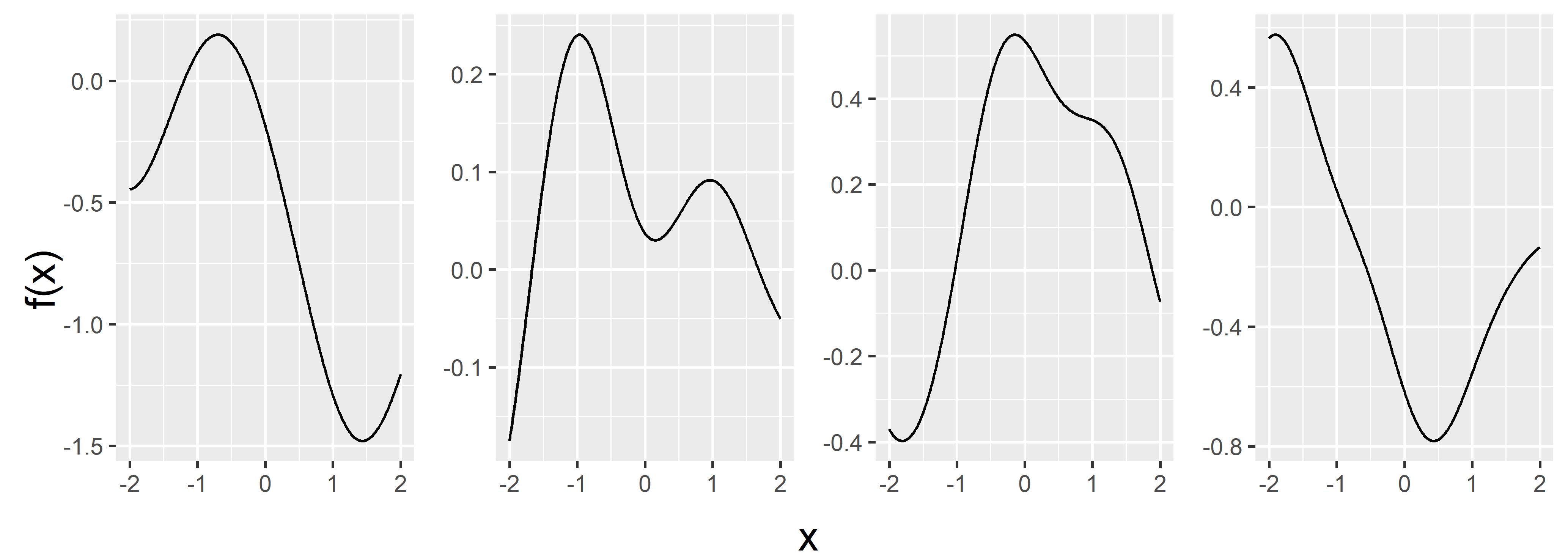
Refer to caption
Figure 10: Four causal functions as modeled by the RBF kernel Gaussian Process.
Figure 11: Boxplot illustrating the SHD performance of CAM and CAT for varying sample sizes, system sizes and tree types in the experiment of Section 6.1.2 with 200 repetitions. CAT.G.cf is the CAT.G method with cross-fitted edge weights. We see that cross-fitting has no positive impact on the performance. It seems to worsen the performance for small sample sizes.
Figure 12: Boxplot illustrating the SID performance of CAM and CAT for varying sample sizes, system sizes and tree types in the experiment of Section 6.1.2. CAT.G is CAT with edge weights derived from the Gaussian score function.
Figure 13: Boxplot illustrating the SHD performance of CAM and CAT for varying sample sizes, system sizes and tree types in the experiment of Section 6.1.2. Here CAT.G is run on the CAM edge weights , so that any difference in nonparametric regression technique is ruled out as the source of the performance difference.
Figure 14: Boxplot of edge relations for the experiment in Section 6.2.
Figure 15: Boxplot of SHD for the experiment in Section 6.2.

Appendix D Proofs

This section contains the proofs of all results presented in the main text.

D.1 Proofs of Section 2

Proof of Lemma 3.Let θ=(𝒢,(fi),PN)∈𝒯p×𝒟3p×𝒫Gp\theta=(\mathcal{G},(f_{i}),P_{N})\in\mathcal{T}_{p}\times\mathcal{D}_{3}^{p}\times\mathcal{P}_{\mathrm{G}}^{p}. Furthermore, let all causal functions (fi)(f_{i}) be nowhere constant and nonlinear. The additive noise is Gaussian, so the log density of NiN_{i} for all i∈{1,…,p}i\in\{1,\ldots,p\} is given by

νi​(x)=−12​log⁡(2​π​σi2)−x22​σi2,νi′​(x)=−xσi2,νi′′​(x)=−1σi2,νi′′′​(x)=0.\displaystyle\nu_{i}(x)=-\frac{1}{2}\log(2\pi\sigma_{i}^{2})-\frac{x^{2}}{2\sigma_{i}^{2}},\quad\nu_{i}^{\prime}(x)=-\frac{x}{\sigma_{i}^{2}},\quad\nu_{i}^{\prime\prime}(x)=-\frac{1}{\sigma_{i}^{2}},\quad\nu_{i}^{\prime\prime\prime}(x)=0.

By assumption we have that condition (i) of Definition 2 is satisfied, hence assume for contradiction that condition (ii) of Definition 2 is not satisfied. That is, we assume that there exists an i∈{1,…,p}∖{rt⁡(𝒢)}i\in\{1,...,p\}\setminus\{\mathrm{rt}(\mathcal{G})\} such that for all

(x,y)∈𝒥:=\displaystyle(x,y)\in\mathcal{J}:= {(x,y)∈ℝ2:νi′′​(y−fi​(x))​fi′​(x)≠0}\displaystyle\,\{(x,y)\in\mathbb{R}^{2}:\nu_{i}^{\prime\prime}(y-f_{i}(x))f^{\prime}_{i}(x)\not=0\}
=\displaystyle= {(x,y)∈ℝ2:fi′​(x)≠0},\displaystyle\,\{(x,y)\in\mathbb{R}^{2}:f_{i}^{\prime}(x)\not=0\},

it holds that

ξ′′′​(x)−ξ′′​(x)​fi′′​(x)fi′​(x)−2​fi′′​(x)​fi′​(x)σ2\displaystyle\xi^{\prime\prime\prime}(x)-\xi^{\prime\prime}(x)\frac{f_{i}^{\prime\prime}(x)}{f_{i}^{\prime}(x)}-\frac{2f_{i}^{\prime\prime}(x)f_{i}^{\prime}(x)}{\sigma^{2}} =−y−fi​(x)σ2​(fi′′′​(x)−(fi′′​(x))2fi′​(x)).\displaystyle=-\frac{y-f_{i}(x)}{\sigma^{2}}\left(f_{i}^{\prime\prime\prime}(x)-\frac{(f_{i}^{\prime\prime}(x))^{2}}{f_{i}^{\prime}(x)}\right). (20)

Henceforth, suppress the subscript ii of fif_{i} and σi\sigma_{i}. First note that {x∈ℝ:f′​(x)=0}\{x\in\mathbb{R}:f^{\prime}(x)=0\} is closed by continuity of f′f^{\prime}. The complement is open, hence there exists a countable collection of mutually disjoint open intervals (Ok)k∈ℤ(O_{k})_{k\in\mathbb{Z}} such that {x∈ℝ:f′(x)≠0}=∪k∈ℤOk\{x\in\mathbb{R}:f^{\prime}(x)\not=0\}=\cup_{k\in\mathbb{Z}}O_{k}. Since ff is nowhere constant we know that {x∈ℝ:f′​(x)=0}\{x\in\mathbb{R}:f^{\prime}(x)=0\} has empty interior which implies that ∪k∈ℤOk¯=ℝ\overline{\cup_{k\in\mathbb{Z}}O_{k}}=\mathbb{R}. Now let (Ok)k∈ℤ(O_{k})_{k\in\mathbb{Z}} be indexed by ℤ\mathbb{Z} such that for any k,j∈ℤk,j\in\mathbb{Z} with k<jk<j and x∈Ok,y∈Ojx\in O_{k},y\in O_{j} it holds that x<yx<y. As the left-hand side of Equation 20 is constant in yy it must hold that

0=f′′′​(x)−(f′′​(x))2f′​(x)=∂f′′​(x)∂x​f′​(x)−f′′​(x)​∂f′​(x)∂x(f′​(x))2=∂∂x​(f′′​(x)f′​(x)),\displaystyle 0=f^{\prime\prime\prime}(x)-\frac{(f^{\prime\prime}(x))^{2}}{f^{\prime}(x)}=\frac{\frac{\partial f^{\prime\prime}(x)}{\partial x}f^{\prime}(x)-f^{\prime\prime}(x)\frac{\partial f^{\prime}(x)}{\partial x}}{(f^{\prime}(x))^{2}}=\frac{\partial}{\partial x}\left(\frac{f^{\prime\prime}(x)}{f^{\prime}(x)}\right),

i.e., f′′​(x)/f′​(x)f^{\prime\prime}(x)/f^{\prime}(x) is constant, for all x∈∪k∈ℤOkx\in\cup_{k\in\mathbb{Z}}O_{k}.

On each OkO_{k} we have that

∂/∂x​log⁡(sign​(f′​(x))​f′​(x))\displaystyle\partial/\partial x\log(\text{sign}(f^{\prime}(x))f^{\prime}(x)) =ck,1⇔\displaystyle=c_{k,1}\iff
log⁡(sign​(f′​(x))​f′​(x))\displaystyle\log(\text{sign}(f^{\prime}(x))f^{\prime}(x)) =ck,1​x+ck,2⇔\displaystyle=c_{k,1}x+c_{k,2}\iff
sign​(f′​(x))​f′​(x)\displaystyle\text{sign}(f^{\prime}(x))f^{\prime}(x) =exp⁡(ck,1​x+ck,2)⇔\displaystyle=\exp(c_{k,1}x+c_{k,2})\iff
f′​(x)\displaystyle f^{\prime}(x) =±exp⁡(ck,1​x+ck,2).\displaystyle=\pm\exp(c_{k,1}x+c_{k,2}).

Recall that we have assumed continuous differentiability of f′f^{\prime}. That is, for any k∈ℤk\in\mathbb{Z} and tk:=sup(Ok)=inf(Ok+1)t_{k}:=\sup(O_{k})=\inf(O_{k+1}) we have limx↑tkf′​(x)=limx↓tkf′​(x)\lim_{x\uparrow t_{k}}f^{\prime}(x)=\lim_{x\downarrow t_{k}}f^{\prime}(x) and limx↑tkf′′​(x)=limx↓tkf′′​(x)\lim_{x\uparrow t_{k}}f^{\prime\prime}(x)=\lim_{x\downarrow t_{k}}f^{\prime\prime}(x). Assume without loss of generality that f′​(x)=exp⁡(ck,1​x+ck,2)f^{\prime}(x)=\exp(c_{k,1}x+c_{k,2}) for all x∈Okx\in O_{k} and k∈ℤk\in\mathbb{Z}. These conditions impose the restrictions (ck,1−ck+1,1)​tk=ck+1,2−ck,2(c_{k,1}-c_{{k+1},1})t_{k}=c_{{k+1},2}-c_{k,2} and log⁡(ck,1/ck+1,1)+(ck,1−ck+1,1)​tk=ck+1,2−ck,2\log(c_{k,1}/c_{k+1,1})+(c_{k,1}-c_{k+1,1})t_{k}=c_{k+1,2}-c_{k,2} which entails that ck,1=ck+1,1c_{k,1}=c_{k+1,1} and ck,2=ck+1,2c_{k,2}=c_{k+1,2}. This proves that there exists c1,c2∈ℝc_{1},c_{2}\in\mathbb{R} such that f′​(x)=exp⁡(c1​x+c2)f^{\prime}(x)=\exp(c_{1}x+c_{2}) for all x∈ℝx\in\mathbb{R}. Thus, the differential equation holds for all x∈ℝx\in\mathbb{R},

0=ξ′′′​(x)−ξ′′​(x)​f′′​(x)f′​(x)−2​f′′​(x)​f′​(x)σ2=∂∂x​(ξ′′​(x)f′​(x))−2​f′′​(x)σ2,\displaystyle 0=\xi^{\prime\prime\prime}(x)-\xi^{\prime\prime}(x)\frac{f^{\prime\prime}(x)}{f^{\prime}(x)}-\frac{2f^{\prime\prime}(x)f^{\prime}(x)}{\sigma^{2}}=\frac{\partial}{\partial x}\left(\frac{\xi^{\prime\prime}(x)}{f^{\prime}(x)}\right)-2\frac{f^{\prime\prime}(x)}{\sigma^{2}},

by division with f′​(x)f^{\prime}(x). By integration this implies that 0=ξ′′​(x)/f′​(x)−2​f′​(x)/σ2+c30=\xi^{\prime\prime}(x)/f^{\prime}(x)-2f^{\prime}(x)/\sigma^{2}+c_{3} such that ξ′′​(x)=2​exp⁡(2​c1​x+2​c2)/σ2−c3​exp⁡(c1​x+c2)\xi^{\prime\prime}(x)=2\exp(2c_{1}x+2c_{2})/\sigma^{2}-c_{3}\exp(c_{1}x+c_{2}) and ξ′​(x)=exp⁡(2​c1​x+2​c2)/c1​σ2−c3​exp⁡(c1​x+c2)/c1+c4\xi^{\prime}(x)=\exp(2c_{1}x+2c_{2})/c_{1}\sigma^{2}-c_{3}\exp(c_{1}x+c_{2})/c_{1}+c_{4} and

ξ⁡(x)=exp⁡(2​c1​x+2​c2)2​c12​σ2−c3​exp⁡(c1​x+c2)c12+c4​x+c5.\displaystyle\xi(x)=\frac{\exp(2c_{1}x+2c_{2})}{2c_{1}^{2}\sigma^{2}}-\frac{c_{3}\exp(c_{1}x+c_{2})}{c_{1}^{2}}+c_{4}x+c_{5}.

We see that ξ⁡(x)→∞⇔pXpa𝒢​(i)​(x)→∞\xi(x)\to\infty\iff p_{X_{{\mathrm{pa}^{\mathcal{G}}({i})}}}(x)\to\infty as x→sign​(c1)⋅∞x\to\text{sign}(c_{1})\cdot\infty, in contradiction with the assumption that pXpa𝒢​(i)​(x)p_{X_{{\mathrm{pa}^{\mathcal{G}}({i})}}}(x) is a probability density function if c1≠0c_{1}\not=0. Thus, it must hold that f′′​(x)/f′​(x)=0f^{\prime\prime}(x)/f^{\prime}(x)=0 for all x∈ℝx\in\mathbb{R}, or equivalently, that ff is a linear function, yielding a contradiction.

This proves that whenever fi∈𝒟3f_{i}\in\mathcal{D}_{3} is a nowhere constant and nonlinear function and the additive noise is Gaussian then condition (ii) of Definition 2 is satisfied, so θ∈ΘR\theta\in\Theta_{R}. ∎

Proof of Proposition 4.First, we consider the bivariate setting. Let (X,Y)(X,Y) be generated by an additive noise SCM θ∈ΘR⊂𝒯2×𝒟32×𝒫𝒞32\theta\in\Theta_{R}\subset\mathcal{T}_{2}\times\mathcal{D}_{3}^{2}\times\mathcal{P}_{\mathcal{C}_{3}}^{2} given by X:=NXX:=N_{X} and Y:=f⁡(X)+NYY:=f(X)+N_{Y} with PX=pX⋅λP_{X}=p_{X}\cdot\lambda and PNY=pNY⋅λP_{N_{Y}}=p_{N_{Y}}\cdot\lambda having three times differentiable strictly positive densities and ff is a three times differentiable nowhere constant function such that condition (ii) of Definition 2 holds.

Assume for contradiction that we do not have observational identifiability of the causal structure 𝒢=(V={X,Y},ℰ={(X→Y)})\mathcal{G}=(V=\{X,Y\},\mathcal{E}=\{(X\to Y)\}). That is, there exists θ~∈𝒯2×𝒟1p×𝒫𝒞0p\tilde{\theta}\in\mathcal{T}_{2}\times\mathcal{D}_{1}^{p}\times\mathcal{P}_{\mathcal{C}_{0}}^{p} with causal graph 𝒢~≠𝒢\tilde{\mathcal{G}}\not=\mathcal{G} or, equivalently, a differentiable function gg and noise distributions PN~X=pN~X⋅λP_{\tilde{N}_{X}}=p_{\tilde{N}_{X}}\cdot\lambda and PN~Y=pN~Y⋅λP_{\tilde{N}_{Y}}=p_{\tilde{N}_{Y}}\cdot\lambda with continuous densities such that the structural assignments Y~:=N~Y\tilde{Y}:=\tilde{N}_{Y} and X~:=g⁡(Y~)+N~X\tilde{X}:=g(\tilde{Y})+\tilde{N}_{X} induce the same distribution, i.e.,

PX,Y=PX~,Y~.\displaystyle P_{X,Y}=P_{\tilde{X},\tilde{Y}}. (21)

By the additive noise structural assignments we know that both PX,YP_{X,Y} and PX~,Y~P_{\tilde{X},\tilde{Y}} have densities with respect to λ2\lambda^{2} given by

pX,Y​(x,y)\displaystyle p_{X,Y}(x,y) =pX​(x)​pNY​(y−f⁡(x)),\displaystyle=p_{X}(x)p_{N_{Y}}(y-f(x)),
pX~,Y~​(x,y)\displaystyle p_{\tilde{X},\tilde{Y}}(x,y) =pN~X​(x−g⁡(y))​pY~​(y),\displaystyle=p_{\tilde{N}_{X}}(x-g(y))p_{\tilde{Y}}(y),

for all (x,y)∈ℝ2(x,y)\in\mathbb{R}^{2}. By the equality of distributions in Equation 21 and strict positivity of pXp_{X} and pNYp_{N_{Y}} we especially have that for λ2\lambda^{2}-almost all (x,y)∈ℝ2(x,y)\in\mathbb{R}^{2}

0<pX,Y​(x,y)=pX~,Y~​(x,y).\displaystyle 0<p_{X,Y}(x,y)=p_{\tilde{X},\tilde{Y}}(x,y). (22)

However, as both pX,Yp_{X,Y} and pX~,Y~p_{\tilde{X},\tilde{Y}} are continuous we realize that the inequality in Equation 22 holds for all (x,y)∈ℝ(x,y)\in\mathbb{R} (if they were not everywhere equal there would exists a non-empty open ball in ℝ2\mathbb{R}^{2} on which they differ in contradiction with λ2\lambda^{2}-almost everywhere equality). Furthermore, by the assumption that ff is three times differentiable and pXp_{X}, pNYp_{N_{Y}} are three times continuously differentiable we have that ∂3π/∂x3\partial^{3}\pi/\partial x^{3} and ∂3π/∂x2​∂y\partial^{3}\pi/\partial x^{2}\partial y are well-defined partial-derivatives of

π⁡(x,y):=log⁡pX,Y​(x,y)=log⁡pX​(x)+log⁡pNY​(y−f⁡(x))=:ξ⁡(x)+ν⁡(y−f⁡(x)),\displaystyle\pi(x,y):=\log p_{X,Y}(x,y)=\log p_{X}(x)+\log p_{N_{Y}}(y-f(x))=:\xi(x)+\nu(y-f(x)),

With π~​(x,y):=log⁡pX~,Y~\tilde{\pi}(x,y):=\log p_{\tilde{X},\tilde{Y}} we have that

π~​(x,y)=log⁡pN~X​(x−g⁡(y))+log⁡pY~​(y)=:ξ~​(x−g⁡(y))+ν~​(y).\displaystyle\tilde{\pi}(x,y)=\log p_{\tilde{N}_{X}}(x-g(y))+\log p_{\tilde{Y}}(y)=:\tilde{\xi}(x-g(y))+\tilde{\nu}(y).

Since it holds that π=π~\pi=\tilde{\pi} by Equation 22 the partial-derivatives ∂3π~/∂x3\partial^{3}\tilde{\pi}/\partial x^{3} and ∂3π~/∂x2​∂y\partial^{3}\tilde{\pi}/\partial x^{2}\partial y are also well-defined. Now note that for any x,y∈ℝx,y\in\mathbb{R}

0=limh→0|π~​(x+h,y)−π~​(x,y)|/h=limh→0|ξ~​(x−g⁡(y)+h)−ξ~​(x−g⁡(y))|/h,\displaystyle 0=\lim_{h\to 0}|\tilde{\pi}(x+h,y)-\tilde{\pi}(x,y)|/h=\lim_{h\to 0}|\tilde{\xi}(x-g(y)+h)-\tilde{\xi}(x-g(y))|/h,

implying that ξ~\tilde{\xi} is differentiable in x−g⁡(y)x-g(y) for any x,y∈ℝx,y\in\mathbb{R} or, equivalently, ξ~\tilde{\xi} is everywhere differentiable. Similar arguments yield that ξ~\tilde{\xi} is at least three times differentiable. We conclude that ∂2π~​(x,y)/∂x2=ξ~′′​(x−g⁡(y))\partial^{2}\tilde{\pi}(x,y)/\partial x^{2}=\tilde{\xi}^{\prime\prime}(x-g(y)) and ∂2π~​(x,y)/∂x​∂y=−ξ~′′​(x−g⁡(y))​g′​(y)\partial^{2}\tilde{\pi}(x,y)/\partial x\partial y=-\tilde{\xi}^{\prime\prime}(x-g(y))g^{\prime}(y) and for any (x,y)∈ℝ2(x,y)\in\mathbb{R}^{2} such that ∂2π~​(x,y)/∂x​∂y≠0\partial^{2}\tilde{\pi}(x,y)/\partial x\partial y\not=0 or, equivalently,

∀(x,y)∈𝒥:={(x,y):∂2π⁡(x,y)∂x​∂y=−ν′′​(y−f⁡(x))​f′​(x)≠0},\forall(x,y)\in\mathcal{J}:=\left\{(x,y):\frac{\partial^{2}\pi(x,y)}{\partial x\partial y}=-\nu^{\prime\prime}(y-f(x))f^{\prime}(x)\not=0\right\},

it holds that

∂∂x​(∂2∂x2​π~​(x,y)∂2∂x​∂y​π~​(x,y))=∂∂x​(−1g′​(y))=0.\displaystyle\frac{\partial}{\partial x}\left(\frac{\frac{\partial^{2}}{\partial x^{2}}\tilde{\pi}(x,y)}{\frac{\partial^{2}}{\partial x\partial y}\tilde{\pi}(x,y)}\right)=\frac{\partial}{\partial x}\left(\frac{-1}{g^{\prime}(y)}\right)=0.

It is worth noting that 𝒥≠∅\mathcal{J}\not=\emptyset to ensure that the following derivations are not void of meaning. (This can be seen by noting that ff is nowhere constant, i.e., f′​(x)≠0f^{\prime}(x)\not=0 for λ\lambda-almost all x∈ℝx\in\mathbb{R}. Hence, 𝒥=∅\mathcal{J}=\emptyset if and only if pNYp_{N_{Y}} is a density such that {(x,y)∈ℝ2:f′​(x)≠0}∋(x,y)↦ν′′​(y−f⁡(x))\{(x,y)\in\mathbb{R}^{2}:f^{\prime}(x)\not=0\}\ni(x,y)\mapsto\nu^{\prime\prime}(y-f(x)) is constantly zero or, equivalently, ℝ∋y↦ν′′​(y)\mathbb{R}\ni y\mapsto\nu^{\prime\prime}(y) is constantly zero. This holds if and only if pNYp_{N_{Y}} is either exponentially decreasing or exponentially increasing everywhere, which is a contradiction as no continuously differentiable function integrating to one has this property.) For any (x,y)∈𝒥(x,y)\in\mathcal{J} we also have that

0=∂∂x​(∂2∂x2​π​(x,y)∂2∂x​∂y​π​(x,y))\displaystyle 0=\frac{\partial}{\partial x}\left(\frac{\frac{\partial^{2}}{\partial x^{2}}\pi(x,y)}{\frac{\partial^{2}}{\partial x\partial y}\pi(x,y)}\right) =∂∂x​(ξ′′​(x)+ν′′​(y−f⁡(x))​f′​(x)2−ν′​(y−f⁡(x))​f′′​(x)−ν′′​(y−f⁡(x))​f′​(x))\displaystyle=\frac{\partial}{\partial x}\left(\frac{\xi^{\prime\prime}(x)+\nu^{\prime\prime}(y-f(x))f^{\prime}(x)^{2}-\nu^{\prime}(y-f(x))f^{\prime\prime}(x)}{-\nu^{\prime\prime}(y-f(x))f^{\prime}(x)}\right)
=−2​f′′+ν′​f′′′ν′′​f′−ξ′′′ν′′​f′+ν′′′​ν′​f′′(ν′′)2\displaystyle=-2f^{\prime\prime}+\frac{\nu^{\prime}f^{\prime\prime\prime}}{\nu^{\prime\prime}f^{\prime}}-\frac{\xi^{\prime\prime\prime}}{\nu^{\prime\prime}f^{\prime}}+\frac{\nu^{\prime\prime\prime}\nu^{\prime}f^{\prime\prime}}{(\nu^{\prime\prime})^{2}}
−ν′′′​ξ′′(ν′′)2−(f′′)2​ν′ν′′​(f′)2+f′′​ξ′′ν′′​(f′)2,\displaystyle\quad-\frac{\nu^{\prime\prime\prime}\xi^{\prime\prime}}{(\nu^{\prime\prime})^{2}}-\frac{(f^{\prime\prime})^{2}\nu^{\prime}}{\nu^{\prime\prime}(f^{\prime})^{2}}+\frac{f^{\prime\prime}\xi^{\prime\prime}}{\nu^{\prime\prime}(f^{\prime})^{2}},

which implies that

ξ′′′=ξ′′​(f′′f′−f′​ν′′′ν′′)−2​ν′′​f′′​f′+ν′​f′′′+ν′′′​ν′​f′′​f′ν′′−ν′​(f′′)2f′,\displaystyle\xi^{\prime\prime\prime}=\xi^{\prime\prime}\left(\frac{f^{\prime\prime}}{f^{\prime}}-\frac{f^{\prime}\nu^{\prime\prime\prime}}{\nu^{\prime\prime}}\right)-2\nu^{\prime\prime}f^{\prime\prime}f^{\prime}+\nu^{\prime}f^{\prime\prime\prime}+\frac{\nu^{\prime\prime\prime}\nu^{\prime}f^{\prime\prime}f^{\prime}}{\nu^{\prime\prime}}-\frac{\nu^{\prime}(f^{\prime\prime})^{2}}{f^{\prime}},

in contradiction with the assumption that condition (ii) of Definition 2 holds. We conclude that PX,Y≠PX~,Y~P_{X,Y}\not=P_{\tilde{X},\tilde{Y}}.

Now consider a multivariate restricted causal model θ∈ΘR\theta\in\Theta_{R} over X=(X1,…,XpCLOSEX=(X_{1},\ldots,X_{p}) with causal directed tree graph 𝒢=(V,ℰ)\mathcal{G}=(V,\mathcal{E}). Assume for contradiction that there exists an alternative SCM θ~=(𝒢~,(f~i),PN~)∈𝒯p×𝒟1p×𝒫𝒞0p\tilde{\theta}=(\tilde{\mathcal{G}},(\tilde{f}_{i}),P_{\tilde{N}})\in\mathcal{T}_{p}\times\mathcal{D}_{1}^{p}\times\mathcal{P}_{\mathcal{C}_{0}}^{p} inducing X~=(X~1,…,X~p)\tilde{X}=(\tilde{X}_{1},\ldots,\tilde{X}_{p}) with causal graph 𝒢~=(V,ℰ~)≠𝒢\tilde{\mathcal{G}}=(V,\tilde{\mathcal{E}})\not=\mathcal{G}, such that PX=PX~P_{X}=P_{\tilde{X}}.

Any SCM induced distribution is Markov with respect to the underlying causal graph. As such, we have that PXP_{X} is Markov with respect to both 𝒢\mathcal{G} and 𝒢~\tilde{\mathcal{G}}. Furthermore, since (in θ\theta) the causal functions are non-constant and the noise innovations have strictly positive density, we have, by Proposition 17 of Peters et al. 2014, that PXP_{X} satisfies causal minimality with respect to causal graph 𝒢\mathcal{G} of θ\theta, i.e., it is globally Markov with respect to 𝒢\mathcal{G} but not any proper subgraph of 𝒢\mathcal{G}. If PXP_{X} also satisfies causal minimality with respect to 𝒢~\tilde{\mathcal{G}}, then, by Proposition 29 of Peters et al. 2014, there exist i,j∈Vi,j\in V such that (j→i)∈ℰ(j\to i)\in\mathcal{E} and (i→j)∈ℰ~(i\to j)\in\tilde{\mathcal{E}}.

Assume for contradiction that PXP_{X} does not satisfy causal minimality with respect to 𝒢~\tilde{\mathcal{G}}. By Proposition 4 of Peters et al. 2014, we have that there exists (j′→i′)∈ℰ~(j^{\prime}\to i^{\prime})\in\tilde{\mathcal{E}} such that Xj′⟂⁣⟂Xi′X_{j^{\prime}}\mathchoice{\mathrel{\hbox to0.0pt{$\displaystyle\perp$\hss}\mkern 2.0mu{\displaystyle\perp}}}{\mathrel{\hbox to0.0pt{$\textstyle\perp$\hss}\mkern 2.0mu{\textstyle\perp}}}{\mathrel{\hbox to0.0pt{$\scriptstyle\perp$\hss}\mkern 2.0mu{\scriptstyle\perp}}}{\mathrel{\hbox to0.0pt{$\scriptscriptstyle\perp$\hss}\mkern 2.0mu{\scriptscriptstyle\perp}}}X_{i^{\prime}}. Define A:=nd𝒢~​(j′)∪{j′}A:={\mathrm{nd}^{\tilde{\mathcal{G}}}({j^{\prime}})}\cup\{j^{\prime}\} and B:=de𝒢~​(i′)∪{i′}B:={\mathrm{de}^{\tilde{\mathcal{G}}}({i^{\prime}})}\cup\{i^{\prime}\}. It holds that A⟂⟂𝒢~(B∖{i′})|i′A{\perp\!\!\!\!\perp_{\tilde{\mathcal{G}}}}(B\setminus\{i^{\prime}\})\,|\,i^{\prime}, i.e., AA and B∖{i′}B\setminus\{i^{\prime}\} are d-separated by i′i^{\prime} in the directed tree 𝒢~\tilde{\mathcal{G}}. Since PXP_{X} is Markov with respect 𝒢~\tilde{\mathcal{G}} it holds that XA⟂⁣⟂XB∖{i′}|Xi′X_{A}\mathchoice{\mathrel{\hbox to0.0pt{$\displaystyle\perp$\hss}\mkern 2.0mu{\displaystyle\perp}}}{\mathrel{\hbox to0.0pt{$\textstyle\perp$\hss}\mkern 2.0mu{\textstyle\perp}}}{\mathrel{\hbox to0.0pt{$\scriptstyle\perp$\hss}\mkern 2.0mu{\scriptstyle\perp}}}{\mathrel{\hbox to0.0pt{$\scriptscriptstyle\perp$\hss}\mkern 2.0mu{\scriptscriptstyle\perp}}}X_{B\setminus\{i^{\prime}\}}\,|\,X_{i^{\prime}}, hence XA⟂⁣⟂XB|Xi′X_{A}\mathchoice{\mathrel{\hbox to0.0pt{$\displaystyle\perp$\hss}\mkern 2.0mu{\displaystyle\perp}}}{\mathrel{\hbox to0.0pt{$\textstyle\perp$\hss}\mkern 2.0mu{\textstyle\perp}}}{\mathrel{\hbox to0.0pt{$\scriptstyle\perp$\hss}\mkern 2.0mu{\scriptstyle\perp}}}{\mathrel{\hbox to0.0pt{$\scriptscriptstyle\perp$\hss}\mkern 2.0mu{\scriptscriptstyle\perp}}}X_{B}\,|\,X_{i^{\prime}}. Similarly, it holds that XA⟂⁣⟂XB|Xj′X_{A}\mathchoice{\mathrel{\hbox to0.0pt{$\displaystyle\perp$\hss}\mkern 2.0mu{\displaystyle\perp}}}{\mathrel{\hbox to0.0pt{$\textstyle\perp$\hss}\mkern 2.0mu{\textstyle\perp}}}{\mathrel{\hbox to0.0pt{$\scriptstyle\perp$\hss}\mkern 2.0mu{\scriptstyle\perp}}}{\mathrel{\hbox to0.0pt{$\scriptscriptstyle\perp$\hss}\mkern 2.0mu{\scriptscriptstyle\perp}}}X_{B}\,|\,X_{j^{\prime}} which implies that XA⟂⁣⟂Xi′|Xj′X_{A}\mathchoice{\mathrel{\hbox to0.0pt{$\displaystyle\perp$\hss}\mkern 2.0mu{\displaystyle\perp}}}{\mathrel{\hbox to0.0pt{$\textstyle\perp$\hss}\mkern 2.0mu{\textstyle\perp}}}{\mathrel{\hbox to0.0pt{$\scriptstyle\perp$\hss}\mkern 2.0mu{\scriptstyle\perp}}}{\mathrel{\hbox to0.0pt{$\scriptscriptstyle\perp$\hss}\mkern 2.0mu{\scriptscriptstyle\perp}}}X_{i^{\prime}}\,|\,X_{j^{\prime}}. By applying the contraction property of conditional independence, we get that

XA⟂⁣⟂Xi′|Xj′andXi′⟂⁣⟂Xj′⟹XA⟂⁣⟂Xi′, and\displaystyle X_{A}\,\mathchoice{\mathrel{\hbox to0.0pt{$\displaystyle\perp$\hss}\mkern 2.0mu{\displaystyle\perp}}}{\mathrel{\hbox to0.0pt{$\textstyle\perp$\hss}\mkern 2.0mu{\textstyle\perp}}}{\mathrel{\hbox to0.0pt{$\scriptstyle\perp$\hss}\mkern 2.0mu{\scriptstyle\perp}}}{\mathrel{\hbox to0.0pt{$\scriptscriptstyle\perp$\hss}\mkern 2.0mu{\scriptscriptstyle\perp}}}X_{i^{\prime}}\,|\,X_{j^{\prime}}\quad\text{and}\quad X_{i^{\prime}}\,\mathchoice{\mathrel{\hbox to0.0pt{$\displaystyle\perp$\hss}\mkern 2.0mu{\displaystyle\perp}}}{\mathrel{\hbox to0.0pt{$\textstyle\perp$\hss}\mkern 2.0mu{\textstyle\perp}}}{\mathrel{\hbox to0.0pt{$\scriptstyle\perp$\hss}\mkern 2.0mu{\scriptstyle\perp}}}{\mathrel{\hbox to0.0pt{$\scriptscriptstyle\perp$\hss}\mkern 2.0mu{\scriptscriptstyle\perp}}}X_{j^{\prime}}\implies X_{A}\mathchoice{\mathrel{\hbox to0.0pt{$\displaystyle\perp$\hss}\mkern 2.0mu{\displaystyle\perp}}}{\mathrel{\hbox to0.0pt{$\textstyle\perp$\hss}\mkern 2.0mu{\textstyle\perp}}}{\mathrel{\hbox to0.0pt{$\scriptstyle\perp$\hss}\mkern 2.0mu{\scriptstyle\perp}}}{\mathrel{\hbox to0.0pt{$\scriptscriptstyle\perp$\hss}\mkern 2.0mu{\scriptscriptstyle\perp}}}X_{i^{\prime}},\text{ and }
XA⟂⁣⟂XB|Xi′andXA⟂⁣⟂Xi′⟹XA⟂⁣⟂XB.\displaystyle X_{A}\,\mathchoice{\mathrel{\hbox to0.0pt{$\displaystyle\perp$\hss}\mkern 2.0mu{\displaystyle\perp}}}{\mathrel{\hbox to0.0pt{$\textstyle\perp$\hss}\mkern 2.0mu{\textstyle\perp}}}{\mathrel{\hbox to0.0pt{$\scriptstyle\perp$\hss}\mkern 2.0mu{\scriptstyle\perp}}}{\mathrel{\hbox to0.0pt{$\scriptscriptstyle\perp$\hss}\mkern 2.0mu{\scriptscriptstyle\perp}}}X_{B}\,|\,X_{i^{\prime}}\quad\text{and}\quad X_{A}\,\mathchoice{\mathrel{\hbox to0.0pt{$\displaystyle\perp$\hss}\mkern 2.0mu{\displaystyle\perp}}}{\mathrel{\hbox to0.0pt{$\textstyle\perp$\hss}\mkern 2.0mu{\textstyle\perp}}}{\mathrel{\hbox to0.0pt{$\scriptstyle\perp$\hss}\mkern 2.0mu{\scriptstyle\perp}}}{\mathrel{\hbox to0.0pt{$\scriptscriptstyle\perp$\hss}\mkern 2.0mu{\scriptscriptstyle\perp}}}X_{i^{\prime}}\implies X_{A}\,\mathchoice{\mathrel{\hbox to0.0pt{$\displaystyle\perp$\hss}\mkern 2.0mu{\displaystyle\perp}}}{\mathrel{\hbox to0.0pt{$\textstyle\perp$\hss}\mkern 2.0mu{\textstyle\perp}}}{\mathrel{\hbox to0.0pt{$\scriptstyle\perp$\hss}\mkern 2.0mu{\scriptstyle\perp}}}{\mathrel{\hbox to0.0pt{$\scriptscriptstyle\perp$\hss}\mkern 2.0mu{\scriptscriptstyle\perp}}}X_{B}.

Since A∪B=V,A∩B=∅A\cup B=V,A\cap B=\emptyset and 𝒢\mathcal{G} is a directed tree (that spans VV) there exist either an edge (j′′→i′′)∈ℰ(j^{\prime\prime}\to i^{\prime\prime})\in\mathcal{E} with j′′∈Aj^{\prime\prime}\in A and i′′∈Bi^{\prime\prime}\in B or j′′∈Bj^{\prime\prime}\in B and i′′∈Ai^{\prime\prime}\in A. In either case, we have that Xi′′⟂⁣⟂Xj′′X_{i^{\prime\prime}}\mathchoice{\mathrel{\hbox to0.0pt{$\displaystyle\perp$\hss}\mkern 2.0mu{\displaystyle\perp}}}{\mathrel{\hbox to0.0pt{$\textstyle\perp$\hss}\mkern 2.0mu{\textstyle\perp}}}{\mathrel{\hbox to0.0pt{$\scriptstyle\perp$\hss}\mkern 2.0mu{\scriptstyle\perp}}}{\mathrel{\hbox to0.0pt{$\scriptscriptstyle\perp$\hss}\mkern 2.0mu{\scriptscriptstyle\perp}}}X_{j^{\prime\prime}}, which contradicts PXP_{X} satisfying causal minimality with respect to 𝒢\mathcal{G}. We conclude that PXP_{X} also satisfies causal minimality with respect to the alternative graph 𝒢~\tilde{\mathcal{G}}.

Hence, the following structural equations hold for (Xi,Xj)(X_{i},X_{j}) and (X~i,X~j)(\tilde{X}_{i},\tilde{X}_{j})

Xi\displaystyle X_{i} =fi​(Xj)+Ni,withXj⟂⁣⟂Ni,\displaystyle=f_{i}(X_{j})+N_{i},\quad\text{with}\quad X_{j}\mathchoice{\mathrel{\hbox to0.0pt{$\displaystyle\perp$\hss}\mkern 2.0mu{\displaystyle\perp}}}{\mathrel{\hbox to0.0pt{$\textstyle\perp$\hss}\mkern 2.0mu{\textstyle\perp}}}{\mathrel{\hbox to0.0pt{$\scriptstyle\perp$\hss}\mkern 2.0mu{\scriptstyle\perp}}}{\mathrel{\hbox to0.0pt{$\scriptscriptstyle\perp$\hss}\mkern 2.0mu{\scriptscriptstyle\perp}}}N_{i},
X~j\displaystyle\tilde{X}_{j} =f~j​(X~i)+N~j,withX~i⟂⁣⟂N~j,\displaystyle=\tilde{f}_{j}(\tilde{X}_{i})+\tilde{N}_{j},\quad\text{with}\quad\tilde{X}_{i}\mathchoice{\mathrel{\hbox to0.0pt{$\displaystyle\perp$\hss}\mkern 2.0mu{\displaystyle\perp}}}{\mathrel{\hbox to0.0pt{$\textstyle\perp$\hss}\mkern 2.0mu{\textstyle\perp}}}{\mathrel{\hbox to0.0pt{$\scriptstyle\perp$\hss}\mkern 2.0mu{\scriptstyle\perp}}}{\mathrel{\hbox to0.0pt{$\scriptscriptstyle\perp$\hss}\mkern 2.0mu{\scriptscriptstyle\perp}}}\tilde{N}_{j},

with PXj,Xi=PX~j,X~iP_{X_{j},X_{i}}=P_{\tilde{X}_{j},\tilde{X}_{i}}. We can apply the same arguments as in the bivariate setup if we can argue that a density of XjX_{j} is three times differentiable and that a density of X~i\tilde{X}_{i} is a continuous density.

To this end, note that the density pXjp_{X_{j}} is given by the convolution of two densities

pXj​(y)=∫−∞∞pfj​(Xpa𝒢​(j))​(t)​pNj​(y−t)​𝑑t,\displaystyle p_{X_{j}}(y)=\int_{-\infty}^{\infty}p_{f_{j}(X_{{\mathrm{pa}^{\mathcal{G}}({j})}})}(t)p_{N_{j}}(y-t)\,dt, (23)

as Xj:=fj​(Xpa𝒢​(j))+NjX_{j}:=f_{j}(X_{{\mathrm{pa}^{\mathcal{G}}({j})}})+N_{j} with Xpa𝒢​(j)⟂⁣⟂NjX_{{\mathrm{pa}^{\mathcal{G}}({j})}}\mathchoice{\mathrel{\hbox to0.0pt{$\displaystyle\perp$\hss}\mkern 2.0mu{\displaystyle\perp}}}{\mathrel{\hbox to0.0pt{$\textstyle\perp$\hss}\mkern 2.0mu{\textstyle\perp}}}{\mathrel{\hbox to0.0pt{$\scriptstyle\perp$\hss}\mkern 2.0mu{\scriptstyle\perp}}}{\mathrel{\hbox to0.0pt{$\scriptscriptstyle\perp$\hss}\mkern 2.0mu{\scriptscriptstyle\perp}}}N_{j}. Here we used that fj​(Xpa𝒢​(j))f_{j}(X_{{\mathrm{pa}^{\mathcal{G}}({j})}}) has density with respect to the Lebesgue measure.

To realize this note that fj∈𝒞3f_{j}\in\mathcal{C}_{3} and it is nowhere constant. By arguments similar to those in the proof of Lemma 3, this implies that f′​(x)=0f^{\prime}(x)=0 at only countably many points (dk)(d_{k}). Now let (Ok)(O_{k}) be the countable collection of mutually disjoint open intervals that cover ℝ\mathbb{R} except for the points (dk)(d_{k}). By continuity of f′f^{\prime} we know that f′​(x)f^{\prime}(x) is either strictly positive or strictly negative on each OkO_{k}. That is, ff is continuously differentiable and strictly monotone on each OkO_{k}. Thus, ff has a continuously differentiable inverse on each OkO_{k} by, e.g., the inverse function theorem. This ensures that fj​(Xpa𝒢​(j))f_{j}(X_{{\mathrm{pa}^{\mathcal{G}}({j})}}) has a density with respect to the Lebesgue measure whenever Xpa𝒢​(j)X_{{\mathrm{pa}^{\mathcal{G}}({j})}} does. By starting at the root node Xrt⁡(𝒢)=Nrt⁡(𝒢)X_{\mathrm{rt}(\mathcal{G})}=N_{\mathrm{rt}(\mathcal{G})}, which by assumption has a density, we can iteratively apply the above argumentation down the directed path from rt⁡(𝒢)\mathrm{rt}(\mathcal{G}) to jj in order to conclude that any XjX_{j} for j∈{1,…,p}j\in\{1,\ldots,p\} has a density with respect to the Lebesgue measure.

Since pNjp_{N_{j}} is assumed strictly positive three times continuous differentiable, the representation in Equation 23 furthermore yields that pXjp_{X_{j}} is three times differentiable; see, e.g., Theorem 11.4 and 11.5 of Schilling 2017.

Now we argue that X~i\tilde{X}_{i} has a continuous density. First note that PXiP_{X_{i}} at least has a continuous density pXip_{X_{i}} by arguments similar to those applied for Equation 23. By the assumption that PX=PX~P_{X}=P_{\tilde{X}} we especially have that PXi=PX~iP_{X_{i}}=P_{\tilde{X}_{i}} which implies that also X~i\tilde{X}_{i} has a continuous density. By virtue of the arguments for the bivariate setup we arrive at a contradiction, so it must hold that PX≠PX~P_{X}\not=P_{\tilde{X}}. ∎

Proof of Lemma 6.Consider an SCM θ~=(𝒢~,(f~i),PN~)∈{𝒢~}×𝒟1p×𝒫Gp\tilde{\theta}=(\tilde{\mathcal{G}},(\tilde{f}_{i}),P_{\tilde{N}})\in\{\tilde{\mathcal{G}}\}\times\mathcal{D}_{1}^{p}\times\mathcal{P}_{\mathrm{G}}^{p} with 𝒢~≠𝒢\tilde{\mathcal{G}}\not=\mathcal{G} and let Qθ~Q_{\tilde{\theta}} be the induced distribution. As Qθ~Q_{\tilde{\theta}} is Markov with respect to 𝒢~\tilde{\mathcal{G}} and generated by an additive noise model the density qθ~q_{\tilde{\theta}} factorizes as

qθ~​(x)=∏i=1pqθ~​(xi|xpa𝒢~​(i))=∏i=1pqN~i​(xi−f~i​(xpa𝒢~​(i))).\displaystyle q_{\tilde{\theta}}(x)=\prod_{i=1}^{p}q_{\tilde{\theta}}(x_{i}|x_{{\mathrm{pa}^{\tilde{\mathcal{G}}}({i})}})=\prod_{i=1}^{p}q_{\tilde{N}_{i}}(x_{i}-\tilde{f}_{i}(x_{{\mathrm{pa}^{\tilde{\mathcal{G}}}({i})}})).

The cross entropy between PXP_{X} and Qθ~Q_{\tilde{\theta}} is then given by

h⁡(PX,Qθ~)\displaystyle h(P_{X},Q_{\tilde{\theta}}) :=𝔼⁡[−log⁡(qθ~​(X))]\displaystyle:=\mathbb{E}\left[-\log\left(q_{\tilde{\theta}}(X)\right)\right]
=∑i=1p𝔼⁡[−log⁡(qN~i​(Xi−f~i​(Xpa𝒢~​(i))))]\displaystyle=\sum_{i=1}^{p}\mathbb{E}\left[-\log\left(q_{\tilde{N}_{i}}\left(X_{i}-\tilde{f}_{i}(X_{{\mathrm{pa}^{\tilde{\mathcal{G}}}({i})}})\right)\right)\right]
=∑i=1ph⁡(Xi−f~i​(Xpa𝒢~​(i)),N~i),\displaystyle=\sum_{i=1}^{p}h\left(X_{i}-\tilde{f}_{i}(X_{{\mathrm{pa}^{\tilde{\mathcal{G}}}({i})}}),\tilde{N}_{i}\right),

where the latter is a sum of the cross entropies between the distribution of Xi−f~i​(Xpa𝒢~​(i))X_{i}-\tilde{f}_{i}(X_{{\mathrm{pa}^{\tilde{\mathcal{G}}}({i})}}) and the distribution of N~i\tilde{N}_{i}. As Qθ~Q_{\tilde{\theta}} is generated by a causal additive tree model with Gaussian noise, we have for all 1≤i≤p1\leq i\leq p that N~i∼𝒩⁡(0,σ~i2)\tilde{N}_{i}\sim\mathcal{N}(0,\tilde{\sigma}_{i}^{2}) for some σ~i2>0\tilde{\sigma}_{i}^{2}>0. Hence for all 1≤i≤p1\leq i\leq p,

h⁡(Xi−f~i​(Xpa𝒢~​(i)),N~i)=\displaystyle h\left(X_{i}-\tilde{f}_{i}(X_{{\mathrm{pa}^{\tilde{\mathcal{G}}}({i})}}),\tilde{N}_{i}\right)= 𝔼⁡[−log⁡(12​π​σi​exp⁡(−(Xi−f~i​(Xpa𝒢~​(i)))22​σ~i2))]\displaystyle\,\mathbb{E}\left[-\log\left(\frac{1}{\sqrt{2\pi}\sigma_{i}}\exp\left(-\frac{\left(X_{i}-\tilde{f}_{i}(X_{{\mathrm{pa}^{\tilde{\mathcal{G}}}({i})}})\right)^{2}}{2\tilde{\sigma}_{i}^{2}}\right)\right)\right]
=\displaystyle= log⁡(2​π​σ~i)+𝔼⁡[(Xi−f~i​(Xpa𝒢~​(i)))2]2​σ~i2.\displaystyle\,\log(\sqrt{2\pi}\tilde{\sigma}_{i})+\frac{\mathbb{E}\left[\left(X_{i}-\tilde{f}_{i}(X_{{\mathrm{pa}^{\tilde{\mathcal{G}}}({i})}})\right)^{2}\right]}{2\tilde{\sigma}_{i}^{2}}.

Thus, for given set of causal functions (f~i)(\tilde{f}_{i}) and a fixed ii, the noise variance that minimizes the cross entropy is given by

σ~i=𝔼⁡[(Xi−f~i​(Xpa𝒢~​(i)))2].\displaystyle\tilde{\sigma}_{i}=\sqrt{\mathbb{E}\left[\left(X_{i}-\tilde{f}_{i}(X_{{\mathrm{pa}^{\tilde{\mathcal{G}}}({i})}})\right)^{2}\right]}.

We thus have

infσ~i>0{log⁡(2​π​σ~i)+𝔼⁡[(Xi−f~i​(Xpa𝒢~​(i)))2]2​σ~i2}\displaystyle\inf_{\tilde{\sigma}_{i}>0}\left\{\log(\sqrt{2\pi}\tilde{\sigma}_{i})+\frac{\mathbb{E}\left[\left(X_{i}-\tilde{f}_{i}(X_{{\mathrm{pa}^{\tilde{\mathcal{G}}}({i})}})\right)^{2}\right]}{2\tilde{\sigma}_{i}^{2}}\right\}
=log⁡(2​π)+12​log⁡(𝔼⁡[(Xi−f~i​(Xpa𝒢~​(i)))2])+12.\displaystyle=\,\log\left(\sqrt{2\pi}\right)+\frac{1}{2}\log\left(\mathbb{E}\left[\left(X_{i}-\tilde{f}_{i}(X_{{\mathrm{pa}^{\tilde{\mathcal{G}}}({i})}})\right)^{2}\right]\right)+\frac{1}{2}.

We conclude that

infQ∈{𝒢~}×𝒟1p×𝒫Gph⁡(PX,Q)\displaystyle\,\inf_{Q\in\{\tilde{\mathcal{G}}\}\times\mathcal{D}_{1}^{p}\times\mathcal{P}_{\mathrm{G}}^{p}}h(P_{X},Q)
=\displaystyle= p​log⁡(2​π)+p2+∑i=1p12​log⁡(inff~i∈𝒟1𝔼⁡[(Xi−f~i​(Xpa𝒢~​(i)))2]).\displaystyle\,p\log(\sqrt{2\pi})+\frac{p}{2}+\sum_{i=1}^{p}\frac{1}{2}\log\left(\inf_{\tilde{f}_{i}\in\mathcal{D}_{1}}\mathbb{E}\left[\left(X_{i}-\tilde{f}_{i}(X_{{\mathrm{pa}^{\tilde{\mathcal{G}}}({i})}})\right)^{2}\right]\right).

Finally, as 𝒟1\mathcal{D}_{1} is dense in ℒ2​(PXpa𝒢~​(i))\mathcal{L}^{2}(P_{X_{{\mathrm{pa}^{\tilde{\mathcal{G}}}({i})}}}), we have that

inff~i∈𝒟1𝔼⁡[(Xi−f~i​(Xpa𝒢~​(i)))2]\displaystyle\inf_{\tilde{f}_{i}\in\mathcal{D}_{1}}\mathbb{E}\left[\left(X_{i}-\tilde{f}_{i}(X_{{\mathrm{pa}^{\tilde{\mathcal{G}}}({i})}})\right)^{2}\right] =𝔼[(Xi−𝔼[Xi|Xpa𝒢~​(i)]))2]\displaystyle=\mathbb{E}\left[\left(X_{i}-\mathbb{E}[X_{i}|X_{{\mathrm{pa}^{\tilde{\mathcal{G}}}({i})}}])\right)^{2}\right]
+inff~i∈𝒟1𝔼[(𝔼[Xi|Xpa𝒢~​(i)]−f~i(Xpa𝒢~​(i)))2]\displaystyle\quad+\inf_{\tilde{f}_{i}\in\mathcal{D}_{1}}\mathbb{E}\left[\left(\mathbb{E}[X_{i}|X_{{\mathrm{pa}^{\tilde{\mathcal{G}}}({i})}}]-\tilde{f}_{i}(X_{{\mathrm{pa}^{\tilde{\mathcal{G}}}({i})}})\right)^{2}\right]
=𝔼[(Xi−𝔼[Xi|Xpa𝒢~​(i)]))2].\displaystyle=\mathbb{E}\left[\left(X_{i}-\mathbb{E}[X_{i}|X_{{\mathrm{pa}^{\tilde{\mathcal{G}}}({i})}}])\right)^{2}\right].

Here we used that Xpa𝒢~​(i)X_{{\mathrm{pa}^{\tilde{\mathcal{G}}}({i})}} has density with respect to the Lebesgue measure, PXpa𝒢~​(i)≪λP_{X_{{\mathrm{pa}^{\tilde{\mathcal{G}}}({i})}}}\ll\lambda, and that the density is differentiable (see proof of Proposition 4). This concludes the first part of the proof.

For the second statement, we note that for any Q∈{𝒢~}×ℱ⁡(𝒢~)×𝒫pQ\in\{\tilde{\mathcal{G}}\}\times\mathcal{F}(\tilde{\mathcal{G}})\times\mathcal{P}^{p} there exists some noise innovation distribution PN~∈𝒫P_{\tilde{N}}\in\ \mathcal{P} such that QQ is the distribution of X~\tilde{X} generated by structural assignments

X~i:=f~i​(Xpa𝒢~​(i))+N~i=𝔼⁡[Xi|Xpa𝒢~​(i)]+N~i,\displaystyle\tilde{X}_{i}:=\tilde{f}_{i}(X_{{\mathrm{pa}^{\tilde{\mathcal{G}}}({i})}})+\tilde{N}_{i}=\mathbb{E}[X_{i}|X_{{\mathrm{pa}^{\tilde{\mathcal{G}}}({i})}}]+\tilde{N}_{i},

for all 1≤j≤p1\leq j\leq p and mutually independent noise innovations N~=(N~1,…,N~p)∼PN~∈𝒫p\tilde{N}=(\tilde{N}_{1},\ldots,\tilde{N}_{p})\sim P_{\tilde{N}}\in\mathcal{P}^{p}. Let qq denote the density of QQ with respect to the Lebesgue measure and let qN~iq_{\tilde{N}_{i}} denote the density of N~i\tilde{N}_{i} for all 1≤i≤p1\leq i\leq p. As QQ is Markov with respect to 𝒢~\tilde{\mathcal{G}} and generated by an additive noise model the density factorizes as

q⁡(x)=∏i=1pq⁡(xi|xpa𝒢~​(i))=∏i=1pqN~i​(xi−𝔼⁡[Xi|Xpa𝒢~​(i)=xpa𝒢~​(i)]).\displaystyle q(x)=\prod_{i=1}^{p}q(x_{i}|x_{{\mathrm{pa}^{\tilde{\mathcal{G}}}({i})}})=\prod_{i=1}^{p}q_{\tilde{N}_{i}}(x_{i}-\mathbb{E}[X_{i}|X_{{\mathrm{pa}^{\tilde{\mathcal{G}}}({i})}}=x_{{\mathrm{pa}^{\tilde{\mathcal{G}}}({i})}}]).

The cross entropy between PXP_{X} and QQ is given by

h⁡(PX,Q)\displaystyle h(P_{X},Q) =𝔼⁡[−log⁡(q⁡(X))]\displaystyle=\mathbb{E}\left[-\log\left(q(X)\right)\right]
=∑i=1p𝔼⁡[−log⁡(q⁡(Xi|Xpa𝒢~​(i)))]\displaystyle=\sum_{i=1}^{p}\mathbb{E}\left[-\log\left(q(X_{i}|X_{{\mathrm{pa}^{\tilde{\mathcal{G}}}({i})}})\right)\right]
=∑i=1p𝔼⁡[−log⁡(qN~i​(Xi−𝔼⁡[Xi|Xpa𝒢~​(i)]))]\displaystyle=\sum_{i=1}^{p}\mathbb{E}\left[-\log\left(q_{\tilde{N}_{i}}\left(X_{i}-\mathbb{E}\left[X_{i}|X_{{\mathrm{pa}^{\tilde{\mathcal{G}}}({i})}}\right]\right)\right)\right]
=∑i=1ph⁡(Xi−𝔼⁡[Xi|Xpa𝒢~​(i)],N~i).\displaystyle=\sum_{i=1}^{p}h\left(X_{i}-\mathbb{E}\left[X_{i}|X_{{\mathrm{pa}^{\tilde{\mathcal{G}}}({i})}}\right],\tilde{N}_{i}\right).

Note that h(P,Q)=h(P)+DKL(P∥Q)≥h(P)h(P,Q)=h(P)+D_{\mathrm{KL}}(P\|Q)\geq h(P) with equality if and only if Q=PQ=P. Thus, the infimum is attained at noise innovations that are equal in distribution to Xi−𝔼⁡[Xi|Xpa𝒢~​(i)]X_{i}-\mathbb{E}[X_{i}|X_{{\mathrm{pa}^{\tilde{\mathcal{G}}}({i})}}] (which has a density by assumption). That is,

infQ∈{𝒢~}×ℱ⁡(𝒢~)×𝒫ph⁡(PX,Q)\displaystyle\inf_{Q\in\{\tilde{\mathcal{G}}\}\times\mathcal{F}(\tilde{\mathcal{G}})\times\mathcal{P}^{p}}h(P_{X},Q) =∑i=1pinfN~j∼PN~j∈𝒫h⁡(Xi−𝔼⁡[Xi|Xpa𝒢~​(i)],N~i)\displaystyle=\sum_{i=1}^{p}\inf_{\tilde{N}_{j}\sim P_{\tilde{N}_{j}}\in\mathcal{P}}h\left(X_{i}-\mathbb{E}\left[X_{i}|X_{{\mathrm{pa}^{\tilde{\mathcal{G}}}({i})}}\right],\tilde{N}_{i}\right)
=∑i=1ph⁡(Xi−𝔼⁡[Xi|Xpa𝒢~​(i)])\displaystyle=\sum_{i=1}^{p}h\left(X_{i}-\mathbb{E}\left[X_{i}|X_{{\mathrm{pa}^{\tilde{\mathcal{G}}}({i})}}\right]\right)
=ℓE​(𝒢~).\displaystyle=\ell_{\mathrm{E}}(\tilde{\mathcal{G}}).

∎

Proof of Lemma 7.Let θ∈ΘR⊂𝒯p×𝒟3p×𝒫Gp\theta\in\Theta_{R}\subset\mathcal{T}_{p}\times\mathcal{D}_{3}^{p}\times\mathcal{P}_{\mathrm{G}}^{p} and assume that condition (a) is satisfied, i.e., that for all i≠ji\not=j it holds that x↦𝔼⁡[Xi|Xj=x]x\mapsto\mathbb{E}[X_{i}|X_{j}=x] has a differentiable version. Note that

ℓG​(𝒢~)−ℓG​(𝒢)=infQ∈{𝒢~}×𝒟1p×𝒫Gph⁡(PX,Q)−h⁡(PX).\displaystyle\ell_{\mathrm{G}}(\tilde{\mathcal{G}})-\ell_{\mathrm{G}}(\mathcal{G})=\inf_{Q\in\{\tilde{\mathcal{G}}\}\times\mathcal{D}_{1}^{p}\times\mathcal{P}_{\mathrm{G}}^{p}}h(P_{X},Q)-h(P_{X}). (24)

Furthermore, by the considerations in the proof of Lemma 6 the infimum in Equation 24 is attained for Q∗Q^{*}, where the functions are given by the conditional expectation functionals. When condition (a) is satisfied we therefore know that Q∗∈{𝒢~}×𝒟1p×𝒫GpQ^{*}\in\{\tilde{\mathcal{G}}\}\times\mathcal{D}_{1}^{p}\times\mathcal{P}_{\mathrm{G}}^{p}. Finally,

ℓG(𝒢~)−ℓG(𝒢)=h(PX,Q∗)−h(PX)=DKL(PX∥Q∗)>0,\displaystyle\ell_{\mathrm{G}}(\tilde{\mathcal{G}})-\ell_{\mathrm{G}}(\mathcal{G})=h(P_{X},Q^{*})-h(P_{X})=D_{\mathrm{KL}}(P_{X}\,\|\,Q^{*})>0,

where the last strict inequality follows from Proposition 4.

Now let θ∈ΘR⊂𝒯p×𝒟3p×𝒫Gp\theta\in\Theta_{R}\subset\mathcal{T}_{p}\times\mathcal{D}_{3}^{p}\times\mathcal{P}_{\mathrm{G}}^{p}. Assume that condition (b) is satisfied, i.e., for all 1≤i≤p1\leq i\leq p it holds that the causal function fif_{i} is contained within a function class ℱi⊆𝒟1\mathcal{F}_{i}\subseteq\mathcal{D}_{1}, which for all j≠ij\not=i satisfies

arg​minf~i∈ℱi⁡𝔼​[(Xi−f~i​(Xj))2]∈ℱi.\displaystyle\argmin_{\tilde{f}_{i}\in\mathcal{F}_{i}}\mathbb{E}\left[\left(X_{i}-\tilde{f}_{i}(X_{j})\right)^{2}\right]\in\mathcal{F}_{i}. (25)

Define the modified Gaussian score function

ℓG.mod​(𝒢~):=∑i=1p12​log⁡(Var⁡(Xi−fpa𝒢~​(i)​i​(Xpa𝒢~​(i)))),\displaystyle\ell_{\mathrm{G.mod}}(\tilde{\mathcal{G}}):=\sum_{i=1}^{p}\frac{1}{2}\log\left(\mathrm{Var}\left(X_{i}-f_{{\mathrm{pa}^{\tilde{\mathcal{G}}}({i})}i}(X_{{\mathrm{pa}^{\tilde{\mathcal{G}}}({i})}})\right)\right),

where fj​i:ℝ→ℝf_{ji}:\mathbb{R}\to\mathbb{R} is given by

fj​i:=arg​minf~∈ℱi⁡𝔼​[(Xi−f~​(Xj))2],\displaystyle f_{ji}:=\argmin_{\tilde{f}\in\mathcal{F}_{i}}\mathbb{E}\left[\left(X_{i}-\tilde{f}(X_{j})\right)^{2}\right],

for all i≠ji\not=j. Now, for any 𝒢~∈𝒯p∖{𝒢}\tilde{\mathcal{G}}\in\mathcal{T}_{p}\setminus\{\mathcal{G}\}, it holds that

ℓG.mod​(𝒢~)−ℓG.mod​(𝒢)\displaystyle\ell_{\mathrm{G.mod}}(\tilde{\mathcal{G}})-\ell_{\mathrm{G.mod}}(\mathcal{G}) =infQ∈{𝒢~}×(ℱi)1≤i≤p×𝒫Gph⁡(PX,Q)−h⁡(PX)\displaystyle=\inf_{Q\in\{\tilde{\mathcal{G}}\}\times(\mathcal{F}_{i})_{1\leq i\leq p}\times\mathcal{P}_{\mathrm{G}}^{p}}h(P_{X},Q)-h(P_{X})
=h⁡(PX,Q∗)−h⁡(PX)\displaystyle=h(P_{X},Q^{*})-h(P_{X})
=DKL(PX∥Q∗)>0.\displaystyle=D_{\mathrm{KL}}(P_{X}\,\|\,Q^{*})>0.

Here we used the closedness in Equation 25 to argue that the infimum is attained for Q∗∈{𝒢~}×(ℱi)1≤i≤p×𝒫GpQ^{*}\in\{\tilde{\mathcal{G}}\}\times(\mathcal{F}_{i})_{1\leq i\leq p}\times\mathcal{P}_{\mathrm{G}}^{p}. Finally, since (ℱi)1≤i≤p⊂𝒟1p(\mathcal{F}_{i})_{1\leq i\leq p}\subset\mathcal{D}_{1}^{p}, Proposition 4 guarantees the strict inequality.

Now let θ∈ΘR⊂𝒯p×𝒟3p×𝒫+𝒞3p\theta\in\Theta_{R}\subset\mathcal{T}_{p}\times\mathcal{D}_{3}^{p}\times\mathcal{P}_{+\mathcal{C}_{3}}^{p}. Assume that for all i≠ji\not=j it holds that x↦𝔼⁡[Xi|Xj=x]x\mapsto\mathbb{E}[X_{i}|X_{j}=x] has a differentiable version, and assume that for all i≠ji\not=j it holds that Xi−𝔼⁡[Xi|Xj]X_{i}-\mathbb{E}[X_{i}|X_{j}] has a continuous density. With these assumptions we note that for any 𝒢~∈𝒯p∖{𝒢}\tilde{\mathcal{G}}\in\mathcal{T}_{p}\setminus\{\mathcal{G}\} it holds, by the arguments in the proof of Lemma 6, that

ℓE​(𝒢~)−ℓE​(𝒢)=infQ∈{𝒢~}×ℱ⁡(𝒢~)×𝒫ph⁡(PX,Q)−h⁡(PX)=h⁡(PX,Q∗)−h⁡(PX),\displaystyle\ell_{\mathrm{E}}(\tilde{\mathcal{G}})-\ell_{\mathrm{E}}(\mathcal{G})=\inf_{Q\in\{\tilde{\mathcal{G}}\}\times\mathcal{F}(\tilde{\mathcal{G}})\times\mathcal{P}^{p}}h(P_{X},Q)-h(P_{X})=h(P_{X},Q^{*})-h(P_{X}),

where Q∗Q^{*} is generated by an additive noise model 𝒢~×(fi)×(PN~i)1≤i≤p\tilde{\mathcal{G}}\times(f_{i})\times(P_{\tilde{N}_{i}})_{1\leq i\leq p} with causal graph 𝒢~∈𝒯p\tilde{\mathcal{G}}\in\mathcal{T}_{p}, with causal functions fi≡x↦𝔼⁡[Xi|Xpa𝒢~​(i)=x]∈𝒟1f_{i}\equiv x\mapsto\mathbb{E}[X_{i}|X_{{\mathrm{pa}^{\tilde{\mathcal{G}}}({i})}}=x]\in\mathcal{D}_{1} and noise innovations given by N~i=𝒟Xi−𝔼⁡[Xi|Xj]∼PNi∈𝒫𝒞0\tilde{N}_{i}\stackrel{{\scriptstyle\mathcal{D}}}{{=}}X_{i}-\mathbb{E}[X_{i}|X_{j}]\sim P_{N_{i}}\in\mathcal{P}_{\mathcal{C}_{0}}, i.e., noise innovations with continuous densities. Proposition 4 now yields that

ℓE(𝒢~)−ℓE(𝒢)=DKL(PX∥Q∗)>0,\displaystyle\ell_{\mathrm{E}}(\tilde{\mathcal{G}})-\ell_{\mathrm{E}}(\mathcal{G})=D_{\mathrm{KL}}(P_{X}\,\|\,Q^{*})>0,

since PXP_{X} is induced by a restricted causal additive tree model and Q∗Q^{*} is induced by a causal additive tree model {𝒢~}×(fi)×(PN~i)1≤i≤p⊂𝒯p×𝒟1p×𝒫𝒞0p\{\tilde{\mathcal{G}}\}\times(f_{i})\times(P_{\tilde{N}_{i}})_{1\leq i\leq p}\subset\mathcal{T}_{p}\times\mathcal{D}_{1}^{p}\times\mathcal{P}_{\mathcal{C}_{0}}^{p}.

∎

D.2 Proofs of Section 3

Proof of Theorem 8.Assume that θ=(𝒢,(fi),PN)∈ΘR\theta=(\mathcal{G},(f_{i}),P_{N})\in\Theta_{R} with PN∈𝒫GpP_{N}\in\mathcal{P}_{\mathrm{G}}^{p} and 𝒢=(V,ℰ)\mathcal{G}=(V,\mathcal{E}). For simplicity of the proof, we assume that 𝔼⁡[X]=0\mathbb{E}[X]=0 such that the Gaussian edge weight estimators simplify to

w^j​i:=w^j​iG=12​log⁡(1n​∑k=1n(Xk,i−φ^j​i​(Xk,j))21n​∑k=1nXk,i2),\displaystyle\hat{w}_{ji}:=\hat{w}^{\mathrm{G}}_{ji}=\frac{1}{2}\log\left(\frac{\frac{1}{n}\sum_{k=1}^{n}\left(X_{k,i}-\hat{\varphi}_{ji}(X_{k,j})\right)^{2}}{\frac{1}{n}\sum_{k=1}^{n}X_{k,i}^{2}}\right),

for all j≠ij\not=i. Furthermore, define the Gaussian population (for i≠ji\not=j) and auxiliary (for (j→i)∉ℰ(j\to i)\not\in\mathcal{E}) edge weights by

wj​i:=12​log⁡(𝔼⁡[(Xi−φj​i​(Xj))2]𝔼⁡[Xi2]),wj​i∗:=12​log⁡(𝔼⁡[(Xi−φ~j​i​(Xj))2]𝔼⁡[Xi2]),\displaystyle w_{ji}:=\frac{1}{2}\log\left(\frac{\mathbb{E}[(X_{i}-\varphi_{ji}(X_{j}))^{2}]}{\mathbb{E}[X_{i}^{2}]}\right),\quad w^{*}_{ji}:=\frac{1}{2}\log\left(\frac{\mathbb{E}[(X_{i}-\tilde{\varphi}_{ji}(X_{j}))^{2}]}{\mathbb{E}[X_{i}^{2}]}\right),

respectively, where φ~j​i:ℝ→ℝ\tilde{\varphi}_{ji}:\mathbb{R}\to\mathbb{R} is a function satisfying 𝔼[(φ^j​i(Xj)−φ~j​i(Xj))2|𝐗~n]⟶nP0\mathbb{E}[(\hat{\varphi}_{ji}(X_{j})-\tilde{\varphi}_{ji}(X_{j}))^{2}|\tilde{\mathbf{X}}_{n}]\stackrel{{\scriptstyle P}}{{\longrightarrow}}_{n}0. Furthermore, for any 𝒢~=(V,ℰ~)∈𝒯p\tilde{\mathcal{G}}=(V,\tilde{\mathcal{E}})\in\mathcal{T}_{p} denote

w^​(𝒢~):=∑(j→i)∈ℰ~w^j​i,w⁡(𝒢~):=∑(j→i)∈ℰ~wj​i,w∗​(𝒢~):=∑(j→i)∈ℰ~∖ℰwj​i∗+∑(j→i)∈ℰ~∩ℰwj​i,\displaystyle\hat{w}(\tilde{\mathcal{G}}):=\sum_{(j\to i)\in\tilde{\mathcal{E}}}\hat{w}_{ji},\quad w(\tilde{\mathcal{G}}):=\sum_{(j\to i)\in\tilde{\mathcal{E}}}w_{ji},\quad w^{*}(\tilde{\mathcal{G}}):=\sum_{(j\to i)\in\tilde{\mathcal{E}}\setminus\mathcal{E}}w^{*}_{ji}+\sum_{(j\to i)\in\tilde{\mathcal{E}}\cap\mathcal{E}}w_{ji},

as the total estimated, population and auxiliary edge weights for 𝒢~\tilde{\mathcal{G}}. As the conditional expectation minimizes the MSPE among measurable functions, i.e., φj​i=arg​minf:ℝ→ℝ𝔼[(Xi−f(Xj))2]\varphi_{ji}=\argmin_{f:\mathbb{R}\to\mathbb{R}}\mathbb{E}[(X_{i}-f(X_{j}))^{2}], we especially have, for any i≠ji\not=j, that

𝔼⁡[(Xi−φ~j​i​(Xj))2]≥𝔼⁡[(Xi−φj​i​(Xj))2].\mathbb{E}[(X_{i}-\tilde{\varphi}_{ji}(X_{j}))^{2}]\geq\mathbb{E}[(X_{i}-\varphi_{ji}(X_{j}))^{2}].

This construction entails, for any 𝒢~∈𝒯p\tilde{\mathcal{G}}\in\mathcal{T}_{p}, that

w∗​(𝒢~)≥w⁡(𝒢~),andw∗​(𝒢)=w⁡(𝒢).\displaystyle w^{*}(\tilde{\mathcal{G}})\geq w(\tilde{\mathcal{G}}),\quad\text{and}\quad w^{*}(\mathcal{G})=w(\mathcal{G}). (26)

1 implies that there exists an m>0m>0 such that

min𝒢~∈𝒯p∖{𝒢}⁡ℓG​(𝒢~)−ℓG​(𝒢)=m>0.\displaystyle\min_{\tilde{\mathcal{G}}\in\mathcal{T}_{p}\setminus\{\mathcal{G}\}}\ell_{\mathrm{G}}(\tilde{\mathcal{G}})-\ell_{\mathrm{G}}(\mathcal{G})=m>0. (27)

Thus, for any 𝒢~∈𝒯p∖{𝒢}\tilde{\mathcal{G}}\in\mathcal{T}_{p}\setminus\{\mathcal{G}\} it holds that

ℓG​(𝒢)+m2≤ℓG​(𝒢~)−m2,\displaystyle\ell_{\mathrm{G}}(\mathcal{G})+\frac{m}{2}\leq\ell_{\mathrm{G}}(\tilde{\mathcal{G}})-\frac{m}{2}, (28)

by the identifiability assumption of Equation 27. Now note that ℓG​(𝒢~)=w⁡(𝒢~)+C\ell_{\mathrm{G}}(\tilde{\mathcal{G}})=w(\tilde{\mathcal{G}})+C with C=∑i=1plog⁡(𝔼⁡[Xi2])/2C=\sum_{i=1}^{p}\log(\mathbb{E}[X_{i}^{2}])/2 for all 𝒢~∈𝒯p\tilde{\mathcal{G}}\in\mathcal{T}_{p}. Hence, we have, for all 𝒢~∈𝒯p∖{𝒢}\tilde{\mathcal{G}}\in\mathcal{T}_{p}\setminus\{\mathcal{G}\}, that

w∗​(𝒢)−m2=w⁡(𝒢)+m2≤w⁡(𝒢~)−m2≤w∗​(𝒢~)−m2,\displaystyle w^{*}(\mathcal{G})-\frac{m}{2}=w(\mathcal{G})+\frac{m}{2}\leq w(\tilde{\mathcal{G}})-\frac{m}{2}\leq w^{*}(\tilde{\mathcal{G}})-\frac{m}{2},

by the equality and inequalities in (28) and (26). Thus, we have that

P⁡(𝒢^=𝒢)\displaystyle P(\hat{\mathcal{G}}=\mathcal{G}) =P(arg​min𝒢~=(V,ℰ~)∈𝒯p∑(j→i)∈ℰ~w^ji=𝒢)\displaystyle=P\left(\argmin_{\tilde{\mathcal{G}}=(V,\tilde{\mathcal{E}})\in\mathcal{T}_{p}}\sum_{(j\to i)\in\tilde{\mathcal{E}}}\hat{w}_{ji}=\mathcal{G}\right)
≥P⁡(⋂𝒢~∈𝒯p(|w^​(𝒢~)−w∗​(𝒢~)|<m2)).\displaystyle\geq P\left(\bigcap_{\tilde{\mathcal{G}}\in\mathcal{T}_{p}}\left(|\hat{w}(\tilde{\mathcal{G}})-w^{*}(\tilde{\mathcal{G}})|<\frac{m}{2}\right)\right).

We conclude that it suffices to show that

sup𝒢~∈𝒯p|w^(𝒢~)−w∗(𝒢~)|⟶nP0.\displaystyle\sup_{\tilde{\mathcal{G}}\in\mathcal{T}_{p}}|\hat{w}(\tilde{\mathcal{G}})-w^{*}(\tilde{\mathcal{G}})|\stackrel{{\scriptstyle P}}{{\longrightarrow}}_{n}0.

To this end, let ℰ∗:={(j→i):i,j∈V,i≠j}∖ℰ\mathcal{E}^{*}:=\{(j\to i):i,j\in V,i\not=j\}\setminus\mathcal{E} and note that

sup𝒢~∈𝒯p|w^​(𝒢~)−w∗​(𝒢~)|\displaystyle\sup_{\tilde{\mathcal{G}}\in\mathcal{T}_{p}}|\hat{w}(\tilde{\mathcal{G}})-w^{*}(\tilde{\mathcal{G}})|
≤\displaystyle\leq sup𝒢~∈𝒯p(∑(j→i)∈ℰ~∖ℰ|w^j​i−12​log⁡(𝔼⁡[(Xi−φ~j​i​(Xj))2]𝔼⁡[Xi2])|CLOSE\displaystyle\sup_{\tilde{\mathcal{G}}\in\mathcal{T}_{p}}\bigg(\sum_{(j\to i)\in\tilde{\mathcal{E}}\setminus\mathcal{E}}\left|\hat{w}_{ji}-\frac{1}{2}\log\left(\frac{\mathbb{E}[(X_{i}-\tilde{\varphi}_{ji}(X_{j}))^{2}]}{\mathbb{E}[X_{i}^{2}]}\right)\right|
+∑(j→i)∈ℰ~∩ℰ|w^j​i−12log(𝔼⁡[(Xi−φj​i​(Xj))2]𝔼⁡[Xi2])|)\displaystyle\quad\quad+\sum_{(j\to i)\in\tilde{\mathcal{E}}\cap\mathcal{E}}\left|\hat{w}_{ji}-\frac{1}{2}\log\left(\frac{\mathbb{E}[(X_{i}-\varphi_{ji}(X_{j}))^{2}]}{\mathbb{E}[X_{i}^{2}]}\right)\right|\bigg)
≤\displaystyle\leq ∑(j→i)∈ℰ∗|w^j​i−12​log⁡(𝔼⁡[(Xi−φ~j​i​(Xj))2]𝔼⁡[Xi2])|\displaystyle\sum_{(j\to i)\in\mathcal{E}^{*}}\left|\hat{w}_{ji}-\frac{1}{2}\log\left(\frac{\mathbb{E}[(X_{i}-\tilde{\varphi}_{ji}(X_{j}))^{2}]}{\mathbb{E}[X_{i}^{2}]}\right)\right|
+∑(j→i)∈ℰ|w^j​i−12log(𝔼⁡[(Xi−φj​i​(Xj))2]𝔼⁡[Xi2])|.\displaystyle\quad\quad+\sum_{(j\to i)\in\mathcal{E}}\left|\hat{w}_{ji}-\frac{1}{2}\log\left(\frac{\mathbb{E}[(X_{i}-\varphi_{ji}(X_{j}))^{2}]}{\mathbb{E}[X_{i}^{2}]}\right)\right|. (29)

Now consider a fixed term (j→i)∈ℰ(j\to i)\in\mathcal{E} in the second sum of (29). We can upper bound the absolute difference by

|w^j​i−12​log⁡(𝔼⁡[(Xi−φj​i​(Xj))2]𝔼⁡[Xi2])|\displaystyle\,\left|\hat{w}_{ji}-\frac{1}{2}\log\left(\frac{\mathbb{E}[(X_{i}-\varphi_{ji}(X_{j}))^{2}]}{\mathbb{E}[X_{i}^{2}]}\right)\right|
≤12​|log⁡(1n​∑k=1n(Xk,i−φ^j​i​(Xk,j))2)−log⁡(𝔼⁡[(Xi−φj​i​(Xj))2])|\displaystyle\leq\frac{1}{2}\left|\log\left(\frac{1}{n}\sum_{k=1}^{n}\left(X_{k,i}-\hat{\varphi}_{ji}(X_{k,j})\right)^{2}\right)-\log\left(\mathbb{E}[(X_{i}-\varphi_{ji}(X_{j}))^{2}]\right)\right|
+12​|log⁡(𝔼⁡[Xi2])−log⁡(1n​∑k=1nXk,i2)|.\displaystyle\quad+\frac{1}{2}\left|\log(\mathbb{E}[X_{i}^{2}])-\log\left(\frac{1}{n}\sum_{k=1}^{n}X_{k,i}^{2}\right)\right|. (30)

In the upper bound of (30), the last absolute difference vanishes in probability due to the law of large numbers and the continuous mapping theorem. The first absolute difference also vanishes by the following arguments. Note that,

0\displaystyle 0 ≤1n​∑k=1n(Xk,i−φ^j​i​(Xk,j))2\displaystyle\leq\frac{1}{n}\sum_{k=1}^{n}\left(X_{k,i}-\hat{\varphi}_{ji}(X_{k,j})\right)^{2}
=1n​∑k=1n(Xk,i−φj​i​(Xk,j))2+1n​∑k=1n(φj​i​(Xk,j)−φ^j​i​(Xk,j))2\displaystyle=\frac{1}{n}\sum_{k=1}^{n}\left(X_{k,i}-\varphi_{ji}(X_{k,j})\right)^{2}+\frac{1}{n}\sum_{k=1}^{n}\left(\varphi_{ji}(X_{k,j})-\hat{\varphi}_{ji}(X_{k,j})\right)^{2}
+2n∑k=1n(Xk,i−φj​i(Xk,j))(φj​i(Xk,j)−φ^j​i(Xk,j)).\displaystyle\quad+\frac{2}{n}\sum_{k=1}^{n}\left(X_{k,i}-\varphi_{ji}(X_{k,j})\right)\left(\varphi_{ji}(X_{k,j})-\hat{\varphi}_{ji}(X_{k,j})\right).

Hence, it holds that

|1n​∑k=1n(Xk,i−φ^j​i​(Xk,j))2−1n​∑k=1n(Xk,j−φj​i​(Xk,j))2|\displaystyle\,\left|\frac{1}{n}\sum_{k=1}^{n}\left(X_{k,i}-\hat{\varphi}_{ji}(X_{k,j})\right)^{2}-\frac{1}{n}\sum_{k=1}^{n}\left(X_{k,j}-\varphi_{ji}(X_{k,j})\right)^{2}\right|
=\displaystyle= |1n∑k=1n(φj​i(Xk,j)−φ^j​i(Xk,j))2\displaystyle\,\bigg|\frac{1}{n}\sum_{k=1}^{n}\left(\varphi_{ji}(X_{k,j})-\hat{\varphi}_{ji}(X_{k,j})\right)^{2}
+2n∑k=1n(Xk,j−φj​i(Xk,j))(φj​i(Xk,j)−φ^j​i(Xk,j))|\displaystyle\quad+\frac{2}{n}\sum_{k=1}^{n}\left(X_{k,j}-\varphi_{ji}(X_{k,j})\right)\left(\varphi_{ji}(X_{k,j})-\hat{\varphi}_{ji}(X_{k,j})\right)\bigg|
≤\displaystyle\leq 1n​∑k=1n(φj​i​(Xk,j)−φ^j​i​(Xk,j))2\displaystyle\,\frac{1}{n}\sum_{k=1}^{n}\left(\varphi_{ji}(X_{k,j})-\hat{\varphi}_{ji}(X_{k,j})\right)^{2}
+2​1n​∑k=1n(Xk,j−φj​i​(Xk,j))2​1n​∑k=1n(φj​i​(Xk,j)−φ^j​i​(Xk,j))2,\displaystyle\quad+2\sqrt{\frac{1}{n}\sum_{k=1}^{n}\left(X_{k,j}-\varphi_{ji}(X_{k,j})\right)^{2}}\sqrt{\frac{1}{n}\sum_{k=1}^{n}\left(\varphi_{ji}(X_{k,j})-\hat{\varphi}_{ji}(X_{k,j})\right)^{2}}, (31)

by Cauchy-Schwarz inequality. By the law of large numbers, we have that the first factor of the second term of (31) converges in probability to a constant,

1n∑k=1n(Xk,j−φj​i(Xk,j))2⟶nP𝔼[X1,i−φj​i(X1,j))2].\displaystyle\frac{1}{n}\sum_{k=1}^{n}\left(X_{k,j}-\varphi_{ji}(X_{k,j})\right)^{2}\stackrel{{\scriptstyle P}}{{\longrightarrow}}_{n}\mathbb{E}[X_{1,i}-\varphi_{ji}(X_{1,j}))^{2}].

The first term and latter factor of the second term of Equation 31 vanish in probability by assumption. That is, for any ε>0\varepsilon>0 we have that

P⁡(|1n​∑k=1(φj​i​(Xk,j)−φ^j​i​(Xk,j))2|>ε)\displaystyle P\left(\left|\frac{1}{n}\sum_{k=1}\left(\varphi_{ji}(X_{k,j})-\hat{\varphi}_{ji}(X_{k,j})\right)^{2}\right|>\varepsilon\right)
=P⁡(|1n​∑k=1(φj​i​(Xk,j)−φ^j​i​(Xk,j))2|∧ε>ε)\displaystyle=P\left(\left|\frac{1}{n}\sum_{k=1}\left(\varphi_{ji}(X_{k,j})-\hat{\varphi}_{ji}(X_{k,j})\right)^{2}\right|\land\varepsilon>\varepsilon\right)
≤𝔼⁡[(1n​∑k=1n(φj​i​(Xk,j)−φ^j​i​(Xk,j))2)∧ε]ε\displaystyle\leq\frac{\mathbb{E}\left[\left(\frac{1}{n}\sum_{k=1}^{n}\left(\varphi_{ji}(X_{k,j})-\hat{\varphi}_{ji}(X_{k,j})\right)^{2}\right)\land\varepsilon\right]}{\varepsilon}
≤𝔼⁡[𝔼⁡[(φj​i​(X1,j)−φ^j​i​(X1,j))2|𝐗~n]∧ε]ε\displaystyle\leq\frac{\mathbb{E}\left[\mathbb{E}\left[\left(\varphi_{ji}(X_{1,j})-\hat{\varphi}_{ji}(X_{1,j})\right)^{2}\big|\tilde{\mathbf{X}}_{n}\right]\land\varepsilon\right]}{\varepsilon}
→n0,\displaystyle\to_{n}0,

using conditional Jensen’s inequality (x↦min⁡(x,ε)=x∧εx\mapsto\min(x,\varepsilon)=x\land\varepsilon is concave) and the dominated convergence theorem. This proves that

1n∑k=1n(Xk,j−φ^j​i(Xk,j))2⟶nP𝔼[X1,i−φj​i(X1,j))2].\displaystyle\frac{1}{n}\sum_{k=1}^{n}\left(X_{k,j}-\hat{\varphi}_{ji}(X_{k,j})\right)^{2}\stackrel{{\scriptstyle P}}{{\longrightarrow}}_{n}\mathbb{E}[X_{1,i}-\varphi_{ji}(X_{1,j}))^{2}].

Thus, we have shown that the second term of (29) converges to zero in probability. Finally, the above arguments apply similarly to the first term of Equation 29 by exchanging every φj​i\varphi_{ji} with φ~j​i\tilde{\varphi}_{ji}. We have shown that sup𝒢~∈𝒯p|w^(𝒢~)−w∗(𝒢~)|⟶nP0\sup_{\tilde{\mathcal{G}}\in\mathcal{T}_{p}}|\hat{w}(\tilde{\mathcal{G}})-w^{*}(\tilde{\mathcal{G}})|\stackrel{{\scriptstyle P}}{{\longrightarrow}}_{n}0, which concludes the proof.

∎

Proof of Theorem 9.Assume that for each sample size n∈ℕn\in\mathbb{N} that θn=(𝒢,…)∈ΘR\theta_{n}=(\mathcal{G},...)\in\Theta_{R} with 𝒢=(V,ℰ)\mathcal{G}=(V,\mathcal{E}), additive Gaussian noise, and identifiability gap

min𝒢~∈𝒯p∖{𝒢}⁡ℓG​(𝒢)−ℓG​(𝒢~)=qn>0,\displaystyle\min_{\tilde{\mathcal{G}}\in\mathcal{T}_{p}\setminus\{\mathcal{G}\}}\ell_{\mathrm{G}}(\mathcal{G})-\ell_{\mathrm{G}}(\tilde{\mathcal{G}})=q_{n}>0,

with qn−1=o⁡(n)q_{n}^{-1}=o(\sqrt{n}). For simplicity of the proof, we assume that 𝔼θn​[X]=0\mathbb{E}_{\theta_{n}}[X]=0 such that the edge weight estimators simplify to

w^j​i:=w^j​iG=w^j​iG​(𝐗n,𝐗~n)=12​log⁡(1n​∑k=1n(Xk,i−φ^j​i​(Xk,j))21n​∑k=1nXk,i2).\displaystyle\hat{w}_{ji}:=\hat{w}^{\mathrm{G}}_{ji}=\hat{w}^{\mathrm{G}}_{ji}(\mathbf{X}_{n},\tilde{\mathbf{X}}_{n})=\frac{1}{2}\log\left(\frac{\frac{1}{n}\sum_{k=1}^{n}\left(X_{k,i}-\hat{\varphi}_{ji}(X_{k,j})\right)^{2}}{\frac{1}{n}\sum_{k=1}^{n}X_{k,i}^{2}}\right).

Furthermore, we continue with the notation and population quantities introduced in the proof of Theorem 8, i.e., OPENwj​i=log⁡(𝔼θn​[(Xi−𝔼⁡[Xi|Xj])2])/𝔼θn​[Xi2])/2w_{ji}=\log(\mathbb{E}_{\theta_{n}}[(X_{i}-\mathbb{E}[X_{i}|X_{j}])^{2}])/\mathbb{E}_{\theta_{n}}[X_{i}^{2}])/2, where we notionally have suppressed the dependence on nn. We know that for each SCM θn\theta_{n} it holds that

ℓG​(𝒢)+qn≤ℓG​(𝒢~),hencew⁡(𝒢)+qn≤w⁡(𝒢~),\displaystyle\ell_{\mathrm{G}}(\mathcal{G})+q_{n}\leq\ell_{\mathrm{G}}(\tilde{\mathcal{G}}),\quad\text{hence}\quad w(\mathcal{G})+q_{n}\leq w(\tilde{\mathcal{G}}),

for all 𝒢~∈𝒯p∖{𝒢}\tilde{\mathcal{G}}\in\mathcal{T}_{p}\setminus\{\mathcal{G}\}. Thus,

Pθn(arg​min𝒢~=(V,ℰ~)∈𝒯p∑(j→i)∈ℰ~w^ji=𝒢)\displaystyle P_{\theta_{n}}\left(\argmin_{\tilde{\mathcal{G}}=(V,\tilde{\mathcal{E}})\in\mathcal{T}_{p}}\sum_{(j\to i)\in\tilde{\mathcal{E}}}\hat{w}_{ji}=\mathcal{G}\right)
≥Pθn​((|w^​(𝒢)−w⁡(𝒢)|<qn2)∩⋂𝒢~∈𝒯p∖{𝒢}(w^​(𝒢~)−w⁡(𝒢~)≥−qn2)).\displaystyle\geq P_{\theta_{n}}\left(\left(|\hat{w}(\mathcal{G})-w(\mathcal{G})|<\frac{q_{n}}{2}\right)\cap\bigcap_{\tilde{\mathcal{G}}\in\mathcal{T}_{p}\setminus\{\mathcal{G}\}}\left(\hat{w}(\tilde{\mathcal{G}})-w(\tilde{\mathcal{G}})\geq-\frac{q_{n}}{2}\right)\right).

For any 𝒢~=(V,ℰ~)∈𝒯p\tilde{\mathcal{G}}=(V,\tilde{\mathcal{E}})\in\mathcal{T}_{p} we have that

w^​(𝒢~)−w​(𝒢~)\displaystyle\hat{w}(\tilde{\mathcal{G}})-w(\tilde{\mathcal{G}}) =∑(j→i)∈ℰ~∩ℰw^j​i−wj​i+∑(j→i)∈ℰ~∖ℰw^j​i−wj​i,\displaystyle=\sum_{(j\to i)\in\tilde{\mathcal{E}}\cap\mathcal{E}}\hat{w}_{ji}-w_{ji}+\sum_{(j\to i)\in\tilde{\mathcal{E}}\setminus\mathcal{E}}\hat{w}_{ji}-w_{ji},

where w^j​i\hat{w}_{ji} and wj​iw_{ji} denote the estimated and population Gaussian weights for the edge (j→i)(j\to i), respectively. Hence, it suffices to show that

∀(j→i)∈ℰ,∀ε>0:Pθn(|w^j​i−wj​i|<qnε)→n1,\displaystyle\forall(j\to i)\in\mathcal{E},\forall\varepsilon>0:P_{\theta_{n}}(|\hat{w}_{ji}-w_{ji}|<q_{n}\varepsilon)\to_{n}1,
∀(j→i)∉ℰ,∀ε>0:Pθn(w^j​i−wj​i≥−qnε)→n1.\displaystyle\forall(j\to i)\not\in\mathcal{E},\forall\varepsilon>0:P_{\theta_{n}}\left(\hat{w}_{ji}-w_{ji}\geq-q_{n}\varepsilon\right)\to_{n}1.

To see this, note that if the above statements hold, then

Pθn​(|w^​(𝒢)−w⁡(𝒢)|<qn2)\displaystyle P_{\theta_{n}}\left(|\hat{w}(\mathcal{G})-w(\mathcal{G})|<\frac{q_{n}}{2}\right) ≥Pθn​(∑(j→i)∈ℰ|w^j​i−wj​i|<qn2)\displaystyle\geq P_{\theta_{n}}\left(\sum_{(j\to i)\in\mathcal{E}}|\hat{w}_{ji}-w_{ji}|<\frac{q_{n}}{2}\right)
≥Pθn​(⋂(j→i)∈ℰ(|w^j​i−wj​i|<qn2​(p−1)))\displaystyle\geq P_{\theta_{n}}\left(\bigcap_{(j\to i)\in\mathcal{E}}\left(|\hat{w}_{ji}-w_{ji}|<\frac{q_{n}}{2(p-1)}\right)\right)
→n1,\displaystyle\to_{n}1,

and for any 𝒢~=(V,ℰ~)∈𝒯p\tilde{\mathcal{G}}=(V,\tilde{\mathcal{E}})\in\mathcal{T}_{p}

Pθn​(w^​(𝒢~)−w⁡(𝒢~)≥−qn2)\displaystyle P_{\theta_{n}}\left(\hat{w}(\tilde{\mathcal{G}})-w(\tilde{\mathcal{G}})\geq-\frac{q_{n}}{2}\right) =Pθn​(∑(j→i)∈ℰ~∩ℰw^j​i−wj​i+∑(j→i)∈ℰ~∖ℰw^j​i−wj​i≥−qn2)\displaystyle=P_{\theta_{n}}\left(\sum_{(j\to i)\in\tilde{\mathcal{E}}\cap\mathcal{E}}\hat{w}_{ji}-w_{ji}+\sum_{(j\to i)\in\tilde{\mathcal{E}}\setminus\mathcal{E}}\hat{w}_{ji}-w_{ji}\geq-\frac{q_{n}}{2}\right)
≥Pθn​(⋂(j→i)∈ℰ~∩ℰ(|w^j​i−wj​i|≤qn2​(p−1))CLOSE\displaystyle\geq P_{\theta_{n}}\left(\bigcap_{(j\to i)\in\tilde{\mathcal{E}}\cap\mathcal{E}}\left(|\hat{w}_{ji}-w_{ji}|\leq\frac{q_{n}}{2(p-1)}\right)\right.
∩⋂(j→i)∈ℰ~∖ℰ(w^j​i−wj​i≥−qn2​(p−1)))\displaystyle\quad\quad\quad\quad\left.\cap\bigcap_{(j\to i)\in\tilde{\mathcal{E}}\setminus\mathcal{E}}\left(\hat{w}_{ji}-w_{ji}\geq-\frac{q_{n}}{2(p-1)}\right)\right)
→n1,\displaystyle\to_{n}1,

hence the probability of the intersections also converges to one.

The causal edges:

Now fix (j→i)∈ℰ(j\to i)\in\mathcal{E}. We want to show that for all ε>0\varepsilon>0 it holds that

Pθn(|w^j​i−wj​i|<qnε)→n1.\displaystyle P_{\theta_{n}}(|\hat{w}_{ji}-w_{ji}|<q_{n}\varepsilon)\to_{n}1.

First note that

|w^j​i−wj​i|\displaystyle\left|\hat{w}_{ji}-w_{ji}\right| ≤12​|log⁡(1n​∑k=1n(Xk,i−φ^j​i​(Xk,j))2)−log⁡(𝔼θn​[(Xi−φj​i​(Xj))2])|\displaystyle\leq\frac{1}{2}\left|\log\left(\frac{1}{n}\sum_{k=1}^{n}\left(X_{k,i}-\hat{\varphi}_{ji}(X_{k,j})\right)^{2}\right)-\log\left(\mathbb{E}_{\theta_{n}}[(X_{i}-\varphi_{ji}(X_{j}))^{2}]\right)\right|
+12​|log⁡(𝔼θn​[Xi2])−log⁡(1n​∑k=1nXk,i2)|,\displaystyle\quad+\frac{1}{2}\left|\log(\mathbb{E}_{\theta_{n}}[X_{i}^{2}])-\log\left(\frac{1}{n}\sum_{k=1}^{n}X_{k,i}^{2}\right)\right|,

where φ^j​i\hat{\varphi}_{ji} for each nn is the estimated conditional expectation x↦𝔼θn​[Xi|Xj=x]x\mapsto\mathbb{E}_{\theta_{n}}[X_{i}|X_{j}=x] based on samples from the auxiliary data set. It suffices to show the desired convergence in probability for each of the above terms. Furthermore, for all sequences of positive random variables (Zn)(Z_{n}) and positive constants c>0c>0 and for all ε>0\varepsilon>0 there exists δ>0\delta>0 such that

(qn−1​|log⁡(Zn)−log⁡(c)|≥ε)⊆(qn−1​|Zn−c|≥δ),\displaystyle(q_{n}^{-1}|\log(Z_{n})-\log(c)|\geq\varepsilon)\subseteq(q_{n}^{-1}|Z_{n}-c|\geq\delta),

for sufficiently large nn. To see this, note that if qn−1​(log⁡(Zn)−log⁡(c))≥εq_{n}^{-1}(\log(Z_{n})-\log(c))\geq\varepsilon, then Zn>exp⁡(log⁡(c)+qn​ε)=c​exp⁡(qn​ε)≥c⁡(1+qn​ε)Z_{n}>\exp(\log(c)+q_{n}\varepsilon)=c\exp(q_{n}\varepsilon)\geq c(1+q_{n}\varepsilon), so qn−1​(Zn−c)≥c​εq_{n}^{-1}(Z_{n}-c)\geq c\varepsilon. On the other hand, if qn−1​(log⁡(Zn)−log⁡(c))≤−εq_{n}^{-1}(\log(Z_{n})-\log(c))\leq-\varepsilon, then Zn≤c​exp⁡(−ε​qn)≤c⁡(1−ε​qn+ε2​qn2)Z_{n}\leq c\exp(-\varepsilon q_{n})\leq c(1-\varepsilon q_{n}+\varepsilon^{2}q_{n}^{2}), so qn−1​(Zn−c)≤−c​ε+c​ε2​qnq_{n}^{-1}(Z_{n}-c)\leq-c\varepsilon+c\varepsilon^{2}q_{n}. In summary, if qn−1​|log⁡(Zn)−log⁡(c)|≥εq_{n}^{-1}|\log(Z_{n})-\log(c)|\geq\varepsilon, then qn−1|Zn−c|≥c​ε−c​ε2​qn>c​ε​(1−M)=:δq_{n}^{-1}|Z_{n}-c|\geq c\varepsilon-c\varepsilon^{2}q_{n}>c\varepsilon(1-M)=:\delta where 1>M>ε​qn1>M>\varepsilon q_{n} for sufficiently large nn. We conclude that it suffices to show that for all ε>0\varepsilon>0 it holds that

Pθn(|1n∑k=1n(Xk,i−φ^j​i(Xk,j))2−𝔼θn[(Xi−φj​i(Xj))2]|≥qnε)→n0\displaystyle P_{\theta_{n}}\left(\left|\frac{1}{n}\sum_{k=1}^{n}\left(X_{k,i}-\hat{\varphi}_{ji}(X_{k,j})\right)^{2}-\mathbb{E}_{\theta_{n}}[(X_{i}-\varphi_{ji}(X_{j}))^{2}]\right|\geq q_{n}\varepsilon\right)\to_{n}0 (32)

and that

Pθn(|1n∑k=1nXk,i2−𝔼θn[Xi2]|≥qnε)→n0,\displaystyle P_{\theta_{n}}\left(\left|\frac{1}{n}\sum_{k=1}^{n}X_{k,i}^{2}-\mathbb{E}_{\theta_{n}}[X_{i}^{2}]\right|\geq q_{n}\varepsilon\right)\to_{n}0, (33)

Equation 33 is satisfied as the summands are mean zero i.i.d. Therefore, with

Wn:=1n​∑k=1nXk,i2−𝔼θn​[Xi2],\displaystyle W_{n}:=\frac{1}{n}\sum_{k=1}^{n}X_{k,i}^{2}-\mathbb{E}_{\theta_{n}}[X_{i}^{2}],

where 𝔼θn​[qn−1​Wn]=0\mathbb{E}_{\theta_{n}}[q_{n}^{-1}W_{n}]=0, we have that 𝔼θn​[qn−2​Wn2]=qn−2n​𝔼θn​[(Xi2−𝔼θn​[Xi2])2]\mathbb{E}_{\theta_{n}}[q_{n}^{-2}W_{n}^{2}]=\frac{q_{n}^{-2}}{n}\mathbb{E}_{\theta_{n}}[(X_{i}^{2}-\mathbb{E}_{\theta_{n}}[X_{i}^{2}])^{2}], hence

Pθn​(qn−1​Wn≥ε)\displaystyle P_{\theta_{n}}(q_{n}^{-1}W_{n}\geq\varepsilon) ≤qn−2​𝔼θn​[Wn2]ε2\displaystyle\leq q_{n}^{-2}\frac{\mathbb{E}_{\theta_{n}}[W_{n}^{2}]}{\varepsilon^{2}}
≤qn−2n​supn∈ℕ𝔼θn​[(Xi2−𝔼θn​[Xi2])2]ε2\displaystyle\leq\frac{q_{n}^{-2}}{n}\frac{\sup_{n\in\mathbb{N}}\mathbb{E}_{\theta_{n}}[(X_{i}^{2}-\mathbb{E}_{\theta_{n}}[X_{i}^{2}])^{2}]}{\varepsilon^{2}}
→n0,\displaystyle\to_{n}0,

for any ε>0\varepsilon>0 as supn∈ℕ𝔼θn​‖X‖24<∞\sup_{n\in\mathbb{N}}\mathbb{E}_{\theta_{n}}\|X\|_{2}^{4}<\infty and qn−1=o⁡(n)q_{n}^{-1}=o(\sqrt{n}).

Now we show Equation 32. First, we simplify the notation by letting Zk:=Xk,iZ_{k}:=X_{k,i}, Yk:=Xk,jY_{k}:=X_{k,j} f:=φj​if:=\varphi_{ji} and f^:=φ^j​i\hat{f}:=\hat{\varphi}_{ji} for all k∈ℕk\in\mathbb{N}. Note that we have suppressed the dependence of f=φj​if=\varphi_{ji} on θn\theta_{n}. We have that

1n​∑k=1n(Zk−f^​(Yk))2\displaystyle\frac{1}{n}\sum_{k=1}^{n}\left(Z_{k}-\hat{f}(Y_{k})\right)^{2} =1n​∑k=1n(Zk−f⁡(Yk))2+1n​∑k=1n(f⁡(Yk)−f^​(Yk))2\displaystyle=\frac{1}{n}\sum_{k=1}^{n}(Z_{k}-f(Y_{k}))^{2}+\frac{1}{n}\sum_{k=1}^{n}(f(Y_{k})-\hat{f}(Y_{k}))^{2}
+2n∑k=1n(Zk−f(Yk))(f(Yk)−f^(Yk))\displaystyle\quad+\frac{2}{n}\sum_{k=1}^{n}(Z_{k}-f(Y_{k}))(f(Y_{k})-\hat{f}(Y_{k}))
=:T1,n+T2,n+T3,n.\displaystyle=:T_{1,n}+T_{2,n}+T_{3,n}.

It suffices to show that for all ε>0\varepsilon>0 it holds that

  1. (a)

    Pθn(|T1,n−𝔼θn[(Z1−f(Y1))2]|≥qnε)→n0,P_{\theta_{n}}\left(|T_{1,n}-\mathbb{E}_{\theta_{n}}[(Z_{1}-f(Y_{1}))^{2}]|\geq q_{n}\varepsilon\right)\to_{n}0,

  2. (b)

    Pθn(|T2,n|≥qnε)→n0,P_{\theta_{n}}\left(|T_{2,n}|\geq q_{n}\varepsilon\right)\to_{n}0, and

  3. (c)

    Pθn(|T3,n|≥qnε)→n0.P_{\theta_{n}}\left(|T_{3,n}|\geq q_{n}\varepsilon\right)\to_{n}0.

First we show (a). Each term in the sum of T1,n−𝔼θn​[(Z1−f⁡(Y1))2]T_{1,n}-\mathbb{E}_{\theta_{n}}[(Z_{1}-f(Y_{1}))^{2}] is mean zero and i.i.d., i.e.,

qn−1​𝔼θn​[(Zk−f⁡(Yk))2−𝔼θn​[(Z1−f⁡(Y1))2]]=0.\displaystyle q_{n}^{-1}\mathbb{E}_{\theta_{n}}[\left(Z_{k}-f(Y_{k})\right)^{2}-\mathbb{E}_{\theta_{n}}[(Z_{1}-f(Y_{1}))^{2}]]=0.

Furthermore,

Varθn​(qn−1​(T1,n−𝔼θn​[(Z1−f⁡(Y1))2]))\displaystyle\mathrm{Var}_{\theta_{n}}(q_{n}^{-1}(T_{1,n}-\mathbb{E}_{\theta_{n}}[(Z_{1}-f(Y_{1}))^{2}]))
=\displaystyle= Varθn​(qn−1n​∑k=1n(Zk−f⁡(Yk))2−𝔼θn​[(Z1−f⁡(Y1))2])\displaystyle\mathrm{Var}_{\theta_{n}}\left(\frac{q_{n}^{-1}}{n}\sum_{k=1}^{n}\left(Z_{k}-f(Y_{k})\right)^{2}-\mathbb{E}_{\theta_{n}}[(Z_{1}-f(Y_{1}))^{2}]\right)
=\displaystyle= qn−2n2​∑k=1nVarθn​((Zk−f⁡(Yk))2−𝔼θn​[(Z1−f⁡(Y1))2])\displaystyle\frac{q_{n}^{-2}}{n^{2}}\sum_{k=1}^{n}\mathrm{Var}_{\theta_{n}}\left(\left(Z_{k}-f(Y_{k})\right)^{2}-\mathbb{E}_{\theta_{n}}[(Z_{1}-f(Y_{1}))^{2}]\right)
≤\displaystyle\leq qn−2n​supn∈ℕVarθn​((Z1−f⁡(Y1))2)\displaystyle\frac{q_{n}^{-2}}{n}\sup_{n\in\mathbb{N}}\mathrm{Var}_{\theta_{n}}\left(\left(Z_{1}-f(Y_{1})\right)^{2}\right)
→n\displaystyle\to_{n} 0,\displaystyle 0,

since qn−1=o⁡(n)q_{n}^{-1}=o(\sqrt{n}) and supn∈ℕ𝔼θn​‖X‖24<∞\sup_{n\in\mathbb{N}}\mathbb{E}_{\theta_{n}}\|X\|_{2}^{4}<\infty. Hence,

Pθn​(|qn−1​(T1,n−𝔼⁡[(Z1−f⁡(Y1))2])|≥ε)\displaystyle P_{\theta_{n}}\left(|q_{n}^{-1}(T_{1,n}-\mathbb{E}[(Z_{1}-f(Y_{1}))^{2}])|\geq\varepsilon\right) ≤Varθn(qn−1(T,n−𝔼[(Z1−f(Y1))2]))ε2\displaystyle\leq\frac{\mathrm{Var}_{\theta_{n}}(q_{n}^{-1}(T_{,n}-\mathbb{E}[(Z_{1}-f(Y_{1}))^{2}]))}{\varepsilon^{2}}
→n0.\displaystyle\to_{n}0.

by Chebyshev’s inequality, proving (a).

Now we show (b). To that end, note that the terms of T2,nT_{2,n} is i.i.d. conditional on 𝐗~n\tilde{\mathbf{X}}_{n}. For a fixed 1>ε>01>\varepsilon>0 we have

Pθn​(|qn−1​T2,n|≥ε)\displaystyle P_{\theta_{n}}\left(|q_{n}^{-1}T_{2,n}|\geq\varepsilon\right) =𝔼θn​[Pθn​(qn−1​T2,n≥ε|𝐗~n)∧1]\displaystyle=\mathbb{E}_{\theta_{n}}\left[P_{\theta_{n}}\left(q_{n}^{-1}T_{2,n}\geq\varepsilon|\tilde{\mathbf{X}}_{n}\right)\land 1\right]
≤𝔼θn​[𝔼θn​[qn−1​T2,n|𝐗~n]∧1]ε\displaystyle\leq\frac{\mathbb{E}_{\theta_{n}}\left[\mathbb{E}_{\theta_{n}}\left[q_{n}^{-1}T_{2,n}|\tilde{\mathbf{X}}_{n}\right]\land 1\right]}{\varepsilon}
=𝔼θn​[qn−1​𝔼θn​[(f⁡(Y1)−f^​(Y1))2|𝐗~n]∧1]ε,\displaystyle=\frac{\mathbb{E}_{\theta_{n}}\left[q_{n}^{-1}\mathbb{E}_{\theta_{n}}\left[(f(Y_{1})-\hat{f}(Y_{1}))^{2}|\tilde{\mathbf{X}}_{n}\right]\land 1\right]}{\varepsilon},

where we used the conditional Markov’s inequality. Now fix 1>δ>01>\delta>0 and define An,δ:=(qn−1​𝔼θn​[(f⁡(Y1)−f^​(Y1))2|𝐗~n]>δ)A_{n,\delta}:=(q_{n}^{-1}\mathbb{E}_{\theta_{n}}\left[(f(Y_{1})-\hat{f}(Y_{1}))^{2}|\tilde{\mathbf{X}}_{n}\right]>\delta) and note that by assumption there exists an Nδ∈ℕN_{\delta}\in\mathbb{N} such that ∀n≥Nδ:Pθn​(An,δ)<δ\forall n\geq N_{\delta}:P_{\theta_{n}}(A_{n,\delta})<\delta. Hence, for n≥Nδn\geq N_{\delta} we have that

𝔼θn​[qn−1​𝔼θn​[(f⁡(Y1)−f^​(Y1))2|𝐗~n]∧1]\displaystyle\mathbb{E}_{\theta_{n}}\left[q_{n}^{-1}\mathbb{E}_{\theta_{n}}\left[(f(Y_{1})-\hat{f}(Y_{1}))^{2}|\tilde{\mathbf{X}}_{n}\right]\land 1\right]
=𝔼θn​[1An,δ​qn−1​𝔼θn​[(f⁡(Y1)−f^​(Y1))2|𝐗~n]∧1]\displaystyle=\mathbb{E}_{\theta_{n}}\left[1_{A_{n,\delta}}q_{n}^{-1}\mathbb{E}_{\theta_{n}}\left[(f(Y_{1})-\hat{f}(Y_{1}))^{2}|\tilde{\mathbf{X}}_{n}\right]\land 1\right]
+𝔼θn​[1An,δc​qn−1​𝔼θn​[(f⁡(Y1)−f^​(Y1))2|𝐗~n]∧1]\displaystyle\quad+\mathbb{E}_{\theta_{n}}\left[1_{A_{n,\delta}^{c}}q_{n}^{-1}\mathbb{E}_{\theta_{n}}\left[(f(Y_{1})-\hat{f}(Y_{1}))^{2}|\tilde{\mathbf{X}}_{n}\right]\land 1\right]
≤𝔼θn​[1An,δ​qn−1​𝔼θn​[(f⁡(Y1)−f^​(Y1))2|𝐗~n]∧1]\displaystyle\leq\mathbb{E}_{\theta_{n}}\left[1_{A_{n,\delta}}q_{n}^{-1}\mathbb{E}_{\theta_{n}}\left[(f(Y_{1})-\hat{f}(Y_{1}))^{2}|\tilde{\mathbf{X}}_{n}\right]\land 1\right]
+𝔼θn​[1An,δc​δ]\displaystyle\quad+\mathbb{E}_{\theta_{n}}\left[1_{A_{n,\delta}^{c}}\delta\right]
≤𝔼θn​[1An,δ]+δ\displaystyle\leq\mathbb{E}_{\theta_{n}}\left[1_{A_{n,\delta}}\right]+\delta
=Pθn​(An,δ)+δ<2​δ,\displaystyle=P_{\theta_{n}}(A_{n,\delta})+\delta<2\delta, (34)

hence lim supn→∞Pθn​(|qn−1​T2,n|≥ε)<2​δ/ε\limsup_{n\to\infty}P_{\theta_{n}}\left(|q_{n}^{-1}T_{2,n}|\geq\varepsilon\right)<2\delta/\varepsilon, i.e., Pθn​(|qn−1​T2,n|≥ε)→0P_{\theta_{n}}\left(|q_{n}^{-1}T_{2,n}|\geq\varepsilon\right)\to 0 as δ>0\delta>0 was chosen arbitrarily, proving (b).

Now we prove (c). To this end, recall that

T3,n:=2n​∑k=1n(Zk−f⁡(Yk))​(f⁡(Yk)−f^​(Yk)),\displaystyle T_{3,n}:=\frac{2}{n}\sum_{k=1}^{n}(Z_{k}-f(Y_{k}))(f(Y_{k})-\hat{f}(Y_{k})),

is, conditional on 𝐗~\tilde{\mathbf{X}}, an i.i.d. sum with conditional mean zero

𝔼θn​[T3,n|𝐗~n]\displaystyle\mathbb{E}_{\theta_{n}}[T_{3,n}|\tilde{\mathbf{X}}_{n}] =2​𝔼θn​[(Zk−f⁡(Yk))​(f⁡(Yk)−f^​(Yk))|𝐗~n]\displaystyle=2\mathbb{E}_{\theta_{n}}[(Z_{k}-f(Y_{k}))(f(Y_{k})-\hat{f}(Y_{k}))|\tilde{\mathbf{X}}_{n}]
=2𝔼θn[(𝔼θn[Zk|Yk,𝐗~n]−f(Yk))(f(Yk)−f^(Yk))|𝐗~n]\displaystyle=2\mathbb{E}_{\theta_{n}}[(\mathbb{E}_{\theta_{n}}[Z_{k}|Y_{k},\tilde{\mathbf{X}}_{n}]-f(Y_{k}))(f(Y_{k})-\hat{f}(Y_{k}))|\tilde{\mathbf{X}}_{n}]
=2​𝔼θn​[(f⁡(Yk)−f⁡(Yk))​(f⁡(Yk)−f^​(Yk))|𝐗~n]=0,\displaystyle=2\mathbb{E}_{\theta_{n}}[(f(Y_{k})-f(Y_{k}))(f(Y_{k})-\hat{f}(Y_{k}))|\tilde{\mathbf{X}}_{n}]=0,

and conditional second moment given by

𝔼θn​[T3,n2|𝐗~n]\displaystyle\mathbb{E}_{\theta_{n}}[T_{3,n}^{2}|\tilde{\mathbf{X}}_{n}] =4n2​∑k=1n𝔼θn​[(Zk−f⁡(Yk))2​(f⁡(Yk)−f^​(Yk))2|𝐗~n]\displaystyle=\frac{4}{n^{2}}\sum_{k=1}^{n}\mathbb{E}_{\theta_{n}}[(Z_{k}-f(Y_{k}))^{2}(f(Y_{k})-\hat{f}(Y_{k}))^{2}|\tilde{\mathbf{X}}_{n}]
=4n​𝔼θn​[(Zk−f⁡(Yk))2​(f⁡(Yk)−f^​(Yk))2|𝐗~n]\displaystyle=\frac{4}{n}\mathbb{E}_{\theta_{n}}\left[(Z_{k}-f(Y_{k}))^{2}(f(Y_{k})-\hat{f}(Y_{k}))^{2}|\tilde{\mathbf{X}}_{n}\right]
=4n𝔼θn[𝔼θn[(Zk−f(Yk))2|𝐗~n,Yk](f(Yk)−f^(Yk))2|𝐗~n]\displaystyle=\frac{4}{n}\mathbb{E}_{\theta_{n}}\left[\mathbb{E}_{\theta_{n}}\left[(Z_{k}-f(Y_{k}))^{2}|\tilde{\mathbf{X}}_{n},Y_{k}\right](f(Y_{k})-\hat{f}(Y_{k}))^{2}|\tilde{\mathbf{X}}_{n}\right]
=4n​𝔼θn​[Varθn​(Zk|Yk)​(f⁡(Yk)−f^​(Yk))2|𝐗~n]\displaystyle=\frac{4}{n}\mathbb{E}_{\theta_{n}}\left[\mathrm{Var}_{\theta_{n}}(Z_{k}|Y_{k})(f(Y_{k})-\hat{f}(Y_{k}))^{2}|\tilde{\mathbf{X}}_{n}\right]
≤Cn​𝔼θn​[(f⁡(Yk)−f^​(Yk))2|𝐗~n],\displaystyle\leq\frac{C}{n}\mathbb{E}_{\theta_{n}}\left[(f(Y_{k})-\hat{f}(Y_{k}))^{2}|\tilde{\mathbf{X}}_{n}\right],

PθnP_{\theta_{n}}-almost surely. Hence, w.l.o.g. assume that 0<ε<10<\varepsilon<1 and note that the conditional Markov’s inequality yields

Pθn​(|qn−1​T3,n|≥ε)\displaystyle P_{\theta_{n}}(|q_{n}^{-1}T_{3,n}|\geq\varepsilon) =𝔼θn​[Pθn​(|qn−1​T3,n|≥ε|𝐗~n)∧1]\displaystyle=\mathbb{E}_{\theta_{n}}[P_{\theta_{n}}(|q_{n}^{-1}T_{3,n}|\geq\varepsilon|\tilde{\mathbf{X}}_{n})\land 1]
≤1ε2​𝔼θn​[𝔼θn​[qn−2​T3,n2|𝐗~n]∧1]\displaystyle\leq\frac{1}{\varepsilon^{2}}\mathbb{E}_{\theta_{n}}\left[\mathbb{E}_{\theta_{n}}\left[q_{n}^{-2}T_{3,n}^{2}|\tilde{\mathbf{X}}_{n}\right]\land 1\right] (35)
≤Cε2​𝔼θn​[qn−2n​𝔼θn​[(f⁡(Yk)−f^​(Yk))2|𝐗~n]∧1].\displaystyle\leq\frac{C}{\varepsilon^{2}}\mathbb{E}_{\theta_{n}}\left[\frac{q_{n}^{-2}}{n}\mathbb{E}_{\theta_{n}}\left[(f(Y_{k})-\hat{f}(Y_{k}))^{2}|\tilde{\mathbf{X}}_{n}\right]\land 1\right].

By conditional Jensen’s inequality, we have that

𝔼θn​[(f⁡(Yk)−f^​(Yk))2|𝐗~n]\displaystyle\mathbb{E}_{\theta_{n}}\left[(f(Y_{k})-\hat{f}(Y_{k}))^{2}|\tilde{\mathbf{X}}_{n}\right] ≤1+𝔼θn​[(f⁡(Yk)−f^​(Yk))2|𝐗~n]2\displaystyle\leq 1+\mathbb{E}_{\theta_{n}}\left[(f(Y_{k})-\hat{f}(Y_{k}))^{2}|\tilde{\mathbf{X}}_{n}\right]^{2}
≤1+𝔼θn​[(f⁡(Yk)−f^​(Yk))4|𝐗~n].\displaystyle\leq 1+\mathbb{E}_{\theta_{n}}\left[(f(Y_{k})-\hat{f}(Y_{k}))^{4}|\tilde{\mathbf{X}}_{n}\right].

Fix δ>0\delta>0 and let An,δ:=(qn−2n​𝔼θn​[(f⁡(Yk)−f^​(Yk))4|𝐗~n]>δ)A_{n,\delta}:=\left(\frac{q_{n}^{-2}}{n}\mathbb{E}_{\theta_{n}}\left[(f(Y_{k})-\hat{f}(Y_{k}))^{4}|\tilde{\mathbf{X}}_{n}\right]>\delta\right). Now we note that Pθn(An,δ)→n0P_{\theta_{n}}(A_{n,\delta})\to_{n}0, hence there exists an Nδ∈ℕN_{\delta}\in\mathbb{N} such that ∀n≥Nδ:Pθn​(An,δ)<δ\forall n\geq N_{\delta}:P_{\theta_{n}}(A_{n,\delta})<\delta. Furthermore, as qn−1=o⁡(n)q_{n}^{-1}=o(\sqrt{n}) there exists an N∈ℕN\in\mathbb{N} such that qn−2/n<δq_{n}^{-2}/n<\delta for all n≥Nn\geq N. Similar to the arguments in Equation 34 we then have that

ε2C​Pθn​(|qn−1​T3,n|≥ε)\displaystyle\frac{\varepsilon^{2}}{C}P_{\theta_{n}}(|q_{n}^{-1}T_{3,n}|\geq\varepsilon) ≤𝔼θn​[qn−2n​(1+𝔼θn​[(f⁡(Yk)−f^​(Yk))4|𝐗~n])∧1]\displaystyle\leq\mathbb{E}_{\theta_{n}}\left[\frac{q_{n}^{-2}}{n}\left(1+\mathbb{E}_{\theta_{n}}\left[(f(Y_{k})-\hat{f}(Y_{k}))^{4}|\tilde{\mathbf{X}}_{n}\right]\right)\land 1\right]
≤qn−2n+Eθn​[qn−2n​𝔼θn​[(f⁡(Yk)−f^​(Yk))4|𝐗~n]∧1]\displaystyle\leq\frac{q_{n}^{-2}}{n}+E_{\theta_{n}}\left[\frac{q_{n}^{-2}}{n}\mathbb{E}_{\theta_{n}}\left[(f(Y_{k})-\hat{f}(Y_{k}))^{4}|\tilde{\mathbf{X}}_{n}\right]\land 1\right]
≤qn−2n+𝔼θn​[1An,δ]+𝔼θn​[1An,δc​δ]\displaystyle\leq\frac{q_{n}^{-2}}{n}+\mathbb{E}_{\theta_{n}}[1_{A_{n,\delta}}]+\mathbb{E}_{\theta_{n}}[1_{A_{n,\delta}^{c}}\delta]
<δ+Pθn​(An,δ)+δ<3​δ,\displaystyle<\delta+P_{\theta_{n}}(A_{n,\delta})+\delta<3\delta,

for any n≥Nδ∨Nn\geq N_{\delta}\lor N, so Pθn(qn−1T3,n≥ε)→n0P_{\theta_{n}}(q_{n}^{-1}T_{3,n}\geq\varepsilon)\to_{n}0, proving (c).

The non-causal edges:

Now fix (j→i)∉ℰ(j\to i)\not\in\mathcal{E}, we want to show, for any ε>0\varepsilon>0 that

Pθn(w^j​i−wj​i≥−qnε)→n1,\displaystyle P_{\theta_{n}}(\hat{w}_{ji}-w_{ji}\geq-q_{n}\varepsilon)\to_{n}1,

where

w^j​i−wj​i\displaystyle\hat{w}_{ji}-w_{ji} =12​([log⁡(1n​∑k=1n(Xk,i−φ^j​i​(Xk,j))2)−log⁡(𝔼⁡[(Xi−φj​i​(Xj))2])]CLOSE\displaystyle=\frac{1}{2}\left(\left[\log\left(\frac{1}{n}\sum_{k=1}^{n}\left(X_{k,i}-\hat{\varphi}_{ji}(X_{k,j})\right)^{2}\right)-\log\left(\mathbb{E}[(X_{i}-\varphi_{ji}(X_{j}))^{2}]\right)\right]\right.
OPEN+[log⁡(𝔼⁡[Xi2])−log⁡(1n​∑k=1nXk,i2)])=:12​(D1,n+D2,n).\displaystyle\quad+\left.\left[\log(\mathbb{E}[X_{i}^{2}])-\log\left(\frac{1}{n}\sum_{k=1}^{n}X_{k,i}^{2}\right)\right]\right)=:\frac{1}{2}(D_{1,n}+D_{2,n}).

We have that Pθn​(w^j​i−wj​i≥−qn​ε)≥Pθn​((D1,n≥−qn​ε)∩(|D2,n|<qn​ε))P_{\theta_{n}}(\hat{w}_{ji}-w_{ji}\geq-q_{n}\varepsilon)\geq P_{\theta_{n}}\left(\left(D_{1,n}\geq-q_{n}\varepsilon\right)\cap\left(|D_{2,n}|<q_{n}\varepsilon\right)\right), where the second event has already been shown to have probability converging to one in Equation 33. Thus, it suffices to show that

Pθn(D1,n≥−qnε)→n1.\displaystyle P_{\theta_{n}}\left(D_{1,n}\geq-q_{n}\varepsilon\right)\to_{n}1.

By similar arguments as above we have for any sequence of positive random variables (Kn)n≥1(K_{n})_{n\geq 1} and a positive constant KK that for all ε>0\varepsilon>0 there exists an δ>0\delta>0 such that Pθn​(log⁡(Kn)−log⁡(K)<−qn​ε)≤Pθn​(Kn−K<−qn​δ)P_{\theta_{n}}\left(\log(K_{n})-\log(K)<-q_{n}\varepsilon\right)\leq P_{\theta_{n}}(K_{n}-K<-q_{n}\delta), for sufficiently large n∈ℕn\in\mathbb{N}. To see this, note that if log⁡(Kn)−log⁡(K)<−qn​ε\log(K_{n})-\log(K)<-q_{n}\varepsilon, then Kn<K​exp⁡(−ε​qn)≤K⁡(1−ε​qn+ε2​qn2)K_{n}<K\exp(-\varepsilon q_{n})\leq K(1-\varepsilon q_{n}+\varepsilon^{2}q_{n}^{2}), so qn−1​(Kn−K)<−K​ε+K​ε2​qn<−K​ε​(1−M)=:−δq_{n}^{-1}(K_{n}-K)<-K\varepsilon+K\varepsilon^{2}q_{n}<-K\varepsilon(1-M)=:-\delta where 1>M>ε​qn1>M>\varepsilon q_{n} for sufficiently large nn, since qn↓0q_{n}\downarrow 0. Thus, it suffices to show that for any ε>0\varepsilon>0 it holds that

Pθn(1n∑k=1n(Xk,i−φ^j​i(Xk,j))2−𝔼θn[(Xi−φj​i(Xj))2]≥−qnε)→n1.\displaystyle P_{\theta_{n}}\left(\frac{1}{n}\sum_{k=1}^{n}\left(X_{k,i}-\hat{\varphi}_{ji}(X_{k,j})\right)^{2}-\mathbb{E}_{\theta_{n}}[(X_{i}-\varphi_{ji}(X_{j}))^{2}]\geq-q_{n}\varepsilon\right)\to_{n}1.

Again, we simplify the notation Zk:=Xk,iZ_{k}:=X_{k,i}, Yk:=Xk,jY_{k}:=X_{k,j}, f=φj​if=\varphi_{ji} and f^:=φ^j​i\hat{f}:=\hat{\varphi}_{ji} for all k∈ℕk\in\mathbb{N}. Now define the following terms

1n​∑k=1n(Zk−f^​(Yk))2\displaystyle\frac{1}{n}\sum_{k=1}^{n}\left(Z_{k}-\hat{f}(Y_{k})\right)^{2} =1n​∑k=1n(Zk−f⁡(Yk))2\displaystyle=\frac{1}{n}\sum_{k=1}^{n}(Z_{k}-f(Y_{k}))^{2}
+1n∑k=1n{(f(Yk)−f^(Yk))2−δn,θn2}\displaystyle\quad+\frac{1}{n}\sum_{k=1}^{n}\{(f(Y_{k})-\hat{f}(Y_{k}))^{2}-\delta_{n,\theta_{n}}^{2}\}
+2n∑k=1n{(Zk−f(Yk))(f(Yk)−f^(Yk))+δn,θn2/2}\displaystyle\quad+\frac{2}{n}\sum_{k=1}^{n}\{(Z_{k}-f(Y_{k}))(f(Y_{k})-\hat{f}(Y_{k}))+\delta_{n,\theta_{n}}^{2}/2\}
=:T1,n+T~2,n+T~3,n,\displaystyle=:T_{1,n}+\tilde{T}_{2,n}+\tilde{T}_{3,n},

where δn,θn2:=𝔼θn​[(f⁡(Y1)−f^​(Y1))2|𝐗~n]=𝔼θn​[(φj​i​(Xj)−φ^j​i​(Xj))2|𝐗~n]\delta_{n,\theta_{n}}^{2}:=\mathbb{E}_{\theta_{n}}[(f(Y_{1})-\hat{f}(Y_{1}))^{2}|\tilde{\mathbf{X}}_{n}]=\mathbb{E}_{\theta_{n}}[(\varphi_{ji}(X_{j})-\hat{\varphi}_{ji}(X_{j}))^{2}|\tilde{\mathbf{X}}_{n}]. It suffices to show that for all ε>0\varepsilon>0 it holds that

  1. (d)

    Pθn(|T1,n−𝔼θn[(Z1−f(Y1))2]|≥qnε)→n0,P_{\theta_{n}}\left(|T_{1,n}-\mathbb{E}_{\theta_{n}}[(Z_{1}-f(Y_{1}))^{2}]|\geq q_{n}\varepsilon\right)\to_{n}0,

  2. (e)

    Pθn(|T~2,n|≥qnε)→n0,P_{\theta_{n}}\left(|\tilde{T}_{2,n}|\geq q_{n}\varepsilon\right)\to_{n}0, and

  3. (f)

    Pθn(T~3,n≥−qnε)→n1.P_{\theta_{n}}\left(\tilde{T}_{3,n}\geq-q_{n}\varepsilon\right)\to_{n}1.

Condition (d) holds by arguments similar to (a) for the causal edges.

Now we prove (e). The expansion, conditional on 𝐗~n\tilde{\mathbf{X}}_{n}, is a sum of mean zero i.i.d. terms, hence

𝔼θn(qn−2T~2,n2|𝐗~n)\displaystyle\mathbb{E}_{\theta_{n}}\left(\left.q_{n}^{-2}\tilde{T}_{2,n}^{2}\right|\tilde{\mathbf{X}}_{n}\right) =qn−2n​𝔼θn​[{(f⁡(Yk)−f^​(Yk))2−δn,θn2}2|𝐗~n]\displaystyle=\frac{q_{n}^{-2}}{n}\mathbb{E}_{\theta_{n}}\left[\{(f(Y_{k})-\hat{f}(Y_{k}))^{2}-\delta_{n,\theta_{n}}^{2}\}^{2}|\tilde{\mathbf{X}}_{n}\right]
=qn−2n​𝔼θn​[(f⁡(Yk)−f^​(Yk))4+(δn,θn2)2−2​(f⁡(Yk)−f^​(Yk))2​δn,θn2|𝐗~n]\displaystyle=\frac{q_{n}^{-2}}{n}\mathbb{E}_{\theta_{n}}\left[(f(Y_{k})-\hat{f}(Y_{k}))^{4}+(\delta_{n,\theta_{n}}^{2})^{2}-2(f(Y_{k})-\hat{f}(Y_{k}))^{2}\delta_{n,\theta_{n}}^{2}|\tilde{\mathbf{X}}_{n}\right]
=qn−2n​(𝔼θn​[(f⁡(Yk)−f^​(Yk))4|𝐗~n]−(δn,θn2)2)\displaystyle=\frac{q_{n}^{-2}}{n}\left(\mathbb{E}_{\theta_{n}}\left[(f(Y_{k})-\hat{f}(Y_{k}))^{4}|\tilde{\mathbf{X}}_{n}\right]-(\delta_{n,\theta_{n}}^{2})^{2}\right)
≤qn−2n​𝔼θn​[(f⁡(Yk)−f^​(Yk))4|𝐗~n],\displaystyle\leq\frac{q_{n}^{-2}}{n}\mathbb{E}_{\theta_{n}}\left[(f(Y_{k})-\hat{f}(Y_{k}))^{4}|\tilde{\mathbf{X}}_{n}\right],

using that (δn,θn2)2≥0(\delta_{n,\theta_{n}}^{2})^{2}\geq 0. Fix 1>δ>01>\delta>0 and let

An,δ:=(qn−2n​𝔼θn​[(f⁡(Yk)−f^​(Yk))4|𝐗~n]>δ),A_{n,\delta}:=\left(\frac{q_{n}^{-2}}{n}\mathbb{E}_{\theta_{n}}\left[(f(Y_{k})-\hat{f}(Y_{k}))^{4}|\tilde{\mathbf{X}}_{n}\right]>\delta\right),

and note that there exists an Nδ∈ℕN_{\delta}\in\mathbb{N} such that ∀n≥Nδ:Pθn​(An,δ)<δ\forall n\geq N_{\delta}:P_{\theta_{n}}(A_{n,\delta})<\delta. Similar to the previous arguments we have for any 1>ε>01>\varepsilon>0 and n≥Nδn\geq N_{\delta} that

Pθn​(|T~2,n|≥qn​ε)\displaystyle P_{\theta_{n}}\left(\left|\tilde{T}_{2,n}\right|\geq q_{n}\varepsilon\right) =𝔼θn[Pθn(|qn−1T~2,n|≥ε|𝐗~n)∧1]\displaystyle=\mathbb{E}_{\theta_{n}}\left[P_{\theta_{n}}\left(\left.\left|q_{n}^{-1}\tilde{T}_{2,n}\right|\geq\varepsilon\right|\tilde{\mathbf{X}}_{n}\right)\land 1\right]
≤1ε2​𝔼θn​[𝔼θn​[qn−2​T~2,n2|𝐗~n]∧1]\displaystyle\leq\frac{1}{\varepsilon^{2}}\mathbb{E}_{\theta_{n}}\left[\mathbb{E}_{\theta_{n}}\left[q_{n}^{-2}\tilde{T}_{2,n}^{2}|\tilde{\mathbf{X}}_{n}\right]\land 1\right]
≤1ε2​𝔼θn​[qn−2n​𝔼θn​[(f⁡(Yk)−f^​(Yk))4|𝐗~n]∧1]\displaystyle\leq\frac{1}{\varepsilon^{2}}\mathbb{E}_{\theta_{n}}\left[\frac{q_{n}^{-2}}{n}\mathbb{E}_{\theta_{n}}\left[(f(Y_{k})-\hat{f}(Y_{k}))^{4}|\tilde{\mathbf{X}}_{n}\right]\land 1\right]
≤1ε2​(𝔼θn​[1An,δ]+𝔼θn​[1An,δc​δ])<2​δε2,\displaystyle\leq\frac{1}{\varepsilon^{2}}\left(\mathbb{E}_{\theta_{n}}[1_{A_{n,\delta}}]+\mathbb{E}_{\theta_{n}}[1_{A_{n,\delta}^{c}}\delta]\right)<\frac{2\delta}{\varepsilon^{2}},

by the conditional Markov’s inequality. Since δ>0\delta>0 was chosen arbitrarily, we conclude that (e) holds.

Finally we show (f). Recall that in the analysis of the causal edges, we defined

T3,n:=2n​∑k=1n(Zk−f⁡(Yk))​(f⁡(Yk)−f^​(Yk)).\displaystyle T_{3,n}:=\frac{2}{n}\sum_{k=1}^{n}(Z_{k}-f(Y_{k}))(f(Y_{k})-\hat{f}(Y_{k})).

Hence, we have that T~3,n=T3,n+δn,θn2\tilde{T}_{3,n}=T_{3,n}+\delta_{n,\theta_{n}}^{2}. We realize that for any 0<ε<10<\varepsilon<1

Pθn​(T~3,n<−qn​ε)\displaystyle P_{\theta_{n}}(\tilde{T}_{3,n}<-q_{n}\varepsilon) ≤Pθn​(T3,n+δn,θn2≤−qn​ε)\displaystyle\leq P_{\theta_{n}}(T_{3,n}+\delta_{n,\theta_{n}}^{2}\leq-q_{n}\varepsilon)
=Pθn​(T3,n≤−(qn​ε+δn,θn2))\displaystyle=P_{\theta_{n}}\left(T_{3,n}\leq-\left(q_{n}\varepsilon+\delta_{n,\theta_{n}}^{2}\right)\right)
≤Pθn​(T3,n2≥(qn​ε+δn,θn2)2)\displaystyle\leq P_{\theta_{n}}\left(T_{3,n}^{2}\geq\left(q_{n}\varepsilon+\delta_{n,\theta_{n}}^{2}\right)^{2}\right)
≤Pθn​(T3,n2≥(qn​ε)2)\displaystyle\leq P_{\theta_{n}}\left(T_{3,n}^{2}\geq\left(q_{n}\varepsilon\right)^{2}\right)
=Pθn​(qn−2​T3,n2≥ε2)\displaystyle=P_{\theta_{n}}\left(q_{n}^{-2}T_{3,n}^{2}\geq\varepsilon^{2}\right)
=𝔼θn​[Pθn​(qn−2​T3,n2≥ε2|𝐗~n)∧1]\displaystyle=\mathbb{E}_{\theta_{n}}\left[P_{\theta_{n}}\left(q_{n}^{-2}T_{3,n}^{2}\geq\varepsilon^{2}|\tilde{\mathbf{X}}_{n}\right)\land 1\right]
≤1ε2𝔼θn[𝔼θn[qn−2T3,n2|𝐗~n]∧1]\displaystyle\leq\frac{1}{\varepsilon^{2}}\mathbb{E}_{\theta_{n}}\left[\mathbb{E}_{\theta_{n}}\left[\left.q_{n}^{-2}T_{3,n}^{2}\right|\tilde{\mathbf{X}}_{n}\right]\land 1\right]
→n0,\displaystyle\to_{n}0,

where we used the convergence shown in the proof of (c); see Equation 35. To see that the former arguments apply to non-causal edges, simply note that they did not use any conditions restricted to causal edges. This concludes the proof.

∎

D.3 Proofs of Section 4

Lemma 22.

Consider an i.i.d. sequence (Xm)m≥1(X_{m})_{m\geq 1} of random variables with Xm∈ℝdX_{m}\in\mathbb{R}^{d} independent from a random infinite sequence 𝐗~∈∏i=1∞ℝd\tilde{\mathbf{X}}\in\prod_{i=1}^{\infty}\mathbb{R}^{d}. Let (ψn)n≥1(\psi_{n})_{n\geq 1} be a sequence of measurable functions s.t. for all n≥1n\geq 1, ψn:ℝd×(∏i=1∞ℝd)→ℝq\psi_{n}:\mathbb{R}^{d}\times(\prod_{i=1}^{\infty}\mathbb{R}^{d})\to\mathbb{R}^{q} satisfies the following conditions:

  • (a)

    𝔼⁡[ψn​(Xm,𝐗~)|𝐗~]=0\mathbb{E}[\psi_{n}(X_{m},\tilde{\mathbf{X}})|\tilde{\mathbf{X}}]=0 almost surely,

  • (b)

    ∃Σ∈ℝq×q:∑m=1nVar(ψn(Xm,𝐗~)|𝐗~)⟶nPΣ\exists\,\Sigma\in\mathbb{R}^{q\times q}:\sum_{m=1}^{n}\mathrm{Var}(\psi_{n}(X_{m},\tilde{\mathbf{X}})|\tilde{\mathbf{X}})\stackrel{{\scriptstyle P}}{{\longrightarrow}}_{n}\Sigma, and

  • (c)

    ∃ε>0:∑m=1n𝔼[∥ψn(Xm,𝐗~)∥22+ε|𝐗~]⟶nP0\exists\,\varepsilon>0:\sum_{m=1}^{n}\mathbb{E}[\|\psi_{n}(X_{m},\tilde{\mathbf{X}})\|_{2}^{2+\varepsilon}|\tilde{\mathbf{X}}]\stackrel{{\scriptstyle P}}{{\longrightarrow}}_{n}0.

It holds that

∑m=1nψn(Xm,𝐗~)⟶n𝒟𝒩(0,Σ),\displaystyle\sum_{m=1}^{n}\psi_{n}(X_{m},\tilde{\mathbf{X}})\stackrel{{\scriptstyle\mathcal{D}}}{{\longrightarrow}}_{n}\mathcal{N}(0,\Sigma),

Proof of Lemma 22.Let the random sequences be defined on a common probability space (Ω,𝔽,P)(\Omega,\mathbb{F},P) and define

An​m\displaystyle A_{nm} :=𝔼⁡[ψn​(Xm,𝐗~)|𝐗~],\displaystyle:=\mathbb{E}[\psi_{n}(X_{m},\tilde{\mathbf{X}})|\tilde{\mathbf{X}}],
Bn\displaystyle B_{n} :=Σ−∑m=1nVar⁡(ψn​(Xm,𝐗~)|𝐗~),\displaystyle:=\Sigma-\sum_{m=1}^{n}\mathrm{Var}(\psi_{n}(X_{m},\tilde{\mathbf{X}})|\tilde{\mathbf{X}}),
Cn\displaystyle C_{n} :=∑m=1n𝔼⁡[‖ψn​(Xm,𝐗~)‖22+ε|𝐗~].\displaystyle:=\sum_{m=1}^{n}\mathbb{E}[\|\psi_{n}(X_{m},\tilde{\mathbf{X}})\|_{2}^{2+\varepsilon}|\tilde{\mathbf{X}}].

By assumption we have that P(∩n,m(An​m=0))=1,Bn⟶P0P(\cap_{n,m}(A_{nm}=0))=1,B_{n}\stackrel{{\scriptstyle P}}{{\longrightarrow}}0 and Cn⟶P0C_{n}\stackrel{{\scriptstyle P}}{{\longrightarrow}}0 as n→∞n\to\infty. First, note that for any subsequence (nk)k≥1(n_{k})_{k\geq 1} of the positive integers, there exists a subsequence (nkl)l∈ℕ(n_{k_{l}})_{l\in\mathbb{N}} such that

P⁡(liml→∞Bnkl=0)=1for(liml→∞Bnkl=0)\displaystyle P(\lim_{l\to\infty}B_{n_{k_{l}}}=0)=1\quad\text{for}\quad(\lim_{l\to\infty}B_{n_{k_{l}}}=0) :={ω∈Ω:liml→∞Bnkl​(ω)=0},\displaystyle:=\{\omega\in\Omega:\lim_{l\to\infty}B_{n_{k_{l}}}(\omega)=0\},

and

P⁡(liml→∞Cnkl=0)=1for(liml→∞Cnkl=0)\displaystyle P(\lim_{l\to\infty}C_{n_{k_{l}}}=0)=1\quad\text{for}\quad(\lim_{l\to\infty}C_{n_{k_{l}}}=0) :={ω∈Ω:liml→∞Cnkl​(ω)=0}.\displaystyle:=\{\omega\in\Omega:\lim_{l\to\infty}C_{n_{k_{l}}}(\omega)=0\}.

Thus, define

G:=(∩n,m(An​m=0)∩(liml→∞Bnkl=0)∩(liml→∞Cnkl=0))⊆Ω,withP(G)=1.\displaystyle G:=(\cap_{n,m}(A_{nm}=0)\cap(\lim_{l\to\infty}B_{n_{k_{l}}}=0)\cap(\lim_{l\to\infty}C_{n_{k_{l}}}=0))\subseteq\Omega,\quad\text{with}\quad P(G)=1.

Now fix x~∈𝐗~​(G):={𝐗~​(ω)∈∏j=1∞ℝd:ω∈G}\tilde{x}\in\tilde{\mathbf{X}}(G):=\{\tilde{\mathbf{X}}(\omega)\in\prod_{j=1}^{\infty}\mathbb{R}^{d}:\omega\in G\} and note that

∀l≥1,∀1≤m≤nkl:𝔼⁡[ψnkl​(Xm,x~)]=0,\displaystyle\forall l\geq 1,\forall 1\leq m\leq n_{k_{l}}:\mathbb{E}[\psi_{n_{k_{l}}}(X_{m},\tilde{x})]=0,
∑m=1nklVar(ψnkl(Xm,x~))→lΣ, and\displaystyle\sum_{m=1}^{n_{k_{l}}}\mathrm{Var}(\psi_{n_{k_{l}}}(X_{m},\tilde{x}))\to_{l}\Sigma,\text{ and}
∑m=1nkl𝔼[∥ψnkl(Xm,x~)∥22+ε]→l0.\displaystyle\sum_{m=1}^{n_{k_{l}}}\mathbb{E}[\|\psi_{n_{k_{l}}}(X_{m},\tilde{x})\|_{2}^{2+\varepsilon}]\to_{l}0.

Furthermore, for any l≥1l\geq 1

ψnkl​(X1,x~),…,ψnkl​(Xnkl,x~),are jointly independent,\displaystyle\psi_{n_{k_{l}}}(X_{1},\tilde{x}),...,\psi_{n_{k_{l}}}(X_{n_{k_{l}}},\tilde{x}),\quad\text{are jointly independent},

hence by Lyapunov’s central limit theorem for triangular arrays (see, e.g., Van der Vaart 2000, Proposition 2.27, and recall that Lyapunov’s condition implies the Lindeberg–Feller condition) that

∑m=1nklψnkl(Xm,x~)⟶l𝒟Z∼𝒩(0,Σ).\displaystyle\sum_{m=1}^{n_{k_{l}}}\psi_{n_{k_{l}}}(X_{m},\tilde{x})\stackrel{{\scriptstyle\mathcal{D}}}{{\longrightarrow}}_{l}Z\sim\mathcal{N}(0,\Sigma).

The above convergence in distribution is equivalent to the following statement: for any continuous bounded function g:ℝq→ℝg:\mathbb{R}^{q}\to\mathbb{R} it holds that

liml→∞𝔼⁡[g⁡(∑m=1nklψnkl​(Xm,x~))]=𝔼⁡[g⁡(Z)].\displaystyle\lim_{l\to\infty}\mathbb{E}\left[g\left(\sum_{m=1}^{n_{k_{l}}}\psi_{n_{k_{l}}}(X_{m},\tilde{x})\right)\right]=\mathbb{E}\left[g(Z)\right].

Fix a continuous and bounded gg and note that the above convergence holds for all x~∈𝐗~​(G)\tilde{x}\in\tilde{\mathbf{X}}(G) with P⁡(G)=1P(G)=1. Thus, it must hold that

𝔼[g(∑m=1nklψnkl(Xm,𝐗~))|𝐗~]⟶la.s.𝔼[g(Z)].\displaystyle\mathbb{E}\left[g\left(\sum_{m=1}^{n_{k_{l}}}\psi_{n_{k_{l}}}(X_{m},\tilde{\mathbf{X}})\right)\big|\tilde{\mathbf{X}}\right]\stackrel{{\scriptstyle a.s.}}{{\longrightarrow}}_{l}\mathbb{E}\left[g(Z)\right].

Finally, as (nkl)l≥1(n_{k_{l}})_{l\geq 1} is a subsequence of an arbitrary subsequence of positive integers, we have that

𝔼[g(∑m=1nψn(Xm,x~))|𝐗~]⟶nP𝔼[g(Z)],\displaystyle\mathbb{E}\left[g\left(\sum_{m=1}^{n}\psi_{n}(X_{m},\tilde{x})\right)\big|\tilde{\mathbf{X}}\right]\stackrel{{\scriptstyle P}}{{\longrightarrow}}_{n}\mathbb{E}\left[g(Z)\right],

and since gg is bounded the dominated convergence theorem yields that

𝔼⁡[g⁡(∑m=1nψn​(Xm,𝐗~))]\displaystyle\mathbb{E}\left[g\left(\sum_{m=1}^{n}\psi_{n}(X_{m},\tilde{\mathbf{X}})\right)\right]
=\displaystyle= 𝔼[𝔼[g(∑m=1nψn(Xm,𝐗~))|𝐗~]]→n𝔼[g(Z)].\displaystyle\mathbb{E}\left[\mathbb{E}\left[g\left(\sum_{m=1}^{n}\psi_{n}(X_{m},\tilde{\mathbf{X}})\right)\big|\tilde{\mathbf{X}}\right]\right]\to_{n}\mathbb{E}\left[g(Z)\right].

As gg was chosen arbitrarily, the above convergence holds for any continuous bounded gg. We conclude that

∑m=1nψn(Xm,𝐗~)⟶n𝒟𝒩(0,Σ),\displaystyle\sum_{m=1}^{n}\psi_{n}(X_{m},\tilde{\mathbf{X}})\stackrel{{\scriptstyle\mathcal{D}}}{{\longrightarrow}}_{n}\mathcal{N}(0,\Sigma),

proving the theorem. ∎

Lemma 23 (Shah and Peters 2020, Lemma 19).

Let 𝒫\mathcal{P} be a family of distributions for a random variable ζ∈ℝ\zeta\in\mathbb{R} and suppose ζ1,ζ2,…\zeta_{1},\zeta_{2},\ldots are i.i.d. copies of ζ\zeta. For each n∈ℕn\in\mathbb{N} let Sn=n−1​∑i=1nζi.S_{n}=n^{-1}\sum_{i=1}^{n}\zeta_{i}. Suppose that for all P∈𝒫P\in\mathcal{P} we have 𝔼P​(ζ)=0\mathbb{E}_{P}(\zeta)=0 and 𝔼P​(|ζ|1+η)<c\mathbb{E}_{P}\left(|\zeta|^{1+\eta}\right)<c for some η,c>0.\eta,c>0. We have that for all ε>0\varepsilon>0,

limn→∞supP∈𝒫P⁡(|Sn|>ε)=0.\lim_{n\rightarrow\infty}\sup_{P\in\mathcal{P}}P\left(\left|S_{n}\right|>\varepsilon\right)=0.
Lemma 24.

Let UU be a random element and let (Zn)n≥1(Z_{n})_{n\geq 1} be an i.i.d. sequence of random variables such that U⟂⁣⟂(Zn)n≥1U\mathchoice{\mathrel{\hbox to0.0pt{$\displaystyle\perp$\hss}\mkern 2.0mu{\displaystyle\perp}}}{\mathrel{\hbox to0.0pt{$\textstyle\perp$\hss}\mkern 2.0mu{\textstyle\perp}}}{\mathrel{\hbox to0.0pt{$\scriptstyle\perp$\hss}\mkern 2.0mu{\scriptstyle\perp}}}{\mathrel{\hbox to0.0pt{$\scriptscriptstyle\perp$\hss}\mkern 2.0mu{\scriptscriptstyle\perp}}}(Z_{n})_{n\geq 1} and let ((Wn​m)m≤n)n≥1\left((W_{nm})_{m\leq n}\right)_{n\geq 1} be a triangular array of random variables and (gn)n≥1(g_{n})_{n\geq 1} be measurable mappings with the following properties:

  1. (a)

    ∀n≥1,∀m≤n:Wn​m=gn​(Zm,U)\forall n\geq 1,\forall m\leq n:W_{nm}=g_{n}(Z_{m},U),

  2. (b)

    ∃η>0:𝔼⁡(|Wn​1|1+η∣U)=Op​(1)\exists\eta>0:\mathbb{E}\left(\left|W_{n1}\right|^{1+\eta}\mid U\right)=O_{p}(1), as n→∞n\to\infty.

Then, writing W¯n:=∑m=1nWn​m/n\bar{W}_{n}:=\sum_{m=1}^{n}W_{nm}/n, we have

|W¯n−𝔼(Wn​1∣U)|⟶nP0.\left|\bar{W}_{n}-\mathbb{E}\left(W_{n1}\mid U\right)\right|\stackrel{{\scriptstyle P}}{{\longrightarrow}}_{n}0.

Proof of Lemma 24.Denote

jn​(Zm,U):=gn​(Zm,U)−𝔼⁡[gn​(Z1,U)|U],\displaystyle j_{n}(Z_{m},U):=g_{n}(Z_{m},U)-\mathbb{E}[g_{n}(Z_{1},U)|U],

for any n≥1n\geq 1 and m≤nm\leq n. Let δ>0\delta>0 be given. Pick M>0M>0 and N∈ℕN\in\mathbb{N} such that the events

Ωn:={𝔼[|gn(Z1,U)|1+η∣U]≤M},\Omega_{n}:=\left\{\mathbb{E}\left[\left|g_{n}(Z_{1},U)\right|^{1+\eta}\mid U\right]\leq M\right\},

satisfy ℙ⁡(Ωnc)<δ\mathbb{P}\left(\Omega_{n}^{c}\right)<\delta for n≥Nn\geq N. Notice that

U⁡(Ωn)={u~n:𝔼⁡[|gn​(Z1,u~n)|1+η]≤M},\displaystyle U(\Omega_{n})=\left\{\tilde{u}_{n}:\mathbb{E}\left[\left|g_{n}(Z_{1},\tilde{u}_{n})\right|^{1+\eta}\right]\leq M\right\},

since U⟂⁣⟂(Zn)n≥1U\mathchoice{\mathrel{\hbox to0.0pt{$\displaystyle\perp$\hss}\mkern 2.0mu{\displaystyle\perp}}}{\mathrel{\hbox to0.0pt{$\textstyle\perp$\hss}\mkern 2.0mu{\textstyle\perp}}}{\mathrel{\hbox to0.0pt{$\scriptstyle\perp$\hss}\mkern 2.0mu{\scriptstyle\perp}}}{\mathrel{\hbox to0.0pt{$\scriptscriptstyle\perp$\hss}\mkern 2.0mu{\scriptscriptstyle\perp}}}(Z_{n})_{n\geq 1}. Fix ε>0\varepsilon>0. Then, for all n≥Nn\geq N

P⁡(|W¯n−𝔼⁡(Wn∣U)|>ε)\displaystyle P\left(\left|\bar{W}_{n}-\mathbb{E}\left(W_{n}\mid U\right)\right|>\varepsilon\right) =P⁡(|1n​∑m=1njn​(Zm,U)|>ε)\displaystyle=P\left(\left|\frac{1}{n}\sum_{m=1}^{n}j_{n}(Z_{m},U)\right|>\varepsilon\right)
<𝔼⁡[P⁡(|1n​∑m=1njn​(Zm,U)|>ε∣U)​1Ωn]+δ.\displaystyle<\mathbb{E}\left[P\left(\left|\frac{1}{n}\sum_{m=1}^{n}j_{n}(Z_{m},U)\right|>\varepsilon\mid U\right)1_{\Omega_{n}}\right]+\delta.

By the dominated convergence theorem, the first term on the RHS converges to 0 if

supω∈ΩnP⁡(|1n​∑m=1njn​(Zm,U)|>ε∣U)​(ω)\displaystyle\,\sup_{\omega\in\Omega_{n}}P\left(\left|\frac{1}{n}\sum_{m=1}^{n}j_{n}(Z_{m},U)\right|>\varepsilon\mid U\right)(\omega)
=supu~n∈U⁡(Ωn)P(|1n∑m=1njn(Zm,u~n)|>ε)→n0,\displaystyle\,=\sup_{\tilde{u}_{n}\in U(\Omega_{n})}P\left(\left|\frac{1}{n}\sum_{m=1}^{n}j_{n}(Z_{m},\tilde{u}_{n})\right|>\varepsilon\right)\rightarrow_{n}0,

which implies the desired statement as δ>0\delta>0 was chosen arbitrarily. Now note that for any n∈ℕ,u~n∈U⁡(Ωn)n\in\mathbb{N},\tilde{u}_{n}\in U(\Omega_{n}) and all m∈ℕm\in\mathbb{N} it holds that

𝔼⁡[|jn​(Zm,u~n)|1+η]\displaystyle\mathbb{E}[|j_{n}(Z_{m},\tilde{u}_{n})|^{1+\eta}] =𝔼⁡[|gn​(Zm,u~n)−𝔼⁡[gn​(Z1,u~n)]|1+η]\displaystyle=\mathbb{E}[|g_{n}(Z_{m},\tilde{u}_{n})-\mathbb{E}[g_{n}(Z_{1},\tilde{u}_{n})]|^{1+\eta}]
≤2η​(𝔼⁡[|gn​(Zm,u~n)|1+η]+|𝔼⁡[gn​(Z1,u~n)]|1+η)\displaystyle\leq 2^{\eta}\left(\mathbb{E}[|g_{n}(Z_{m},\tilde{u}_{n})|^{1+\eta}]+|\mathbb{E}[g_{n}(Z_{1},\tilde{u}_{n})]|^{1+\eta}\right)
≤2η​(𝔼⁡[|gn​(Zm,u~n)|1+η]+𝔼⁡[|gn​(Z1,u~n)|1+η])\displaystyle\leq 2^{\eta}\left(\mathbb{E}[|g_{n}(Z_{m},\tilde{u}_{n})|^{1+\eta}]+\mathbb{E}[|g_{n}(Z_{1},\tilde{u}_{n})|^{1+\eta}]\right)
<2η+1​M=:c\displaystyle<2^{\eta+1}M=:c

by the cr and Jensen’s inequalities, and

𝔼⁡[jn​(Zm,u~n)]=0.\displaystyle\mathbb{E}[j_{n}(Z_{m},\tilde{u}_{n})]=0.

For any n∈ℕn\in\mathbb{N}, define the following set of pushforward measures

𝒫n:={P′=(jn​(Z1,u~n))​(P):u~n∈U⁡(Ωn)}.\displaystyle\mathcal{P}_{n}:=\{P^{\prime}=(j_{n}(Z_{1},\tilde{u}_{n}))(P):\tilde{u}_{n}\in U(\Omega_{n})\}.

For any P′∈𝒫nP^{\prime}\in\mathcal{P}_{n}, let (Ym)m≥1(Y_{m})_{m\geq 1} be a sequence of i.i.d. random variables such that Y1=𝒟jn​(Z1,u~n)Y_{1}\stackrel{{\scriptstyle\mathcal{D}}}{{=}}j_{n}(Z_{1},\tilde{u}_{n}) for some u~n∈U⁡(Ωn)\tilde{u}_{n}\in U(\Omega_{n}). Notice that for all n∈ℕn\in\mathbb{N} and P′∈𝒫nP^{\prime}\in\mathcal{P}_{n} it holds that 𝔼P′​|Y1|1+η<c\mathbb{E}_{P^{\prime}}|Y_{1}|^{1+\eta}<c and 𝔼P′​[Y1]=0\mathbb{E}_{P^{\prime}}[Y_{1}]=0. Thus,

supu~n∈U⁡(Ωn)P⁡(|1n​∑m=1njn​(Zm,u~n)|>ε)\displaystyle\sup_{\tilde{u}_{n}\in U(\Omega_{n})}P\left(\left|\frac{1}{n}\sum_{m=1}^{n}j_{n}(Z_{m},\tilde{u}_{n})\right|>\varepsilon\right) =supP′∈𝒫nP′​(|1n​∑m=1nYm|>ε)\displaystyle=\sup_{P^{\prime}\in\mathcal{P}_{n}}P^{\prime}\left(\left|\frac{1}{n}\sum_{m=1}^{n}Y_{m}\right|>\varepsilon\right)
≤supP′∈∪k𝒫kP′(|1n∑m=1nYm|>ε)\displaystyle\leq\sup_{P^{\prime}\in\cup_{k}\mathcal{P}_{k}}P^{\prime}\left(\left|\frac{1}{n}\sum_{m=1}^{n}Y_{m}\right|>\varepsilon\right)
→n0,\displaystyle\to_{n}0,

by the weak uniform law of large numbers, Lemma 23. ∎

Lemma 25 (Asymptotic normality of edge weight components).

Let for each sample size n∈ℕn\in\mathbb{N}, φ^j​in\hat{\varphi}^{n}_{ji} denote the estimated conditional mean function φj​i\varphi_{ji} based on the auxiliary sample 𝐗~n\tilde{\mathbf{X}}_{n}. For any j≠ij\not=i and m≤nm\leq n, define

R^n​m,j​i:={Xm,i−φ^j​in​(Xm,j)},\displaystyle\hat{R}_{nm,ji}:=\{X_{m,i}-\hat{\varphi}^{n}_{ji}(X_{m,j})\},\quad\quad\quad\quad μ^n,j​i:=1n​∑m=1nR^n​m,j​i2,\displaystyle\hat{\mu}_{n,ji}:=\frac{1}{n}\sum_{m=1}^{n}\hat{R}_{nm,ji}^{2},
Rm,j​i:={Xm,i−φj​i​(Xm,j)},\displaystyle R_{m,ji}:=\{X_{m,i}-\varphi_{ji}(X_{m,j})\}, μj​i:=𝔼⁡[R1,j​i2],\displaystyle\mu_{ji}:=\mathbb{E}[R_{1,ji}^{2}],
V^m,i:=(Xm,i−1n​∑k=1nXk,i)2,\displaystyle\hat{V}_{m,i}:=\left(X_{m,i}-\frac{1}{n}\sum_{k=1}^{n}X_{k,i}\right)^{2}, ν^n,i:=1n​∑m=1nV^m,i,\displaystyle\hat{\nu}_{n,i}:=\frac{1}{n}\sum_{m=1}^{n}\hat{V}_{m,i},
νi:=Var⁡(X1,i),\displaystyle\nu_{i}:=\mathrm{Var}(X_{1,i}), δn,j​i2:=𝔼⁡[(φ^j​in​(X1,j)−φj​i​(X1,j))2|𝐗~n].\displaystyle\delta_{n,ji}^{2}:=\mathbb{E}[(\hat{\varphi}^{n}_{ji}(X_{1,j})-\varphi_{ji}(X_{1,j}))^{2}|\tilde{\mathbf{X}}_{n}].

Let

Σ^n\displaystyle\widehat{\Sigma}_{n} :=[Σ^n,RΣ^n,R​VΣ^n,R​V⊺Σ^n,V]:=1n​∑m=1n[R^n​m2​(R^n​m2)⊺−μ^n​μ^n⊺R^n​m2​V^m⊺−μ^n​ν^n⊺V^m​(R^n​m2)⊺−ν^n​μ^n⊺V^m​V^m⊺−ν^n​ν^n⊺],\displaystyle:=\begin{bmatrix}\widehat{\Sigma}_{n,R}&\widehat{\Sigma}_{n,RV}\\ \widehat{\Sigma}_{n,RV}^{\intercal}&\widehat{\Sigma}_{n,V}\end{bmatrix}:=\frac{1}{n}\sum_{m=1}^{n}\begin{bmatrix}\hat{R}_{nm}^{2}(\hat{R}_{nm}^{2})^{\intercal}-\hat{\mu}_{n}\hat{\mu}_{n}^{\intercal}&\hat{R}_{nm}^{2}\hat{V}_{m}^{\intercal}-\hat{\mu}_{n}\hat{\nu}_{n}^{\intercal}\\ \hat{V}_{m}(\hat{R}_{nm}^{2})^{\intercal}-\hat{\nu}_{n}\hat{\mu}_{n}^{\intercal}&\hat{V}_{m}\hat{V}_{m}^{\intercal}-\hat{\nu}_{n}\hat{\nu}_{n}^{\intercal}\end{bmatrix},

denote the p2×p2p^{2}\times p^{2} matrix empirical covariance matrix, where the squaring of vectors means that each entry is squared. Suppose there exists ξ>0\xi>0 such that for all j≠ij\not=i, the following three conditions hold:

  • (i)

    𝔼​‖X‖4+ξ<∞\mathbb{E}\|X\|^{4+\xi}<\infty.

  • (ii)

    𝔼⁡[|φ^j​in​(Xj)−φj​i​(Xj)|4+ξ|𝐗~n]=Op​(1)\mathbb{E}[|\hat{\varphi}^{n}_{ji}(X_{j})-\varphi_{ji}(X_{j})|^{4+\xi}|\tilde{\mathbf{X}}_{n}]=O_{p}(1), as n→∞n\to\infty.

  • (iii)

    ∃Σ∈ℝp2×p2:Var([R^n​12−δn2−μV^1−ν]|𝐗~n)⟶nPΣ\exists\Sigma\in\mathbb{R}^{p^{2}\times p^{2}}:\mathrm{Var}\left(\begin{bmatrix}\hat{R}_{n1}^{2}-\delta_{n}^{2}-\mu\\ \hat{V}_{1}-\nu\end{bmatrix}\bigg|\tilde{\mathbf{X}}_{n}\right)\stackrel{{\scriptstyle P}}{{\longrightarrow}}_{n}\Sigma, where Σ\Sigma is constant.

Then we have that Σ^n⟶PΣ∈ℝp2×p2\widehat{\Sigma}_{n}\stackrel{{\scriptstyle P}}{{\longrightarrow}}\Sigma\in\mathbb{R}^{p^{2}\times p^{2}} and

1n​∑m=1n[R^n​m2−δn2−μV^m−ν]=n​[μ^n−δn2−μν^n−ν]⟶𝒟𝒩⁡(0,Σ).\displaystyle\frac{1}{\sqrt{n}}\sum_{m=1}^{n}\begin{bmatrix}\hat{R}_{nm}^{2}-\delta_{n}^{2}-\mu\\ \hat{V}_{m}-\nu\end{bmatrix}=\sqrt{n}\begin{bmatrix}\hat{\mu}_{n}-\delta_{n}^{2}-\mu\\ \hat{\nu}_{n}-\nu\end{bmatrix}\stackrel{{\scriptstyle\mathcal{D}}}{{\longrightarrow}}\mathcal{N}(0,\Sigma). (36)

Proof of Lemma 25.We prove the lemma under the assumption that 𝔼⁡[X]=0\mathbb{E}[X]=0 under which the variance estimator simplify to V^m,i:=Xm,i2\hat{V}_{m,i}:=X_{m,i}^{2} and ν^n,i:=1n​∑m=1nV^m,i\hat{\nu}_{n,i}:=\frac{1}{n}\sum_{m=1}^{n}\hat{V}_{m,i} for all 1≤i≤p1\leq i\leq p. The proof only gets more notionally cumbersome without this assumption. It should follow in all generality by applying expansion techniques and Slutsky’s theorem similar to the standard arguments showing asymptotic normality of the regular sample variance.

Let 𝐗~\tilde{\mathbf{X}} denote the auxilliary i.i.d. process such that 𝐗~n\tilde{\mathbf{X}}_{n} is the first nn-coordinates of said process. Note that conditioning φ^j​in\hat{\varphi}_{ji}^{n} on 𝐗~\tilde{\mathbf{X}} it is equivalent to conditioning on 𝐗~n\tilde{\mathbf{X}}_{n} by the i.i.d. structure of 𝐗~\tilde{\mathbf{X}} and that φ^j​in\hat{\varphi}_{ji}^{n} only depends on 𝐗~n\tilde{\mathbf{X}}_{n}. First, we define for all j≠ij\not=i, n∈ℕn\in\mathbb{N} and m≤nm\leq n the following conditional expectation regression error δ^n​m,j​i:={φj​i​(Xm,j)−φ^j​in​(Xm,j)}\hat{\delta}_{nm,ji}:=\{\varphi_{ji}(X_{m,j})-\hat{\varphi}_{ji}^{n}(X_{m,j})\}. Furthermore, for each n∈ℕn\in\mathbb{N} and m≤nm\leq n define

Ψn​(Xm,𝐗~):=[R^n​m2−δn2−μV^m−ν]∈ℝp2,\displaystyle\Psi_{n}(X_{m},\tilde{\mathbf{X}}):=\begin{bmatrix}\hat{R}_{nm}^{2}-\delta_{n}^{2}-\mu\\ \hat{V}_{m}-\nu\end{bmatrix}\in\mathbb{R}^{p^{2}},

where only 𝐗~n\tilde{\mathbf{X}}_{n} (containing the first nn coordinates of 𝐗~\tilde{\mathbf{X}}) is used, and

ψn​(Xm,𝐗~)\displaystyle\psi_{n}(X_{m},\tilde{\mathbf{X}}) :=1n​Ψn​(Xm,𝐗~).\displaystyle:=\frac{1}{\sqrt{n}}\Psi_{n}(X_{m},\tilde{\mathbf{X}}).

Note that the desired conclusion of Equation 36 follows by verifying condition (a), (b) and (c) of Lemma 22. First, we show (a), the conditional mean zero condition. To that end, note that for any i∈{1,…,p}i\in\{1,\ldots,p\} and j∈{1,…,p}∖{i}j\in\{1,\ldots,p\}\setminus\{i\} it holds that

R^n​m,j​i2\displaystyle\hat{R}_{nm,ji}^{2} =(Xm,i−φj​i​(Xm,j)+φj​i​(Xm,j)−φ^j​in​(Xm,j))2\displaystyle=(X_{m,i}-\varphi_{ji}(X_{m,j})+\varphi_{ji}(X_{m,j})-\hat{\varphi}_{ji}^{n}(X_{m,j}))^{2}
=(Rm,j​i+δ^n​m,j​i)2\displaystyle=(R_{m,ji}+\hat{\delta}_{nm,ji})^{2}
=Rm,j​i2+δ^n​m,j​i2+2​Rm,j​i​δ^n​m,j​i.\displaystyle=R_{m,ji}^{2}+\hat{\delta}_{nm,ji}^{2}+2R_{m,ji}\hat{\delta}_{nm,ji}.

Hence, we have that

R^n​m,j​i2−μj​i−δn,j​i2\displaystyle\hat{R}_{nm,ji}^{2}-\mu_{ji}-\delta_{n,ji}^{2} =(Rm,j​i2−μj​i)+(δ^n​m,j​i2−δn,j​i2)+2​Rm,j​i​δ^n​m,j​i.\displaystyle=(R_{m,ji}^{2}-\mu_{ji})+(\hat{\delta}_{nm,ji}^{2}-\delta_{n,ji}^{2})+2R_{m,ji}\hat{\delta}_{nm,ji}. (37)

The terms of Equation 37 are mean zero conditionally on 𝐗~\tilde{\mathbf{X}}, since 𝔼⁡[Rm,j​i2|𝐗~]=𝔼⁡[Rm,j​i2]=μj​i\mathbb{E}[R_{m,ji}^{2}|\tilde{\mathbf{X}}]=\mathbb{E}[R_{m,ji}^{2}]=\mu_{ji}, 𝔼⁡[δ^n​m,j​i2|𝐗~]=δn,j​i2\mathbb{E}[\hat{\delta}_{nm,ji}^{2}|\tilde{\mathbf{X}}]=\delta_{n,ji}^{2} and

𝔼⁡[Rm,j​i​δ^n​m,j​i|𝐗~]\displaystyle\mathbb{E}[R_{m,ji}\hat{\delta}_{nm,ji}|\tilde{\mathbf{X}}] =𝔼[𝔼[Rm,j​iδ^n​m,j​i|𝐗~,Xm,j]|𝐗~]\displaystyle=\mathbb{E}[\mathbb{E}[R_{m,ji}\hat{\delta}_{nm,ji}|\tilde{\mathbf{X}},X_{m,j}]|\tilde{\mathbf{X}}]
=𝔼[𝔼[Xm,i−φj​i(Xm,j)|𝐗~,Xm,j]δ^n​m,j​i|𝐗~]\displaystyle=\mathbb{E}[\mathbb{E}[X_{m,i}-\varphi_{ji}(X_{m,j})|\tilde{\mathbf{X}},X_{m,j}]\hat{\delta}_{nm,ji}|\tilde{\mathbf{X}}]
=𝔼⁡[(𝔼⁡[Xm,i|Xm,j]−φj​i​(Xm,j))​δ^n​m,j​i|𝐗~]\displaystyle=\mathbb{E}[(\mathbb{E}[X_{m,i}|X_{m,j}]-\varphi_{ji}(X_{m,j}))\hat{\delta}_{nm,ji}|\tilde{\mathbf{X}}]
=0,\displaystyle=0,

as φj​i​(Xm,j)=𝔼⁡[Xm,i|Xm,j]\varphi_{ji}(X_{m,j})=\mathbb{E}[X_{m,i}|X_{m,j}] almost surely. Furthermore,

𝔼⁡[Xm,i2−Var⁡(Xi)|𝐗~]=𝔼⁡[Xm,i2]−Var⁡(Xi)=0.\displaystyle\mathbb{E}[X_{m,i}^{2}-\mathrm{Var}(X_{i})|\tilde{\mathbf{X}}]=\mathbb{E}[X_{m,i}^{2}]-\mathrm{Var}(X_{i})=0.

We conclude that

𝔼⁡[ψn​(Xm,𝐗~)|𝐗~]=1n​𝔼​[[R^n​m2−δn2−μV^m−ν]|𝐗~]=0,\displaystyle\mathbb{E}[\psi_{n}(X_{m},\tilde{\mathbf{X}})|\tilde{\mathbf{X}}]=\frac{1}{\sqrt{n}}\mathbb{E}\left[\begin{bmatrix}\hat{R}_{nm}^{2}-\delta_{n}^{2}-\mu\\ \hat{V}_{m}-\nu\end{bmatrix}\bigg|\tilde{\mathbf{X}}\right]=0,

almost surely. With respect to (b), convergence of the sum of variances, we have, by assumption, that

Σn:=[Σn,RΣn,R​VΣn,R​V⊺Σn,V]:=Var(Ψn(X1,𝐗~)|𝐗~)⟶nPΣ,\displaystyle\Sigma_{n}:=\begin{bmatrix}\Sigma_{n,R}&\Sigma_{n,RV}\\ \Sigma_{n,RV}^{\intercal}&\Sigma_{n,V}\end{bmatrix}:=\mathrm{Var}\left(\Psi_{n}(X_{1},\tilde{\mathbf{X}})|\tilde{\mathbf{X}}\right)\stackrel{{\scriptstyle P}}{{\longrightarrow}}_{n}\Sigma,

where Σ\Sigma is a positive semi-definite matrix. Furthermore, we have that (Xm)m≥1(X_{m})_{m\geq 1} is an i.i.d. sequence independent of 𝐗~\tilde{\mathbf{X}}. Therefore,

∑m=1nVar⁡(ψn​(Xm,𝐗~)|𝐗~)\displaystyle\sum_{m=1}^{n}\mathrm{Var}(\psi_{n}(X_{m},\tilde{\mathbf{X}})|\tilde{\mathbf{X}}) =∑m=1n1n​Var​(Ψn​(Xm,𝐗~)|𝐗~)\displaystyle=\sum_{m=1}^{n}\frac{1}{n}\mathrm{Var}(\Psi_{n}(X_{m},\tilde{\mathbf{X}})|\tilde{\mathbf{X}})
=∑m=1n1n​Σn\displaystyle=\sum_{m=1}^{n}\frac{1}{n}\Sigma_{n}
=Σn\displaystyle=\Sigma_{n}
⟶PnΣ.\displaystyle\stackrel{{\scriptstyle P}}{{\longrightarrow}}_{n}\Sigma.

Finally, we show that condition (c), a conditional Lindeberg-Feller condition, is fulfilled. To this end, note that with ε:=ξ/2>0\varepsilon:=\xi/2>0 we have that

𝔼⁡[‖ψn​(Xm,𝐗~)‖22+ε|𝐗~]\displaystyle\,\,\mathbb{E}\left[\|\psi_{n}(X_{m},\tilde{\mathbf{X}})\|^{2+\varepsilon}_{2}\big|\tilde{\mathbf{X}}\right]
=𝔼⁡[‖1n​[R^n​m2−δn2−μV^m−ν]‖22+ε|𝐗~]\displaystyle=\mathbb{E}\left[\left\|\frac{1}{\sqrt{n}}\begin{bmatrix}\hat{R}_{nm}^{2}-\delta_{n}^{2}-\mu\\ \hat{V}_{m}-\nu\end{bmatrix}\right\|_{2}^{2+\varepsilon}\bigg|\tilde{\mathbf{X}}\right]
=1n2+ε2​𝔼​[‖[R^n​m2−δn2−μV^m−ν]‖22+ε|𝐗~]\displaystyle=\frac{1}{n^{\frac{2+\varepsilon}{2}}}\mathbb{E}\left[\left\|\begin{bmatrix}\hat{R}_{nm}^{2}-\delta_{n}^{2}-\mu\\ \hat{V}_{m}-\nu\end{bmatrix}\right\|_{2}^{2+\varepsilon}\bigg|\tilde{\mathbf{X}}\right]
≤1n2+ε2​2(2+ε2−1)​(∑i≠j𝔼⁡[|R^n​m,j​i2−μj​i−δn,j​i2|2+ε|𝐗~]CLOSE\displaystyle\leq\frac{1}{n^{\frac{2+\varepsilon}{2}}}2^{(\frac{2+\varepsilon}{2}-1)}\bigg(\sum_{i\not=j}\mathbb{E}\left[|\hat{R}_{nm,ji}^{2}-\mu_{ji}-\delta_{n,ji}^{2}|^{2+\varepsilon}|\tilde{\mathbf{X}}\right]
+∑i=1p𝔼|Xm,i2−Var(Xi)|2+ε),\displaystyle\quad\quad\quad\quad\quad\quad\quad\quad+\sum_{i=1}^{p}\mathbb{E}|X_{m,i}^{2}-\mathrm{Var}(X_{i})|^{2+\varepsilon}\bigg), (38)

by the cr inequality. We now realize that the second factor of Equation 38 is stochastically bounded. To see this, note that for any j≠ij\not=i it holds that

𝔼⁡[|R^n​m,j​i2−μj​i−δn,j​i2|2+ε|𝐗~]\displaystyle\mathbb{E}\left[|\hat{R}_{nm,ji}^{2}-\mu_{ji}-\delta_{n,ji}^{2}|^{2+\varepsilon}|\tilde{\mathbf{X}}\right] ≤21+ε​(𝔼⁡[|R^n​m,j​i|4+2​ε|𝐗~]+μj​i2+ε+𝔼⁡[|δn,j​i2​(𝐗~)|2+ε|𝐗~]).\displaystyle\leq 2^{1+\varepsilon}(\mathbb{E}[|\hat{R}_{nm,ji}|^{4+2\varepsilon}|\tilde{\mathbf{X}}]+\mu_{ji}^{2+\varepsilon}+\mathbb{E}[|\delta_{n,ji}^{2}(\tilde{\mathbf{X}})|^{2+\varepsilon}|\tilde{\mathbf{X}}]). (39)

The first term of the upper bound in Equation 39 is Op​(1)O_{p}(1),

𝔼⁡[|R^n​m,j​i|4+2​ε|𝐗~]\displaystyle\mathbb{E}[|\hat{R}_{nm,ji}|^{4+2\varepsilon}|\tilde{\mathbf{X}}] =𝔼⁡[|Xm,i−φ^j​in​(Xm,j)|4+2​ε|𝐗~]\displaystyle=\mathbb{E}[|X_{m,i}-\hat{\varphi}_{ji}^{n}(X_{m,j})|^{4+2\varepsilon}|\tilde{\mathbf{X}}]
≤23+2​ε​(𝔼​|Xm,i−φj​i​(Xm,j)|4+2​ε+𝔼⁡[|φj​i​(Xm,i)−φ^j​in​(Xm,j)|4+2​ε|𝐗~])\displaystyle\leq 2^{3+2\varepsilon}(\mathbb{E}|X_{m,i}-\varphi_{ji}(X_{m,j})|^{4+2\varepsilon}+\mathbb{E}[|\varphi_{ji}(X_{m,i})-\hat{\varphi}_{ji}^{n}(X_{m,j})|^{4+2\varepsilon}|\tilde{\mathbf{X}}])
=23+2​ε​(𝔼⁡[|Rm,j​i|4+ξ]+𝔼⁡[|δ^n​m,j​i|4+ξ|𝐗~])=Op​(1),\displaystyle=2^{3+2\varepsilon}(\mathbb{E}[|R_{m,ji}|^{4+\xi}]+\mathbb{E}[|\hat{\delta}_{nm,ji}|^{4+\xi}|\tilde{\mathbf{X}}])=O_{p}(1),

as 𝔼​‖X‖24+ξ<∞\mathbb{E}\|X\|_{2}^{4+\xi}<\infty and 𝔼⁡[|δ^n​m,j​i|4+ξ|𝐗~]=Op​(1)\mathbb{E}[|\hat{\delta}_{nm,ji}|^{4+\xi}|\tilde{\mathbf{X}}]=O_{p}(1). This holds because Rm,j​i={Xm,i−𝔼⁡[Xm,i|Xm,j]}R_{m,ji}=\{X_{m,i}-\mathbb{E}[X_{m,i}|X_{m,j}]\} and both terms are in ℒ4+ξ​(P)\mathcal{L}^{4+\xi}(P) if Xm,i∈ℒ4+ξ​(P)X_{m,i}\in\mathcal{L}^{4+\xi}(P) which is guaranteed as 𝔼​‖X‖24+ξ<∞\mathbb{E}\|X\|_{2}^{4+\xi}<\infty. For the third term in the upper bound of Equation 39, we note that by the conditional Jensen’s inequality, we have that

𝔼⁡[|δn,j​i2|2+ε|𝐗~]≤𝔼⁡[|φj​i​(Xm,i)−φ^j​in​(Xm,j)|4+2​ε|𝐗~]=𝔼⁡[|δ^n​m,j​i|4+ξ|𝐗~]=Op​(1),\displaystyle\mathbb{E}[|\delta_{n,ji}^{2}|^{2+\varepsilon}|\tilde{\mathbf{X}}]\leq\mathbb{E}[|\varphi_{ji}(X_{m,i})-\hat{\varphi}_{ji}^{n}(X_{m,j})|^{4+2\varepsilon}|\tilde{\mathbf{X}}]=\mathbb{E}[|\hat{\delta}_{nm,ji}|^{4+\xi}|\tilde{\mathbf{X}}]=O_{p}(1),

by assumption. Therefore, we have that

∑m=1n𝔼[∥Ψn(Xm,𝐗~)∥22+ε|𝐗~]≤nn2+ε2Op(1)=n−ε/2Op(1)⟶nP0,\displaystyle\sum_{m=1}^{n}\mathbb{E}\left[\|\Psi_{n}(X_{m},\tilde{\mathbf{X}})\|^{2+\varepsilon}_{2}\big|\tilde{\mathbf{X}}\right]\leq\frac{n}{n^{\frac{2+\varepsilon}{2}}}O_{p}(1)=n^{-\varepsilon/2}O_{p}(1)\stackrel{{\scriptstyle P}}{{\longrightarrow}}_{n}0,

proving the conditional Lindeberg-Feller condition. By Lemma 22 it holds that

1n∑m=1nψn(Xm,𝐗~)⟶n𝒟𝒩(0,Σ).\displaystyle\frac{1}{\sqrt{n}}\sum_{m=1}^{n}\psi_{n}(X_{m},\tilde{\mathbf{X}})\stackrel{{\scriptstyle\mathcal{D}}}{{\longrightarrow}}_{n}\mathcal{N}(0,\Sigma).

Now it only remains to prove that

‖Σ^n−Σn‖⟶P0,\displaystyle\|\widehat{\Sigma}_{n}-\Sigma_{n}\|\stackrel{{\scriptstyle P}}{{\longrightarrow}}0,

or, equivalently, that each entry converges to zero in probability. For example, for the entries of the first block matrix with j≠ij\not=i and l≠rl\not=r we prove that

|Σ^n,R,j​i,l​r−Σn,R,j​i,l​r|⟶P0.\displaystyle|\widehat{\Sigma}_{n,R,ji,lr}-\Sigma_{n,R,ji,lr}|\stackrel{{\scriptstyle P}}{{\longrightarrow}}0.

Now note that the observable estimated covariance matrix entry is given by

Σ^n,R,j​i,l​r\displaystyle\widehat{\Sigma}_{n,R,ji,lr} =1n​∑m=1nR^n​m,j​i2​R^n​m,l​r2−μ^n,j​i​μ^n,l​r,\displaystyle=\frac{1}{n}\sum_{m=1}^{n}\hat{R}_{nm,ji}^{2}\hat{R}_{nm,lr}^{2}-\hat{\mu}_{n,ji}\hat{\mu}_{n,lr},

while the unobservable conditional covariance matrix is given by

Σn,R,j​i,l​r\displaystyle\Sigma_{n,R,ji,lr} =𝔼⁡[(R^n​m,j​i2−μj​i−δn,j​i2)​(R^n​m,l​r2−μl​r−δn,l​r2)|𝐗~]\displaystyle=\mathbb{E}[(\hat{R}_{nm,ji}^{2}-\mu_{ji}-\delta_{n,ji}^{2})(\hat{R}_{nm,lr}^{2}-\mu_{lr}-\delta_{n,lr}^{2})|\tilde{\mathbf{X}}]
=𝔼⁡[R^n​m,j​i2​R^n​m,l​r2|𝐗~]−(μj​i+δn,j​i2)​(μl​r+δn,l​r2)\displaystyle=\mathbb{E}[\hat{R}_{nm,ji}^{2}\hat{R}_{nm,lr}^{2}|\tilde{\mathbf{X}}]-(\mu_{ji}+\delta_{n,ji}^{2})(\mu_{lr}+\delta_{n,lr}^{2})
=𝔼⁡[R^n​m,j​i2​R^n​m,l​r2|𝐗~]−𝔼⁡[R^n​m,j​i2|𝐗~]​𝔼​[R^n​m,l​r2|𝐗~],\displaystyle=\mathbb{E}[\hat{R}_{nm,ji}^{2}\hat{R}_{nm,lr}^{2}|\tilde{\mathbf{X}}]-\mathbb{E}[\hat{R}_{nm,ji}^{2}|\tilde{\mathbf{X}}]\mathbb{E}[\hat{R}_{nm,lr}^{2}|\tilde{\mathbf{X}}],

where we have used that 𝔼⁡[R^n​m,j​i2|𝐗~]=μj​i+δn,j​i2\mathbb{E}[\hat{R}_{nm,ji}^{2}|\tilde{\mathbf{X}}]=\mu_{ji}+\delta_{n,ji}^{2}; see Equation 37 and its discussion. Note that the second term of the covariance matrix estimator expands to

μ^n,j​i​μ^n,l​r\displaystyle\hat{\mu}_{n,ji}\hat{\mu}_{n,lr} =(1n​∑m=1nR^n​m,j​i2)​(1n​∑m=1nR^n​m,l​r2)\displaystyle=\left(\frac{1}{n}\sum_{m=1}^{n}\hat{R}_{nm,ji}^{2}\right)\left(\frac{1}{n}\sum_{m=1}^{n}\hat{R}_{nm,lr}^{2}\right)
=(1n​∑m=1nR^n​m,j​i2−𝔼⁡[R^n​m,j​i2])​(1n​∑m=1nR^n​m,l​r2−𝔼⁡[R^n​m,l​r2])\displaystyle=\left(\frac{1}{n}\sum_{m=1}^{n}\hat{R}_{nm,ji}^{2}-\mathbb{E}[\hat{R}_{nm,ji}^{2}]\right)\left(\frac{1}{n}\sum_{m=1}^{n}\hat{R}_{nm,lr}^{2}-\mathbb{E}[\hat{R}_{nm,lr}^{2}]\right)
−𝔼⁡[R^n​m,j​i2]​𝔼​[R^n​m,l​r2]\displaystyle\quad-\mathbb{E}[\hat{R}_{nm,ji}^{2}]\mathbb{E}[\hat{R}_{nm,lr}^{2}]
+1n∑m=1nR^n​m,j​i2𝔼[R^n​m,l​r2]\displaystyle\quad+\frac{1}{n}\sum_{m=1}^{n}\hat{R}_{nm,ji}^{2}\mathbb{E}[\hat{R}_{nm,lr}^{2}]
+1n∑m=1nR^n​m,l​r2𝔼[R^n​m,j​i2],\displaystyle\quad+\frac{1}{n}\sum_{m=1}^{n}\hat{R}_{nm,lr}^{2}\mathbb{E}[\hat{R}_{nm,ji}^{2}],

Thus

|Σ^n,R,j​i,l​r−Σn,R,j​i,l​r|\displaystyle\,|\widehat{\Sigma}_{n,R,ji,lr}-\Sigma_{n,R,ji,lr}|
=\displaystyle= |1n∑m=1n(R^n​m,j​i2R^n​m,l​r2−𝔼[R^n​m,j​i2R^n​m,l​r2|𝐗~])\displaystyle\,\bigg|\frac{1}{n}\sum_{m=1}^{n}(\hat{R}_{nm,ji}^{2}\hat{R}_{nm,lr}^{2}-\mathbb{E}[\hat{R}_{nm,ji}^{2}\hat{R}_{nm,lr}^{2}|\tilde{\mathbf{X}}])
−(1n​∑m=1nR^n​m,j​i2−𝔼⁡[R^n​m,j​i2|𝐗~])​(1n​∑m=1nR^n​m,l​r2−𝔼⁡[R^n​m,l​r2|𝐗~])\displaystyle\quad-\left(\frac{1}{n}\sum_{m=1}^{n}\hat{R}_{nm,ji}^{2}-\mathbb{E}[\hat{R}_{nm,ji}^{2}|\tilde{\mathbf{X}}]\right)\left(\frac{1}{n}\sum_{m=1}^{n}\hat{R}_{nm,lr}^{2}-\mathbb{E}[\hat{R}_{nm,lr}^{2}|\tilde{\mathbf{X}}]\right)
−1n∑m=1n(R^n​m,j​i2𝔼[R^n​m,l​r2|𝐗~]−𝔼[R^n​m,j​i2|𝐗~]𝔼[R^n​m,l​r2|𝐗~])\displaystyle\quad-\frac{1}{n}\sum_{m=1}^{n}(\hat{R}_{nm,ji}^{2}\mathbb{E}[\hat{R}_{nm,lr}^{2}|\tilde{\mathbf{X}}]-\mathbb{E}[\hat{R}_{nm,ji}^{2}|\tilde{\mathbf{X}}]\mathbb{E}[\hat{R}_{nm,lr}^{2}|\tilde{\mathbf{X}}])
−1n∑m=1n(R^n​m,l​r2𝔼[R^n​m,j​i2|𝐗~]−𝔼[R^n​m,j​i2|𝐗~]𝔼[R^n​m,l​r2|𝐗~])|.\displaystyle\quad-\frac{1}{n}\sum_{m=1}^{n}(\hat{R}_{nm,lr}^{2}\mathbb{E}[\hat{R}_{nm,ji}^{2}|\tilde{\mathbf{X}}]-\mathbb{E}[\hat{R}_{nm,ji}^{2}|\tilde{\mathbf{X}}]\mathbb{E}[\hat{R}_{nm,lr}^{2}|\tilde{\mathbf{X}}])\bigg|. (40)

Each of these terms tends to zero in probability by Lemma 24. For example, for the first term of Equation 40 it suffices to show that

𝔼⁡[|R^n​m,j​i2​R^n​m,l​r2|1+ε|𝐗~]=Op​(1),\displaystyle\mathbb{E}\left[|\hat{R}_{nm,ji}^{2}\hat{R}_{nm,lr}^{2}|^{1+\varepsilon}|\tilde{\mathbf{X}}\right]=O_{p}(1),

for some ε>0\varepsilon>0. Fix ε=ξ/4\varepsilon=\xi/4 and note, by the cr-inequality, that

R^n​m,j​i2​R^n​m,l​r2\displaystyle\hat{R}_{nm,ji}^{2}\hat{R}_{nm,lr}^{2} =(Xm,i−φ^j​in​(Xm,j))2​(Xm,r−φ^l​rn​(Xm,l))2\displaystyle=(X_{m,i}-\hat{\varphi}_{ji}^{n}(X_{m,j}))^{2}(X_{m,r}-\hat{\varphi}_{lr}^{n}(X_{m,l}))^{2}
≤4​(Rm,j​i2+δ^n​m,j​i2)​(Rm,l​r2+δ^n​m,l​r2).\displaystyle\leq 4(R_{m,ji}^{2}+\hat{\delta}_{nm,ji}^{2})(R_{m,lr}^{2}+\hat{\delta}_{nm,lr}^{2}).

Thus, by the cr-inequality and the conditional Cauchy-Schwarz inequality we have, with c=41+ε​22​εc=4^{1+\varepsilon}2^{2\varepsilon}, that

c−1​𝔼​[|R^n​m,j​i2​R^n​m,l​r2|1+ε|𝐗~]\displaystyle c^{-1}\mathbb{E}[|\hat{R}_{nm,ji}^{2}\hat{R}_{nm,lr}^{2}|^{1+\varepsilon}|\tilde{\mathbf{X}}]
≤\displaystyle\leq c−1​41+ε​𝔼​[|Rm,j​i2+δ^n​m,j​i2|1+ε​|Rm,l​r2+δ^n​m,l​r2|1+ε|𝐗~]\displaystyle\,c^{-1}4^{1+\varepsilon}\mathbb{E}[|R_{m,ji}^{2}+\hat{\delta}_{nm,ji}^{2}|^{1+\varepsilon}|R_{m,lr}^{2}+\hat{\delta}_{nm,lr}^{2}|^{1+\varepsilon}|\tilde{\mathbf{X}}]
≤\displaystyle\leq 𝔼⁡[(|Rm,j​i|2+2​ε+|δ^n​m,j​i|2+2​ε)​(|Rm,l​r|2+2​ε+|δ^n​m,l​r|2+2​ε)|𝐗~]\displaystyle\,\mathbb{E}[(|R_{m,ji}|^{2+2\varepsilon}+|\hat{\delta}_{nm,ji}|^{2+2\varepsilon})(|R_{m,lr}|^{2+2\varepsilon}+|\hat{\delta}_{nm,lr}|^{2+2\varepsilon})|\tilde{\mathbf{X}}]
≤\displaystyle\leq 𝔼⁡[|Rm,j​i|2+2​ε​|Rm,l​r|2+2​ε|𝐗~]+𝔼⁡[|Rm,j​i|2+2​ε​|δ^n​m,l​r|2+2​ε|𝐗~]\displaystyle\,\mathbb{E}[|R_{m,ji}|^{2+2\varepsilon}|R_{m,lr}|^{2+2\varepsilon}|\tilde{\mathbf{X}}]+\mathbb{E}[|R_{m,ji}|^{2+2\varepsilon}|\hat{\delta}_{nm,lr}|^{2+2\varepsilon}|\tilde{\mathbf{X}}]
+𝔼⁡[|δ^n​m,j​i|2+2​ε​|Rm,l​r|2+2​ε|𝐗~]+𝔼⁡[|δ^n​m,j​i|2+2​ε​|δ^n​m,l​r|2+2​ε|𝐗~]\displaystyle\quad+\mathbb{E}[|\hat{\delta}_{nm,ji}|^{2+2\varepsilon}|R_{m,lr}|^{2+2\varepsilon}|\tilde{\mathbf{X}}]+\mathbb{E}[|\hat{\delta}_{nm,ji}|^{2+2\varepsilon}|\hat{\delta}_{nm,lr}|^{2+2\varepsilon}|\tilde{\mathbf{X}}]
≤\displaystyle\leq 𝔼⁡[|Rm,j​i|4+ξ]​𝔼​[|Rm,l​r|4+ξ]+𝔼⁡[|Rm,j​i|4+ξ]​𝔼​[|δ^n​m,l​r|4+ξ|𝐗~]\displaystyle\,\mathbb{E}[|R_{m,ji}|^{4+\xi}]\mathbb{E}[|R_{m,lr}|^{4+\xi}]+\mathbb{E}[|R_{m,ji}|^{4+\xi}]\mathbb{E}[|\hat{\delta}_{nm,lr}|^{4+\xi}|\tilde{\mathbf{X}}]
+𝔼⁡[|δ^n​m,j​i|4+ξ|𝐗~]​𝔼​[|Rm,l​r|4+ξ]+𝔼⁡[|δ^n​m,j​i|4+ξ|𝐗~]​𝔼​[|δ^n​m,l​r|4+ξ|𝐗~]\displaystyle\quad+\mathbb{E}[|\hat{\delta}_{nm,ji}|^{4+\xi}|\tilde{\mathbf{X}}]\mathbb{E}[|R_{m,lr}|^{4+\xi}]+\mathbb{E}[|\hat{\delta}_{nm,ji}|^{4+\xi}|\tilde{\mathbf{X}}]\mathbb{E}[|\hat{\delta}_{nm,lr}|^{4+\xi}|\tilde{\mathbf{X}}]
=\displaystyle= Op​(1),\displaystyle\,O_{p}(1),

as 𝔼⁡[|δ^n​m,j​i|4+ξ|𝐗~]=Op​(1)\mathbb{E}[|\hat{\delta}_{nm,ji}|^{4+\xi}|\tilde{\mathbf{X}}]=O_{p}(1) for all j≠ij\not=i by assumption and 𝔼⁡[|Rm,j​i|4+ξ]<∞\mathbb{E}[|R_{m,ji}|^{4+\xi}]<\infty since 𝔼​‖X‖24+ξ<∞\mathbb{E}\|X\|_{2}^{4+\xi}<\infty.

Similar arguments show convergence in probability of the entries in the other block submatrices of Σ^n\widehat{\Sigma}_{n} less Σn\Sigma_{n}, yielding the desired conclusion.

∎

Proof of Theorem 10.We prove the theorem under the simplifying assumption that 𝔼⁡[X]=0\mathbb{E}[X]=0 for which we can simplify the variance estimator by V^m,i:=Xm,i2\hat{V}_{m,i}:=X_{m,i}^{2} and ν^n,i:=1n​∑m=1nV^m,i\hat{\nu}_{n,i}:=\frac{1}{n}\sum_{m=1}^{n}\hat{V}_{m,i} for all 1≤i≤p1\leq i\leq p.

First, note (using the notation introduced in Lemma 25) that M^1={R^n​1,j​i2}j≠i\hat{M}_{1}=\{\hat{R}_{n1,ji}^{2}\}_{j\not=i}, μ^=μ^n\hat{\mu}=\hat{\mu}_{n}, ν^=ν^n\hat{\nu}=\hat{\nu}_{n} and Σ^=Σ^n\widehat{\Sigma}=\widehat{\Sigma}_{n}. The conditional mean of M^1\hat{M}_{1} given 𝐗~n\tilde{\mathbf{X}}_{n} is given by

𝔼⁡[M^1|𝐗~n]=𝔼⁡[{R^n​1,j​i2}j≠i|𝐗~n]=μ+δn2,\displaystyle\mathbb{E}[\hat{M}_{1}|\tilde{\mathbf{X}}_{n}]=\mathbb{E}[\{\hat{R}_{n1,ji}^{2}\}_{j\not=i}|\tilde{\mathbf{X}}_{n}]=\mu+\delta_{n}^{2},

see Equation 37. Similarly we have that 𝔼⁡[V^1|𝐗~n]=𝔼⁡[V^1]=ν\mathbb{E}[\hat{V}_{1}|\tilde{\mathbf{X}}_{n}]=\mathbb{E}[\hat{V}_{1}]=\nu. Subtracting a constant (conditional on 𝐗~n\tilde{\mathbf{X}}_{n}) does not change the conditional variance, hence

Var([R^n​12−δn2−μV^1−ν]|𝐗~n)=Var((M^1⊺,V^1⊺)⊺|𝐗~n)⟶nPΣ.\displaystyle\mathrm{Var}\left(\begin{bmatrix}\hat{R}_{n1}^{2}-\delta_{n}^{2}-\mu\\ \hat{V}_{1}-\nu\end{bmatrix}\bigg|\tilde{\mathbf{X}}_{n}\right)=\mathrm{Var}\left((\hat{M}_{1}^{\intercal},\hat{V}_{1}^{\intercal})^{\intercal}\bigg|\tilde{\mathbf{X}}_{n}\right)\stackrel{{\scriptstyle P}}{{\longrightarrow}}_{n}\Sigma.

Σ\Sigma is constant and positive semi-definite with strictly positive diagonal. As such, the conditions of Lemma 25 is satisfied, which yields that

1n∑m=1n[R^n​m2−δn2−μV^m−ν]=n[μ^−δn2−μν^−ν]⟶n𝒟𝒩(0,Σ),\displaystyle\frac{1}{\sqrt{n}}\sum_{m=1}^{n}\begin{bmatrix}\hat{R}_{nm}^{2}-\delta_{n}^{2}-\mu\\ \hat{V}_{m}-\nu\end{bmatrix}=\sqrt{n}\begin{bmatrix}\hat{\mu}-\delta_{n}^{2}-\mu\\ \hat{\nu}-\nu\end{bmatrix}\stackrel{{\scriptstyle\mathcal{D}}}{{\longrightarrow}}_{n}\mathcal{N}(0,\Sigma), (41)

and that

Σ^\displaystyle\widehat{\Sigma} =[Σ^MΣ^M​VΣ^M​V⊺Σ^V]⟶PΣ=:[ΣMΣM​VΣM​V⊺ΣV]∈ℝp2×p2.\displaystyle=\begin{bmatrix}\widehat{\Sigma}_{M}&\widehat{\Sigma}_{MV}\\ \widehat{\Sigma}_{MV}^{\intercal}&\widehat{\Sigma}_{V}\end{bmatrix}\stackrel{{\scriptstyle P}}{{\longrightarrow}}\Sigma=:\begin{bmatrix}\Sigma_{M}&\Sigma_{MV}\\ \Sigma_{MV}^{\intercal}&\Sigma_{V}\end{bmatrix}\in\mathbb{R}^{p^{2}\times p^{2}}.

For any j≠ij\not=i we denote

w^j​i:=12​log⁡(μ^j​iν^i),w~j​i:=12​log⁡(μ^j​i−δn,j​i2ν^i),wj​i:=12​log⁡(μj​iνi),\displaystyle\hat{w}_{ji}:=\frac{1}{2}\log\left(\frac{\hat{\mu}_{ji}}{\hat{\nu}_{i}}\right),\quad\tilde{w}_{ji}:=\frac{1}{2}\log\left(\frac{\hat{\mu}_{ji}-\delta_{n,ji}^{2}}{\hat{\nu}_{i}}\right),\quad w_{ji}:=\frac{1}{2}\log\left(\frac{\mu_{ji}}{\nu_{i}}\right),

where the latter is a shorthand notation for the Gaussian edge weight wj​iGw^{\mathrm{G}}_{ji}. Fix α∈(0,1)\alpha\in(0,1). First, consider (j→i)∈ℰ(j\to i)\in\mathcal{E} and note that

n([μ^j​i−μj​iν^i−νi]−[μ^j​i−δn,j​i2−μj​iν^i−νi])=n[δn,j​i20]=n[𝔼⁡[δ^n​m,j​i2|𝐗~n]0]⟶nP0,\displaystyle\sqrt{n}\left(\begin{bmatrix}\hat{\mu}_{ji}-\mu_{ji}\\ \hat{\nu}_{i}-\nu_{i}\end{bmatrix}-\begin{bmatrix}\hat{\mu}_{ji}-\delta_{n,ji}^{2}-\mu_{ji}\\ \hat{\nu}_{i}-\nu_{i}\end{bmatrix}\right)=\sqrt{n}\begin{bmatrix}\delta_{n,ji}^{2}\\ 0\end{bmatrix}=\sqrt{n}\begin{bmatrix}\mathbb{E}[\hat{\delta}_{nm,ji}^{2}|\tilde{\mathbf{X}}_{n}]\\ 0\end{bmatrix}\stackrel{{\scriptstyle P}}{{\longrightarrow}}_{n}0, (42)

by assumption (iv). Hence, Equation 41, Equation 42 and the delta method yields that

n​(w^j​i−wj​i)\displaystyle\sqrt{n}\left(\hat{w}_{ji}-w_{ji}\right) =n​(log⁡(μ^j​iν^i)−log⁡(μj​iνi))\displaystyle=\sqrt{n}\left(\log\left(\frac{\hat{\mu}_{ji}}{\hat{\nu}_{i}}\right)-\log\left(\frac{\mu_{ji}}{\nu_{i}}\right)\right)
=n​(log⁡(μ^j​i)−log⁡(μj​i)−log⁡(ν^i)+log⁡(νi))\displaystyle=\sqrt{n}(\log(\hat{\mu}_{ji})-\log(\mu_{ji})-\log(\hat{\nu}_{i})+\log(\nu_{i}))
⟶n𝒟𝒩(0,σj​i2),\displaystyle\stackrel{{\scriptstyle\mathcal{D}}}{{\longrightarrow}}_{n}\mathcal{N}(0,\sigma_{ji}^{2}),

where

σ^j​i2:=Σ^M,j​iμ^j​i2+Σ^V,iν^i2−2​Σ^M​V,j​i,iμ^j​i​ν^i⟶Pσj​i2:=ΣM,j​iμj​i2+ΣV,iνi2−2​ΣM​V,j​i,iμj​i​νi≥0.\displaystyle\hat{\sigma}_{ji}^{2}:=\frac{\widehat{\Sigma}_{M,ji}}{\hat{\mu}_{ji}^{2}}+\frac{\widehat{\Sigma}_{V,i}}{\hat{\nu}_{i}^{2}}-2\frac{\widehat{\Sigma}_{MV,ji,i}}{\hat{\mu}_{ji}\hat{\nu}_{i}}\stackrel{{\scriptstyle P}}{{\longrightarrow}}\sigma_{ji}^{2}:=\frac{\Sigma_{M,ji}}{\mu_{ji}^{2}}+\frac{\Sigma_{V,i}}{\nu_{i}^{2}}-2\frac{\Sigma_{MV,ji,i}}{\mu_{ji}\nu_{i}}\geq 0.

Here Σ^M,j​i\widehat{\Sigma}_{M,ji} and Σ^V,i\widehat{\Sigma}_{V,i} and their limits use a shorthand notation that denote the corresponding diagonal element, e.g., Σ^M,j​i:=Σ^M,j​i,j​i\widehat{\Sigma}_{M,ji}:=\widehat{\Sigma}_{M,ji,ji}.

An asymptotically valid marginal confidence interval for wj​iw_{ji} with level α\alpha is, by virtue of the above convergence in distribution, given by

w^j​i±σ^j​i​q⁡(1−α2)2​n,\hat{w}_{ji}\pm\hat{\sigma}_{ji}\frac{q(1-\frac{\alpha}{2})}{2\sqrt{n}},

where q⁡(1−α2)q(1-\frac{\alpha}{2}) is the 1−α/21-\alpha/2 quantile of the standard normal distribution. That is,

P(w^j​i−σ^j​iq⁡(1−α2)2​n≤wj​i≤w^j​i+σ^j​iq⁡(1−α2)2​n)⟶n1−α.P\left(\hat{w}_{ji}-\hat{\sigma}_{ji}\frac{q(1-\frac{\alpha}{2})}{2\sqrt{n}}\leq w_{ji}\leq\hat{w}_{ji}+\hat{\sigma}_{ji}\frac{q(1-\frac{\alpha}{2})}{2\sqrt{n}}\right)\longrightarrow_{n}1-\alpha.

On the other hand, for any (j→i)∉ℰ(j\to i)\not\in\mathcal{E} we have, by similar arguments, except that no assumption guarantees that n​δn,j​i2\sqrt{n}\delta_{n,ji}^{2} vanishes, that

P(w~j​i−σ~j​iq⁡(1−α2)2​n≤wj​i≤w~j​i+σ~j​iq⁡(1−α2)2​n)⟶n1−α,\displaystyle P\left(\tilde{w}_{ji}-\tilde{\sigma}_{ji}\frac{q(1-\frac{\alpha}{2})}{2\sqrt{n}}\leq w_{ji}\leq\tilde{w}_{ji}+\tilde{\sigma}_{ji}\frac{q(1-\frac{\alpha}{2})}{2\sqrt{n}}\right)\longrightarrow_{n}1-\alpha,

where

σ~j​i2\displaystyle\tilde{\sigma}_{ji}^{2} :=Σ^M,j​i(μ^j​i−δn,j​i2)2+Σ^V,iν^i2−2​Σ^M​V,j​i,i(μ^j​i−δn,j​i2)​ν^i\displaystyle:=\frac{\widehat{\Sigma}_{M,ji}}{(\hat{\mu}_{ji}-\delta_{n,ji}^{2})^{2}}+\frac{\widehat{\Sigma}_{V,i}}{\hat{\nu}_{i}^{2}}-2\frac{\widehat{\Sigma}_{MV,ji,i}}{(\hat{\mu}_{ji}-\delta_{n,ji}^{2})\hat{\nu}_{i}}
⟶Pσj​i2:=ΣM,j​iμj​i2+ΣV,iνi2−2​ΣM​V,j​i,iμj​i​νi≥0,\displaystyle\stackrel{{\scriptstyle P}}{{\longrightarrow}}\sigma_{ji}^{2}:=\frac{\Sigma_{M,ji}}{\mu_{ji}^{2}}+\frac{\Sigma_{V,i}}{\nu_{i}^{2}}-2\frac{\Sigma_{MV,ji,i}}{\mu_{ji}\nu_{i}}\geq 0,

by the convergence in Equation 41. Note that σ~j​i2\tilde{\sigma}_{ji}^{2} is not observable since δn,j​i2\delta_{n,ji}^{2} is not observable. Now define

u^α,j​i,l^α,j​i\displaystyle\hat{u}_{\alpha,ji},\,\hat{l}_{\alpha,ji} :=w^j​i±σ^j​i​q⁡(1−α2​p​(p−1))2​n,\displaystyle:=\hat{w}_{ji}\pm\hat{\sigma}_{ji}\frac{q\left(1-\frac{\alpha}{2p(p-1)}\right)}{2\sqrt{n}},
u~α,j​i,l~α,j​i\displaystyle\tilde{u}_{\alpha,ji},\,\tilde{l}_{\alpha,ji} :=w~j​i±σ~j​i​q⁡(1−α2​p​(p−1))2​n,\displaystyle:=\tilde{w}_{ji}\pm\tilde{\sigma}_{ji}\frac{q\left(1-\frac{\alpha}{2p(p-1)}\right)}{2\sqrt{n}},

for all j≠ij\not=i. Thus, we have the following Bonferroni corrected simultaneous confidence interval for the Gaussian edge weights

lim infn→∞P⁡(⋂(j→i)∈ℰ(wj​i∈[l^α,j​i,u^α,j​i])​⋂j→i∉ℰ(wj​i∈[l~α,j​i,u~α,j​i]))≥1−α.\displaystyle\liminf_{n\to\infty}P\left(\bigcap_{(j\to i)\in\mathcal{E}}\left(w_{ji}\in\left[\hat{l}_{\alpha,ji},\hat{u}_{\alpha,ji}\right]\right)\bigcap_{j\to i\not\in\mathcal{E}}\left(w_{ji}\in\left[\tilde{l}_{\alpha,ji},\tilde{u}_{\alpha,ji}\right]\right)\right)\geq 1-\alpha.

The above confidence region has the correct asymptotic level, but it is infeasible to compute in that w~j​i\tilde{w}_{ji}, σ~j​i\tilde{\sigma}_{ji} and ℰ\mathcal{E} are not directly observable from data. Furthermore, define

C(l^α,l~α,u^α,u~α):={arg​min𝒢~=(V,ℰ~)∈𝒯p∑(j→i)∈ℰ~wji′:\displaystyle C(\hat{l}_{\alpha},\tilde{l}_{\alpha},\hat{u}_{\alpha},\tilde{u}_{\alpha}):=\bigg\{\argmin_{\tilde{\mathcal{G}}=(V,\tilde{\mathcal{E}})\in\mathcal{T}_{p}}\sum_{(j\to i)\in\tilde{\mathcal{E}}}w_{ji}^{\prime}: ∀(j→i)∈ℰ,wj​i′∈[l^α,j​i,u^α,j​i],\displaystyle\forall(j\to i)\in\mathcal{E},w_{ji}^{\prime}\in[\hat{l}_{\alpha,ji},\hat{u}_{\alpha,ji}],
∀(j→i)∉ℰ,wj​i′∈[l~α,j​i,u~α,j​i]},\displaystyle\forall(j\to i)\not\in\mathcal{E},w_{ji}^{\prime}\in[\tilde{l}_{\alpha,ji},\tilde{u}_{\alpha,ji}]\bigg\},

and note that this is an unobservable confidence region for the causal graph. That is,

lim infn→∞P⁡(𝒢∈C⁡(l^α,l~α,u^α,u~α))\displaystyle\,\liminf_{n\to\infty}P(\mathcal{G}\in C(\hat{l}_{\alpha},\tilde{l}_{\alpha},\hat{u}_{\alpha},\tilde{u}_{\alpha}))
≥\displaystyle\geq lim infn→∞P⁡(⋂(j→i)∈ℰ(wj​i∈[l^α,j​i,u^α,j​i])​⋂(j→i)∉ℰ(wj​i∈[l~α,j​i,u~α,j​i]))\displaystyle\,\liminf_{n\to\infty}P\left(\bigcap_{(j\to i)\in\mathcal{E}}(w_{ji}\in[\hat{l}_{\alpha,ji},\hat{u}_{\alpha,ji}])\bigcap_{(j\to i)\not\in\mathcal{E}}(w_{ji}\in[\tilde{l}_{\alpha,ji},\tilde{u}_{\alpha,ji}])\right)
≥\displaystyle\geq  1−α.\displaystyle\,1-\alpha.

Our proposed confidence region has the form

C^:=C(l^α,u^α):={arg​min𝒢~=(V,ℰ~)∈𝒯p∑(j→i)∈ℰ~wji′:\displaystyle\hat{C}:=C(\hat{l}_{\alpha},\hat{u}_{\alpha}):=\bigg\{\argmin_{\tilde{\mathcal{G}}=(V,\tilde{\mathcal{E}})\in\mathcal{T}_{p}}\sum_{(j\to i)\in\tilde{\mathcal{E}}}w_{ji}^{\prime}: ∀j≠i,wj​i′∈[l^α,j​i,u^α,j​i]},\displaystyle\forall j\not=i,w_{ji}^{\prime}\in[\hat{l}_{\alpha,ji},\hat{u}_{\alpha,ji}]\bigg\},

which corresponds to the biased but computable confidence region

∏j≠i[l^α,j​i,u^α,j​i]\displaystyle\prod_{j\not=i}[\hat{l}_{\alpha,ji},\hat{u}_{\alpha,ji}] =∏j≠i[w^j​i±σ^j​i​q⁡(1−α2​p​(p−1))2​n].\displaystyle=\prod_{j\not=i}\left[\hat{w}_{ji}\pm\hat{\sigma}_{ji}\frac{q\left(1-\frac{\alpha}{2p(p-1)}\right)}{2\sqrt{n}}\right].

for the Gaussian edge weights, where the product is over all combinations of possible edges 1≤j≠i≤p1\leq j\not=i\leq p. The biased confidence region ∏j≠i[l^α,j​i,u^α,j​i]\prod_{j\not=i}[\hat{l}_{\alpha,ji},\hat{u}_{\alpha,ji}] does not necessarily contain the population Gaussian edge weights with a probability of at least 1−α1-\alpha in the large sample limit. However, it can be used to construct a conservative confidence region for the causal graph. To see this, note that by further penalizing the wrong (non-causal) edge weights, the causal graph still yields the minimum edge weight directed spanning tree. Hence,

lim infn→∞P⁡(𝒢∈C⁡(l^α,u^α))\displaystyle\liminf_{n\to\infty}P(\mathcal{G}\in C(\hat{l}_{\alpha},\hat{u}_{\alpha}))
≥\displaystyle\geq lim infn→∞P⁡(⋂(j→i)∈ℰ(wj​i∈[l^α,j​i,u^α,j​i])​⋂(j→i)∉ℰ(wj​i∈[l~α,j​i,u~α,j​i])​⋂(j→i)∉ℰ(u~α,j​i≤u^α,j​i))\displaystyle\liminf_{n\to\infty}P\left(\bigcap_{(j\to i)\in\mathcal{E}}(w_{ji}\in[\hat{l}_{\alpha,ji},\hat{u}_{\alpha,ji}])\bigcap_{(j\to i)\not\in\mathcal{E}}(w_{ji}\in[\tilde{l}_{\alpha,ji},\tilde{u}_{\alpha,ji}])\bigcap_{(j\to i)\not\in\mathcal{E}}(\tilde{u}_{\alpha,ji}\leq\hat{u}_{\alpha,ji})\right)
≥\displaystyle\geq 1−α,\displaystyle 1-\alpha,

as P(u~α,j​i≤u^α,j​i)→n1P\left(\tilde{u}_{\alpha,ji}\leq\hat{u}_{\alpha,ji}\right)\to_{n}1 for all (j→i)∉ℰ(j\to i)\not\in\mathcal{E} by Lemma 26 below. ∎

Lemma 26.

Suppose that the assumptions of Lemma 25 hold. It holds that

∀(j→i)∉ℰ,∀α∈(0,1):P(u~α,j​i≤u^α,j​i)→n1.\displaystyle\forall(j\to i)\not\in\mathcal{E},\forall\alpha\in(0,1):P\left(\tilde{u}_{\alpha,ji}\leq\hat{u}_{\alpha,ji}\right)\to_{n}1.

Proof of Lemma 26.Fix any (j→i)∉ℰ(j\to i)\not\in\mathcal{E} and α∈(0,1)\alpha\in(0,1) and note that we want to show that

u~α,j​i≤u^α,j​i\displaystyle\tilde{u}_{\alpha,ji}\leq\hat{u}_{\alpha,ji}
⇔\displaystyle\iff w~j​i+c​σ~j​in≤w^j​i+c​σ^j​in\displaystyle\tilde{w}_{ji}+c\frac{\tilde{\sigma}_{ji}}{\sqrt{n}}\leq\hat{w}_{ji}+c\frac{\hat{\sigma}_{ji}}{\sqrt{n}}
⇔\displaystyle\iff 0≤log⁡(μ^j​i)+c​σ^j​in−log⁡(μ^j​i−δn,j​i2)−c​σ~j​in\displaystyle 0\leq\log\left(\hat{\mu}_{ji}\right)+c\frac{\hat{\sigma}_{ji}}{\sqrt{n}}-\log\left(\hat{\mu}_{ji}-\delta_{n,ji}^{2}\right)-c\frac{\tilde{\sigma}_{ji}}{\sqrt{n}}

holds with probability converging to one, where cc is a strictly positive constant. It suffices to show that an even smaller quantity is non-negative with probability converging to one. That is, it suffices to show that

0≤log⁡(μ^j​i)+c​σ^j​in−log⁡(μ^j​i−δn,j​i2)−c​σ~j​i∗n,\displaystyle 0\leq\log\left(\hat{\mu}_{ji}\right)+c\frac{\hat{\sigma}_{ji}}{\sqrt{n}}-\log\left(\hat{\mu}_{ji}-\delta_{n,ji}^{2}\right)-c\frac{\tilde{\sigma}_{ji}^{*}}{\sqrt{n}},

with increasing probability, where

σ~j​i∗:=Σ^M,j​i(μ^j​i−δn,j​i2)2+Σ^V,iν^i2+2​|Σ^M​V,j​i,i|(μ^j​i−δn,j​i2)​ν^i≥σ~j​i,\displaystyle\tilde{\sigma}_{ji}^{*}:=\sqrt{\frac{\widehat{\Sigma}_{M,ji}}{(\hat{\mu}_{ji}-\delta_{n,ji}^{2})^{2}}+\frac{\widehat{\Sigma}_{V,i}}{\hat{\nu}_{i}^{2}}+2\frac{|\widehat{\Sigma}_{MV,ji,i}|}{(\hat{\mu}_{ji}-\delta_{n,ji}^{2})\hat{\nu}_{i}}}\geq\tilde{\sigma}_{ji},

with P(σ~j​i∗>0)→n1P(\tilde{\sigma}_{ji}^{*}>0)\to_{n}1. Let dn​(t):[0,∞)→ℝd_{n}(t):[0,\infty)\to\mathbb{R} denote the random function given by

dn​(t):=\displaystyle d_{n}(t):= log⁡(μ^j​i)+c​σ^j​in−log⁡(μ^j​i−t)\displaystyle\log\left(\hat{\mu}_{ji}\right)+c\frac{\hat{\sigma}_{ji}}{\sqrt{n}}-\log\left(\hat{\mu}_{ji}-t\right)
−cn​Σ^M,j​i(μ^j​i−t)2+Σ^V,iν^i2+2​|Σ^M​V,j​i,i|(μ^j​i−t)​ν^i.\displaystyle\quad-\frac{c}{\sqrt{n}}\sqrt{\frac{\widehat{\Sigma}_{M,ji}}{(\hat{\mu}_{ji}-t)^{2}}+\frac{\widehat{\Sigma}_{V,i}}{\hat{\nu}_{i}^{2}}+2\frac{|\widehat{\Sigma}_{MV,ji,i}|}{(\hat{\mu}_{ji}-t)\hat{\nu}_{i}}}.

It holds that dn​(0)=0d_{n}(0)=0 surely, so by the mean value theorem, the desired conclusion holds if it with probability one (as nn tends to infinity) holds, for all t∈[0,δn,j​i2]t\in[0,\delta_{n,ji}^{2}], that dn′​(t)≥0d_{n}^{\prime}(t)\geq 0 .

Now fix η>0\eta>0 and choose Mη,ε1,…,ε5>0M_{\eta},\varepsilon_{1},\ldots,\varepsilon_{5}>0 such that the constant lower bounds in the following inequalities are strictly positive

Ωn​(1):\displaystyle\Omega_{n}(1): =(μ^j​i≤Mη),\displaystyle=(\hat{\mu}_{ji}\leq M_{\eta}),
Ωn​(2):\displaystyle\Omega_{n}(2): =(ΣM,j​i−ε1≤Σ^M,j​i≤ΣM,j​i+ε1),\displaystyle=(\Sigma_{M,ji}-\varepsilon_{1}\leq\widehat{\Sigma}_{M,ji}\leq\Sigma_{M,ji}+\varepsilon_{1}),
Ωn​(3):\displaystyle\Omega_{n}(3): =(ΣV,i−ε2≤Σ^V,i≤ΣV,i+ε2),\displaystyle=(\Sigma_{V,i}-\varepsilon_{2}\leq\widehat{\Sigma}_{V,i}\leq\Sigma_{V,i}+\varepsilon_{2}),
Ωn​(4):\displaystyle\Omega_{n}(4): =(0≤|Σ^M​V,j​i,i|≤|ΣM​V,j​i,i|+ε3),\displaystyle=(0\leq|\widehat{\Sigma}_{MV,ji,i}|\leq|\Sigma_{MV,ji,i}|+\varepsilon_{3}),
Ωn​(5):\displaystyle\Omega_{n}(5): =(μj​i−ε4≤μ^j​i−δn,j​i2≤μj​i+ε4),\displaystyle=(\mu_{ji}-\varepsilon_{4}\leq\hat{\mu}_{ji}-\delta_{n,ji}^{2}\leq\mu_{ji}+\varepsilon_{4}),
Ωn​(6):\displaystyle\Omega_{n}(6): =(νi−ε5≤ν^i≤νi+ε5),\displaystyle=(\nu_{i}-\varepsilon_{5}\leq\hat{\nu}_{i}\leq\nu_{i}+\varepsilon_{5}),

and lim infn→∞P⁡(Ωn​(1))>1−η\liminf_{n\to\infty}P(\Omega_{n}(1))>1-\eta. This is possible as μ^j​i−δn,j​i2⟶Pnμj​i>0\hat{\mu}_{ji}-\delta_{n,ji}^{2}\stackrel{{\scriptstyle P}}{{\longrightarrow}}_{n}\mu_{ji}>0 and

δn,j​i2=E⁡[|δ^n​m,j​i|2|𝐗~]\displaystyle\delta_{n,ji}^{2}=E[|\hat{\delta}_{nm,ji}|^{2}|\tilde{\mathbf{X}}] =E⁡[|δ^n​m,j​i|4+ξ2+ξ/2|𝐗~]\displaystyle=E[|\hat{\delta}_{nm,ji}|^{\frac{4+\xi}{2+\xi/2}}|\tilde{\mathbf{X}}]
≤E​[|δ^n​m,j​i|4+ξ|𝐗~]12+ξ/2=Op​(1),\displaystyle\leq E[|\hat{\delta}_{nm,ji}|^{4+\xi}|\tilde{\mathbf{X}}]^{\frac{1}{2+\xi/2}}=O_{p}(1),

by the conditional Jensen’s inequality and concavity of [0,∞)∋x↦x12+ξ/2[0,\infty)\ni x\mapsto x^{\frac{1}{2+\xi/2}}, which implies that μ^j​i=(μ^j​i−δ^n,j​i2−μj​i)+(δ^n,j​i2+μj​i)=op​(1)+Op​(1)=Op​(1)\hat{\mu}_{ji}=(\hat{\mu}_{ji}-\hat{\delta}_{n,ji}^{2}-\mu_{ji})+(\hat{\delta}_{n,ji}^{2}+\mu_{ji})=o_{p}(1)+O_{p}(1)=O_{p}(1). Furthermore, as

Σ^M,j​i⟶PnΣM,j​i>0,Σ^V,i⟶PnΣV,i>0,\displaystyle\widehat{\Sigma}_{M,ji}\stackrel{{\scriptstyle P}}{{\longrightarrow}}_{n}\Sigma_{M,ji}>0,\quad\widehat{\Sigma}_{V,i}\stackrel{{\scriptstyle P}}{{\longrightarrow}}_{n}\Sigma_{V,i}>0,
|Σ^M​V,j​i,i|⟶Pn|ΣM​V,j​i,i|≥0,ν^i⟶Pnνi>0,\displaystyle|\widehat{\Sigma}_{MV,ji,i}|\stackrel{{\scriptstyle P}}{{\longrightarrow}}_{n}|\Sigma_{MV,ji,i}|\geq 0,\quad\hat{\nu}_{i}\stackrel{{\scriptstyle P}}{{\longrightarrow}}_{n}\nu_{i}>0,

it holds that

lim supn→∞P⁡(⋃1≤k≤6Ωn​(k)c)\displaystyle\limsup_{n\to\infty}P\left(\bigcup_{1\leq k\leq 6}\Omega_{n}(k)^{c}\right) ≤∑1≤k≤6lim supn→∞P⁡(Ωn​(k)c)\displaystyle\leq\sum_{1\leq k\leq 6}\limsup_{n\to\infty}P(\Omega_{n}(k)^{c})
=lim supn→∞P⁡(Ωn​(1)c)≤η.\displaystyle=\limsup_{n\to\infty}P(\Omega_{n}(1)^{c})\leq\eta.

Here we used that the diagonal elements of the limit covariance matrix are assumed strictly positive. That μj​i,νi>0\mu_{ji},\nu_{i}>0 follows from the fact that Xi−𝔼⁡[Xi|Xj]X_{i}-\mathbb{E}[X_{i}|X_{j}] is assumed to have a density (w.r.t. Lebesgue measure) and that the variables are non-degenerate νi=Var​(Xi)>0\nu_{i}=\text{Var}(X_{i})>0. Thus, we have that

lim infn→∞P⁡(⋂1≤k≤6Ωn​(k))>1−η.\liminf_{n\to\infty}P\left(\bigcap_{1\leq k\leq 6}\Omega_{n}(k)\right)>1-\eta.

Now consider a fixed ω∈⋂1≤k≤6Ωn​(k)\omega\in\bigcap_{1\leq k\leq 6}\Omega_{n}(k) and note that with gn:[0,δn,j​i2]→ℝg_{n}:[0,\delta_{n,ji}^{2}]\to\mathbb{R} given by gn​(t)=μ^j​i−tg_{n}(t)=\hat{\mu}_{ji}-t we have that gng_{n} is decreasing and that

gn​([0,δn,j​i2])⊂[μj​i−ε4,μ^j​i]⊂(0,Mη]\displaystyle g_{n}([0,\delta_{n,ji}^{2}])\subset[\mu_{ji}-\varepsilon_{4},\hat{\mu}_{ji}]\subset(0,M_{\eta}]

We have for any t∈[0,δn,j​i2]t\in[0,\delta_{n,ji}^{2}] that

dn′​(t)\displaystyle d_{n}^{\prime}(t) =1μ^j​i−t−cn(Σ^M,j​i(μ^j​i−t)2+Σ^V,iν^i2+2​|Σ^M​V,j​i,i|(μ^j​i−t)​ν^i)−1/2\displaystyle=\frac{1}{\hat{\mu}_{ji}-t}-\frac{c}{\sqrt{n}}\left(\frac{\widehat{\Sigma}_{M,ji}}{(\hat{\mu}_{ji}-t)^{2}}+\frac{\widehat{\Sigma}_{V,i}}{\hat{\nu}_{i}^{2}}+\frac{2|\widehat{\Sigma}_{MV,ji,i}|}{(\hat{\mu}_{ji}-t)\hat{\nu}_{i}}\right)^{-1/2}
×(Σ^M,j​i(μ^j​i−t)3+|Σ^M​V,j​i,i|(μ^j​i−t)2​ν^i),\displaystyle\quad\times\left(\frac{\widehat{\Sigma}_{M,ji}}{(\hat{\mu}_{ji}-t)^{3}}+\frac{|\widehat{\Sigma}_{MV,ji,i}|}{(\hat{\mu}_{ji}-t)^{2}\hat{\nu}_{i}}\right),

hence,

dn′​(t)\displaystyle d_{n}^{\prime}(t) =1μ^j​i−t−cn(Σ^M,j​ign​(t)2+Σ^V,iν^i2+2​|Σ^M​V,j​i,i|gn​(t)​ν^i)−1/2\displaystyle=\frac{1}{\hat{\mu}_{ji}-t}-\frac{c}{\sqrt{n}}\left(\frac{\widehat{\Sigma}_{M,ji}}{g_{n}(t)^{2}}+\frac{\widehat{\Sigma}_{V,i}}{\hat{\nu}_{i}^{2}}+\frac{2|\widehat{\Sigma}_{MV,ji,i}|}{g_{n}(t)\hat{\nu}_{i}}\right)^{-1/2}
×(Σ^M,j​ign​(t)3+|Σ^M​V,j​i,i|gn​(t)2​ν^i)\displaystyle\quad\times\left(\frac{\widehat{\Sigma}_{M,ji}}{g_{n}(t)^{3}}+\frac{|\widehat{\Sigma}_{MV,ji,i}|}{g_{n}(t)^{2}\hat{\nu}_{i}}\right)
≥1μ^j​i−cn(Σ^M,j​iμ^j​i2+Σ^V,iν^i2)−1/2\displaystyle\geq\frac{1}{\hat{\mu}_{ji}}-\frac{c}{\sqrt{n}}\left(\frac{\widehat{\Sigma}_{M,ji}}{\hat{\mu}_{ji}^{2}}+\frac{\widehat{\Sigma}_{V,i}}{\hat{\nu}_{i}^{2}}\right)^{-1/2}
×(Σ^M,j​i(μ^j​i−δn,j​i2)3+|Σ^M​V,j​i,i|(μ^j​i−δn,j​i2)2​ν^i)\displaystyle\quad\times\left(\frac{\widehat{\Sigma}_{M,ji}}{(\hat{\mu}_{ji}-\delta_{n,ji}^{2})^{3}}+\frac{|\widehat{\Sigma}_{MV,ji,i}|}{(\hat{\mu}_{ji}-\delta_{n,ji}^{2})^{2}\hat{\nu}_{i}}\right)
≥1Mη−cn(ΣM,j​i−ε1Mη2+ΣV,i−ε2(νi+ε5)2)−1/2\displaystyle\geq\frac{1}{M_{\eta}}-\frac{c}{\sqrt{n}}\left(\frac{\Sigma_{M,ji}-\varepsilon_{1}}{M_{\eta}^{2}}+\frac{\Sigma_{V,i}-\varepsilon_{2}}{(\nu_{i}+\varepsilon_{5})^{2}}\right)^{-1/2}
×(ΣM,j​i+ε1(μj​i−ε4)3+|ΣM​V,j​i,i|+ε3(μj​i−ε4)2​(νi−ε5))\displaystyle\quad\times\left(\frac{\Sigma_{M,ji}+\varepsilon_{1}}{(\mu_{ji}-\varepsilon_{4})^{3}}+\frac{|\Sigma_{MV,ji,i}|+\varepsilon_{3}}{(\mu_{ji}-\varepsilon_{4})^{2}(\nu_{i}-\varepsilon_{5})}\right)
=:1Mη−CMη,ε1,ε2,ε3,ε4,ε5n\displaystyle=:\frac{1}{M_{\eta}}-\frac{C_{M_{\eta},\varepsilon_{1},\varepsilon_{2},\varepsilon_{3},\varepsilon_{4},\varepsilon_{5}}}{\sqrt{n}}
≥0,\displaystyle\geq 0,

for n≥(CMη,ε1,ε2,ε3,ε4,ε5​Mη)2n\geq(C_{M_{\eta},\varepsilon_{1},\varepsilon_{2},\varepsilon_{3},\varepsilon_{4},\varepsilon_{5}}M_{\eta})^{2}. We conclude that for n≥(CMη,ε1,ε2,ε3,ε4,ε5​Mη)2n\geq(C_{M_{\eta},\varepsilon_{1},\varepsilon_{2},\varepsilon_{3},\varepsilon_{4},\varepsilon_{5}}M_{\eta})^{2}

P⁡(u~α,j​i≤u^α,j​i)\displaystyle P\left(\tilde{u}_{\alpha,ji}\leq\hat{u}_{\alpha,ji}\right) =P⁡(0≤log⁡(μ^j​i)+c​σ^j​in−log⁡(μ^j​i−δn,j​i2)−c​σ~j​in)\displaystyle=P\left(0\leq\log\left(\hat{\mu}_{ji}\right)+c\frac{\hat{\sigma}_{ji}}{\sqrt{n}}-\log\left(\hat{\mu}_{ji}-\delta_{n,ji}^{2}\right)-c\frac{\tilde{\sigma}_{ji}}{\sqrt{n}}\right)
≥P(∀t∈[0,δn,j​i2]:dn′(t)≥0)\displaystyle\geq P\left(\forall t\in[0,\delta_{n,ji}^{2}]:d_{n}^{\prime}(t)\geq 0\right)
≥P⁡(⋂1≤k≤6Ωn​(k)).\displaystyle\geq P\left(\bigcap_{1\leq k\leq 6}\Omega_{n}(k)\right).

Hence,

lim infn→∞P⁡(u~α,j​i≤u^α,j​i)≥lim infn→∞P⁡(⋂1≤k≤6Ωn​(k))≥1−η,\displaystyle\liminf_{n\to\infty}P\left(\tilde{u}_{\alpha,ji}\leq\hat{u}_{\alpha,ji}\right)\geq\liminf_{n\to\infty}P\left(\bigcap_{1\leq k\leq 6}\Omega_{n}(k)\right)\geq 1-\eta,

and as η>0\eta>0 was chosen arbitrarily, we have the desired conclusion

P(u~α,j​i≤u^α,j​i)→n1.\displaystyle P\left(\tilde{u}_{\alpha,ji}\leq\hat{u}_{\alpha,ji}\right)\to_{n}1.

∎

Proof of Theorem 12.Consider a collection of arbitrary and possibly data-dependent substructures ℛ1,ℛ2,…\mathcal{R}_{1},\mathcal{R}_{2},... and level α∈(0,1)\alpha\in(0,1). First, we note that the score associated with two sets of edge weights w1w_{1} and w2w_{2} is weakly monotone, that is, S𝒯p​(w1)≤S𝒯p​(w2)S_{\mathcal{T}_{p}}(w_{1})\leq S_{\mathcal{T}_{p}}(w_{2}) if w1w_{1} and w2w_{2} satisfy the component-wise partial ordering w1≤w2w_{1}\leq w_{2}. Furthermore, the restricted score function w↦S𝒯p​(ℛ)​(w)w\mapsto S_{\mathcal{T}_{p}(\mathcal{R})}(w) is also weakly monotone for any set of restrictions ℛ\mathcal{R}.

Let k∈ℕk\in\mathbb{N} and suppose that the null hypothesis

ℋ0​(ℛk):ℰℛk∖ℰ=∅,ℰ∖ℰℛkmiss=∅,rk=rt⁡(𝒢),\displaystyle\mathcal{H}_{0}(\mathcal{R}_{k}):\mathcal{E}_{\mathcal{R}_{k}}\setminus\mathcal{E}=\emptyset,\;\mathcal{E}\setminus\mathcal{E}^{\text{miss}}_{\mathcal{R}_{k}}=\emptyset,\;r_{k}=\mathrm{rt}(\mathcal{G}),

corresponding to the restriction ℛk=(ℰℛk,ℰℛkmiss,rk)\mathcal{R}_{k}=(\mathcal{E}_{\mathcal{R}_{k}},\mathcal{E}_{\mathcal{R}_{k}}^{\text{miss}},r_{k}) is true.

If there is a graph in C^Bon:=C^​(l^α,u^α)\hat{C}_{\mathrm{Bon}}:=\hat{C}(\hat{l}_{\alpha},\hat{u}_{\alpha}) satisfying the restrictions imposed by the substructure ℛk\mathcal{R}_{k}, then there exist l^α≤w′≤u^α\hat{l}_{\alpha}\leq w^{\prime}\leq\hat{u}_{\alpha} such that S𝒯p​(w′)S_{\mathcal{T}_{p}}(w^{\prime}) attains its minimum value in a graph satisfying ℛk\mathcal{R}_{k}. Penalizing (or removing) edges that are not present in the minimum edge weight directed tree does not affect the score of the minimum edge weigh directed tree. Hence, it holds that

S𝒯p​(ℛk)​(w′)=S𝒯p​(w′).S_{\mathcal{T}_{p}(\mathcal{R}_{k})}(w^{\prime})=S_{\mathcal{T}_{p}}(w^{\prime}).

Monotonicity of S𝒯p​(ℛk)S_{\mathcal{T}_{p}(\mathcal{R}_{k})} and S𝒯pS_{\mathcal{T}_{p}} in the edge weights imply that

S𝒯p​(ℛk)​(l^α)≤S𝒯p​(ℛk)​(w′)=S𝒯p​(w′)≤S𝒯p​(u^α).S_{\mathcal{T}_{p}(\mathcal{R}_{k})}(\hat{l}_{\alpha})\leq S_{\mathcal{T}_{p}(\mathcal{R}_{k})}(w^{\prime})=S_{\mathcal{T}_{p}}(w^{\prime})\leq S_{\mathcal{T}_{p}}(\hat{u}_{\alpha}).

Hence, S𝒯p​(ℛk)​(l^α)>S𝒯p​(u^α)S_{\mathcal{T}_{p}(\mathcal{R}_{k})}(\hat{l}_{\alpha})>S_{\mathcal{T}_{p}}(\hat{u}_{\alpha}) entails that no graph in C^\hat{C} satisfies the restrictions of ℛk\mathcal{R}_{k}. (This is a slightly conservative criterion as S𝒯p​(ℛk)​(l^α)≤S𝒯p​(u^α)S_{\mathcal{T}_{p}(\mathcal{R}_{k})}(\hat{l}_{\alpha})\leq S_{\mathcal{T}_{p}}(\hat{u}_{\alpha}) does not necessarily guarantee that a graph in C^Bon\hat{C}_{\mathrm{Bon}} satisfies the restrictions of ℛk\mathcal{R}_{k}.)

Therefore, if ψℛkCheckC=1\psi_{\mathcal{R}_{k}}^{\mathrm{CheckC}}=1, then we know that there is no graph in C^Bon\hat{C}_{\mathrm{Bon}} satisfying the restrictions of ℛk\mathcal{R}_{k}. As the causal graph 𝒢\mathcal{G} satisfies the restriction ℛk\mathcal{R}_{k} we conclude that 𝒢\mathcal{G} is not contained in C^Bon\hat{C}_{\mathrm{Bon}}. Thus for any true ℛk\mathcal{R}_{k} we have that

(ψℛkCheckC=1)⊆(𝒢∉C^Bon).\displaystyle(\psi_{\mathcal{R}_{k}}^{\mathrm{CheckC}}=1)\subseteq(\mathcal{G}\not\in\hat{C}_{\mathrm{Bon}}).

Since this holds for any true ℛk\mathcal{R}_{k}, the conclusion follows by noting that

lim supn→∞P(⋃k:ℋ0​(ℛk)​ is true(ψℛkCheckC=1))≤lim supn→∞P(𝒢∉C^Bon)≤α,\displaystyle\limsup_{n\to\infty}P\left(\bigcup_{k:\mathcal{H}_{0}(\mathcal{R}_{k})\text{ is true}}(\psi_{\mathcal{R}_{k}}^{\mathrm{CheckC}}=1)\right)\leq\limsup_{n\to\infty}P(\mathcal{G}\not\in\hat{C}_{\mathrm{Bon}})\leq\alpha,

where we used Theorem 10.

For the claim about the level guarantee of the ConvB test, let k∈ℕk\in\mathbb{N} and consider a true substructure restriction ℛk=(ℰℛk,ℰℛkmiss,rk)\mathcal{R}_{k}=(\mathcal{E}_{\mathcal{R}_{k}},\mathcal{E}_{\mathcal{R}_{k}}^{\text{miss}},r_{k}). Suppose that 𝒢∈C^Bon\mathcal{G}\in\hat{C}_{\mathrm{Bon}}. This implies that there exist l^α≤w′≤u^α\hat{l}_{\alpha}\leq w^{\prime}\leq\hat{u}_{\alpha} such that S𝒯p​(w′)S_{\mathcal{T}_{p}}(w^{\prime}) attains its minimum value in a graph satisfying ℛk\mathcal{R}_{k}. Now let w′′=(wj​i′′)j≠iw^{\prime\prime}=(w^{\prime\prime}_{ji})_{j\not=i} be given by

wj​i′′={u^j​iif [∃l≠j:(l→i)∈ℰℛk]∨[(i→j)∈ℰℛk]∨[(j→i)∈ℰℛkmiss]∨[i=r],wj​i′otherwise,\displaystyle w^{\prime\prime}_{ji}=\left\{\begin{array}[]{ll}\hat{u}_{ji}&\text{if }[\exists l\not=j:(l\to i)\in\mathcal{E}_{\mathcal{R}_{k}}]\lor[(i\to j)\in\mathcal{E}_{\mathcal{R}_{k}}]\lor[(j\to i)\in\mathcal{E}_{\mathcal{R}_{k}}^{\text{miss}}]\lor[i=r],\\ w^{\prime}_{ji}&\text{otherwise,}\\ \end{array}\right.

where we penalize edges that are in disagreement with the substructure restriction ℛk\mathcal{R}_{k}. It is clear that the MWDST using the edge weights w′w^{\prime} and w′′w^{\prime\prime}, i.e., 𝒢𝒯p∗​(w′)\mathcal{G}^{*}_{\mathcal{T}_{p}}(w^{\prime}) and 𝒢𝒯p∗​(w′′)\mathcal{G}^{*}_{\mathcal{T}_{p}}(w^{\prime\prime}), both satisfy the substructure restriction ℛk\mathcal{R}_{k}. However, as w′w^{\prime} is unknown, so is w′′w^{\prime\prime}. We lower bound the unknown w′w^{\prime} by l^\hat{l} and define wˇ=(wˇj​i)j≠i\check{w}=(\check{w}_{ji})_{j\not=i} as

wˇj​i={u^j​iif [∃l≠j:(l→i)∈ℰℛk]∨[(i→j)∈ℰℛk]∨[(j→i)∈ℰℛkmiss]∨[i=r],l^j​iotherwise,\displaystyle\check{w}_{ji}=\left\{\begin{array}[]{ll}\hat{u}_{ji}&\text{if }[\exists l\not=j:(l\to i)\in\mathcal{E}_{\mathcal{R}_{k}}]\lor[(i\to j)\in\mathcal{E}_{\mathcal{R}_{k}}]\lor[(j\to i)\in\mathcal{E}_{\mathcal{R}_{k}}^{\text{miss}}]\lor[i=r],\\ \hat{l}_{ji}&\text{otherwise,}\\ \end{array}\right.

Now, the MWDST 𝒢𝒯p∗​(w~)\mathcal{G}^{*}_{\mathcal{T}_{p}}(\tilde{w}) may use edges that are in disagreement with ℛk\mathcal{R}_{k} or not satisfy ℛk\mathcal{R}_{k}. (For example, consider a three node causal graph V={1,2,3}V=\{1,2,3\} with edges 1→2→31\to 2\to 3 and consider the substructure restriction ℰℛk={(1→2)}\mathcal{E}_{\mathcal{R}_{k}}=\{(1\to 2)\}. Now it may happen that l^12+l^23>l^13+u^32\hat{l}_{12}+\hat{l}_{23}>\hat{l}_{13}+\hat{u}_{32} or l^12+l^23>l^23+l^31\hat{l}_{12}+\hat{l}_{23}>\hat{l}_{23}+\hat{l}_{31}, that is, the MWDST 𝒢𝒯p∗​(w~)\mathcal{G}^{*}_{\mathcal{T}_{p}}(\tilde{w}) does not satisfy the substructure restriction.) We now argue that this happens with probability tending to zero.

By the assumed identifiability, i.e., that 1 holds, we have that

Δ:=min𝒢~∈𝒯p∖𝒢⁡ℓG​(𝒢~)−ℓG​(𝒢)>0.\displaystyle\Delta:=\min_{\tilde{\mathcal{G}}\in\mathcal{T}_{p}\setminus\mathcal{G}}\ell_{\mathrm{G}}(\tilde{\mathcal{G}})-\ell_{\mathrm{G}}(\mathcal{G})>0. (43)

Now consider the events (An)n∈ℕ(A_{n})_{n\in\mathbb{N}} (that are independent of kk) given by

An:=⋂j≠i(|l^j​i−wj​iG|<Δp−1),n∈ℕ.\displaystyle A_{n}:=\bigcap_{j\not=i}\left(|\hat{l}_{ji}-w^{\mathrm{G}}_{ji}|<\frac{\Delta}{p-1}\right),\quad n\in\mathbb{N}.

We realize that on AnA_{n} it must hold that the MWDST 𝒢𝒯p∗​(w~)\mathcal{G}^{*}_{\mathcal{T}_{p}}(\tilde{w}) satisfies ℛk\mathcal{R}_{k}. Thus, for a true substructure restriction ℛk\mathcal{R}_{k} we have that

An∩(𝒢∈C^Bon)⊆(ψℛkConvB=0)⇔Anc∪(𝒢∉C^Bon)⊇(ψℛkConvB=1),\displaystyle A_{n}\cap(\mathcal{G}\in\hat{C}_{\mathrm{Bon}})\subseteq(\psi^{\mathrm{ConvB}}_{\mathcal{R}_{k}}=0)\iff A_{n}^{c}\cup(\mathcal{G}\not\in\hat{C}_{\mathrm{Bon}})\supseteq(\psi^{\mathrm{ConvB}}_{\mathcal{R}_{k}}=1),

for all n∈ℕn\in\mathbb{N}. Hence, we have that

lim supn→∞P(⋃k:ℋ0​(ℛk)​ is true(ψℛkConvB=1))\displaystyle\limsup_{n\to\infty}P\left(\bigcup_{k:\mathcal{H}_{0}(\mathcal{R}_{k})\text{ is true}}(\psi_{\mathcal{R}_{k}}^{\mathrm{ConvB}}=1)\right) =lim supn→∞P⁡((𝒢∉C^Bon)∪Anc)\displaystyle=\limsup_{n\to\infty}P\left((\mathcal{G}\not\in\hat{C}_{\mathrm{Bon}})\cup A_{n}^{c}\right)
≤lim supn→∞P⁡(𝒢∉C^Bon)+lim supn→∞P⁡(Anc)\displaystyle\leq\limsup_{n\to\infty}P(\mathcal{G}\not\in\hat{C}_{\mathrm{Bon}})+\limsup_{n\to\infty}P(A_{n}^{c})
≤α,\displaystyle\leq\alpha,

by Theorem 10, proving the claim. It only remains to argue that lim supn→∞P⁡(Anc)=0\limsup_{n\to\infty}P(A_{n}^{c})=0. To that end, note that by Theorem 10 it holds that Σ^⟶PnΣ\hat{\Sigma}\stackrel{{\scriptstyle P}}{{\longrightarrow}}_{n}\Sigma and that

n((μ^−δn2ν^)−(μν))⟶n𝒟𝒩(0,Σ).\displaystyle\sqrt{n}\left(\begin{pmatrix}\hat{\mu}-\delta_{n}^{2}\\ \hat{\nu}\end{pmatrix}-\begin{pmatrix}\mu\\ \nu\end{pmatrix}\right)\stackrel{{\scriptstyle\mathcal{D}}}{{\longrightarrow}}_{n}\mathcal{N}(0,\Sigma).

By the strengthened assumptions, i.e., the n\sqrt{n}-convergence for the non-causal edges, we have that (see the arguments for the causal edges from Theorem 10)

n((μ^ν^)−(μν))⟶n𝒟𝒩(0,Σ).\displaystyle\sqrt{n}\left(\begin{pmatrix}\hat{\mu}\\ \hat{\nu}\end{pmatrix}-\begin{pmatrix}\mu\\ \nu\end{pmatrix}\right)\stackrel{{\scriptstyle\mathcal{D}}}{{\longrightarrow}}_{n}\mathcal{N}(0,\Sigma).

Thus, for any j≠ij\not=i, that

u^j​i,l^j​i\displaystyle\hat{u}_{ji},\hat{l}_{ji} =12log(μ^j​iν^i)±zασ^j​i2​n⟶nP12log(μj​iνj​i)=wj​iG,\displaystyle=\frac{1}{2}\log\left(\frac{\hat{\mu}_{ji}}{\hat{\nu}_{i}}\right)\pm z_{\alpha}\frac{\hat{\sigma}_{ji}}{2\sqrt{n}}\stackrel{{\scriptstyle P}}{{\longrightarrow}}_{n}\frac{1}{2}\log\left(\frac{\mu_{ji}}{\nu_{ji}}\right)=w^{\mathrm{G}}_{ji}, (44)

since μ^⟶Pnμ\hat{\mu}\stackrel{{\scriptstyle P}}{{\longrightarrow}}_{n}\mu, ν^⟶Pnν\hat{\nu}\stackrel{{\scriptstyle P}}{{\longrightarrow}}_{n}\nu, and σ^j​i⟶Pnσj​i\hat{\sigma}_{ji}\stackrel{{\scriptstyle P}}{{\longrightarrow}}_{n}\sigma_{ji}. The convergence statements in Equation 44 obviously implies that P(An)→n1P(A_{n})\to_{n}1, since Δ\Delta is strictly positive, see Equation 43). This concludes the proof.

∎

D.4 Proofs of Section 5

D.4.1 Proofs of First Results in Section 5

Proof of Lemma 13.As conditioning reduces entropy we always have that

ℓCE​(𝒢~,i)=h⁡(Xi|Xpa𝒢~​(i))\displaystyle\ell_{\mathrm{CE}}(\tilde{\mathcal{G}},i)=h(X_{i}|X_{{\mathrm{pa}^{\tilde{\mathcal{G}}}({i})}}) =h⁡(Xi−𝔼⁡[Xi|Xpa𝒢~​(i)]|Xpa𝒢~​(i))\displaystyle=h(X_{i}-\mathbb{E}[X_{i}|X_{{\mathrm{pa}^{\tilde{\mathcal{G}}}({i})}}]|X_{{\mathrm{pa}^{\tilde{\mathcal{G}}}({i})}})
≤h⁡(Xi−𝔼⁡[Xi|Xpa𝒢~​(i)])\displaystyle\leq h(X_{i}-\mathbb{E}[X_{i}|X_{{\mathrm{pa}^{\tilde{\mathcal{G}}}({i})}}])
=ℓE​(𝒢~,i).\displaystyle=\ell_{\mathrm{E}}(\tilde{\mathcal{G}},i).

Furthermore, note that when conditioning we ‘throw out’ dependence information captured by the mutual information I⁡(Xi−𝔼⁡[Xi|Xpa𝒢~​(i)],Xpa𝒢~​(i))I(X_{i}-\mathbb{E}[X_{i}|X_{{\mathrm{pa}^{\tilde{\mathcal{G}}}({i})}}];X_{{\mathrm{pa}^{\tilde{\mathcal{G}}}({i})}}), which is zero if and only if Xi−𝔼⁡[Xi|Xpa𝒢~​(i)]⟂⁣⟂Xpa𝒢~​(i)X_{i}-\mathbb{E}[X_{i}|X_{{\mathrm{pa}^{\tilde{\mathcal{G}}}({i})}}]\mathchoice{\mathrel{\hbox to0.0pt{$\displaystyle\perp$\hss}\mkern 2.0mu{\displaystyle\perp}}}{\mathrel{\hbox to0.0pt{$\textstyle\perp$\hss}\mkern 2.0mu{\textstyle\perp}}}{\mathrel{\hbox to0.0pt{$\scriptstyle\perp$\hss}\mkern 2.0mu{\scriptstyle\perp}}}{\mathrel{\hbox to0.0pt{$\scriptscriptstyle\perp$\hss}\mkern 2.0mu{\scriptscriptstyle\perp}}}X_{{\mathrm{pa}^{\tilde{\mathcal{G}}}({i})}}. This is especially the case for the true graph, i.e., Xi−𝔼⁡[Xi|Xpa𝒢​(i)]⟂⁣⟂Xpa𝒢​(i)X_{i}-\mathbb{E}[X_{i}|X_{{\mathrm{pa}^{\mathcal{G}}({i})}}]\mathchoice{\mathrel{\hbox to0.0pt{$\displaystyle\perp$\hss}\mkern 2.0mu{\displaystyle\perp}}}{\mathrel{\hbox to0.0pt{$\textstyle\perp$\hss}\mkern 2.0mu{\textstyle\perp}}}{\mathrel{\hbox to0.0pt{$\scriptstyle\perp$\hss}\mkern 2.0mu{\scriptstyle\perp}}}{\mathrel{\hbox to0.0pt{$\scriptscriptstyle\perp$\hss}\mkern 2.0mu{\scriptscriptstyle\perp}}}X_{{\mathrm{pa}^{\mathcal{G}}({i})}}, implying that ℓCE​(𝒢,i)=ℓE​(𝒢,i)\ell_{\mathrm{CE}}(\mathcal{G},i)=\ell_{\mathrm{E}}(\mathcal{G},i). Consequently, we have that the local conditional entropy score gap lower bounds the local entropy score gap,

ℓCE​(𝒢~,i)−ℓCE​(𝒢,i)≤ℓE​(𝒢~,i)−ℓE​(𝒢,i).\displaystyle\ell_{\mathrm{CE}}(\tilde{\mathcal{G}},i)-\ell_{\mathrm{CE}}(\mathcal{G},i)\leq\ell_{\mathrm{E}}(\tilde{\mathcal{G}},i)-\ell_{\mathrm{E}}(\mathcal{G},i).

Furthermore, from the arguments in the proof of Lemma 6 we have that

ℓE​(𝒢~,i)\displaystyle\ell_{\mathrm{E}}(\tilde{\mathcal{G}},i) =infN~i∼PN~i∈𝒫h⁡(Xi−𝔼⁡[Xi|Xpa𝒢~​(i)],N~i)\displaystyle=\inf_{\tilde{N}_{i}\sim P_{\tilde{N}_{i}}\in\mathcal{P}}h\left(X_{i}-\mathbb{E}\left[X_{i}|X_{{\mathrm{pa}^{\tilde{\mathcal{G}}}({i})}}\right],\tilde{N}_{i}\right)
≤infN~i∼PN~i∈𝒫Gh⁡(Xi−𝔼⁡[Xi|Xpa𝒢~​(i)],N~i)\displaystyle\leq\inf_{\tilde{N}_{i}\sim P_{\tilde{N}_{i}}\in\mathcal{P}_{G}}h\left(X_{i}-\mathbb{E}\left[X_{i}|X_{{\mathrm{pa}^{\tilde{\mathcal{G}}}({i})}}\right],\tilde{N}_{i}\right)
=ℓG​(𝒢~,i)+log⁡(2​π​e).\displaystyle=\ell_{\mathrm{G}}(\tilde{\mathcal{G}},i)+\log(\sqrt{2\pi e}).

If XX is generated by a causal additive tree model with Gaussian noise, i.e., with generating SCM θ=(𝒢,(fi),PN)\theta=(\mathcal{G},(f_{i}),P_{N}) with PN∈𝒫GpP_{N}\in\mathcal{P}_{\mathrm{G}}^{p}, then ℓE​(𝒢,i)=h⁡(Xi−𝔼⁡[Xi|Xpa𝒢​(i)])=h⁡(Ni)=log⁡(2​π​e​σi)=log⁡(2​π​e)+12​log⁡(𝔼⁡[Ni2])=log⁡(2​π​e)+lG​(𝒢,i)\ell_{\mathrm{E}}(\mathcal{G},i)=h(X_{i}-\mathbb{E}[X_{i}|X_{{\mathrm{pa}^{\mathcal{G}}({i})}}])=h(N_{i})=\log(\sqrt{2\pi e}\sigma_{i})=\log(\sqrt{2\pi e})+\frac{1}{2}\log(\mathbb{E}[N_{i}^{2}])=\log(\sqrt{2\pi e})+l_{\mathrm{G}}(\mathcal{G},i), in which case the local entropy score gap lower bounds the local Gaussian score gap

ℓE​(𝒢~,i)−ℓE​(𝒢,i)≤ℓG​(𝒢~,i)−ℓG​(𝒢,i).\displaystyle\ell_{\mathrm{E}}(\tilde{\mathcal{G}},i)-\ell_{\mathrm{E}}(\mathcal{G},i)\leq\ell_{\mathrm{G}}(\tilde{\mathcal{G}},i)-\ell_{\mathrm{G}}(\mathcal{G},i).

∎

Proof of Lemma 14.Note that 𝔼⁡[Y|X]=𝔼⁡[f⁡(X)+NY|X]=f⁡(X)+𝔼⁡[NY|X]=f⁡(X)+𝔼⁡[NY]\mathbb{E}[Y|X]=\mathbb{E}[f(X)+N_{Y}|X]=f(X)+\mathbb{E}[N_{Y}|X]=f(X)+\mathbb{E}[N_{Y}], since NY⟂⁣⟂NX=XN_{Y}\mathchoice{\mathrel{\hbox to0.0pt{$\displaystyle\perp$\hss}\mkern 2.0mu{\displaystyle\perp}}}{\mathrel{\hbox to0.0pt{$\textstyle\perp$\hss}\mkern 2.0mu{\textstyle\perp}}}{\mathrel{\hbox to0.0pt{$\scriptstyle\perp$\hss}\mkern 2.0mu{\scriptstyle\perp}}}{\mathrel{\hbox to0.0pt{$\scriptscriptstyle\perp$\hss}\mkern 2.0mu{\scriptscriptstyle\perp}}}N_{X}=X. Hence, the score difference can be written as

ℓE​(𝒢~)−ℓE​(𝒢)=\displaystyle\ell_{\mathrm{E}}(\tilde{\mathcal{G}})-\ell_{\mathrm{E}}(\mathcal{G})= ℓE​(𝒢~,X)−ℓE​(𝒢,X)+ℓE​(𝒢~,Y)−ℓE​(𝒢,Y)\displaystyle\,\ell_{\mathrm{E}}(\tilde{\mathcal{G}},X)-\ell_{\mathrm{E}}(\mathcal{G},X)+\ell_{\mathrm{E}}(\tilde{\mathcal{G}},Y)-\ell_{\mathrm{E}}(\mathcal{G},Y)
=\displaystyle= h⁡(X−𝔼⁡(X|Y))−h⁡(X)+h⁡(Y)−h⁡(Y−E⁡(Y|X))\displaystyle\,h(X-\mathbb{E}(X|Y))-h(X)+h(Y)-h(Y-E(Y|X))
=\displaystyle= h⁡(X−𝔼⁡(X|Y))−h⁡(X)+h⁡(Y)−h⁡(NY+𝔼⁡[NY])\displaystyle\,h(X-\mathbb{E}(X|Y))-h(X)+h(Y)-h(N_{Y}+\mathbb{E}[N_{Y}])
=\displaystyle= h⁡(X−𝔼⁡(X|Y))−h⁡(X)+h⁡(Y)−h⁡(NY),\displaystyle\,h(X-\mathbb{E}(X|Y))-h(X)+h(Y)-h(N_{Y}),

as the differential entropy is translation invariant. Now note that as NY⟂⁣⟂NXN_{Y}\mathchoice{\mathrel{\hbox to0.0pt{$\displaystyle\perp$\hss}\mkern 2.0mu{\displaystyle\perp}}}{\mathrel{\hbox to0.0pt{$\textstyle\perp$\hss}\mkern 2.0mu{\textstyle\perp}}}{\mathrel{\hbox to0.0pt{$\scriptstyle\perp$\hss}\mkern 2.0mu{\scriptstyle\perp}}}{\mathrel{\hbox to0.0pt{$\scriptscriptstyle\perp$\hss}\mkern 2.0mu{\scriptscriptstyle\perp}}}N_{X} it holds that NY⟂⁣⟂f⁡(X)N_{Y}\mathchoice{\mathrel{\hbox to0.0pt{$\displaystyle\perp$\hss}\mkern 2.0mu{\displaystyle\perp}}}{\mathrel{\hbox to0.0pt{$\textstyle\perp$\hss}\mkern 2.0mu{\textstyle\perp}}}{\mathrel{\hbox to0.0pt{$\scriptstyle\perp$\hss}\mkern 2.0mu{\scriptstyle\perp}}}{\mathrel{\hbox to0.0pt{$\scriptscriptstyle\perp$\hss}\mkern 2.0mu{\scriptscriptstyle\perp}}}f(X), so conditioning on f⁡(X)f(X) yields that

h⁡(Y)\displaystyle h(Y) =h⁡(Y|f⁡(X))+I⁡(Y,f⁡(X))\displaystyle=h(Y|f(X))+I(Y;f(X))
=h⁡(f⁡(X)+NY|f⁡(X))+I⁡(Y,f⁡(X))\displaystyle=h(f(X)+N_{Y}|f(X))+I(Y;f(X))
=h⁡(NY)+I⁡(Y,f⁡(X)).\displaystyle=h(N_{Y})+I(Y;f(X)).

Similarly, conditioning on XX yields that

h⁡(Y)\displaystyle h(Y) =h⁡(Y|X)+I⁡(Y,X)\displaystyle=h(Y|X)+I(Y;X)
=h⁡(NY)+I⁡(Y,X),\displaystyle=h(N_{Y})+I(Y;X),

which proves that

I⁡(Y,f⁡(X))=I⁡(Y,X).\displaystyle I(Y;f(X))=I(Y;X).

This equality is normally derived by restricting ff to be bijective, but here it holds regardless by the structural assignment form, as YY only depends on XX through f⁡(X)f(X). Furthermore, we have that

h⁡(X−𝔼⁡[X|Y])\displaystyle h(X-\mathbb{E}[X|Y]) =I⁡(X−𝔼⁡[X|Y],Y)+h⁡(X−𝔼⁡[X|Y]|Y)\displaystyle=I(X-\mathbb{E}[X|Y];Y)+h(X-\mathbb{E}[X|Y]|Y)
=I⁡(X−𝔼⁡[X|Y],Y)+h⁡(X|Y).\displaystyle=I(X-\mathbb{E}[X|Y];Y)+h(X|Y).

Hence,

h⁡(X−𝔼⁡[X|Y])−h⁡(X)\displaystyle h(X-\mathbb{E}[X|Y])-h(X) =I⁡(X−𝔼⁡[X|Y],Y)+h⁡(X|Y)−h⁡(X)\displaystyle=I(X-\mathbb{E}[X|Y];Y)+h(X|Y)-h(X)
=I⁡(X−𝔼⁡[X|Y],Y)−I⁡(Y,X).\displaystyle=I(X-\mathbb{E}[X|Y];Y)-I(Y;X).

Thus

ℓE​(𝒢~)−ℓE​(𝒢)\displaystyle\ell_{\mathrm{E}}(\tilde{\mathcal{G}})-\ell_{\mathrm{E}}(\mathcal{G}) =h⁡(X−𝔼⁡[X|Y])−h⁡(X)+h⁡(Y)−h⁡(NY)\displaystyle=h(X-\mathbb{E}[X|Y])-h(X)+h(Y)-h(N_{Y})
=I⁡(X−𝔼⁡[X|Y],Y)−I⁡(Y,X)+h⁡(NY)+I⁡(Y,f⁡(X))−h⁡(NY)\displaystyle=I(X-\mathbb{E}[X|Y];Y)-I(Y;X)+h(N_{Y})+I(Y;f(X))-h(N_{Y})
=I⁡(X−𝔼⁡[X|Y],Y)−I⁡(Y,X)+I⁡(Y,f⁡(X))\displaystyle=I(X-\mathbb{E}[X|Y];Y)-I(Y;X)+I(Y;f(X))
=I⁡(X−𝔼⁡[X|Y],Y),\displaystyle=I(X-\mathbb{E}[X|Y];Y),

proving the claim. ∎

Proof of Proposition 15.As the conditional mean 𝔼⁡[X|Y]\mathbb{E}[X|Y] vanishes, we have that

ℓE​(𝒢~)−ℓE​(𝒢)\displaystyle\ell_{\mathrm{E}}(\tilde{\mathcal{G}})-\ell_{\mathrm{E}}(\mathcal{G}) =I⁡(X−𝔼⁡(X|Y),Y)\displaystyle=I(X-\mathbb{E}(X|Y);Y)
=I⁡(X,Y)\displaystyle=I(X;Y)
=I⁡(Y,X)\displaystyle=I(Y;X)
=I⁡(Y,f⁡(X)),\displaystyle=I(Y;f(X)),

where the last equality was derived in the proof of Lemma 14. Now let f​(X)Gf(X)^{\mathrm{G}} and NYGN_{Y}^{\mathrm{G}} be independent normal distributed random variables with the same mean and variance as f⁡(X)f(X) and NYN_{Y}. That is, f​(X)G∼𝒩⁡(𝔼⁡[f⁡(X)],Var⁡(f⁡(X)))f(X)^{\mathrm{G}}\sim\mathcal{N}(\mathbb{E}[f(X)],\mathrm{Var}(f(X))), NYG∼𝒩⁡(𝔼⁡[NY],Var⁡(NY))N_{Y}^{\mathrm{G}}\sim\mathcal{N}(\mathbb{E}[N_{Y}],\mathrm{Var}(N_{Y})) with NYG⟂⁣⟂f​(X)GN_{Y}^{\mathrm{G}}\mathchoice{\mathrel{\hbox to0.0pt{$\displaystyle\perp$\hss}\mkern 2.0mu{\displaystyle\perp}}}{\mathrel{\hbox to0.0pt{$\textstyle\perp$\hss}\mkern 2.0mu{\textstyle\perp}}}{\mathrel{\hbox to0.0pt{$\scriptstyle\perp$\hss}\mkern 2.0mu{\scriptstyle\perp}}}{\mathrel{\hbox to0.0pt{$\scriptscriptstyle\perp$\hss}\mkern 2.0mu{\scriptscriptstyle\perp}}}f(X)^{\mathrm{G}} such that f​(X)G+NYG∼𝒩⁡(𝔼⁡[f⁡(X)]+𝔼⁡[NY],Var⁡(f⁡(X))+Var⁡(NY))f(X)^{\mathrm{G}}+N_{Y}^{\mathrm{G}}\sim\mathcal{N}(\mathbb{E}[f(X)]+\mathbb{E}[N_{Y}],\mathrm{Var}(f(X))+\mathrm{Var}(N_{Y})).

  • (a)

    If DKL(f(X)∥f(X)G)≤DKL(NY∥NYG)D_{\mathrm{KL}}(f(X)\|f(X)^{\mathrm{G}})\leq D_{\mathrm{KL}}(N_{Y}\|N_{Y}^{\mathrm{G}}) then by Lemma C.1 of Silva 2009 we have, since X⟂⁣⟂NYX\mathchoice{\mathrel{\hbox to0.0pt{$\displaystyle\perp$\hss}\mkern 2.0mu{\displaystyle\perp}}}{\mathrel{\hbox to0.0pt{$\textstyle\perp$\hss}\mkern 2.0mu{\textstyle\perp}}}{\mathrel{\hbox to0.0pt{$\scriptstyle\perp$\hss}\mkern 2.0mu{\scriptstyle\perp}}}{\mathrel{\hbox to0.0pt{$\scriptscriptstyle\perp$\hss}\mkern 2.0mu{\scriptscriptstyle\perp}}}N_{Y}, that

    I⁡(Y,f⁡(X))=I⁡(f⁡(X)+NY,f⁡(X))≥I⁡(f​(X)G+NYG,f​(X)G),\displaystyle I(Y;f(X))=I(f(X)+N_{Y};f(X))\geq I(f(X)^{\mathrm{G}}+N_{Y}^{\mathrm{G}};f(X)^{\mathrm{G}}),

    Note, we have equality if and only if f⁡(X)f(X) and NYN_{Y} are jointly Gaussian. Furthermore,

    I⁡(f​(X)G+NYG,f​(X)G)\displaystyle I(f(X)^{\mathrm{G}}+N_{Y}^{\mathrm{G}};f(X)^{\mathrm{G}}) =h⁡(f​(X)G+NYG)−h⁡(f​(X)G+NYG|f​(X)G)\displaystyle=h(f(X)^{\mathrm{G}}+N_{Y}^{\mathrm{G}})-h(f(X)^{\mathrm{G}}+N_{Y}^{\mathrm{G}}|f(X)^{\mathrm{G}})
    =h⁡(f​(X)G+NYG)−h⁡(NYG)\displaystyle=h(f(X)^{\mathrm{G}}+N_{Y}^{\mathrm{G}})-h(N_{Y}^{\mathrm{G}})
    =log⁡(2​π​(Var⁡(f⁡(X))+Var⁡(NY)))−log⁡(2​π​Var​(NY))\displaystyle=\log(\sqrt{2\pi(\mathrm{Var}(f(X))+\mathrm{Var}(N_{Y}))})-\log(\sqrt{2\pi\mathrm{Var}(N_{Y})})
    =12​log⁡(Var⁡(f⁡(X))+Var⁡(NY)Var⁡(NY))\displaystyle=\frac{1}{2}\log\left(\frac{\mathrm{Var}(f(X))+\mathrm{Var}(N_{Y})}{\mathrm{Var}(N_{Y})}\right)
    =12​log⁡(1+Var⁡(f⁡(X))Var⁡(NY)).\displaystyle=\frac{1}{2}\log\left(1+\frac{\mathrm{Var}(f(X))}{\mathrm{Var}(N_{Y})}\right).
  • (b)

    If f⁡(X)+NYf(X)+N_{Y} is log-concave distributed, then by Theorem 3 of Marsiglietti and Kostina 2018 we have that

    h⁡(f⁡(X)+NY)≥12​log⁡(4​V​a​r​(f⁡(X)+NY))=12​log⁡(4​(Var⁡(f⁡(X))+Var⁡(NY))CLOSE.\displaystyle h(f(X)+N_{Y})\geq\frac{1}{2}\log\left(4\mathrm{Var}(f(X)+N_{Y})\right)=\frac{1}{2}\log\left(4(\mathrm{Var}(f(X))+\mathrm{Var}(N_{Y})\right).

    Furthermore, it is well known that for fixed variance, the normal distribution maximizes entropy, hence

    h⁡(NY)≤h⁡(NYG)=12​log⁡(2​π​Var​(NY)).\displaystyle h(N_{Y})\leq h(N_{Y}^{\mathrm{G}})=\frac{1}{2}\log\left(2\pi\mathrm{Var}(N_{Y})\right).

    Therefore, we get that

    I⁡(Y,f⁡(X))\displaystyle I(Y;f(X)) =I⁡(f⁡(X)+NY,f⁡(X))\displaystyle=I(f(X)+N_{Y};f(X))
    =h⁡(f⁡(X)+NY)−h⁡(f⁡(X)+NY|f⁡(X))\displaystyle=h(f(X)+N_{Y})-h(f(X)+N_{Y}|f(X))
    =h⁡(f⁡(X)+NY)−h⁡(NY)\displaystyle=h(f(X)+N_{Y})-h(N_{Y})
    ≥12​log⁡(4​(Var⁡(f⁡(X))+Var⁡(NY))−12​log⁡(2​π​e​Var​(NY))CLOSE\displaystyle\geq\frac{1}{2}\log\left(4(\mathrm{Var}(f(X))+\mathrm{Var}(N_{Y})\right)-\frac{1}{2}\log\left(2\pi e\mathrm{Var}(N_{Y})\right)
    =12​log⁡(2π​e+2π​e​Var⁡(f⁡(X))Var⁡(NY)),\displaystyle=\frac{1}{2}\log\left(\frac{2}{\pi e}+\frac{2}{\pi e}\frac{\mathrm{Var}(f(X))}{\mathrm{Var}(N_{Y})}\right),

    which yields a strictly positive lower bound if and only if

    2π​e+2π​e​Var⁡(f⁡(X))Var⁡(NY)>1⇔Var⁡(f⁡(X))Var⁡(NY)>π​e2−1≈3.27.\displaystyle\frac{2}{\pi e}+\frac{2}{\pi e}\frac{\mathrm{Var}(f(X))}{\mathrm{Var}(N_{Y})}>1\iff\frac{\mathrm{Var}(f(X))}{\mathrm{Var}(N_{Y})}>\frac{\pi e}{2}-1\approx 3.27.

∎

Lemma 27.

Two different but Markov equivalent trees 𝒢~\tilde{\mathcal{G}} and 𝒢^\hat{\mathcal{G}} share the exact same edges except for a single reversed directed path between the two root nodes of the graphs,

𝒢^:c1→c2→⋯→cr−1→cr,𝒢~:cr→cr−1→⋯→c2→c1,\displaystyle\begin{array}[]{rcccccccccc}\hat{\mathcal{G}}:&c_{1}&\to&c_{2}&\to&\cdots&\to&c_{r-1}&\to&c_{r},\\ \tilde{\mathcal{G}}:&c_{r}&\to&c_{r-1}&\to&\cdots&\to&c_{2}&\to&c_{1},\end{array}

with c1=rt⁡(𝒢^)c_{1}=\mathrm{rt}(\hat{\mathcal{G}}) and cr=rt⁡(𝒢~)c_{r}=\mathrm{rt}(\tilde{\mathcal{G}}).

Proof of Lemma 27.First, note that there always exists a unique directed path in 𝒢^\hat{\mathcal{G}} from rt⁡(𝒢^)\mathrm{rt}(\hat{\mathcal{G}}) to rt⁡(𝒢~)\mathrm{rt}(\tilde{\mathcal{G}})

𝒢^:rt⁡(𝒢^)=c1→⋯→cr−1→cr=rt⁡(𝒢~).\displaystyle\hat{\mathcal{G}}:\mathrm{rt}(\hat{\mathcal{G}})=c_{1}\to\cdots\to c_{r-1}\to c_{r}=\mathrm{rt}(\tilde{\mathcal{G}}).

Since 𝒢~\tilde{\mathcal{G}} and 𝒢^\hat{\mathcal{G}} are Markov equivalent, they share the same skeleton, so in 𝒢~\tilde{\mathcal{G}} the above path must be reversed. That is, there exists a unique directed path in 𝒢~\tilde{\mathcal{G}} from rt⁡(𝒢~)\mathrm{rt}(\tilde{\mathcal{G}}) to rt⁡(𝒢^)\mathrm{rt}(\hat{\mathcal{G}}) given by

𝒢~:rt⁡(𝒢~)=cr→cr−1→⋯→c1=rt⁡(𝒢^),\displaystyle\tilde{\mathcal{G}}:\mathrm{rt}(\tilde{\mathcal{G}})=c_{r}\to c_{r-1}\to\cdots\to c_{1}=\mathrm{rt}(\hat{\mathcal{G}}),

If r=pr=p we are done, so assume r<pr<p. As 𝒢^\hat{\mathcal{G}} is a directed tree there must exists a node z2z_{2} which is not a part of the above path but is a child of a node in the path. That is, there exists a node z1∈{c1,…,cr}z_{1}\in\{c_{1},\ldots,c_{r}\} such that 𝒢^\hat{\mathcal{G}} contains the edge

𝒢^:z1→z2.\displaystyle\hat{\mathcal{G}}:z_{1}\to z_{2}.

Furthermore, by equality of skeleton, this edge must also be present in 𝒢~\tilde{\mathcal{G}},

𝒢~:z1−z2.\displaystyle\tilde{\mathcal{G}}:z_{1}-z_{2}.

Assume for contradiction that z2→z1z_{2}\to z_{1} in 𝒢~\tilde{\mathcal{G}}. As such, it must hold that z1=cr=rt⁡(𝒢~)z_{1}=c_{r}=\mathrm{rt}(\tilde{\mathcal{G}}) for otherwise if z1∈{c1,…,cr−1}z_{1}\in\{c_{1},\ldots,c_{r-1}\} then z1z_{1} would have two parents in 𝒢~\tilde{\mathcal{G}}, a contradiction since 𝒢~\tilde{\mathcal{G}} is a directed tree. However, if z1=cr=rt⁡(𝒢~)z_{1}=c_{r}=\mathrm{rt}(\tilde{\mathcal{G}}) then there is an incoming edge into the root node, a contradiction. We conclude that the directed edge z1→z2z_{1}\to z_{2} also is present in 𝒢~\tilde{\mathcal{G}}.

Any paths further out on this branch will coincide in both graphs for otherwise there exists nodes with two parents. These arguments show that any paths branching out from the main reversed path will coincide in both 𝒢^\hat{\mathcal{G}} and 𝒢~\tilde{\mathcal{G}}. Thus, the two graphs coincide up to a directed path between root nodes that is reversed.

∎

Proof of Proposition 17.By Lemma 27 there exists a path reversal

𝒢:rt⁡(𝒢)=c1→c2→⋯→cr−1→cr=rt⁡(𝒢~),𝒢~:rt⁡(𝒢~)=cr→cr−1→⋯→c2→c1=rt⁡(𝒢),\displaystyle\begin{array}[]{rcccccccccc}\mathcal{G}:&\mathrm{rt}(\mathcal{G})=c_{1}&\to&c_{2}&\to&\cdots&\to&c_{r-1}&\to&c_{r}=\mathrm{rt}(\tilde{\mathcal{G}}),\\ \tilde{\mathcal{G}}:&\mathrm{rt}(\tilde{\mathcal{G}})=c_{r}&\to&c_{r-1}&\to&\cdots&\to&c_{2}&\to&c_{1}=\mathrm{rt}(\mathcal{G}),\end{array}

while all other edges in 𝒢=(V,ℰ)\mathcal{G}=(V,\mathcal{E}) and 𝒢~=(V,ℰ~)\tilde{\mathcal{G}}=(V,\tilde{\mathcal{E}}) coincide. Hence, the entropy score difference reduces to

ℓE​(𝒢~)−ℓE​(𝒢)\displaystyle\ell_{\mathrm{E}}(\tilde{\mathcal{G}})-\ell_{\mathrm{E}}(\mathcal{G}) =h⁡(Xrt⁡(𝒢~))+∑(j,i)∈ℰ~h⁡(Xi−𝔼⁡[Xi|Xj])\displaystyle=h(X_{\mathrm{rt}(\tilde{\mathcal{G}})})+\sum_{(j,i)\in\tilde{\mathcal{E}}}h(X_{i}-\mathbb{E}[X_{i}|X_{j}])
−h⁡(Xrt⁡(𝒢))−∑(j,i)∈ℰh⁡(Xi−𝔼⁡[Xi|Xj])\displaystyle\quad\quad-h(X_{\mathrm{rt}(\mathcal{G})})-\sum_{(j,i)\in\mathcal{E}}h(X_{i}-\mathbb{E}[X_{i}|X_{j}])
=h⁡(Xcr)+∑i=1r−1h⁡(Xci−𝔼⁡[Xci|Xci+1])\displaystyle=h(X_{c_{r}})+\sum_{i=1}^{r-1}h(X_{c_{i}}-\mathbb{E}[X_{c_{i}}|X_{c_{i+1}}])
−h⁡(Xc1)−∑i=2rh⁡(Xci−𝔼⁡[Xci|Xci−1]).\displaystyle\quad\quad-h(X_{c_{1}})-\sum_{i=2}^{r}h(X_{c_{i}}-\mathbb{E}[X_{c_{i}}|X_{c_{i-1}}]).

Note that

h⁡(Xcr)−h⁡(Xc1)\displaystyle h(X_{c_{r}})-h(X_{c_{1}}) =∑i=2rh⁡(Xci)−∑i=1r−1h⁡(Xci)=∑i=1r−1h⁡(Xci+1)−h⁡(Xci).\displaystyle=\sum_{i=2}^{r}h(X_{c_{i}})-\sum_{i=1}^{r-1}h(X_{c_{i}})=\sum_{i=1}^{r-1}h(X_{c_{i+1}})-h(X_{c_{i}}).

Hence,

ℓE​(𝒢~)−ℓE​(𝒢)\displaystyle\ell_{\mathrm{E}}(\tilde{\mathcal{G}})-\ell_{\mathrm{E}}(\mathcal{G})
=\displaystyle=\, ∑i=1r−1h⁡(Xci−𝔼⁡[Xci|Xci+1])+h⁡(Xci+1)−h⁡(Xci+1−𝔼⁡[Xci+1|Xci])−h⁡(Xci)\displaystyle\sum_{i=1}^{r-1}h(X_{c_{i}}-\mathbb{E}[X_{c_{i}}|X_{c_{i+1}}])+h(X_{c_{i+1}})-h(X_{c_{i+1}}-\mathbb{E}[X_{c_{i+1}}|X_{c_{i}}])-h(X_{c_{i}})
=\displaystyle=\, ∑i=1r−1Δ​ℓE​(ci⟶⇠ci+1)\displaystyle\sum_{i=1}^{r-1}\Delta\ell_{\mathrm{E}}(c_{i}\mathrel{{\vtop{\halign{#\cr\hss\raisebox{-2.15277pt}{$\longrightarrow$}\hss\cr\raisebox{2.15277pt}{$\dashleftarrow$}\crcr}}}}c_{i+1})
≥\displaystyle\geq\, min1≤i≤r−1⁡Δ​ℓE​(ci⟶⇠ci+1),\displaystyle\min_{1\leq i\leq r-1}\Delta\ell_{\mathrm{E}}(c_{i}\mathrel{{\vtop{\halign{#\cr\hss\raisebox{-2.15277pt}{$\longrightarrow$}\hss\cr\raisebox{2.15277pt}{$\dashleftarrow$}\crcr}}}}c_{i+1}),

which concludes the proof.

∎

D.4.2 Proof of Theorem 18

We first describe the graphs that result from the reduction technique described in 5.3. To do so, define

𝕃⁡(𝒢,𝒢~):={L∈VR:ch𝒢R​(L)=∅∧(pa𝒢~R​(L)≠pa𝒢R​(L)∨ch𝒢~R​(L)≠∅)},\mathbb{L}(\mathcal{G},\tilde{\mathcal{G}}):=\{L\in V_{R}:{\mathrm{ch}^{\mathcal{G}_{R}}({L})}=\emptyset\land({\mathrm{pa}^{\tilde{\mathcal{G}}_{R}}({L})}\not={\mathrm{pa}^{\mathcal{G}_{R}}({L})}\lor{\mathrm{ch}^{\tilde{\mathcal{G}}_{R}}({L})}\not=\emptyset)\},

containing the sink nodes in 𝒢R\mathcal{G}_{R} that are either not sink nodes in 𝒢~R\tilde{\mathcal{G}}_{R} or sink nodes in 𝒢~R\tilde{\mathcal{G}}_{R} with different parents: pa𝒢R​(L)≠pa𝒢~R​(L){\mathrm{pa}^{\mathcal{G}_{R}}({L})}\not={\mathrm{pa}^{\tilde{\mathcal{G}}_{R}}({L})}. Now fix any L∈𝕃⁡(𝒢,𝒢~)⊂VRL\in\mathbb{L}(\mathcal{G},\tilde{\mathcal{G}})\subset V_{R} and note that its only parent in 𝒢R\mathcal{G}_{R}, pa𝒢R​(L){\mathrm{pa}^{\mathcal{G}_{R}}({L})}, is either also a parent of LL, a child of LL or not adjacent to LL, in 𝒢~R\tilde{\mathcal{G}}_{R}. That is, one and only one of the following sets is non-empty

Z⁡(L):\displaystyle Z(L): =pa𝒢R​(L)∩pa𝒢~R​(L),\displaystyle={\mathrm{pa}^{\mathcal{G}_{R}}({L})}\cap{\mathrm{pa}^{\tilde{\mathcal{G}}_{R}}({L})},   (‘staying parents’)
Y⁡(L):\displaystyle Y(L): =pa𝒢R​(L)∩ch𝒢~R​(L),\displaystyle={\mathrm{pa}^{\mathcal{G}_{R}}({L})}\cap{\mathrm{ch}^{\tilde{\mathcal{G}}_{R}}({L})},   (‘parents to children’)
W⁡(L):\displaystyle W(L): =pa𝒢R​(L)∩(V∖{L∪ch𝒢~R​(L)∪pa𝒢~R​(L)})\displaystyle={\mathrm{pa}^{\mathcal{G}_{R}}({L})}\cap(V\setminus\{L\cup{\mathrm{ch}^{\tilde{\mathcal{G}}_{R}}({L})}\cup{\mathrm{pa}^{\tilde{\mathcal{G}}_{R}}({L})}\})   (‘removing parents’)

We define the 𝒢~R\tilde{\mathcal{G}}_{R} parent and children of LL that are not adjacent to LL in 𝒢R\mathcal{G}_{R} as

D⁡(L):\displaystyle D(L): =pa𝒢~R​(L)∩(V∖{L∪ch𝒢R​(L)∪pa𝒢R​(L)}), and\displaystyle={\mathrm{pa}^{\tilde{\mathcal{G}}_{R}}({L})}\cap(V\setminus\{L\cup{\mathrm{ch}^{\mathcal{G}_{R}}({L})}\cup{\mathrm{pa}^{\mathcal{G}_{R}}({L})}\}),\text{ and}
O⁡(L):\displaystyle O(L): =ch𝒢~R​(L)∩(V∖{L∪ch𝒢R​(L)∪pa𝒢R​(L)}),\displaystyle={\mathrm{ch}^{\tilde{\mathcal{G}}_{R}}({L})}\cap(V\setminus\{L\cup{\mathrm{ch}^{\mathcal{G}_{R}}({L})}\cup{\mathrm{pa}^{\mathcal{G}_{R}}({L})}\}),

respectively. All such sets contain at most one node and by slight abuse of notation, we use the same letters to refer to the nodes. We will henceforth suppress the dependence on LL if the choice is clear from the context. Figure 2 visualizes the above sets.

Now partition 𝒯p∖{𝒢}\mathcal{T}_{p}\setminus\{\mathcal{G}\} into the three following disjoint partitions for which there exists a reduced graph sink node L∈𝕃⁡(𝒢,𝒢~)L\in\mathbb{L}(\mathcal{G},\tilde{\mathcal{G}}) such that W⁡(L)W(L), Y⁡(L)Y(L) and Z⁡(L)Z(L) is non-empty, respectively. That is, we define

𝒯p​(𝒢,W):\displaystyle\mathcal{T}_{p}(\mathcal{G},W): ={𝒢~∈𝒯p∖{𝒢}:∃L∈𝕃⁡(𝒢,𝒢~)​ s.t. ​W​(L)≠∅},\displaystyle=\{\tilde{\mathcal{G}}\in\mathcal{T}_{p}\setminus\{\mathcal{G}\}:\exists L\in\mathbb{L}(\mathcal{G},\tilde{\mathcal{G}})\text{ s.t. }W(L)\not=\emptyset\},
𝒯p​(𝒢,Y):\displaystyle\mathcal{T}_{p}(\mathcal{G},Y): ={𝒢~∈𝒯p∖{𝒢}:∃L∈𝕃⁡(𝒢,𝒢~)​ s.t. ​Y​(L)≠∅}∖𝒯p​(𝒢,W),\displaystyle=\{\tilde{\mathcal{G}}\in\mathcal{T}_{p}\setminus\{\mathcal{G}\}:\exists L\in\mathbb{L}(\mathcal{G},\tilde{\mathcal{G}})\text{ s.t. }Y(L)\not=\emptyset\}\setminus\mathcal{T}_{p}(\mathcal{G},W),
𝒯p​(𝒢,Z):\displaystyle\mathcal{T}_{p}(\mathcal{G},Z): ={𝒢~∈𝒯p∖{𝒢}:∃L∈𝕃⁡(𝒢,𝒢~)​ s.t. ​Z​(L)≠∅}∖(𝒯p​(𝒢,W)∪𝒯p​(𝒢,Y)).\displaystyle=\{\tilde{\mathcal{G}}\in\mathcal{T}_{p}\setminus\{\mathcal{G}\}:\exists L\in\mathbb{L}(\mathcal{G},\tilde{\mathcal{G}})\text{ s.t. }Z(L)\not=\emptyset\}\setminus(\mathcal{T}_{p}(\mathcal{G},W)\cup\mathcal{T}_{p}(\mathcal{G},Y)).

Using that 𝒯p​(𝒢,W)∪𝒯p​(𝒢,Y)∪𝒯p​(𝒢,Z)=𝒯p​(𝒢)\mathcal{T}_{p}(\mathcal{G},W)\cup\mathcal{T}_{p}(\mathcal{G},Y)\cup\mathcal{T}_{p}(\mathcal{G},Z)=\mathcal{T}_{p}(\mathcal{G}), we can now find a lower bound for the score gap that holds uniformly over all alternative directed tree graphs 𝒯p∖{𝒢}\mathcal{T}_{p}\setminus\{\mathcal{G}\}:

min𝒢~∈𝒯p∖{𝒢}⁡ℓE​(𝒢~)−ℓE​(𝒢)=\displaystyle\min_{\tilde{\mathcal{G}}\in\mathcal{T}_{p}\setminus\{\mathcal{G}\}}\ell_{\mathrm{E}}(\tilde{\mathcal{G}})-\ell_{\mathrm{E}}(\mathcal{G})= min{min𝒢~∈𝒯p​(𝒢,Z)ℓE(𝒢~)−ℓE(𝒢),\displaystyle\,\min\bigg\{\min_{\tilde{\mathcal{G}}\in\mathcal{T}_{p}(\mathcal{G},Z)}\ell_{\mathrm{E}}(\tilde{\mathcal{G}})-\ell_{\mathrm{E}}(\mathcal{G}),
min𝒢~∈𝒯p​(𝒢,W)ℓE(𝒢~)−ℓE(𝒢),min𝒢~∈𝒯p​(𝒢,Y)ℓE(𝒢~)−ℓE(𝒢)}.\displaystyle\quad\quad\quad\min_{\tilde{\mathcal{G}}\in\mathcal{T}_{p}(\mathcal{G},W)}\ell_{\mathrm{E}}(\tilde{\mathcal{G}})-\ell_{\mathrm{E}}(\mathcal{G}),\min_{\tilde{\mathcal{G}}\in\mathcal{T}_{p}(\mathcal{G},Y)}\ell_{\mathrm{E}}(\tilde{\mathcal{G}})-\ell_{\mathrm{E}}(\mathcal{G})\bigg\}.

We now turn to each of these three terms individually and first consider alternative graphs in the partitioning 𝒯p​(𝒢,Z)\mathcal{T}_{p}(\mathcal{G},Z). The following lower bound consists of possibly non-localized conditional dependence properties of the observable distribution PXP_{X}. (That is, the bound may involve nodes that are not close to each other in the graph 𝒢\mathcal{G}.)

Lemma 28.

Let ΠZ​(𝒢)\Pi_{Z}(\mathcal{G}) denote all tuples (z,l,o)∈V3(z,l,o)\in V^{3} of adjacent nodes (z→l)∈ℰ(z\to l)\in\mathcal{E} for which there exists a node o∈nd𝒢​(l)∖{z,l}o\in{\mathrm{nd}^{\mathcal{G}}({l})}\setminus\{z,l\}. It holds that

min𝒢~∈𝒯p​(𝒢,Z)⁡ℓE​(𝒢~)−ℓE​(𝒢)\displaystyle\min_{\tilde{\mathcal{G}}\in\mathcal{T}_{p}(\mathcal{G},Z)}\ell_{\mathrm{E}}(\tilde{\mathcal{G}})-\ell_{\mathrm{E}}(\mathcal{G}) ≥min(z,l,o)∈ΠZ​(𝒢)⁡I⁡(Xz;Xo|Xl).\displaystyle\geq\min_{(z,l,o)\in\Pi_{Z}(\mathcal{G})}I(X_{z};X_{o}|X_{l}).

The next result proves a lower bound that holds uniformly over all alternative graphs in 𝒯p​(𝒢,W)\mathcal{T}_{p}(\mathcal{G},W). The lower bound consists only of local conditional dependence properties. That is, for any subgraph of the causal graph 𝒢\mathcal{G} of the form Xo→Xw→XlX_{o}\to X_{w}\to X_{l} or Xo←Xw→XlX_{o}\leftarrow X_{w}\to X_{l} we measure, by means of conditional mutual information, the conditional dependence of the two adjacent nodes XwX_{w} and XlX_{l} conditional on XoX_{o}, I⁡(Xw;Xl|Xo)I(X_{w};X_{l}|X_{o}). The lower bound consists of the smallest of all such local conditional dependence measures.

Lemma 29.

Let ΠW​(𝒢)\Pi_{W}(\mathcal{G}) denote all tuples (w,l,o)∈V3(w,l,o)\in V^{3} of adjacent nodes (w→l)∈ℰ(w\to l)\in\mathcal{E} and o∈(ch𝒢​(w)∖{l})∪pa𝒢​(w)o\in({\mathrm{ch}^{\mathcal{G}}({w})}\setminus\{l\})\cup{\mathrm{pa}^{\mathcal{G}}({w})}. It holds that that

min𝒢~∈𝒯p​(𝒢,W)⁡ℓE​(𝒢~)−ℓE​(𝒢)\displaystyle\min_{\tilde{\mathcal{G}}\in\mathcal{T}_{p}(\mathcal{G},W)}\ell_{\mathrm{E}}(\tilde{\mathcal{G}})-\ell_{\mathrm{E}}(\mathcal{G}) ≥min(w,l,o)∈ΠW​(𝒢)⁡I⁡(Xw;Xl|Xo).\displaystyle\geq\min_{(w,l,o)\in\Pi_{W}(\mathcal{G})}I(X_{w};X_{l}|X_{o}).

A uniform lower bound of the score gap over all alternative graphs in the final partition 𝒯p​(𝒢,Y)\mathcal{T}_{p}(\mathcal{G},Y) is given by the smallest edge-reversal of any edge in the causal graph 𝒢\mathcal{G}.

Lemma 30.

It holds that

min𝒢~∈𝒯p​(𝒢,Y)⁡ℓE​(𝒢~)−ℓE​(𝒢)≥min(j→i)∈ℰ⁡Δ​ℓE​(j⟶⇠i).\displaystyle\min_{\tilde{\mathcal{G}}\in\mathcal{T}_{p}(\mathcal{G},Y)}\ell_{\mathrm{E}}(\tilde{\mathcal{G}})-\ell_{\mathrm{E}}(\mathcal{G})\geq\min_{(j\to i)\in\mathcal{E}}\Delta\ell_{\mathrm{E}}(j\mathrel{{\vtop{\halign{#\cr\hss\raisebox{-2.15277pt}{$\longrightarrow$}\hss\cr\raisebox{2.15277pt}{$\dashleftarrow$}\crcr}}}}i).

An immediate consequence of Lemmas 28, 29 and 30 is that the entropy identifiability gap is given by the smallest of the lower bounds derived for each partition, see Theorem 18. Thus, it only remains to prove Lemmas 28, 29 and 30.

Proof of Lemma 28.Let 𝒢~∈ΠZ​(𝒢)\tilde{\mathcal{G}}\in\Pi_{Z}(\mathcal{G}) such that Z≠∅Z\not=\emptyset. This implies that Y=W=∅Y=W=\emptyset as LL can only have one parent in 𝒢\mathcal{G}. Furthermore, D=∅D=\emptyset as LL can only have one parent in 𝒢~\tilde{\mathcal{G}} and O≠∅O\not=\emptyset for otherwise LL would have been deleted by the deletion procedure in Section 5. Assume without loss of generality that O={O1,…,Ok}O=\{O_{1},\ldots,O_{k}\} for some k∈ℕk\in\mathbb{N}. The two subgraphs are illustrated in Figure 16.

V1={Z,L}cV_{1}=\{Z,L\}^{c}ZZLL𝒢R\mathcal{G}_{R}

  V~1={Z,L,O,𝒜1,…,𝒜k}c\tilde{V}_{1}=\{Z,L,O,\mathcal{A}_{1},\ldots,\mathcal{A}_{k}\}^{c}ZZLL⋮\vdotsO1O_{1}OkO_{k}𝒜1\mathcal{A}_{1}𝒜k\mathcal{A}_{k}𝒢~R\tilde{\mathcal{G}}_{R}

Figure 16: Illustration of the reduced form graphs 𝒢R\mathcal{G}_{R} and 𝒢~R\tilde{\mathcal{G}}_{R} for the case 𝒢~∈ΠZ​(𝒢)\tilde{\mathcal{G}}\in\Pi_{Z}(\mathcal{G}). 𝒜1,…,𝒜k\mathcal{A}_{1},\ldots,\mathcal{A}_{k} are possibly empty sets of nodes, and dashed rectangle nodes denotes a possibly multi-node subgraph over the variables enclosed. The bi-directed edges means that the edge can be directed in both directions. An edge pointing into the multi-node subgraph, can possibly be multiple edges into distinct nodes of the subgraph.

For ease of notation, fix any 1≤i≤k1\leq i\leq k and denote O:=OiO:=O_{i}. We note that in 𝒢~\tilde{\mathcal{G}} the following d-separation holds

Z⟂⟂𝒢~O|L.\displaystyle Z\,{\perp\!\!\!\!\perp_{\tilde{\mathcal{G}}}}O\,|\,L.

Thus, we have for all probability measures Q∈{𝒢~}×ℱ⁡(𝒢~)×𝒫pQ\in\{\tilde{\mathcal{G}}\}\times\mathcal{F}(\tilde{\mathcal{G}})\times\mathcal{P}^{p} over nodes VV that Z⟂⁣⟂O|LZ\mathchoice{\mathrel{\hbox to0.0pt{$\displaystyle\perp$\hss}\mkern 2.0mu{\displaystyle\perp}}}{\mathrel{\hbox to0.0pt{$\textstyle\perp$\hss}\mkern 2.0mu{\textstyle\perp}}}{\mathrel{\hbox to0.0pt{$\scriptstyle\perp$\hss}\mkern 2.0mu{\scriptstyle\perp}}}{\mathrel{\hbox to0.0pt{$\scriptscriptstyle\perp$\hss}\mkern 2.0mu{\scriptscriptstyle\perp}}}O\,|\,L (as the path between ZZ and OO is blocked by LL and all probability measures generated in accordance with an SCM are Markovian with respect to the generating graph 𝒢~\tilde{\mathcal{G}}). Recall that

ℓE​(𝒢~)−ℓE​(𝒢)\displaystyle\ell_{\mathrm{E}}(\tilde{\mathcal{G}})-\ell_{\mathrm{E}}(\mathcal{G}) =infQ∈{𝒢~}×ℱ⁡(𝒢~)×𝒫pDKL(PX∥Q)\displaystyle=\inf_{Q\in\{\tilde{\mathcal{G}}\}\times\mathcal{F}(\tilde{\mathcal{G}})\times\mathcal{P}^{p}}D_{\mathrm{KL}}(P_{X}\|Q)
=infQ∈{𝒢~}×ℱ⁡(𝒢~)×𝒫ph⁡(PX,Q)−h⁡(PX).\displaystyle=\inf_{Q\in\{\tilde{\mathcal{G}}\}\times\mathcal{F}(\tilde{\mathcal{G}})\times\mathcal{P}^{p}}h(P_{X},Q)-h(P_{X}).

Now fix Q=q⋅λp∈{𝒢~}×ℱ⁡(𝒢~)×𝒫pQ=q\cdot\lambda^{p}\in\{\tilde{\mathcal{G}}\}\times\mathcal{F}(\tilde{\mathcal{G}})\times\mathcal{P}^{p} and note that the probability measure factorizes as Q=QA|Z,O,L​QZ|L​QO|L​QLQ=Q_{A|Z,O,L}Q_{Z|L}Q_{O|L}Q_{L}, i.e., the density qq factorizes as

q⁡(x)\displaystyle q(x) =qA|Z,O,L​(a|z,o,l)​qZ,O,L​(z,o,l)\displaystyle=q_{A|Z,O,L}(a|z,o,l)q_{Z,O,L}(z,o,l)
=qA|Z,O,L​(a|z,o,l)​qZ|L​(z|l)​qO|L​(o|l)​qL​(l),\displaystyle=q_{A|Z,O,L}(a|z,o,l)q_{Z|L}(z|l)q_{O|L}(o|l)q_{L}(l),

for λp\lambda^{p}-almost all x=(a,z,o,l)∈ℝpx=(a,z,o,l)\in\mathbb{R}^{p} where A=V∖{Z,O,L}A=V\setminus\{Z,O,L\}. Hence, the cross entropy splits additively into

h⁡(PX,Q)\displaystyle h(P_{X},Q) ≥𝔼⁡[−log⁡(qA|Z,O,L​(A|Z,O,L))]\displaystyle\geq\mathbb{E}[-\log(q_{A|Z,O,L}(A|Z,O,L))]
+𝔼⁡[−log⁡(qZ|L​(Z|L))]\displaystyle\quad\quad+\mathbb{E}[-\log(q_{Z|L}(Z|L))]
+𝔼⁡[−log⁡(qO|L​(O|L))]\displaystyle\quad\quad+\mathbb{E}[-\log(q_{O|L}(O|L))]
+𝔼⁡[−log⁡(qL​(L))].\displaystyle\quad\quad+\mathbb{E}[-\log(q_{L}(L))]. (45)

Now note, e.g., that for a conditional distribution (Markov kernel) QZ|LQ_{Z|L} it holds that

0≤DKL(PZ|LPL∥QZ|LPL)\displaystyle 0\leq D_{\mathrm{KL}}(P_{Z|L}P_{L}\|Q_{Z|L}P_{L}) =𝔼⁡[−log⁡(qZ|L​(Z|L)​pL​(L)pZ|L​(Z|L)​pL​(L))]\displaystyle=\mathbb{E}\left[-\log\left(\frac{q_{Z|L}(Z|L)p_{L}(L)}{p_{Z|L}(Z|L)p_{L}(L)}\right)\right]
=𝔼⁡[−log⁡(qZ|L​(Z|L))]−𝔼⁡[−log⁡(pZ|L​(Z|L))],\displaystyle=\mathbb{E}[-\log(q_{Z|L}(Z|L))]-\mathbb{E}[-\log(p_{Z|L}(Z|L))],

proving that

𝔼⁡[−log⁡(qZ|L​(Z|L))]≥𝔼⁡[−log⁡(pZ|L​(Z|L))].\mathbb{E}[-\log(q_{Z|L}(Z|L))]\geq\mathbb{E}[-\log(p_{Z|L}(Z|L))].

By similar arguments, we get that the three other terms in the lower bound of Equation 45 are bounded below by

𝔼⁡[−log⁡(qA|Z,O,L​(A|Z,O,L))]\displaystyle\mathbb{E}[-\log(q_{A|Z,O,L}(A|Z,O,L))] ≥𝔼⁡[−log⁡(pA|Z,O,L​(A|Z,O,L))],\displaystyle\geq\mathbb{E}[-\log(p_{A|Z,O,L}(A|Z,O,L))],
𝔼⁡[−log⁡(qO|L​(O|L))]\displaystyle\mathbb{E}[-\log(q_{O|L}(O|L))] ≥𝔼⁡[−log⁡(pO|L​(O|L))],\displaystyle\geq\mathbb{E}[-\log(p_{O|L}(O|L))],
𝔼⁡[−log⁡(qL​(L))]\displaystyle\mathbb{E}[-\log(q_{L}(L))] ≥𝔼⁡[−log⁡(pL​(L))].\displaystyle\geq\mathbb{E}[-\log(p_{L}(L))].

This implies that

infQ∈{𝒢~}×ℱ⁡(𝒢~)×𝒫ph⁡(PX,Q)≥h⁡(PX,Q∗),\displaystyle\inf_{Q\in\{\tilde{\mathcal{G}}\}\times\mathcal{F}(\tilde{\mathcal{G}})\times\mathcal{P}^{p}}h(P_{X},Q)\geq h(P_{X},Q^{*}),

where Q∗=PA|Z,O,L​PZ|L​PO|L​PLQ^{*}=P_{A|Z,O,L}P_{Z|L}P_{O|L}P_{L}. On the other hand, we know that PXP_{X} factorizes as PX=PA|Z,O,L​PZ,O|L​PLP_{X}=P_{A|Z,O,L}P_{Z,O|L}P_{L}. Thus we have the following entropy score gap lower bound

ℓE​(𝒢~)−ℓE​(𝒢)\displaystyle\ell_{\mathrm{E}}(\tilde{\mathcal{G}})-\ell_{\mathrm{E}}(\mathcal{G}) ≥h⁡(PX,Q∗)−h⁡(PX)\displaystyle\geq h(P_{X},Q^{*})-h(P_{X})
=DKL(PX∥Q∗)\displaystyle=D_{\mathrm{KL}}(P_{X}\|Q^{*})
=DKL(PA|Z,O,LPZ,O|LPL∥PA|Z,O,LPZ|LPO|LPL)\displaystyle=D_{\mathrm{KL}}(P_{A|Z,O,L}P_{Z,O|L}P_{L}\|P_{A|Z,O,L}P_{Z|L}P_{O|L}P_{L})
=DKL(PZ,O|LPL∥PZ|LPO|LPL)\displaystyle=D_{\mathrm{KL}}(P_{Z,O|L}P_{L}\|P_{Z|L}P_{O|L}P_{L})
=DKL(PZ,O|L∥PZ|LPO|L|PL)\displaystyle=D_{\mathrm{KL}}(P_{Z,O|L}\|P_{Z|L}P_{O|L}|P_{L})
=I⁡(Z;O|L).\displaystyle=I(Z;O|L).

ΠZ​(𝒢)\Pi_{Z}(\mathcal{G}) denotes all tuples (z,l,o)∈V3(z,l,o)\in V^{3} of adjacent nodes (z→l)∈ℰ(z\to l)\in\mathcal{E} for which there exists a node o∈nd𝒢​(l)∖{z,l}o\in{\mathrm{nd}^{\mathcal{G}}({l})}\setminus\{z,l\}. For any graph 𝒢~∈𝒯p​(𝒢,Z)\tilde{\mathcal{G}}\in\mathcal{T}_{p}(\mathcal{G},Z) we can, by the above considerations, find a tuple (z,l,o)∈ΠZ​(𝒢)(z,l,o)\in\Pi_{Z}(\mathcal{G}) such that

ℓE​(𝒢~)−ℓE​(𝒢)≥I⁡(Xo;Xz|Xl).\displaystyle\ell_{\mathrm{E}}(\tilde{\mathcal{G}})-\ell_{\mathrm{E}}(\mathcal{G})\geq I(X_{o};X_{z}\,|\,X_{l}).

We conclude that

min𝒢~∈𝒯p​(𝒢,Z)⁡ℓE​(𝒢~)−ℓE​(𝒢)\displaystyle\min_{\tilde{\mathcal{G}}\in\mathcal{T}_{p}(\mathcal{G},Z)}\ell_{\mathrm{E}}(\tilde{\mathcal{G}})-\ell_{\mathrm{E}}(\mathcal{G}) ≥min(z,l,o)∈ΠZ​(𝒢)⁡I⁡(Xo;Xz|Xl).\displaystyle\geq\min_{(z,l,o)\in\Pi_{Z}(\mathcal{G})}I(X_{o};X_{z}|X_{l}).

∎

Proof of Lemma 29.Fix any 𝒢~∈𝒯p​(𝒢,W)\tilde{\mathcal{G}}\in\mathcal{T}_{p}(\mathcal{G},W) and LL with W≠∅W\not=\emptyset such that Z=Y=∅Z=Y=\emptyset. We have illustrated the subgraph 𝒢R\mathcal{G}_{R} in Figure 17 and the possible subgraphs 𝒢~R\tilde{\mathcal{G}}_{R} in Figure 18.

{W,L}c\{W,L\}^{c}WWLL𝒢R\mathcal{G}_{R}
Figure 17: Illustrations of the 𝒢R\mathcal{G}_{R} subgraph for for 𝒢~∈𝒯p​(𝒢,W)\tilde{\mathcal{G}}\in\mathcal{T}_{p}(\mathcal{G},W).
LL⋮\vdotsO1O_{1}OkO_{k}𝒜1\mathcal{A}_{1}𝒜k\mathcal{A}_{k}𝒢~R\tilde{\mathcal{G}}_{R}: D=∅D=\emptyset, O≠∅O\not=\emptyset
{L,D}c\{L,D\}^{c}DDLL𝒢~R\tilde{\mathcal{G}}_{R}: D≠∅D\not=\emptyset, O=∅O=\emptyset
{D,L,O,𝒜1,…,𝒜k}c\{D,L,O,\mathcal{A}_{1},\ldots,\mathcal{A}_{k}\}^{c}DDLL⋮\vdotsO1O_{1}OkO_{k}𝒜1\mathcal{A}_{1}𝒜k\mathcal{A}_{k}𝒢~R\tilde{\mathcal{G}}_{R}: D≠∅D\not=\emptyset, O≠∅O\not=\emptyset
Figure 18: Illustrations of the possible 𝒢~R\tilde{\mathcal{G}}_{R} subgraphs for 𝒢~∈𝒯p​(𝒢,W)\tilde{\mathcal{G}}\in\mathcal{T}_{p}(\mathcal{G},W).

Note that for any of the three possible local graph structures presented in Figure 18 there exists an A∈{O1,…,Ok,D}A\in\{O_{1},\ldots,O_{k},D\} such that L⟂⟂𝒢~RW|AL\,{\perp\!\!\!\!\perp_{\tilde{\mathcal{G}}_{R}}}W\,|\,A, i.e., A blocks the path between LL and WW. Thus, for all probability measures Q∈{𝒢~}×ℱ⁡(𝒢~)×𝒫pQ\in\{\tilde{\mathcal{G}}\}\times\mathcal{F}(\tilde{\mathcal{G}})\times\mathcal{P}^{p} over nodes V={1,..,p}V=\{1,..,p\} it always holds that L⟂⁣⟂W|AL\mathchoice{\mathrel{\hbox to0.0pt{$\displaystyle\perp$\hss}\mkern 2.0mu{\displaystyle\perp}}}{\mathrel{\hbox to0.0pt{$\textstyle\perp$\hss}\mkern 2.0mu{\textstyle\perp}}}{\mathrel{\hbox to0.0pt{$\scriptstyle\perp$\hss}\mkern 2.0mu{\scriptstyle\perp}}}{\mathrel{\hbox to0.0pt{$\scriptscriptstyle\perp$\hss}\mkern 2.0mu{\scriptscriptstyle\perp}}}W\,|\,A. By arguments similar to those in the proof of Lemma 28, we note that

ℓE​(𝒢~)−ℓE​(𝒢)\displaystyle\ell_{\mathrm{E}}(\tilde{\mathcal{G}})-\ell_{\mathrm{E}}(\mathcal{G}) =infQ∈{𝒢~}×ℱ⁡(𝒢~)×𝒫ph⁡(PX,Q)−h⁡(PX),\displaystyle=\inf_{Q\in\{\tilde{\mathcal{G}}\}\times\mathcal{F}(\tilde{\mathcal{G}})\times\mathcal{P}^{p}}h(P_{X},Q)-h(P_{X}),

and that

infQ∈{𝒢~}×ℱ⁡(𝒢~)×𝒫ph⁡(PX,Q)≥h⁡(PX,Q∗),\inf_{Q\in\{\tilde{\mathcal{G}}\}\times\mathcal{F}(\tilde{\mathcal{G}})\times\mathcal{P}^{p}}h(P_{X},Q)\geq h(P_{X},Q^{*}),

for PX=PK|W,L,A​PW,L|A​PAP_{X}=P_{K|W,L,A}P_{W,L|A}P_{A} and Q∗=PK|W,L,A​PL|A​PW|A​PAQ^{*}=P_{K|W,L,A}P_{L|A}P_{W|A}P_{A} where K=V∖{W,L,A}K=V\setminus\{W,L,A\}. To that end, we now have that

ℓE​(𝒢~)−ℓE​(𝒢)\displaystyle\ell_{\mathrm{E}}(\tilde{\mathcal{G}})-\ell_{\mathrm{E}}(\mathcal{G}) ≥h⁡(PX,Q∗)−h⁡(PX)\displaystyle\geq h(P_{X},Q^{*})-h(P_{X})
=DKL(PX∥Q∗)\displaystyle=D_{\mathrm{KL}}(P_{X}\|Q^{*})
=DKL(PK|W,L,APW,L|APA∥PK|W,L,APL|APW|APA)\displaystyle=D_{\mathrm{KL}}(P_{K|W,L,A}P_{W,L|A}P_{A}\|P_{K|W,L,A}P_{L|A}P_{W|A}P_{A})
=DKL(PW,L|APA∥PL|APW|APA)\displaystyle=D_{\mathrm{KL}}(P_{W,L|A}P_{A}\|P_{L|A}P_{W|A}P_{A})
=DKL(PW,L|A∥PL|APW|A|PA)\displaystyle=D_{\mathrm{KL}}(P_{W,L|A}\|P_{L|A}P_{W|A}|P_{A})
=I⁡(W;L|A).\displaystyle=I(W;L|A).

Let Π^W​(𝒢)\hat{\Pi}_{W}(\mathcal{G}) denote all tuples (w,l,a)∈V3(w,l,a)\in V^{3} of adjacent nodes (w→l)∈ℰ(w\to l)\in\mathcal{E} for which there exists a node a∈nd𝒢​(l)∖{w}a\in{\mathrm{nd}^{\mathcal{G}}({l})}\setminus\{w\}. Now note that for any graph 𝒢~∈𝒯p​(𝒢,W)\tilde{\mathcal{G}}\in\mathcal{T}_{p}(\mathcal{G},W) we can, by the above considerations, find a tuple (w,l,a)∈Π^W​(𝒢)(w,l,a)\in\hat{\Pi}_{W}(\mathcal{G}) such that

ℓE​(𝒢~)−ℓE​(𝒢)≥I⁡(Xw;Xl|Xa).\displaystyle\ell_{\mathrm{E}}(\tilde{\mathcal{G}})-\ell_{\mathrm{E}}(\mathcal{G})\geq I(X_{w};X_{l}\,|\,X_{a}). (46)

(Conversely for any tuple (w,l,a)∈Π^W​(𝒢)(w,l,a)\in\hat{\Pi}_{W}(\mathcal{G}) we can construct a graph 𝒢~∈𝒯p​(𝒢,W)\tilde{\mathcal{G}}\in\mathcal{T}_{p}(\mathcal{G},W) such that (46) holds. To see this, fix (w,l,a)∈Π^W​(𝒢)(w,l,a)\in\hat{\Pi}_{W}(\mathcal{G}) and construct 𝒢~\tilde{\mathcal{G}} such that the subtree with root node ll is identical in both 𝒢\mathcal{G} and 𝒢~\tilde{\mathcal{G}} and aa blocks the path between ll and ww in 𝒢~\tilde{\mathcal{G}}.) Therefore, the following lower bound holds (and it is not unnecessarily small).

min𝒢~∈𝒯p​(𝒢,W)⁡ℓE​(𝒢~)−ℓE​(𝒢)≥min(w,l,a)∈Π^W​(𝒢)⁡I⁡(Xw;Xl|Xa).\displaystyle\min_{\tilde{\mathcal{G}}\in\mathcal{T}_{p}(\mathcal{G},W)}\ell_{\mathrm{E}}(\tilde{\mathcal{G}})-\ell_{\mathrm{E}}(\mathcal{G})\geq\min_{(w,l,a)\in\hat{\Pi}_{W}(\mathcal{G})}I(X_{w};X_{l}\,|\,X_{a}).

For any (w,l,a)∈Π^W​(𝒢)(w,l,a)\in\hat{\Pi}_{W}(\mathcal{G}) it either holds that a∈(ch𝒢​(w)∖{l})∪pa𝒢​(w)a\in({\mathrm{ch}^{\mathcal{G}}({w})}\setminus\{l\})\cup{\mathrm{pa}^{\mathcal{G}}({w})} or that there exists an o∈(ch𝒢​(w)∖{l})∪pa𝒢​(w)o\in({\mathrm{ch}^{\mathcal{G}}({w})}\setminus\{l\})\cup{\mathrm{pa}^{\mathcal{G}}({w})} blocking the path between aa and ll in 𝒢\mathcal{G} such that Xl⟂⁣⟂Xa|XoX_{l}\mathchoice{\mathrel{\hbox to0.0pt{$\displaystyle\perp$\hss}\mkern 2.0mu{\displaystyle\perp}}}{\mathrel{\hbox to0.0pt{$\textstyle\perp$\hss}\mkern 2.0mu{\textstyle\perp}}}{\mathrel{\hbox to0.0pt{$\scriptstyle\perp$\hss}\mkern 2.0mu{\scriptstyle\perp}}}{\mathrel{\hbox to0.0pt{$\scriptscriptstyle\perp$\hss}\mkern 2.0mu{\scriptscriptstyle\perp}}}X_{a}|X_{o}. Furthermore, we note that as Xl⟂⁣⟂(Xo,Xa)|XwX_{l}\mathchoice{\mathrel{\hbox to0.0pt{$\displaystyle\perp$\hss}\mkern 2.0mu{\displaystyle\perp}}}{\mathrel{\hbox to0.0pt{$\textstyle\perp$\hss}\mkern 2.0mu{\textstyle\perp}}}{\mathrel{\hbox to0.0pt{$\scriptstyle\perp$\hss}\mkern 2.0mu{\scriptstyle\perp}}}{\mathrel{\hbox to0.0pt{$\scriptscriptstyle\perp$\hss}\mkern 2.0mu{\scriptscriptstyle\perp}}}(X_{o},X_{a})\,|\,X_{w} we have that

I⁡(Xw;Xl|Xa)\displaystyle I(X_{w};X_{l}|X_{a}) =h⁡(Xl|Xa)−h⁡(Xl|Xa,Xw)\displaystyle=h(X_{l}|X_{a})-h(X_{l}|X_{a},X_{w})
=h⁡(Xl|Xa)−h⁡(Xl|Xw)\displaystyle=h(X_{l}|X_{a})-h(X_{l}|X_{w})
=h⁡(Xl|Xa)−h⁡(Xl|Xo,Xw)\displaystyle=h(X_{l}|X_{a})-h(X_{l}|X_{o},X_{w})
≥h⁡(Xl|Xa,Xo)−h⁡(Xl|Xo,Xw)\displaystyle\geq h(X_{l}|X_{a},X_{o})-h(X_{l}|X_{o},X_{w})
=h⁡(Xl|Xo)−h⁡(Xl|Xo,Xw)\displaystyle=h(X_{l}|X_{o})-h(X_{l}|X_{o},X_{w})
=I⁡(Xw;Xl|Xo),\displaystyle=I(X_{w};X_{l}\,|\,X_{o}),

as further conditioning reduces conditional entropy. Let ΠW​(𝒢)\Pi_{W}(\mathcal{G}) denote all tuples (w,l,o)∈V3(w,l,o)\in V^{3} of adjacent nodes (w→l)∈ℰ(w\to l)\in\mathcal{E} and o∈(ch𝒢​(w)∖{l})∪pa𝒢​(w)o\in({\mathrm{ch}^{\mathcal{G}}({w})}\setminus\{l\})\cup{\mathrm{pa}^{\mathcal{G}}({w})}. By the above considerations we conclude that

min𝒢~∈𝒯p​(𝒢,W)⁡ℓE​(𝒢~)−ℓE​(𝒢)≥min(w,l,o)∈ΠW​(𝒢)⁡I⁡(Xw;Xl|Xo).\displaystyle\min_{\tilde{\mathcal{G}}\in\mathcal{T}_{p}(\mathcal{G},W)}\ell_{\mathrm{E}}(\tilde{\mathcal{G}})-\ell_{\mathrm{E}}(\mathcal{G})\geq\min_{(w,l,o)\in\Pi_{W}(\mathcal{G})}I(X_{w};X_{l}\,|\,X_{o}).

∎

Proof of Lemma 30.Fix 𝒢~∈𝒯p​(𝒢,Y)\tilde{\mathcal{G}}\in\mathcal{T}_{p}(\mathcal{G},Y) and LL such that Y≠∅Y\not=\emptyset. It holds that W=Z=∅W=Z=\emptyset. We have illustrated the 𝒢R\mathcal{G}_{R} in Figure 19 and the three possible subgraphs 𝒢~R\tilde{\mathcal{G}}_{R} in Figure 20.

{Y,L}c\{Y,L\}^{c}YYLL𝒢R\mathcal{G}_{R}
Figure 19: Illustrations of the 𝒢R\mathcal{G}_{R} subgraph for 𝒢~∈𝒯p​(𝒢,Y)\tilde{\mathcal{G}}\in\mathcal{T}_{p}(\mathcal{G},Y).
{Y,L,O}c\{Y,L,O\}^{c}LLYYOO𝒢~R\tilde{\mathcal{G}}_{R}: D=∅D=\emptyset, O≠∅O\not=\emptyset
{Y,L,D}c\{Y,L,D\}^{c}DDLLYY𝒢~R\tilde{\mathcal{G}}_{R}: D≠∅D\not=\emptyset, O=∅O=\emptyset
{D,L,Y,O,𝒜,ℬ}c\{D,L,Y,O,\mathcal{A},\mathcal{B}\}^{c}DDLLYYOO𝒜\mathcal{A}ℬ\mathcal{B}𝒢~R\tilde{\mathcal{G}}_{R}: D≠∅D\not=\emptyset, O≠∅O\not=\emptyset
Figure 20: Illustrations of the possible 𝒢~R\tilde{\mathcal{G}}_{R} subgraphs for 𝒢~∈𝒯p​(𝒢,Y)\tilde{\mathcal{G}}\in\mathcal{T}_{p}(\mathcal{G},Y).

Note that for any of the three possible local graph structures of 𝒢~R\tilde{\mathcal{G}}_{R} illustrated in Figure 20 we have that for all probability measures Q∈{𝒢~}×ℱ⁡(𝒢~)×𝒫pQ\in\{\tilde{\mathcal{G}}\}\times\mathcal{F}(\tilde{\mathcal{G}})\times\mathcal{P}^{p} factorizes as QA|L,Y​QL,YQ_{A|L,Y}Q_{L,Y}, where A=V∖{L,Y}A=V\setminus\{L,Y\}. It always holds that QL,YQ_{L,Y} is the distribution of (L~,Y~)(\tilde{L},\tilde{Y}) generated in accordance with a structural causal model of the form

Y~:=f~Y​(L~)+N~Y,\displaystyle\tilde{Y}:=\tilde{f}_{Y}(\tilde{L})+\tilde{N}_{Y}, (47)

where f~Y​(l)=𝔼⁡[Y|L=l]\tilde{f}_{Y}(l)=\mathbb{E}[Y|L=l] for all l∈ℝl\in\mathbb{R}, and any ℒ⁡(N~Y),ℒ⁡(L~)∈𝒫\mathcal{L}(\tilde{N}_{Y}),\mathcal{L}(\tilde{L})\in\mathcal{P} with N~Y⟂⁣⟂L~\tilde{N}_{Y}\mathchoice{\mathrel{\hbox to0.0pt{$\displaystyle\perp$\hss}\mkern 2.0mu{\displaystyle\perp}}}{\mathrel{\hbox to0.0pt{$\textstyle\perp$\hss}\mkern 2.0mu{\textstyle\perp}}}{\mathrel{\hbox to0.0pt{$\scriptstyle\perp$\hss}\mkern 2.0mu{\scriptstyle\perp}}}{\mathrel{\hbox to0.0pt{$\scriptscriptstyle\perp$\hss}\mkern 2.0mu{\scriptscriptstyle\perp}}}\tilde{L}. Now recall that

ℓE​(𝒢~)−ℓE​(𝒢)\displaystyle\ell_{\mathrm{E}}(\tilde{\mathcal{G}})-\ell_{\mathrm{E}}(\mathcal{G}) =infQ∈{𝒢~}×ℱ⁡(𝒢~)×𝒫ph⁡(PX,Q)−h⁡(PX),\displaystyle=\inf_{Q\in\{\tilde{\mathcal{G}}\}\times\mathcal{F}(\tilde{\mathcal{G}})\times\mathcal{P}^{p}}h(P_{X},Q)-h(P_{X}),

and notice that by arguments similar to those in the proof of Lemma 28 we get

h⁡(PX,Q)\displaystyle h(P_{X},Q) =h⁡(PX,QA|L,Y​QL,Y)\displaystyle=h(P_{X},Q_{A|L,Y}Q_{L,Y})
=𝔼⁡[−log⁡(qA|L,Y​(A|L,Y))]+h⁡(PL,Y,QL,Y)\displaystyle=\mathbb{E}[-\log(q_{A|L,Y}(A|L,Y))]+h(P_{L,Y},Q_{L,Y})
≥𝔼⁡[−log⁡(pA|L,Y​(A|L,Y))]+h⁡(PL,Y,QL,Y),\displaystyle\geq\mathbb{E}[-\log(p_{A|L,Y}(A|L,Y))]+h(P_{L,Y},Q_{L,Y}),

and that h⁡(PX)=𝔼⁡[−log⁡(pA|L,Y​(A|L,Y))]+h⁡(PL,Y)h(P_{X})=\mathbb{E}[-\log(p_{A|L,Y}(A|L,Y))]+h(P_{L,Y}). Thus, we have that

ℓE​(𝒢~)−ℓE​(𝒢)≥infQ∈{𝒢~}×ℱ⁡(𝒢~)×𝒫ph⁡(PL,Y,QL,Y)−h⁡(PL,Y).\displaystyle\ell_{\mathrm{E}}(\tilde{\mathcal{G}})-\ell_{\mathrm{E}}(\mathcal{G})\geq\inf_{Q\in\{\tilde{\mathcal{G}}\}\times\mathcal{F}(\tilde{\mathcal{G}})\times\mathcal{P}^{p}}h(P_{L,Y},Q_{L,Y})-h(P_{L,Y}).

For any Q=QA|L,Y​QL,Y∈{𝒢~}×ℱ⁡(𝒢~)×𝒫pQ=Q_{A|L,Y}Q_{L,Y}\in\{\tilde{\mathcal{G}}\}\times\mathcal{F}(\tilde{\mathcal{G}})\times\mathcal{P}^{p} we have that QL,YQ_{L,Y} is uniquely determined by a marginal distribution QL∈𝒫Q_{L}\in\mathcal{P} and the noise distribution of N~Y∼qN~Y⋅λ∈𝒫\tilde{N}_{Y}\sim q_{\tilde{N}_{Y}}\cdot\lambda\in\mathcal{P} from the additive noise structural assignment in Equation 47 for Y~\tilde{Y} and the causal function f~Y\tilde{f}_{Y}. Thus, the density qL,Yq_{L,Y} of QL,YQ_{L,Y} is given by

qL,Y​(l,y)=qY|L​(y|l)​qL​(l)=qN~Y​(y−f~Y​(l))​qL​(l)=qN~Y​(y−𝔼⁡[Y|L=l])​qL​(l).\displaystyle q_{L,Y}(l,y)=q_{Y|L}(y|l)q_{L}(l)=q_{\tilde{N}_{Y}}(y-\tilde{f}_{Y}(l))q_{L}(l)=q_{\tilde{N}_{Y}}(y-\mathbb{E}[Y|L=l])q_{L}(l).

Hence,

h⁡(PL,Y,QL,Y)\displaystyle h(P_{L,Y},Q_{L,Y}) =𝔼⁡[−log⁡(qL,Y​(L,Y))]\displaystyle=\mathbb{E}\left[-\log\left(q_{L,Y}(L,Y)\right)\right]
=𝔼⁡[−log⁡(qY|L​(Y|L))]+𝔼⁡[−log⁡(qL​(L))]\displaystyle=\mathbb{E}\left[-\log\left(q_{Y|L}(Y|L)\right)\right]+\mathbb{E}\left[-\log\left(q_{L}(L)\right)\right]
=𝔼⁡[−log⁡(qN~Y​(Y−𝔼⁡[Y|L]))]+h⁡(PL,QL)\displaystyle=\mathbb{E}\left[-\log\left(q_{\tilde{N}_{Y}}(Y-\mathbb{E}[Y|L])\right)\right]+h(P_{L},Q_{L})
=h⁡(Y−𝔼⁡[Y|L],N~Y)+h⁡(PL,QL)\displaystyle=h(Y-\mathbb{E}[Y|L],\tilde{N}_{Y})+h(P_{L},Q_{L})
≥h⁡(Y−𝔼⁡[Y|L])+h⁡(L),\displaystyle\geq h(Y-\mathbb{E}[Y|L])+h(L),

where we used that h⁡(P,Q)=DKL​(P,Q)+h⁡(P)≥h⁡(P)h(P,Q)=D_{\mathrm{KL}}(P,Q)+h(P)\geq h(P). Thus, we have that

ℓE​(𝒢~)−ℓE​(𝒢)\displaystyle\ell_{\mathrm{E}}(\tilde{\mathcal{G}})-\ell_{\mathrm{E}}(\mathcal{G}) ≥infQ∈{𝒢~}×ℱ⁡(𝒢~)×𝒫ph⁡(PL,Y,QL,Y)−h⁡(PL,Y)\displaystyle\geq\inf_{Q\in\{\tilde{\mathcal{G}}\}\times\mathcal{F}(\tilde{\mathcal{G}})\times\mathcal{P}^{p}}h(P_{L,Y},Q_{L,Y})-h(P_{L,Y})
≥h⁡(Y−𝔼⁡[Y|L])+h⁡(L)−h⁡(L−𝔼⁡[L|Y])−h⁡(Y)\displaystyle\geq h(Y-\mathbb{E}[Y|L])+h(L)-h(L-\mathbb{E}[L|Y])-h(Y)
=Δ​ℓE​(Y⟶⇠L).\displaystyle=\Delta\ell_{\mathrm{E}}(Y\mathrel{{\vtop{\halign{#\cr\hss\raisebox{-2.15277pt}{$\longrightarrow$}\hss\cr\raisebox{2.15277pt}{$\dashleftarrow$}\crcr}}}}L).

We conclude that

min𝒢~∈𝒯p​(𝒢,Y)⁡ℓE​(𝒢~)−ℓE​(𝒢)≥min(i→j)∈ℰ⁡Δ​ℓE​(j⟶⇠i).\displaystyle\min_{\tilde{\mathcal{G}}\in\mathcal{T}_{p}(\mathcal{G},Y)}\ell_{\mathrm{E}}(\tilde{\mathcal{G}})-\ell_{\mathrm{E}}(\mathcal{G})\geq\min_{(i\to j)\in\mathcal{E}}\Delta\ell_{\mathrm{E}}(j\mathrel{{\vtop{\halign{#\cr\hss\raisebox{-2.15277pt}{$\longrightarrow$}\hss\cr\raisebox{2.15277pt}{$\dashleftarrow$}\crcr}}}}i).

∎

D.4.3 Remaining Proof of Section 5

Proof of Theorem 19.

Consider a graph 𝒢~∈𝒯p​(𝒢,Z)\tilde{\mathcal{G}}\in\mathcal{T}_{p}(\mathcal{G},Z) and let 𝒢R,1=(ℰR,1,VR,1)\mathcal{G}_{R,1}=(\mathcal{E}_{R,1},V_{R,1}) and 𝒢~R,1=(ℰ~R,1,VR,1)\tilde{\mathcal{G}}_{R,1}=(\tilde{\mathcal{E}}_{R,1},V_{R,1}) be the reduced graphs after the initial edge and node deletion procedure of Section 5.3. The deletion procedure does not change the score gap, that is,

ℓG​(𝒢~)−ℓG​(𝒢)=ℓG​(𝒢~R,1)−ℓG​(𝒢R,1).\ell_{\mathrm{G}}(\tilde{\mathcal{G}})-\ell_{\mathrm{G}}(\mathcal{G})=\ell_{\mathrm{G}}(\tilde{\mathcal{G}}_{R,1})-\ell_{\mathrm{G}}(\mathcal{G}_{R,1}).

For any i≥1i\geq 1 and fixed 𝒢R,i\mathcal{G}_{R,i} and 𝒢~R,i\tilde{\mathcal{G}}_{R,i} we define

𝕃R,i:={L∈VR,i:ch𝒢R,i​(L)=∅∧(pa𝒢~R,i​(L)≠pa𝒢R,i​(L)∨ch𝒢~R,i​(L)≠∅)}.\displaystyle\mathbb{L}_{R,i}:=\{L\in V_{R,i}:{\mathrm{ch}^{\mathcal{G}_{R,i}}({L})}=\emptyset\land({\mathrm{pa}^{\tilde{\mathcal{G}}_{R,i}}({L})}\not={\mathrm{pa}^{\mathcal{G}_{R,i}}({L})}\lor{\mathrm{ch}^{\tilde{\mathcal{G}}_{R,i}}({L})}\not=\emptyset)\}.

Now fix L1∈𝕃R,1L_{1}\in\mathbb{L}_{R,1} such that Z1≠∅Z_{1}\not=\emptyset, where Y1,Z1,W1,D1Y_{1},Z_{1},W_{1},D_{1} and O1O_{1} are defined similarly to the variables in Section 5. Let O1={O1,1,…,O1,k1}O_{1}=\{O_{1,1},\ldots,O_{1,k_{1}}\}, for some k1∈ℕk_{1}\in\mathbb{N}.

Assume that there exists an i∈{1,…,k1}i\in\{1,\ldots,k_{1}\} such that (Z1→O1,i)∈ℰR,1(Z_{1}\to O_{1,i})\in\mathcal{E}_{R,1} in which case we have the following two paths in 𝒢R,1\mathcal{G}_{R,1} and 𝒢~R,1\tilde{\mathcal{G}}_{R,1}

𝒢R,1:O1,i←Z1→L1,and𝒢~R,1:Z1→L1→O1,i.\displaystyle\mathcal{G}_{R,1}:O_{1,i}\leftarrow Z_{1}\to L_{1},\quad\text{and}\quad\tilde{\mathcal{G}}_{R,1}:Z_{1}\to L_{1}\to O_{1,i}.

Since O1,i⟂⁣⟂𝒢~R,1Z1|L1O_{1,i}\mathchoice{\mathrel{\hbox to0.0pt{$\displaystyle\perp$\hss}\mkern 2.0mu{\displaystyle\perp}}}{\mathrel{\hbox to0.0pt{$\textstyle\perp$\hss}\mkern 2.0mu{\textstyle\perp}}}{\mathrel{\hbox to0.0pt{$\scriptstyle\perp$\hss}\mkern 2.0mu{\scriptstyle\perp}}}{\mathrel{\hbox to0.0pt{$\scriptscriptstyle\perp$\hss}\mkern 2.0mu{\scriptscriptstyle\perp}}}_{\tilde{\mathcal{G}}_{R,1}}Z_{1}\,|\,L_{1}, an entropy score gap lower bound is given by

ℓG​(𝒢~R,1)−ℓG​(𝒢R,1)\displaystyle\ell_{\mathrm{G}}(\tilde{\mathcal{G}}_{R,1})-\ell_{\mathrm{G}}(\mathcal{G}_{R,1}) ≥ℓE​(𝒢~R,1)−ℓE​(𝒢R,1)\displaystyle\geq\ell_{\mathrm{E}}(\tilde{\mathcal{G}}_{R,1})-\ell_{\mathrm{E}}(\mathcal{G}_{R,1})
=infQ∈{𝒢~}×ℱ⁡(𝒢~)×𝒫ph⁡(PX,Q)−PX\displaystyle=\inf_{Q\in\{\tilde{\mathcal{G}}\}\times\mathcal{F}(\tilde{\mathcal{G}})\times\mathcal{P}^{p}}h(P_{X},Q)-P_{X}
≥DKL(PX∥Q∗)\displaystyle\geq D_{\mathrm{KL}}(P_{X}\|Q^{*})
=I⁡(O1,i;Z1|L1),\displaystyle=I(O_{1,i};Z_{1}|L_{1}),

with PX=PK|O,Z,L​PO,Z|L​PLP_{X}=P_{K|O,Z,L}P_{O,Z|L}P_{L} and Q∗=PK|O,Z,L​PZ|L​PO|L​PLQ^{*}=P_{K|O,Z,L}P_{Z|L}P_{O|L}P_{L} for K=V∖{O,Z,L}K=V\setminus\{O,Z,L\}, by arguments similar to those from the proof of Lemma 29. Now note that (Z1,O1,i,L1)∈ΠW​(𝒢R,1)⊆ΠW​(𝒢)(Z_{1},O_{1,i},L_{1})\in\Pi_{W}(\mathcal{G}_{R,1})\subseteq\Pi_{W}(\mathcal{G}) as (Z1→O1,i)∈ℰR,1(Z_{1}\to O_{1,i})\in\mathcal{E}_{R,1} and L1∈ch𝒢R,1​(Z1)∖{O1,i}⊆(ch𝒢R,1​(Z1)∖{O1,i})∪pa𝒢R,1​(Z1)L_{1}\in{\mathrm{ch}^{\mathcal{G}_{R,1}}({Z_{1}})}\setminus\{O_{1,i}\}\subseteq({\mathrm{ch}^{\mathcal{G}_{R,1}}({Z_{1}})}\setminus\{O_{1,i}\})\cup{\mathrm{pa}^{\mathcal{G}_{R,1}}({Z_{1}})}. Hence,

ℓG​(𝒢~R,1)−ℓG​(𝒢R,1)≥min(w,l,o)∈ΠW​(𝒢)⁡I⁡(Xw;Xl|Xo).\displaystyle\ell_{\mathrm{G}}(\tilde{\mathcal{G}}_{R,1})-\ell_{\mathrm{G}}(\mathcal{G}_{R,1})\geq\min_{(w,l,o)\in\Pi_{W}(\mathcal{G})}I(X_{w};X_{l}|X_{o}). (48)

Assume now that for all i∈{1,..,k1}i\in\{1,..,k_{1}\} we have (Z1→O1,i)∉ℰR,1(Z_{1}\to O_{1,i})\not\in\mathcal{E}_{R,1}. Let 𝒢^R,1=(ℰ^R,1,VR,1)\hat{\mathcal{G}}_{R,1}=(\hat{\mathcal{E}}_{R,1},V_{R,1}) denote an intermediate graph where ℰ^R,1\hat{\mathcal{E}}_{R,1} is identical to ℰ~R,1\tilde{\mathcal{E}}_{R,1} except the edges {(L1→O1,i):1≤i≤k1}⊂ℰ~R,1\{(L_{1}\to O_{1,i}):1\leq i\leq k_{1}\}\subset\tilde{\mathcal{E}}_{R,1} are replaced by the edges {(Z1→O1,i):1≤i≤k1}\{(Z_{1}\to O_{1,i}):1\leq i\leq k_{1}\}. It holds that

ℓG​(𝒢~R,1)−ℓG​(𝒢R,1)\displaystyle\ell_{\mathrm{G}}(\tilde{\mathcal{G}}_{R,1})-\ell_{\mathrm{G}}(\mathcal{G}_{R,1}) =ℓG​(𝒢~R,1)−ℓG​(𝒢^R,1)+ℓG​(𝒢^R,1)−ℓG​(𝒢R,1)\displaystyle=\ell_{\mathrm{G}}(\tilde{\mathcal{G}}_{R,1})-\ell_{\mathrm{G}}(\hat{\mathcal{G}}_{R,1})+\ell_{\mathrm{G}}(\hat{\mathcal{G}}_{R,1})-\ell_{\mathrm{G}}(\mathcal{G}_{R,1})
≥ℓG​(𝒢^R,1)−ℓG​(𝒢R,1).\displaystyle\geq\ell_{\mathrm{G}}(\hat{\mathcal{G}}_{R,1})-\ell_{\mathrm{G}}(\mathcal{G}_{R,1}).

Note that this score gap lower bound is still strictly positive as 𝒢^R,1≠𝒢R,1\hat{\mathcal{G}}_{R,1}\not=\mathcal{G}_{R,1}. To realize the last inequality (see also Peters et al. 2022), simply note that as O1,i⟂⁣⟂L1|Z1O_{1,i}\mathchoice{\mathrel{\hbox to0.0pt{$\displaystyle\perp$\hss}\mkern 2.0mu{\displaystyle\perp}}}{\mathrel{\hbox to0.0pt{$\textstyle\perp$\hss}\mkern 2.0mu{\textstyle\perp}}}{\mathrel{\hbox to0.0pt{$\scriptstyle\perp$\hss}\mkern 2.0mu{\scriptstyle\perp}}}{\mathrel{\hbox to0.0pt{$\scriptscriptstyle\perp$\hss}\mkern 2.0mu{\scriptscriptstyle\perp}}}L_{1}\,|\,Z_{1} we have for all i∈{1,…,k1}i\in\{1,\ldots,k_{1}\} that

2​ℓG​(𝒢~R,1,O1,i)\displaystyle 2\ell_{\mathrm{G}}(\tilde{\mathcal{G}}_{R,1},O_{1,i}) =log⁡𝔼⁡[(O1,i−𝔼⁡[O1,i|L1])2]\displaystyle=\log\mathbb{E}[(O_{1,i}-\mathbb{E}[O_{1,i}|L_{1}])^{2}]
≥log𝔼[(O1,i−𝔼[O1,i|Z1,L1])2]\displaystyle\geq\log\mathbb{E}[(O_{1,i}-\mathbb{E}[O_{1,i}|Z_{1},L_{1}])^{2}]
=log⁡𝔼⁡[(O1,i−𝔼⁡[O1,i|Z1])2]\displaystyle=\log\mathbb{E}[(O_{1,i}-\mathbb{E}[O_{1,i}|Z_{1}])^{2}]
=2​ℓG​(𝒢^R,1,O1,i).\displaystyle=2\ell_{\mathrm{G}}(\hat{\mathcal{G}}_{R,1},O_{1,i}). (49)

Now since all edges in 𝒢~R,1\tilde{\mathcal{G}}_{R,1} and 𝒢^R,1\hat{\mathcal{G}}_{R,1} coincide except the incoming edges into O1,1,…,O1,k1O_{1,1},\ldots,O_{1,k_{1}} we get that

ℓG​(𝒢~R,1)−ℓG​(𝒢^R,1)=∑i=1k1ℓG​(𝒢~R,1,O1,i)−ℓG​(𝒢^R,1,O1,i)≥0,\ell_{\mathrm{G}}(\tilde{\mathcal{G}}_{R,1})-\ell_{\mathrm{G}}(\hat{\mathcal{G}}_{R,1})=\sum_{i=1}^{k_{1}}\ell_{\mathrm{G}}(\tilde{\mathcal{G}}_{R,1},O_{1,i})-\ell_{\mathrm{G}}(\hat{\mathcal{G}}_{R,1},O_{1,i})\geq 0,

where the inequality follows from Equation 49. Now both 𝒢^R,1\hat{\mathcal{G}}_{R,1} and 𝒢R,1\mathcal{G}_{R,1} have a childless node L1L_{1} with the same parent Z1Z_{1}, so we let 𝒢~R,2\tilde{\mathcal{G}}_{R,2} and 𝒢R,2\mathcal{G}_{R,2} denote these two graphs where the node L1L_{1} and its incoming edge are deleted. This deletion does not change the graph scores, i.e.,

ℓG​(𝒢^R,1)−ℓG​(𝒢R,1)\displaystyle\ell_{\mathrm{G}}(\hat{\mathcal{G}}_{R,1})-\ell_{\mathrm{G}}(\mathcal{G}_{R,1}) =ℓG​(𝒢~R,2)−ℓG​(𝒢R,2).\displaystyle=\ell_{\mathrm{G}}(\tilde{\mathcal{G}}_{R,2})-\ell_{\mathrm{G}}(\mathcal{G}_{R,2}).

Now fix L2∈𝕃R,2L_{2}\in\mathbb{L}_{R,2} and define Y2,Z2,W2,D2Y_{2},Z_{2},W_{2},D_{2} and O2={O2,1,…,O2,k2}O_{2}=\{O_{2,1},\ldots,O_{2,k_{2}}\} accordingly.

If either Y2Y_{2} or W2W_{2} is non-empty, we use the score gap lower bound previously discussed in Lemma 29 and Lemma 30. If Z2Z_{2} is non-empty, we can repeat the above procedure and iteratively move edges and delete nodes until we arrive at the first i∈ℕi\in\mathbb{N} with 𝒢~R,i\tilde{\mathcal{G}}_{R,i} and 𝒢R,i\mathcal{G}_{R,i} being the iteratively reduced graphs and LR,i∈𝕃R,iL_{R,i}\in\mathbb{L}_{R,i} where either

  • i)

    YiY_{i} or WiW_{i} is non-empty, here, we get that ℓG​(𝒢~)−ℓG​(𝒢)\ell_{\mathrm{G}}(\tilde{\mathcal{G}})-\ell_{\mathrm{G}}(\mathcal{G}) is lower bounded by a bound similar to the form of Lemma 29 or Lemma 30. That is,

    ℓG​(𝒢~R,i)−ℓG​(𝒢R,i)≥\displaystyle\ell_{\mathrm{G}}(\tilde{\mathcal{G}}_{R,i})-\ell_{\mathrm{G}}(\mathcal{G}_{R,i})\geq ℓE​(𝒢~R,i)−ℓE​(𝒢R,i)\displaystyle\,\ell_{\mathrm{E}}(\tilde{\mathcal{G}}_{R,i})-\ell_{\mathrm{E}}(\mathcal{G}_{R,i})
    ≥\displaystyle\geq min⁡{minj→i∈ℰ⁡Δ​ℓE​(i⟶⇠j),min(w,l,o)∈ΠW​(𝒢)⁡I⁡(Xw;Xl|Xo)}.\displaystyle\,\min\left\{\min_{j\to i\in\mathcal{E}}\Delta\ell_{\mathrm{E}}(i\mathrel{{\vtop{\halign{#\cr\hss\raisebox{-2.15277pt}{$\longrightarrow$}\hss\cr\raisebox{2.15277pt}{$\dashleftarrow$}\crcr}}}}j),\min_{(w,l,o)\in\Pi_{W}(\mathcal{G})}I(X_{w};X_{l}\,|\,X_{o})\right\}.
  • ii)

    ZiZ_{i} is non-empty and there exists a j∈{1,…,ki}j\in\{1,\ldots,k_{i}\} such that (Zi→Oi,j)∈𝒢R,i(Z_{i}\to O_{i,j})\in\mathcal{G}_{R,i}. As previously argued, the score gap lower bound of Equation 48 applies. That is

    ℓG​(𝒢~R,i)−ℓG​(𝒢R,i)≥ℓE​(𝒢~R,i)−ℓE​(𝒢R,i)\displaystyle\ell_{\mathrm{G}}(\tilde{\mathcal{G}}_{R,i})-\ell_{\mathrm{G}}(\mathcal{G}_{R,i})\geq\ell_{\mathrm{E}}(\tilde{\mathcal{G}}_{R,i})-\ell_{\mathrm{E}}(\mathcal{G}_{R,i}) ≥min(w,l,o)∈ΠW​(𝒢)⁡I⁡(Xw;Xl|Xo).\displaystyle\geq\min_{(w,l,o)\in\Pi_{W}(\mathcal{G})}I(X_{w};X_{l}\,|\,X_{o}).

Note that whenever we do not meet scenario i) or ii) we remove a node in both graphs that is a sink node in the reduced true causal graph 𝒢R,i\mathcal{G}_{R,i} and the intermediate graph 𝒢^R,i\hat{\mathcal{G}}_{R,i}. After at most p−2p-2 graph reduction iterations of not encountering scenario i) or ii) we are left with two different graphs on two nodes, in which case the score gap is an edge reversal. We conclude that

ℓG​(𝒢~)−ℓG​(𝒢)\displaystyle\ell_{\mathrm{G}}(\tilde{\mathcal{G}})-\ell_{\mathrm{G}}(\mathcal{G}) ≥min⁡{mini→j∈ℰ⁡Δ​ℓE​(j⟶⇠i),min(w,l,o)∈ΠW​(𝒢)⁡I⁡(Xw;Xl|Xo)}.\displaystyle\geq\min\left\{\min_{i\to j\in\mathcal{E}}\Delta\ell_{\mathrm{E}}(j\mathrel{{\vtop{\halign{#\cr\hss\raisebox{-2.15277pt}{$\longrightarrow$}\hss\cr\raisebox{2.15277pt}{$\dashleftarrow$}\crcr}}}}i),\min_{(w,l,o)\in\Pi_{W}(\mathcal{G})}I(X_{w};X_{l}\,|\,X_{o})\right\}.

∎

References

  • Berrett and Samworth (2019) T. B. Berrett and R. J. Samworth. Nonparametric independence testing via mutual information. Biometrika, 106(3):547–566, 2019.
  • Berrett et al. (2018) T. B. Berrett, D. Grose, and R. J. Samworth. CRAN R-package ‘IndepTest’: Nonparametric independence tests based on entropy estimation, 2018. URL https://cran.r-project.org/web/packages/IndepTest.
  • Berrett et al. (2019) T. B. Berrett, R. J. Samworth, and M. Yuan. Efficient multivariate entropy estimation via kk-nearest neighbour distances. The Annals of Statistics, 47(1):288 – 318, 2019.
  • Bühlmann et al. (2014) P. Bühlmann, J. Peters, and J. Ernest. CAM: Causal additive models, high-dimensional order search and penalized regression. The Annals of Statistics, 42(6):2526 – 2556, 2014.
  • Camerini et al. (1979) P. M. Camerini, L. Fratta, and F. Maffioli. A note on finding optimum branchings. Networks, 9(4):309–312, 1979. doi: 10.1002/net.3230090403.
  • Carey et al. (2021) V. Carey, L. Long, and R. Gentleman. Bioconductor R-package ‘RBGL’, 2021. URL https://www.bioconductor.org/packages/release/bioc/html/RBGL.html.
  • Cayley (1889) A. Cayley. A theorem on trees. Quart. J. Math., 23:376–378, 1889.
  • Chickering (1996) D. M. Chickering. Learning bayesian networks is np-complete. In D. Fisher and H.-J. Lenz, editors, Learning from Data: Artificial Intelligence and Statistics V, pages 121–130. Springer New York, New York, NY, 1996.
  • Chickering (2002) D. M. Chickering. Optimal structure identification with greedy search. Journal of Machine Learning Research, 3(Nov):507–554, 2002.
  • Chow and Liu (1968) C. K. Chow and C. Liu. Approximating discrete probability distributions with dependence trees. IEEE Transactions on Information Theory, 14(3):462–467, 1968.
  • Chu and Liu (1965) Y. J. Chu and T. H. Liu. On the shortest arborescence of a directed graphs. Science Sinica, 14:1396–1400, 1965.
  • Cover and Thomas (2006) T. M. Cover and J. A. Thomas. Elements of Information Theory. John Wiley & Sons, Hoboken, New Jersey, 2006.
  • Cussens (2011) J. Cussens. Bayesian network learning with cutting planes. In Proceedings of the Twenty-Seventh Conference on Uncertainty in Artificial Intelligence, UAI’11, page 153–160, Arlington, Virginia, USA, 2011. AUAI Press.
  • Cussens et al. (2017) J. Cussens, M. Järvisalo, J. H. Korhonen, and M. Bartlett. Bayesian network structure learning with integer programming: Polytopes, facets and complexity. Journal of Artificial Intelligence Research, 58:185–229, 2017.
  • Dominguez et al. (2013) I. S. Dominguez, A. H. Aguirre, and E. V. Diharce. The Gaussian polytree eda with copula functions and mutations. In EVOLVE-A Bridge between Probability, Set Oriented Numerics and Evolutionary Computation, pages 123–153. Springer, Berlin, Heidelberg, 2013.
  • Edmonds (1967) J. Edmonds. Optimum branchings. Journal of Research of the National Bureau of Standards B, 71(4):233–240, 1967.
  • Friedman et al. (1997) N. Friedman, D. Geiger, and M. Goldszmidt. Bayesian network classifiers. Machine learning, 29(2):131–163, 1997.
  • Gabow et al. (1986) H. N. Gabow, Z. Galil, T. Spencer, and R. E. Tarjan. Efficient algorithms for finding minimum spanning trees in undirected and directed graphs. Combinatorica, 6(2):109–122, 1986.
  • Geiger and Heckerman (1994) D. Geiger and D. Heckerman. Learning gaussian networks. In Proceedings of the Tenth Annual Conference on Uncertainty in Artificial Intelligence, 1994.
  • Györfi et al. (2002) L. Györfi, M. Kohler, A. Krzyżak, and H. Walk. A Distribution-free Theory of Nonparametric Regression, volume 1. Springer, Berlin, Germany, 2002.
  • Hagberg et al. (2022) A. Hagberg, P. Swart, and D. Schult. Python package ‘NetworkX’, 2022. URL github.com/NetworkX/NetworkX.
  • Han et al. (2020) Y. Han, J. Jiao, T. Weissman, and Y. Wu. Optimal rates of entropy estimation over Lipschitz balls. The Annals of Statistics, 48(6):3228 – 3250, 2020.
  • Heckerman and Geiger (1995) D. Heckerman and D. Geiger. Learning bayesian networks: A unification for discrete and gaussian domains. In Proceedings of the Eleventh Annual Conference on Uncertainty in Artificial Intelligence, 1995.
  • Hoyer et al. (2008) P. Hoyer, D. Janzing, J. M. Mooij, J. Peters, and B. Schölkopf. Nonlinear causal discovery with additive noise models. Advances in Neural Information Processing Systems, 21:689–696, 2008.
  • Jaakkola et al. (2010) T. Jaakkola, D. Sontag, A. Globerson, and M. Meila. Learning bayesian network structure using lp relaxations. In Proceedings of the Thirteenth International Conference on Artificial Intelligence and Statistics, pages 358–365. JMLR Workshop and Conference Proceedings, 2010.
  • Kalisch and Bühlman (2007) M. Kalisch and P. Bühlman. Estimating high-dimensional directed acyclic graphs with the PC-algorithm. Journal of Machine Learning Research, 8(22):613–636, 2007.
  • Kanagawa et al. (2018) M. Kanagawa, P. Hennig, D. Sejdinovic, and B. K. Sriperumbudur. Gaussian processes and kernel methods: A review on connections and equivalences. arXiv preprint arXiv:1807.02582, 2018.
  • Karp (1971) R. M. Karp. A simple derivation of edmonds’ algorithm for optimum branchings. Networks, 1(3):265–272, 1971.
  • Koivisto and Sood (2004) M. Koivisto and K. Sood. Exact bayesian structure discovery in bayesian networks. The Journal of Machine Learning Research, 5:549–573, 2004.
  • Koller and Friedman (2009) D. Koller and N. Friedman. Probabilistic Graphical Models: Principles and Techniques. MIT Press, Cambridge, Massachusetts, 2009.
  • Lee and Beek (2017) C. Lee and P. v. Beek. Metaheuristics for score-and-search bayesian network structure learning. In Canadian Conference on Artificial Intelligence, pages 129–141. Springer, 2017.
  • Marsiglietti and Kostina (2018) A. Marsiglietti and V. Kostina. A lower bound on the differential entropy of log-concave random vectors with applications. Entropy, 20(3):185, 2018.
  • Mooij et al. (2016) J. M. Mooij, J. Peters, D. Janzing, J. Zscheischler, and B. Schölkopf. Distinguishing cause from effect using observational data: methods and benchmarks. Journal of Machine Learning Research, 17(32):1–102, 2016.
  • Nandy et al. (2018) P. Nandy, A. Hauser, and M. H. Maathuis. High-dimensional consistency in score-based and hybrid structure learning. The Annals of Statistics, 46(6A):3151–3183, 2018.
  • Ouerd (2000) M. Ouerd. Learning in belief networks and its application to distributed databases. PhD Thesis, University of Ottawa, Ottawa, Canada, 2000.
  • Paninski (2003) L. Paninski. Estimation of entropy and mutual information. Neural Computation, 15(6):1191–1253, 2003.
  • Parviainen and Koivisto (2009) P. Parviainen and M. Koivisto. Exact structure discovery in bayesian networks with less space. In Proceedings of the Twenty-Fifth Conference on Uncertainty in Artificial Intelligence, UAI ’09, page 436–443, Arlington, Virginia, USA, 2009. AUAI Press. ISBN 9780974903958.
  • Pearl (2009) J. Pearl. Causality. Cambridge University Press, Cambridge, UK, 2009.
  • Peters and Bühlmann (2014) J. Peters and P. Bühlmann. Identifiability of Gaussian structural equation models with equal error variances. Biometrika, 101(1):219–228, 2014.
  • Peters and Bühlmann (2015) J. Peters and P. Bühlmann. Structural intervention distance for evaluating causal graphs. Neural Computation, 27(3):771–799, 2015.
  • Peters et al. (2011) J. Peters, D. Janzing, and B. Schölkopf. Causal inference on discrete data using additive noise models. IEEE Transactions on Pattern Analysis and Machine Intelligence, 33(12):2436–2450, 2011.
  • Peters et al. (2014) J. Peters, J. M. Mooij, D. Janzing, and B. Schölkopf. Causal discovery with continuous additive noise models. Journal of Machine Learning Research, 15(58):2009–2053, 2014.
  • Peters et al. (2017) J. Peters, D. Janzing, and B. Schölkopf. Elements of causal inference: foundations and learning algorithms. MIT Press, Cambridge, Massachusetts, 2017.
  • Peters et al. (2022) J. Peters, M. Wainwright, et al. Analyzing greedy search strategies in restricted structural causal models (in preparation), 2022.
  • Polyanskiy and Wu (2019) Y. Polyanskiy and Y. Wu. Lecture notes on information theory, 2019. URL people.lids.mit.edu/yp/homepage/. last accessed, 9.3.2022.
  • Rebane and Pearl (1987) G. Rebane and J. Pearl. The recovery of causal poly-trees from statistical data. In Proceedings of the Third Annual Conference on Uncertainty in Artificial Intelligence, pages 222–228, 1987.
  • Reisach et al. (2021) A. Reisach, C. Seiler, and S. Weichwald. Beware of the simulated DAG! causal discovery benchmarks may be easy to game. Advances in Neural Information Processing Systems, 34, 2021.
  • Rothenhäusler et al. (2018) D. Rothenhäusler, J. Ernest, and P. Bühlmann. Causal inference in partially linear structural equation models. Annals of Statistics, 46(6A):2904–2938, 2018.
  • Sachs et al. (2005) K. Sachs, O. Perez, D. Pe’er, D. A. Lauffenburger, and G. P. Nolan. Causal protein-signaling networks derived from multiparameter single-cell data. Science, 308(5721):523–529, 2005.
  • Scanagatta et al. (2015) M. Scanagatta, C. P. de Campos, G. Corani, and M. Zaffalon. Learning bayesian networks with thousands of variables. Advances in neural information processing systems, 28, 2015.
  • Schilling (2017) R. L. Schilling. Measures, Integrals and Martingales. Cambridge University Press, Cambridge, UK, 2017.
  • Shah and Peters (2020) R. D. Shah and J. Peters. The hardness of conditional independence testing and the generalised covariance measure. Annals of Statistics, 48(3):1514–1538, 2020.
  • Shimizu et al. (2006) S. Shimizu, P. O. Hoyer, A. Hyvärinen, A. Kerminen, and M. Jordan. A linear non-Gaussian acyclic model for causal discovery. Journal of Machine Learning Research, 7(72):2003–2030, 2006.
  • Silander and Myllymäki (2006) T. Silander and P. Myllymäki. A simple approach for finding the globally optimal bayesian network structure. In Proceedings of the Twenty-Second Conference on Uncertainty in Artificial Intelligence, UAI’06, page 445–452, Arlington, Virginia, USA, 2006. AUAI Press. ISBN 0974903922.
  • Silva (2009) E. I. Silva. A unified framework for the analysis and design of networked control systems. PhD Thesis, University of Newcastle, Callaghan, Australia, 2009.
  • Sloane (2021) N. J. A. Sloane. The on-line encyclopedia of integer sequences, 2021. URL oeis.org/A003024. The OEIS Foundation Inc. (2021).
  • Spirtes et al. (2000) P. Spirtes, C. N. Glymour, R. Scheines, and D. Heckerman. Causation, Prediction, and Search. MIT press, Cambridge, Massachusetts, 2000.
  • Tarjan (1977) R. E. Tarjan. Finding optimum branchings. Networks, 7(1):25–35, 1977.
  • Tofigh and Sjölund (2007) A. Tofigh and E. Sjölund. C++ implementation of Edmonds algorithm, 2007. URL github.com/atofigh/edmonds-alg.
  • Tsamardinos et al. (2006) I. Tsamardinos, L. E. Brown, and C. F. Aliferis. The max-min hill-climbing Bayesian network structure learning algorithm. Machine Learning, 65(1):31–78, 2006.
  • Tsybakov (2009) A. B. Tsybakov. Introduction to Nonparametric Estimation. Springer, Berlin, Germany, 2009.
  • Uhler et al. (2013) C. Uhler, G. Raskutti, P. Bühlmann, and B. Yu. Geometry of the faithfulness assumption in causal inference. The Annals of Statistics, 41(2):436–463, 2013. doi: 10.1214/12-aos1080.
  • van Beek and Hoffmann (2015) P. van Beek and H.-F. Hoffmann. Machine learning of bayesian networks using constraint programming. In G. Pesant, editor, Principles and Practice of Constraint Programming, pages 429–445, Cham, 2015. Springer International Publishing.
  • Van der Vaart (2000) A. W. Van der Vaart. Asymptotic statistics. Cambridge University Press, Cambridge, UK, 3 edition, 2000.
  • Wood (2022) S. Wood. CRAN R-package ‘mgcv’: Mixed GAM Computation Vehicle with GCV/AIC/REML smoothness estimation, 2022. URL cran.r-project.org/web/packages/mgcv.
  • Wood (2003) S. N. Wood. Thin-plate regression splines. Journal of the Royal Statistical Society (B), 65(1):95–114, 2003.
  • Yuan and Malone (2013) C. Yuan and B. Malone. Learning optimal bayesian networks: A shortest path perspective. Journal of Artificial Intelligence Research, 48:23–65, 2013.
  • Yuan et al. (2011) C. Yuan, B. Malone, and X. Wu. Learning optimal bayesian networks using a* search. In Twenty-Second International Joint Conference on Artificial Intelligence, 2011.
  • Zhang and Spirtes (2002) J. Zhang and P. Spirtes. Strong faithfulness and uniform consistency in causal inference. In Proceedings of the Nineteenth Conference on Uncertainty in Artificial Intelligence, page 632–639, 2002.
  • Zhang and Hyvärinen (2009) K. Zhang and A. Hyvärinen. On the identifiability of the post-nonlinear causal model. In Proceedings of the Twenty-Fifth Conference on Uncertainty in Artificial Intelligence, page 647–655, 2009.
  • Zheng et al. (2018) X. Zheng, B. Aragam, P. Ravikumar, and E. P. Xing. DAGs with no tears: Continuous optimization for structure learning. In Proceedings of the 32nd International Conference on Neural Information Processing Systems, page 9492–9503, 2018.