Bootstrapping Simple QM Systems

We start by applying the method of hart to obtain a recursion relation for the positional moments. For any Hamiltonian $H$, in any energy eigenstate, we have the following identities of expectation values for an operator $\mathcal{O}$:

Throughout, angle brackets denote an expectation value in an arbitrary energy eigenstate of $H$. These identities allow us to relate different moments of $x,p$. For example, take $\mathcal{O}=x^{s}$ and let $H$ be the generic Hamiltonian (4) with $M=1$. Using the first identity above gives a relation

This does not depend on the potential $V(x)$. If we similarly take $\mathcal{O}=x^{m}p$, we get such dependence:

Finally we can involve the energy $E$ by considering the second identity above and taking $\mathcal{O}=x^{m-1}$:

By combining these relations we can eliminate the expectations values of mixed operators $\langle x^{n}p^{m}\rangle$. The result is a recursion relation for the moments $\langle x^{n}\rangle$ which depends on the energy $E$ of some eigenstate. This recursion relation captures the dynamics of the Hamiltonian:

We note that the $m=1$ case of this relation is nothing but the virial theorem:

To use any recursion relation, we need a minimal set $S=\{E,\langle x\rangle,\ldots\}$ which can initialize the recursion. We call such a set the ‘search space’. It will contain the energy and a few moments $\langle x^{n}\rangle$. The dimension $s_{*}\equiv\dim(S)$ will depend on the potential. For polynomial potentials, the expectation should be that $s_{*}\sim\deg V(x)/|G|$ where $G$ is any discrete symmetry group of the Hamiltonian (generically $\mathbb{Z}_{2})$. Some examples are given below:

• •

  $V(x)=\frac{1}{2}\omega^{2}x^{2};\quad S=\{E\}$

• •

  $V(x)=gx^{3};\quad S=\{E,\langle x\rangle,\langle x^{2}\rangle\}$

• •

  $V(x)=gx^{2}+hx^{4};\quad S=\{E,\langle x^{2}\rangle\}$

One can show that $s_{*}=1$ only for the Coulomb and harmonic oscillator potentials¹¹ 1 A necessary condition is that the virial theorem relates $E=\alpha\langle x^{n}\rangle$ for some $n$, so that determining $E$ determines a moment directly. Secondly, this must be enough data to generate all the other moments. This only occurs for these two potentials, possibly with an angular momentum barrier if the variable $x$ is properly restricted.. We always normalize states by demanding that $\langle x^{0}\rangle=1$.

Given a Hamiltonian $H$, we can generate a recursion relation and identify the minimal search space $S$. Then, choosing a point $s\in S$, we can construct a moment sequence from the recursion relation (6). We now need some way of physically accepting or rejecting such a (finite) moment sequence $\{\langle x^{n}\rangle\}_{0}^{N}$. We first motivate a construction as in hart or dirac, relying on the positivity of the norm. Let $\mathcal{O}=\sum_{n}c_{n}x^{n}$. Then, for any $c_{n}\in\mathbb{C}$, we have

since the quantity is a norm of some state in the Hilbert space. In the above we have defined $M_{ij}=\langle x^{i+j}\rangle$. Considering these as matrix elements of some symmetric matrix $M$, the above constraint can be rephrased as $M\succeq 0$; i.e. $M$ is positive semi-definite.

A matrix $M$ constructed as above is known as a Hankel matrix. Given any real sequence $\{a_{n}\}_{0}^{\infty}$ we may construct a symmetric $K\times K$ Hankel matrix by $(M)_{ij}=a_{i+j},\ 1\leq i,j\leq K$. As noted by Lin, Hankel matrices and their connection to positive measures were studied classically by Hamburger and Stieltjes curto among others. A much more detailed account of the problem can be found in the book schmudgen2017moment. The classical Hamburger moment problem asks: given a sequence $\{a_{n}\}_{1}^{\infty}$, does there exist a positive measure $\mu$ on $\mathbb{R}$ such that $a_{n}=\int x^{n}d\mu(x)$?

Hamburger and Stieltjes showed that a necessary and sufficient condition is that the Hankel matrix constructed from the sequence is positive semi-definite for all ranks $K$. The key in the proof is showing suffiency of this condition. It was first shown on the half line $\mathbb{R}_{+}$ by Stieltjes, and later generalized to $\mathbb{R}$ by Hamburger. A further refinement due to by Curto and Fialkow curto came much later. They considered the truncated problem: given finitely many elements of an ostensible moment sequence $\{a_{n}\}_{1}^{K}$, what are the conditions such that there exists an associated positive measure? The answer is, reassuringly, essentially the same: the Hankel matrix constructed from the sequence must be positive semi-definite up to rank $K$. In fact, the case in which the Hankel matrix is singular is pathological; we will in general use the slightly stronger constraint of positive definiteness to enforce the validity of a moment sequence. The precise conditions for existence of a unique measure can be found in schmudgen2017moment. These are usually satisfied in quantum mechanics, as we expect that the wave function decays at least exponentially at large distances for bound state problems. This guarantees the bounds on the moments that produce a proper measure.

We are now prepared to discuss the general structure of our bootstrap. We begin with a Hamiltonian $H$ with some potential $V(x)$, and from that we use (6) to write down a recursion for the moments $\langle x^{n}\rangle$. We identify a minimal search space $S$ and choose a large set of trial points in $X_{0}\subset S$. The algorithm follows the steps below.

1. 1.

   For each point $p=(E,\langle x^{1}\rangle,\ldots)\in X_{0}$, generate $2K-2$ terms of the moment sequence $\{\langle x^{n}\rangle\}$ using the recursion relation.

2. 2.

   From these $2K-2$ terms construct a $K\times K$ Hankel matrix: $\left(M_{K}\right)_{ij}=\langle x^{i+j}\rangle,0\leq i,j\leq K-1$ corresponding to each point $p\in X_{0}$.

3. 3.

   Check positive definiteness of each Hankel matrix. If $M_{K}(p)\succ 0$, then $p\in X_{K}$, the set of allowed values at ‘depth’ $K$. If not, throw out the point.

4. 4.

   Obtain a set of allowed values at depth $K$: $X_{K}\subseteq X_{0}\subset S$. Iterate this procedure for larger values of $K$, noting that $X_{K+1}\subseteq X_{K}$.

We call the size of the Hankel matrix $K$ the ‘depth’ of the constraint. As $K\to\infty$ we expect the set of allowed points $X_{K}\subset S$ to converge to points associated with the exact spectrum of the Hamiltonian.

There are multiple benefits to this general structure. First of all, convergence is monotonic in $K$, in the sense that $X_{K+n}\subset X_{K}$ for any $n>0$. This follows from the fact that positive definiteness of a Hankel matrix requires positive definiteness of any of its principal submatrices. From a computational perspective this greatly reduces the size of the trial space at each successive iteration. In addition, the steps above are of polynomial complexity in the depth $K$ but, as we shall see, the algorithm displays exponential convergence in $K$. The combination of these factors makes the approach both computationally straightforward and numerically precise.

There are some issues to be dealt with. The moment sequences of confining potentials tend to grow extremely quickly. In the hydrogen atom, for example, the radial moments $\langle r^{k}\rangle$ grow factorially. This results in extremely large matrix entries at relatively low depths $K$. Since positive definitness is quite sensitive to the large elements of the matrix, insufficient numerical precision can create errors. However, this same sensitivity to initial conditions is likely what makes the algorithm converge so quickly: a small perturbation $p\in S\to p+\delta\in S$ is liable to greatly perturb the resulting moment sequence at high depths.

We will comment on specific implementation details in our presentation of examples. As it stands, the algorithm checks an extremely large number of points, as above, by brute force. This requires constructing matrices and evaluating their determinants or performing a Cholesky/LU decomposition at each point. Instead of using this method to find allowed regions of positivity, one could instead look for singular Hankel matrices, which correspond to points lying on the boundaries of the allowed regions. This could, in principle, result in a large computational speedup. We simply mention this approach as a curiosity, first noted by Lin lin, that we did not fully explore.

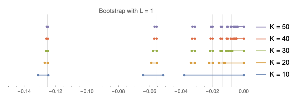
Fig. 1 shows what the regions of validity within the search space look like in practice. The axis is the energy $E$, and the intervals pictured are the regions of allowed values at various depths $K$. The convergence as $K$ grows is apparent. Estimates for the allowed energies can be extracted by simply taking the mean of each region at some high depth $K$. The size of the region in question gives a natural notion of error. We go on to show the bootstrapped spectrum and characterize the convergence of the various intervals as a function of $K$.

References

- (1) X. Han, S.A. Hartnoll and J. Kruthoff, Bootstrapping Matrix Quantum Mechanics, Phys. Rev. Lett. 125 (2020) 041601 [2004.10212].
- (2) S. El-Showk, M.F. Paulos, D. Poland, S. Rychkov, D. Simmons-Duffin and A. Vichi, Solving the 3D Ising Model with the Conformal Bootstrap, Phys. Rev. D 86 (2012) 025022 [1203.6064].
- (3) V. Kazakov and Z. Zheng, Analytic and Numerical Bootstrap for One-Matrix Model and ”Unsolvable” Two-Matrix Model, 2108.04830.
- (4) A. Jevicki, O. Karim, J.P. Rodrigues and H. Levine, Loop Space Hamiltonians and Numerical Methods for Large Gauge Theories, Nucl. Phys. B 213 (1983) 169.
- (5) A. Jevicki, O. Karim, J.P. Rodrigues and H. Levine, Loop Space Hamiltonians and Numerical Methods for Large Gauge Theories. 2., Nucl. Phys. B 230 (1984) 299.
- (6) J.P. Rodrigues, Numerical Solution of Lattice Schwinger-dyson Equations in the Large Limit, Nucl. Phys. B 260 (1985) 350.
- (7) H.W. Lin, Bootstraps to strings: solving random matrix models with positivite, JHEP 06 (2020) 090 [2002.08387].
- (8) H. Hessam, M. Khalkhali and N. Pagliaroli, Bootstrapping Dirac Ensembles, 2107.10333.
- (9) P.D. Anderson and M. Kruczenski, Loop Equations and bootstrap methods in the lattice, Nucl. Phys. B 921 (2017) 702 [1612.08140].
- (10) P. Anderson and M. Kruczenski, Loop equation in Lattice gauge theories and bootstrap methods, EPJ Web Conf. 175 (2018) 11011.
- (11) R.E. Curto and L.A. Fialkow, Recursiveness, positivity, and truncated moment problems, Houston J. Math (1991) 603.
- (12) K. Schmüdgen, The moment problem, vol. 9 of Graduate Texts in Mathematics, Springer (2017).
- (13) F. Cooper, A. Khare and U. Sukhatme, Supersymmetry and quantum mechanics, Phys. Rept. 251 (1995) 267 [hep-th/9405029].