Quantum advantages for Pauli channel estimation
Abstract
We show that entangled measurements provide an exponential advantage in sample complexity for Pauli channel estimation, which is both a fundamental problem and a practically important subroutine for benchmarking near-term quantum devices. The specific task we consider is to simultaneously learn all the eigenvalues of an -qubit Pauli channel to precision. We give an estimation protocol with an -qubit ancilla that succeeds with high probability using only copies of the Pauli channel, while prove that any ancilla-free protocol (possibly with adaptive control and channel concatenation) would need at least rounds of measurement. We further study the advantages provided by a small number of ancillas. For the case that a -qubit ancilla () is available, we obtain a sample complexity lower bound of for any non-concatenating protocol, and a stronger lower bound of for any non-adaptive, non-concatenating protocol, which is shown to be tight. We also show how to apply the ancilla-assisted estimation protocol to a practical quantum benchmarking task in a noise-resilient and sample-efficient manner, given reasonable noise assumptions. Our results provide a practically-interesting example for quantum advantages in learning and also bring new insight for quantum benchmarking.

One important challenge for the Noisy Intermediate-Scale Quantum (NISQ) era Preskill 2018 is to demonstrate quantum advantages on near-term devices. Recent works have made groundbreaking progress towards demonstrating quantum computational advantages Harrow and Montanaro 2017; Arute et al. 2019; Zhong et al. 2020; Wu et al. 2021, which means quantum computers can efficiently solve certain computational problems outside the reach of the most advanced classical computers. However, computation is not the only aspect quantum computers can achieve meaningful advantages. Learning is yet another possibility, where the basic question is whether quantum computers (with resources such as quantum memory and entangled measurements) can help us learn certain properties of a physical system more efficiently. This kind of quantum advantages have been explored by several recent works Bubeck et al. 2020; Aharonov et al. 2021; Huang et al. 2021; Chen et al. 2021a; Rossi et al. 2021 with positive examples including mixedness testing Bubeck et al. 2020, unitarity testing Aharonov et al. 2021, Pauli expectation values estimation Huang et al. 2021, etc. However, all these quantum advantages proposals so far either focus on artificial problems or have no noise-resilient implementation. It is thus highly desirable to identify a practically-interesting learning task that can be used to demonstrate a robust quantum advantage in the NISQ era.
A particularly interesting type of learning tasks, known as quantum benchmarking Eisert et al. 2020, aims at characterizing the noise on a quantum device. This is yet another challenge for the NISQ era which is crucial to building better quantum hardware. Pauli noise is one of the most important quantum noise models: On the one hand, it can describe a wide range of incoherent noise, including dephasing, deplorizing, bit-flip, etc. On the other hand, the recently developed “randomized compiling” technique Wallman and Emerson 2016; Hashim et al. 2020 can tailor any noise model in a universal gate set into Pauli noise. Many benchmarking protocols also rely on twirling the noise into a Pauli channel before extracting any information Erhard et al. 2019; Magesan et al. 2011; Harper et al. 2020; Liu et al. 2021. Because of the important role played by Pauli channels, it is of great interest to study the estimation of these objects in an efficient and practical way. Despite a long line of research Fujiwara and Imai 2003; Hayashi 2010; Chiuri et al. 2011; Ruppert et al. 2012; Collins 2013; Flammia and Wallman 2020; Harper et al. 2021; Flammia and O’Donnell 2021; Mohseni et al. 2008; Flammia and O’Donnell 2021, the ultimate sample complexity for Pauli channel estimation has not yet been fully characterized.
In this work, we demonstrate an exponential quantum advantage for Pauli channel estimation. We show that, for the task of estimating the eigenvalues of an -qubit Pauli channel (i.e., Pauli eigenvalues) to additive error in distance, there exists a measurement protocol assisted with an -qubit ancilla that succeeds with high probability using samples, while any ancilla-free protocol (possibly with adaptive control and channel concatenation) would require at least rounds of measurements. As a byproduct, this provides a lower bound for randomized benchmarking (RB) Magesan et al. 2011; Knill et al. 2008 based Pauli noise estimation protocol, resolving an open problem raised in Flammia and Wallman 2020.
We then study the sample efficiency advantages provided by a restricted amount of ancilla. While an ancilla larger than qubits will not help further improve the efficiency, given a -qubit ancilla, we obtain a lower bound of for any non-concatenating protocol, and a stronger lower bound of for non-adaptive and non-concatenating protocols. The latter is shown to be tight by an explicitly constructed protocol (see Algorithm 1).
Finally, we show how to apply the ancilla-assisted estimation protocol in the practical task of benchmarking Pauli gates. Inspired by RB-type methods Flammia and Wallman 2020; Knill et al. 2008; Magesan et al. 2011, we design a protocol that is both robust against state-preparation-and-measurement (SPAM) errors and exponentially more sample-efficient than any ancilla-free scheme, under reasonable noise assumptions. This protocol can be used to experimentally demonstrate a robust and practical quantum advantage on NISQ devices.
Preliminaries.— For an -qubit Hilbert space, define to be the Pauli group modulo the non-physical phase. is an Abelian group isomorphic to , so we can use elements of to uniquely label elements of . Specifically, we view every as a -bit string corresponding to the Pauli operator
where the phase is chosen to ensure Hermiticity. We also define a sympletic inner product within as
One can verify that Nielsen and Chuang 2011.
An -qubit Pauli channel is a quantum channel of the following form
| (1) |
where is called the Pauli error rates. An important property of Pauli channels is that their eigen-operators are exactly the Pauli operators. Thus, an alternative expression for is
| (2) |
where is called the Pauli eigenvalues Flammia and Wallman 2020; Flammia and O’Donnell 2021. These two sets of parameters, and , are related by the Walsh-Hadamard transform
| (3) |
Both and are physically interesting parameters: The Pauli error rates are directly related to the error thresholds in fault-tolerant quantum computation Shor 1996; Aharonov and Ben-Or 2008 and have been the quantities of interest for many quantum benchmarking protocols Flammia and Wallman 2020; Harper et al. 2020; Harper et al. 2021; Flammia and O’Donnell 2021; Liu et al. 2021; The Pauli eigenvalues quantify how well a Pauli observable is preserved through the noise channel (hence also known as Pauli fidelities) and have applications in quantum error mitigation (see e.g. Chen et al. 2021b). In this work, we will focus on the estimation for .
Comparison of different measurement models.— To study the advantages provided by different kinds of quantum resources, we categorize measurement strategies into ancilla-assisted vs. ancilla-free, concatenating vs. non-concatenating, and adaptive vs. non-adaptive measurements. See Fig. 1 and explanations in the captions. We remark that, recent works on quantum advantages in property learning Huang et al. 2021; Aharonov et al. 2021 have been focusing on the difference between the full-fledged entangled measurement Fig. 1(a) and the un-entangled measurement Fig. 1(d). Here, we introduce two intermediate measurement models Fig. 1(b) and Fig. 1(c) to separately study the role of ancilla and concatenation. There are also practical reasons to care about those intermediate models. As an example, the ancilla-free concatenating measurement model Fig. 1(c) exactly describes most existing RB protocols (see e.g. Helsen et al. 2020), including the RB-type Pauli channel estimation protocol in Ref. Flammia and Wallman 2020. Indeed, we show that it is the ancilla that provides an exponential advantage in sample complexity for Pauli channel estimation, while concatenation does not help improve the sample efficiency. These results further advances our understanding of quantum advantages in property learning Huang et al. 2021; Aharonov et al. 2021; Bubeck et al. 2020; Chen et al. 2021a.
Regarding these measurement models, one further question to ask is whether a restricted amount of ancilla can provide any sample efficiency advantages. In this work, we will characterize the advantages provided by a -qubit ancilla () for the non-concatenating measurement models. This kind of quantitative trade-off relations between quantum resources and sample efficiency has not been explored in previous works Huang et al. 2021; Aharonov et al. 2021; Bubeck et al. 2020; Chen et al. 2021a and may potentially lead to a new resource-theoretical interpretation of quantum entanglement Chitambar and Gour 2019.
Upper bounds.— Our goal is to estimate the Pauli eigenvalues of an -qubit Pauli channel to precision in distance, i.e., estimating each to additive error.
When an -qubit ancillary system is available, a simple protocol is as follows: prepare Bell pairs, input one qubit from each pair to the Pauli channel, and apply a Bell measurement on the output. Since the Pauli channel can be viewed as randomly applying one of the Pauli operators with probability , and each is mapped to a unique measurement outcome 11 1 This can be viewed as a consequence of the well-known superdense coding protocol Bennett and Wiesner 1992. , we are effectively sampling from the probability distribution . The sample of can then be used to construct an estimator for according to the Walsh-Hadamard transform. As shown in Theorem 1, this protocol has sample complexity ; on the other hand, when no ancilla is allowed, there is no way to sample from and simultaneously estimate all elements of from a single measurement setting. Intuitively, this is what makes the task difficult.
In the following, we give a unified estimation protocol using ancilla qubits for . Roughly speaking, we divide the qubits of the Pauli channel into two disjoint subsystems containing and qubits, respectively, and deal with them separately. For the first subsystem, we introduce a -qubit ancilla, input Bell pairs to both systems, and apply a Bell measurement; For the second subsystem, we will use stabilizer states input and syndrome measurements to be defined later. The measurement scheme is depicted in Fig. 2.
A rigorous description of the protocol is given in Algorithm 1. Here, represents the Bell states on the -qubit subsystem defined as
| (4) |
A stabilizer group on the ()-qubit subsystem is a group of commuting Pauli operators. Mathematically, can be viewed as an ()-dimensional subspace of . The stabilizer states are the simultaneous eigenstates of all Pauli operators in , which can be expressed as
| (5) |
for known as the error syndrome. Note that forms an orthonormal basis for the -qubit subsystem. The stabilizer covering is a set of stabilizer groups such that every Pauli operator belongs to at least one Flammia and Wallman 2020.

Theorem 1.
Algorithm 1 gives an estimate for the Pauli eigenvalues of any -qubit Pauli channels that satisfies
| (6) |
with success probability at least , given the following number of samples
| (7) |
Proof of Theorem 1.
The probability distribution of measurement outcomes at Line 5 in Algorithm 1 can be calculated as
| (8) |
See the supplemental material for more details. Therefore, and are related by the Walsh-Hadamard transform. Taking the inverse transform, we get
| (9) |
Thus, is an un-biased estimator of . According to Hoeffding’s bound, samples are enough to estimate a single to additive precision with success probability at least . Since every is covered by some stabilizer group , a total sample complexity of is enough to estimate all to additive error simultaneously with success probability at least , by setting and applying the union bound. ∎
Corollary 2.
There exists a -qubit-ancilla-assisted non-adaptive non-concatenating Pauli channel estimation protocol achieving for all with probability using samples.
Proof.
This follows from the existence of a stabilizer covering for of size Lawrence et al. 2002, which in turn follows from the existence of mutually-unbiased bases for -qubit systems Wootters and Fields 1989. ∎
We remark that, the choice of stabilizer covering in Corollary 2 gives the optimal sample complexity for all non-adaptive and non-concatenating Pauli eigenvalues estimation protocols, as proved in the next section. From a practical point of view, it involves -qubit stabilizer states that might be difficult to prepare. A more experimental friendly version is to choose the stabilizer covering generated by all possible Pauli measurements, in which case only Pauli eigenstates preparation and Pauli measurements are required (on the -qubit subsystem), at the expense of a sub-optimal sample complexity .
Lower bounds.— We have established a sample complexity upper bound of for non-adaptive non-concatenating k-qubit-ancilla-assisted Pauli eigenvalues estimation protocols, which implies a upper bound for the -qubit ancilla case and a upper bound for the ancilla-free case. In the following Theorem 3, we provide corresponding lower bounds to justify the exponential advantage provided by ancilla in this task.
Theorem 3.
For any estimation protocol that give an estimate for the Pauli eigenvalues of an arbitrary unknwon -qubit Pauli channel such that
| (10) |
holds with high probability, the number of samples of must satisfies (recall Fig. 1)
- (A)
, for non-adaptive non-concatenating k-qubit-ancilla measurements.
- (B)
, for adaptive non-concatenating k-qubit-ancilla measurements.
- (C)
, for adaptive concatenating ancilla-free measurements, where stands for the number of measurement rounds.
- (D)
, for fully entangled measurements.
Indeed, Theorem 3 and Corollary 2 establishes an exponential advantage of ancilla-assisted measurements over ancilla-free measurements even with channel concatenation (as in the RB-type Pauli channel estimation protocols in Ref. Flammia and Wallman 2020). Furthermore, for the non-concatenating cases, we see a roughly matching bounds for all ancilla size , which can be interpreted as that a small number of ancilla () would not help much in improving the sample efficiency. We also see from (D) that the sample complexity of Algorithm 1 with ancilla qubits is optimal among all entangled strategies, thus we need not study protocols with more than ancilla qubits.
Sketch of the proof.
Our proof generalizes the techniques of Huang et al. Huang et al. 2021 in proving lower bounds for learning Pauli expectation values of quantum states. The key is to construct the following set of Pauli channels
| (11) |
for and . An estimation protocol satisfying the assumption of Theorem 3 is able to identify an arbitrary element of this set using copies of the channel. We can then use information-theoretical arguments to lower bound for (A); The bounds in (B) and (C) are proved by reducing the learning problem to a channel discrimination problem between the completely-deplorizing channel and the channels in Eq. (11); To prove the bound in (D), we first use teleportation stretching Pirandola et al. 2017; Pirandola et al. 2019 to reduce any estimation protocols on copies of the Pauli channel into a POVM measurement on copies of their Choi states Choi 1975; Jamiołkowski 1972, and then apply the Holevo’s theorem Holevo 1973. See the supplemental material for a full proof of Theorem 3. ∎
Applications in quantum benchmarking.— The estimation protocol we described earlier is based on an ideal situation where we have direct access to the Pauli channel of interest and ignore the state preparation and measurement (SPAM) error. In the supplemental material, we introduce a quantum benchmarking protocol for the Pauli gates, which can be viewed as an extension of Algorithm 1. The protocol uses an -qubit ancilla and (possibly imperfect) Bell state preparation and measurements. However, the application of the Pauli channel in Fig. 2 is now replaced by applying a sequence of random Pauli gates to be characterized, as shown in Fig. 3. By repeating this procedure for different sequence lengths, we reduce the sensitivity to SPAM errors. In addition to robustness against SPAM errors, this protocol provides an exponential advantage in sample complexity compared to any ancilla-free protocol, as long as the ancillary system has a long coherence time and is well isolated from the main system, among other reasonable noise assumptions. These assumptions can potentially be satisfied by e.g., an ion trap platform Wright et al. 2019; Pino et al. 2021.

Summary and outlook.— In this work, we show a provable quantum advantage provided by entangled measurements for a learning task Aharonov et al. 2021; Huang et al. 2021 of Pauli channel estimation, which is a practically useful tool urgently needed to characterize large quantum systems. For quantum benchmarking, our results provide fundamental efficiency limits for Pauli noise estimation, which partly solve an open problem raised in Flammia and Wallman 2020. We also describe how the ancilla-assisted Pauli channel estimation protocol can be applied to a practical quantum benchmarking tasks in a noise-resilient and sample-efficient manner. Our results provide a promising tool for both characterizing near-term quantum devices and demonstrating quantum advantages in those systems
Several interesting questions remain to be explored in the future, including exploring the quantum advantages in learning other properties of Pauli channels (e.g., the Pauli error rates 22 2 It is shown in Flammia and O’Donnell 2021 that the Pauli error rates for an -qubit Pauli channel can be estimated to small error in distance using un-entangled measurements with samples, so there is no large advantages for entangled strategies. Still, one could expect a sample-efficiency advantage under other practically-interesting metric of estimation precision. ); analyzing the sample complexity for learning Pauli channels with more specific structures; and analyzing the experimental performance of our algorithms in comparison to other ancilla-free protocols Harper et al. 2020; Hashim et al. 2020.
Acknowledgements.
We acknowledge support from the ARO (W911NF-18-1-0020, W911NF-18-1-0212), ARO MURI (W911NF-16-1-0349), AFOSR MURI (FA9550-19-1-0399, FA9550-21-1-0209), DoE Q-NEXT, NSF (EFMA-1640959, OMA-1936118, EEC-1941583), NTT Research, and the Packard Foundation (2013-39273). S.Z. acknowledges funding provided by the Institute for Quantum Information and Matter, an NSF Physics Frontiers Center (NSF Grant PHY-1733907). A.S. is supported by a Chicago Prize Postdoctoral Fellowship in Theoretical Quantum Science.References
- Preskill (2018) J. Preskill, Quantum computing in the nisq era and beyond, Quantum 2, 79 (2018).
- Harrow and Montanaro (2017) A. W. Harrow and A. Montanaro, Quantum computational supremacy, Nature 549, 203 (2017).
- Arute et al. (2019) F. Arute, K. Arya, R. Babbush, D. Bacon, J. C. Bardin, R. Barends, R. Biswas, S. Boixo, F. G. Brandao, D. A. Buell, et al., Quantum supremacy using a programmable superconducting processor, Nature 574, 505 (2019).
- Zhong et al. (2020) H.-S. Zhong, H. Wang, Y.-H. Deng, M.-C. Chen, L.-C. Peng, Y.-H. Luo, J. Qin, D. Wu, X. Ding, Y. Hu, et al., Quantum computational advantage using photons, Science 370, 1460 (2020).
- Wu et al. (2021) Y. Wu, W.-S. Bao, S. Cao, F. Chen, M.-C. Chen, X. Chen, T.-H. Chung, H. Deng, Y. Du, D. Fan, et al., Strong quantum computational advantage using a superconducting quantum processor, arXiv preprint arXiv:2106.14734 (2021).
- Bubeck et al. (2020) S. Bubeck, S. Chen, and J. Li, Entanglement is necessary for optimal quantum property testing, in 2020 IEEE 61st Annual Symposium on Foundations of Computer Science (FOCS) (IEEE, 2020) pp. 692–703.
- Aharonov et al. (2021) D. Aharonov, J. Cotler, and X.-L. Qi, Quantum algorithmic measurement, arXiv preprint arXiv:2101.04634 (2021).
- Huang et al. (2021) H.-Y. Huang, R. Kueng, and J. Preskill, Information-theoretic bounds on quantum advantage in machine learning, Phys. Rev. Lett. 126, 190505 (2021).
- Chen et al. (2021a) S. Chen, J. Li, and R. O’Donnell, Toward instance-optimal state certification with incoherent measurements, arXiv preprint arXiv:2102.13098 (2021a).
- Rossi et al. (2021) Z. M. Rossi, J. Yu, I. L. Chuang, and S. Sugiura, Quantum advantage for noisy channel discrimination, arXiv preprint arXiv:2105.08707 (2021).
- Eisert et al. (2020) J. Eisert, D. Hangleiter, N. Walk, I. Roth, D. Markham, R. Parekh, U. Chabaud, and E. Kashefi, Quantum certification and benchmarking, Nature Reviews Physics 2, 382 (2020).
- Wallman and Emerson (2016) J. J. Wallman and J. Emerson, Noise tailoring for scalable quantum computation via randomized compiling, Physical Review A 94, 052325 (2016).
- Hashim et al. (2020) A. Hashim, R. K. Naik, A. Morvan, J.-L. Ville, B. Mitchell, J. M. Kreikebaum, M. Davis, E. Smith, C. Iancu, K. P. O’Brien, et al., Randomized compiling for scalable quantum computing on a noisy superconducting quantum processor, arXiv preprint arXiv:2010.00215 (2020).
- Erhard et al. (2019) A. Erhard, J. J. Wallman, L. Postler, M. Meth, R. Stricker, E. A. Martinez, P. Schindler, T. Monz, J. Emerson, and R. Blatt, Characterizing large-scale quantum computers via cycle benchmarking, Nature communications 10, 1 (2019).
- Magesan et al. (2011) E. Magesan, J. M. Gambetta, and J. Emerson, Scalable and robust randomized benchmarking of quantum processes, Physical review letters 106, 180504 (2011).
- Harper et al. (2020) R. Harper, S. T. Flammia, and J. J. Wallman, Efficient learning of quantum noise, Nature Physics 16, 1184 (2020).
- Liu et al. (2021) Y. Liu, M. Otten, R. Bassirianjahromi, L. Jiang, and B. Fefferman, Benchmarking near-term quantum computers via random circuit sampling, arXiv preprint arXiv:2105.05232 (2021).
- Fujiwara and Imai (2003) A. Fujiwara and H. Imai, Quantum parameter estimation of a generalized pauli channel, Journal of Physics A: Mathematical and General 36, 8093 (2003).
- Hayashi (2010) M. Hayashi, Quantum channel estimation and asymptotic bound, in Journal of Physics: Conference Series, Vol. 233 (IOP Publishing, 2010) p. 012016.
- Chiuri et al. (2011) A. Chiuri, V. Rosati, G. Vallone, S. Pádua, H. Imai, S. Giacomini, C. Macchiavello, and P. Mataloni, Experimental realization of optimal noise estimation for a general pauli channel, Physical review letters 107, 253602 (2011).
- Ruppert et al. (2012) L. Ruppert, D. Virosztek, and K. Hangos, Optimal parameter estimation of pauli channels, Journal of Physics A: Mathematical and Theoretical 45, 265305 (2012).
- Collins (2013) D. Collins, Mixed-state pauli-channel parameter estimation, Physical Review A 87, 032301 (2013).
- Flammia and Wallman (2020) S. T. Flammia and J. J. Wallman, Efficient estimation of pauli channels, ACM Transactions on Quantum Computing 1, 1 (2020).
- Harper et al. (2021) R. Harper, W. Yu, and S. T. Flammia, Fast estimation of sparse quantum noise, PRX Quantum 2, 010322 (2021).
- Flammia and O’Donnell (2021) S. T. Flammia and R. O’Donnell, Pauli error estimation via population recovery, Quantum 5, 549 (2021).
- Mohseni et al. (2008) M. Mohseni, A. T. Rezakhani, and D. A. Lidar, Quantum-process tomography: Resource analysis of different strategies, Physical Review A 77, 032322 (2008).
- Knill et al. (2008) E. Knill, D. Leibfried, R. Reichle, J. Britton, R. B. Blakestad, J. D. Jost, C. Langer, R. Ozeri, S. Seidelin, and D. J. Wineland, Randomized benchmarking of quantum gates, Physical Review A 77, 012307 (2008).
- Nielsen and Chuang (2011) M. A. Nielsen and I. L. Chuang, Quantum Computation and Quantum Information: 10th Anniversary Edition, 10th ed. (Cambridge University Press, USA, 2011).
- Shor (1996) P. W. Shor, Fault-tolerant quantum computation, in Proceedings of 37th Conference on Foundations of Computer Science (IEEE, 1996) pp. 56–65.
- Aharonov and Ben-Or (2008) D. Aharonov and M. Ben-Or, Fault-tolerant quantum computation with constant error rate, SIAM Journal on Computing 10.1137/S0097539799359385 (2008).
- Chen et al. (2021b) S. Chen, W. Yu, P. Zeng, and S. T. Flammia, Robust shadow estimation, PRX Quantum 2, 030348 (2021b).
- Helsen et al. (2020) J. Helsen, I. Roth, E. Onorati, A. H. Werner, and J. Eisert, A general framework for randomized benchmarking, arXiv preprint arXiv:2010.07974 (2020).
- Chitambar and Gour (2019) E. Chitambar and G. Gour, Quantum resource theories, Reviews of Modern Physics 91, 025001 (2019).
- (34) This can be viewed as a consequence of the well-known superdense coding protocol Bennett and Wiesner 1992.
- Lawrence et al. (2002) J. Lawrence, Č. Brukner, and A. Zeilinger, Mutually unbiased binary observable sets on n qubits, Physical Review A 65, 032320 (2002).
- Wootters and Fields (1989) W. K. Wootters and B. D. Fields, Optimal state-determination by mutually unbiased measurements, Annals of Physics 191, 363 (1989).
- Pirandola et al. (2017) S. Pirandola, R. Laurenza, C. Ottaviani, and L. Banchi, Fundamental limits of repeaterless quantum communications, Nature communications 8, 1 (2017).
- Pirandola et al. (2019) S. Pirandola, R. Laurenza, C. Lupo, and J. L. Pereira, Fundamental limits to quantum channel discrimination, npj Quantum Information 5, 1 (2019).
- Choi (1975) M.-D. Choi, Completely positive linear maps on complex matrices, Linear algebra and its applications 10, 285 (1975).
- Jamiołkowski (1972) A. Jamiołkowski, Linear transformations which preserve trace and positive semidefiniteness of operators, Reports on Mathematical Physics 3, 275 (1972).
- Holevo (1973) A. S. Holevo, Bounds for the quantity of information transmitted by a quantum communication channel, Problemy Peredachi Informatsii 9, 3 (1973).
- Wright et al. (2019) K. Wright, K. Beck, S. Debnath, J. Amini, Y. Nam, N. Grzesiak, J.-S. Chen, N. Pisenti, M. Chmielewski, C. Collins, et al., Benchmarking an 11-qubit quantum computer, Nature communications 10, 1 (2019).
- Pino et al. (2021) J. M. Pino, J. M. Dreiling, C. Figgatt, J. P. Gaebler, S. A. Moses, M. Allman, C. Baldwin, M. Foss-Feig, D. Hayes, K. Mayer, et al., Demonstration of the trapped-ion quantum ccd computer architecture, Nature 592, 209 (2021).
- (44) It is shown in Flammia and O’Donnell 2021 that the Pauli error rates for an -qubit Pauli channel can be estimated to small error in distance using un-entangled measurements with samples, so there is no large advantages for entangled strategies. Still, one could expect a sample-efficiency advantage under other practically-interesting metric of estimation precision.
- Bennett and Wiesner (1992) C. H. Bennett and S. J. Wiesner, Communication via one-and two-particle operators on einstein-podolsky-rosen states, Physical review letters 69, 2881 (1992).
- Flammia et al. (2012) S. T. Flammia, D. Gross, Y.-K. Liu, and J. Eisert, Quantum tomography via compressed sensing: error bounds, sample complexity and efficient estimators, New Journal of Physics 14, 095022 (2012).
- Haah et al. (2017) J. Haah, A. W. Harrow, Z. Ji, X. Wu, and N. Yu, Sample-optimal tomography of quantum states, IEEE Transactions on Information Theory 63, 5628 (2017).
- Roth et al. (2018) I. Roth, R. Kueng, S. Kimmel, Y.-K. Liu, D. Gross, J. Eisert, and M. Kliesch, Recovering quantum gates from few average gate fidelities, Physical review letters 121, 170502 (2018).
- Cover and Thomas (2012) T. M. Cover and J. A. Thomas, Elements of Information Theory (John Wiley & Sons, 2012).
- Bennett et al. (1996) C. H. Bennett, D. P. DiVincenzo, J. A. Smolin, and W. K. Wootters, Mixed-state entanglement and quantum error correction, Physical Review A 54, 3824 (1996).
- Wilde (2013) M. M. Wilde, Quantum information theory (Cambridge University Press, 2013).
Appendix A Details about the proof of Theorem 1
In this section, we provide details in the derivation of Eq. (8), i.e., the distribution of measurement outcomes at Line 5 in Algorithm 1. For clarity, denote the -qubit Hilbert space of the ancilla as , and divide the -qubit Hilbert space of the main system into a -qubit subspace and an ()-qubit subspace . The input state to the channel is and the measurement basis is Here, are Bell states and can be expressed as
| (12) | ||||
And the stabilizer state is defined as
| (13) |
for . We remark that, the stabilizer state is well-defined for all , but and represent the same state if (bitwise modulo 2 sum), so we only need to consider the quotient space of over . When calculating the sympletic inner product , one should understand as an arbitrary representative of the coset it stands for.
Therefore, the measurement outcome distribution can be calculated as
| (14) | ||||
which is exactly Eq. (8) in the main text. It is then obvious that and are related by the Walsh-Hadamard transform (see (Flammia and Wallman 2020, Lemma 4)).
Appendix B Proof of the lower bounds
B.1 A tight lower bound for non-adaptive and non-concatenating strategies
In this section, we prove a matching lower bound of for all non-adaptive and non-concatenating k-qubit ancilla-assisted Pauli channel estimation protocols, which include the ancilla-free strategies () and -qubit ancilla assisted strategies () as two special cases. Recall that, by a non-adaptive and non-concatenating protocol we mean that, for each sample of the Pauli channel , we prepare an qubits state, input it to , and apply a POVM measurement on the joint output state. The input state and measurement setting for the th sample is not allowed to depend on previous measurement outcomes, nor do we allow concatenating multiple samples of in a single round of measurement (which is used in RB-type Pauli error estimation protocols Flammia and Wallman 2020).
Theorem 4.
For any non-adaptive, non-concatenating -qubit ancilla-assisted protocols that give an estimate of the Pauli eigenvalues of an arbitrary unknown -qubit Pauli channel such that
| (15) |
holds with high probability, the number of samples of required is at least .
Our proof techniques generalize the information-theoretical arguments by Huang et al. Huang et al. 2021, which in turn stem from previous work on sample complexity lower bounds for quantum tomography Flammia et al. 2012; Haah et al. 2017; Roth et al. 2018. Consider a communication protocol between Alice and Bob where their share the following “codebook”:
| (16) |
Now, Alice picks at uniform random one out of the possible pairs of and then send copies of the channel to Bob. If there exists a Pauli channel estimation protocol using samples and satisfying the assumption of Theorem 4, Bob can use that protocol to uniquely determine Alice’s choice of with high probability, since the Pauli eigenvalues of any only take values from . Suppose Bob’s input state and POVM outcome for the th sample is . According to Fano’s inequality, the mutual information between the random variable pair and Bob’s measurement results has the following lower bound
| (17) |
We also know by assumption that the measurement outcomes are independent from each other, conditioned on . The chain rule of mutual information then gives that
| (18) |
We will show that in the following lemma. This would then give us the desired sample complexity lower bound , which completes the proof of Theorem 4.
Lemma 5.
Proof.
First notice that it suffices to consider pure state input and rank- POVM measurements. The latter comes from the fact that every POVM measurement can be viewed as a coarse-graining of some rank-1 POVM measurement. To see the former, consider the underlying distribution . The mutual information is convex about when fixing (see e.g., (Cover and Thomas 2012, Theorem 2.7.4)), thus using mixed state input can never provide a larger mutual information.
Thanks to this observation, we can without loss of generality let the input state be and let the POVM measurement be , where are unit vectors, and by normalization. We also abuse notations a little bit to let and denote the matrices that satisfy
| (19) |
where and are computational basis states. The normalization condition of and is equivalent to
| (20) |
We also define which is a matrix of rank less or equal to .
The mutual information between and a single round of measurement outcome can be upper bounded as
| (21) | ||||
where the inequality follows from the fact that in which we take and .
The conditional probability can be calculated as
| (22) | ||||
where we expand the identity channel as in the second line, and use the fact equals to the swap operator in the fourth line.
The average value and second moment of according to the distribution of are
| (23) | ||||
Hence we have the following bound for the mutual information
| (24) |
Now we further calculate the R.H.S. of the above inequality. Let . Notice that
| (25) |
which means there exists a rank- projector such that . According to Cauchy-Schwarz inequality,
| (26) | ||||
Substitute this into Eq. (24),
| (27) | ||||
where the third line uses the following formula of Pauli twirling,
| (28) |
and the last line follows from the fact that
| (29) |
This completes the proof of Lemma 5. ∎
B.2 A lower bound for adaptive but non-concatenating strategies
In this section, we prove a (perhaps loose) lower bound of for all adaptive and non-concatenating -qubit ancilla-assisted Pauli channel estimation protocols, as stated in the following theorem.
Theorem 6.
For any adaptive, non-concatenating -qubit ancilla-assisted protocols that give an estimate of the Pauli eigenvalues of an arbitrary unknown -qubit Pauli channel such that
| (30) |
holds with high probability, the number of samples of required is at least .
Our proof techniques generalize the methods of Huang et al. Huang et al. 2021 for proving adaptive sample complexity lower bounds for Pauli expectation values estimation of unknown quantum states. Consider the following possible Pauli channels
| (31) |
Here is known as the completely deplorizing channel. If there exists an Pauli channel estimation protocol satisfying the requirement of Theorem 6, one can unambiguously identify each one of the possible Pauli channels appearing above with high probability, given sufficient number of samples of . This in turn implies that one should be able to distinguish the following two equal-probable hypotheses with high success probability.
- 1.
Given copies of .
- 2.
Given copies of for a uniformly-randomly picked .
For an adaptive but non-concatenating protocol, one has to choose an dimensional input state and a POVM measurement for the th sample of , where the choice may depend on previous measurement outcomes. Denote the measurement outcome of the th round as . We explicitly write the state and measurement at the th round as and to emphasize their dependence on .Denote the measurement outcomes among all the samples as . The probability distribution of under the above two hypothesis can be expressed as
| (32) |
The ability to distinguish these two hypotheses is equivalent to the ability to distinguish from . The maximal success probability of distinguishing two probability distributions is given by where stands for the total variance distance defined as follows
| (33) |
We will show in the following Lemma that , which immediately implies that one must have in order to obtain high success probability in distinguishing from . This then completes the proof of Theorem 6.
Lemma 7.
.
Proof.
First notice that it suffices to consider pure state input and rank- POVM measurement. For the former, the probability distribution obtained from mixed state input can be viewed as a convex combination of distributions obtained from pure state input. Thanks to the joint convexity, mixed state input can not yield a larger total variance distance; For the latter, every POVM measurement can be viewed as a coarse-graining of some rank- POVM measurement. Because of the data-processing property, this coarse-graining would not yield a larger total variance distance.
In light of this observation, we can without loss of generality let the input state at the th round be and let the POVM measurement be , conditioned on previous measurement outcomes , where are unit vectors, and by normalization. We also introduce the two matrices defined similarly as in Eq. (19), and define which is a matrix of rank less or equal to . With the above definitions, one can verify that and can be expressed as follows
| (34) | ||||
The total variance between and can then be bounded as
| (35) | ||||
In order to bound the R.H.S., we make use of a technique from Huang et al. Huang et al. 2021. Let denote an arbitrary complex matrix of rank no more than , consider the following subset of -qubit Pauli operators
| (36) |
We claim that the size of satisfies
| (37) |
which can be shown by contradiction: Suppose this does not hold, we would have
| (38) | ||||
However, the L.H.S. of the above can be upper bounded as
| (39) | ||||
where the first inequality follows from Cauchy-Schwarz (see Eq. (26)), and the first equality evaluates the Pauli twirling (see Eq. (27)). This leads to contradition, and hence proves the desired lower bound on .
Now, we define another subset of -qubit Pauli operators, conditioned on the measurement outcomes , as follows
| (40) |
By applying a “union bound” on Eq. (36), we immediately have the following lower bound on the size of :
| (41) |
We are now ready to upper bound from Eq. (35). The strategy is to divide the sum over all Pauli operators into and . All terms within the former group are small thanks to the definition of ; Terms within the latter group could be large, but the total number of them are small. Combining these two gives a pretty good upper bound on . In math,
| (42) | ||||
The first inequality uses an additional fact that to bound the second sum, which follows from the Cauchy-Schwarz inequality. The second inequality uses the bounds for the first sum and Eq. (41) for the second sum, as well as the fact that for all . (Note that only if , but our targeted upper bound trivially holds for .) This completes the proof of Lemma 7.
∎
B.3 A lower bound for the most general ancilla-free strategies
The lower bounds in the previous sections work for non-concatenating strategies, where one is not allowed to concatenate (or, coherently access) multiple copies of the unknwon channel before doing a single measurement. The concatenating strategies, as depicted in Fig. 1, are however a natural apparatus for many randomized benchmarking protocols, where one effectively concatenate a varying number of noise channels in order to measure a series of exponentially-decaying values, and then extract the parameters of interest via fitting the decay rate. The original purpose of such concatenation in these protocols is to eliminate the effect of state-preparation-and-measurement (SPAM) error. Here, we want to understand whether concatenating strategies also provide a sample complexity advantage. The short answer is no. We will present a sample complexity lower bound of for the most powerful (adaptive, concatenating) ancilla-free () Pauli channel estimation schemes. This result justifies our claim that ancillary systems are indeed indispensable to overcome the exponential barrier in sample complexity.
To start with, we give a rigorous definition of the most general ancilla-free strategies that we are going to study
Definition 1.
Let be an unknwon -qubit Pauli channel. An adaptive, concatenating, ancilla-free estimation protocol is specified by the following parameters. Let denote the total rounds of measurements. For the th round, let denote the input state, denote the POVM measurement, denote the length of concatenation, and denote a set of processing channels. The th measurement outcome is given by with probability
| (43) |
All the superscript are used to emphasize the dependence on previous measurement outcomes. The protocol should produce an estimate of via classical processing on the measurement outcomes .
The problem we are interested in is still approximating the Pauli eigenvalues to small error in distance. Note that, the parameter in the above definition is not exactly the sample complexity but is the total number of measurements conducted. Since one is allowed to concatenate multiple copies of in a single measurement, is a lower bound for the sample complexity of . Our result is summarized in the following theorem.
Theorem 8.
For any adaptive, concatenating, ancilla-free protocols that gives an estimate of the Pauli eigenvalues of an arbitrary unknown -qubit Pauli channel such that
| (44) |
holds with high probability, the rounds of measurements (and hence the number of samples of ) required is at least .
Proof.
The proof methods are similar to the proof of Theorem 6. Define the following Pauli channels.
| (45) |
We consider the problem of distinguishing the following two equal-probable hypotheses
- 1.
Given copies of .
- 2.
Given copies of for a uniformly-randomly picked .
An estimation protocol satisfying our assumptions should be able to distinguish these two hypotheses with high probability. Let the probability distribution of the measurement outcomes under these two hypotheses be and , respectively. The total variance distance must be at least for the distinguishing task to succeed with high probability. We will show in the following that , which then gives the claimed lower bound of .
To start with, based on the same argument as in the proof of Lemma 7, it suffices to consider pure state input and rank- POVM measurements, so we replace and in Definition 1 with and respectively, where are unit vectors, and by normalization.
Next, we calculate the distribution of under the two different hypotheses. The expression for can be easily obtained, as is simply the completely deplorizing channel. We have
| (46) | ||||
The expression for is more complicated. We first define the following recursive expression
| (47) |
The expression for can then be calculated as follows
| (48) | ||||
The third line uses the fact that is trace-preserving. The total variance distance between and is then
| (49) | ||||
We now need a bound of , which can be shown by induction. We see by definition. Suppose , we have
| (50) | ||||
The first line is by the defining recursive expression; The second line is by the tracial matrix Hölder inequality; The third line uses the fact that is a positive map, and that is positive semidefinite thanks to the induction hypothesis . Thus we can remove the modulus within the trace, and also remove as it is trace-preserving. By induction, we’ve shown .
The remaining part of bounding is basically the same as in the proof of Lemma 7. We repeat it here for completeness. Let be any -qubit pure state. Consider the following subset of -qubit Pauli operators
| (51) |
We claim that the size of satisfies
| (52) |
which can be shown by contradiction: Suppose this does not hold, we would have
| (53) | ||||
However, the L.H.S. of the above can be calculated as
| (54) |
This leads to contradition, and hence proves the desired lower bound on .
Now, we define another subset of -qubit Pauli operators, conditioned on the measurement outcomes , as follows
| (55) |
By applying a “union bound” on Eq. (51), we immediately have the following lower bound on the size of :
| (56) |
We are now ready to upper bound from Eq. (49). The strategy is to divide the sum over all Pauli operators into and . All terms within the former group are small thanks to the definition of ; Terms within the latter group could be large, but the total number of them are small. Combining these two gives a pretty good upper bound on . In math,
| (57) | ||||
The first inequality applies the bound . Besides, the first sum uses the bound from the definition of , and the second sum is bounded using . The second inequality uses the bounds for the first sum and Eq. (56) for the second sum, as well as the fact that for all . Now we have obtained the claimed bound , and hence complete the proof of Theorem 8. ∎
B.4 A lower bound for the most general entangled strategies
In this section, we prove a lower bound of for the fully entangled estimation strategies, which is the most general measurement strategies one can do to learn an unknown channel even with the help of quantum computers, see Fig. 1 (a). Note that, since we assume there is an unlimited amount of quantum memory, we can without loss of generality eliminate any intermediate measurements, and only conduct one joint measurement after sequentially processing all samples of the channel.
Theorem 9.
For any fully entangled measurement protocols that give an estimate for the Pauli eigenvalues of an arbitrary unknown -qubit Pauli channel such that
| (58) |
holds with high probability, the number of samples of required is at least .
Proof.
We first show that, by using a technique known as teleportation stretching Pirandola et al. 2017; Pirandola et al. 2019, any fully entangled measurement protocols for copies of an arbitrary Pauli channel can be simulated by a joint measurement on copies of the Choi state which is defined as
| (59) | ||||
This follows from the existence of a quantum channel such that holds for all Pauli channels . One possible construction of is shown in Fig. 4 (see Ref. Bennett et al. 1996). In word, one first applies a Bell measurement on the input state and half of the Choi state . Then, conditioned on the Bell measurement outcome , one applies a Pauli correction on the other half of , which will then be equal to . Indeed, the post-measurement state conditioned on Bell measurement outcome is
| (60) | ||||
After applying the Pauli correction, the state becomes
| (61) |
which justify the relation .
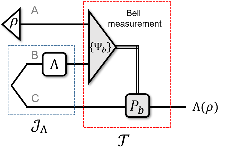
With the help of teleportation stretching, one can reduce any measurement protocols for copies of to a single POVM measurement on copies of , as shown in Fig. 5.

Now, recall the communication task defined in Sec. B.1, where Alice and Bob share the following “codebook”
| (62) |
and Alice randomly picks one possible and send copies of to Bob. If there exists a fully entangled estimation protocol using samples and satisfying the assumption of Theorem 9, Bob can determine Alice’s choice of with high probability. According to Fano’s inequality, the mutual information between the random variable pair and Bob’s measurement result has the following lower bound
| (63) |
One the other hand, since any measurement Bob conducts can be simulated by a measurement on copies of , Holevo’s theorem Holevo 1973; Wilde 2013 can be apply to . We have
| (64) | ||||
In the third line, the first term is a trivial upper bound for the von Neumann entropy on a -dimensional Hilbert space. The second term uses the observation that
| (65) |
is a maximally mixed state on a -dimensional Hilbert space, thus . This yields the lower bound . ∎
Appendix C SPAM-robust ancilla-assisted Pauli gate benchmarking protocols
In the main text, we have described an ancilla-assisted Pauli channel estimation protocol which provides exponential advantages over any ancilla-free protocols. Several issues need to be addressed before applying these protocols to a practical quantum noise characterization setting. Firstly, in most cases, we do not have a “black-box” access to the Pauli noise channels of interest. Instead, they are often attached with some applied quantum gates. We must consider the effect of such gates in our protocol. Secondly, the state preparation and measurement (SPAM) process would inevitably suffer from error. We would like to minimize the effect of such errors.
A recent breakthrough by Flammia and Wallman Flammia and Wallman 2020 provides a way to address these issues, using ideas from randomized benchmarking (see Helsen et al. 2020 and references therein). Their task is to benchmark the Pauli error rates of the Pauli gate set. By concatenating layers of random Pauli gates, they effectively obtain the th power of the Pauli twirl for the noise channel (plus a single Pauli correction gate at the end), under a gate-independent, time-stationary, and Markovian (GTM) noise assumption. They then describe a protocol to estimate the quantity for all , where is the Pauli eigenvalues of the noise channel of interest, and is a SPAM related constant that is independent of . By repeating this estimation procedure for different concatenating length and applying a single-exponential fitting of for each , one obtained an SPAM-robust estimation for .
Importantly, the protocol in Flammia and Wallman 2020 is ancilla-free, which means an exponential number of measurements is necessary to approximate to small error in distance, according to our Theorem 3 (C). In this section, we explain how the ancilla-assisted Pauli channel estimation protocol described in the main text can be extended to this Pauli gates benchmarking setting, which is able to estimate exponentially more sample-efficiently as well as being SPAM-robust. The new protocol uses gate concatenation and single-exponential fitting, and can be viewed as a generalization of the methods in Flammia and Wallman 2020.
Let us start by defining the task and specifying our assumptions. The task is to characterize the noise of the -qubit Pauli gate set. We assume the noise satisfies the GTM condition, which means every noisy implementation of Pauli gates can be written as
| (66) |
for an -independent quantum channel . The calligraphic is the channel representation of the Pauli gate , i.e., . Our specific goal is to estimate the Pauli eigenvalues of the Pauli twirl of , which is defined as
| (67) |
In addition, we assume there to be an -qubit ancillary systems that can be entangled with the main system. The ancilla will basically be used as a quantum memory (see Fig. 3 in the main text). A crucial assumption we need is that, the noise on the ancilla is negligible except for the entangled state preparation and measurement procedure. In other word, the noise channel on the ancilla is independent of the concatenating length on the main system. In practice, this requires (1) the crosstalk between the ancilla and the main system is negligible when applying gates only on the main system, and (2) the coherence time of the ancilla is much longer compared to the time of applying gates on the main system. We expect that these assumptions can be satisfied by e.g., a near-term ion trap platform (see Wright et al. 2019; Pino et al. 2021). Ion trap system typically has very long coherence time; Besides, after preparing the entangled state, one can shuttle the ions to separate the ancilla and the main system during gate applications and shuttle them back for the entangled measurement Pino et al. 2021. This step can minimize the crosstalk, and the errors introduced there can be viewed as SPAM error (independent of the concatenating length) so our protocol will be naturally robust against them.
The benchmarking protocol is described in Algorithm 2. In the following, we will prove the correctness and give a rough analysis on the sample efficiency. A more rigorous analysis on the sample complexity, optimization of the concatenating length and the number of repetitions , and other aspects of the protocol are left for future research. We also remark that, for simplicity, we focus on the case where ancillary qubits are available. For a restricted number of ancillary qubits , one can also design a similar benchmarking protocol by hybridizing the protocol here and the protocol in Flammia and Wallman 2020. We omit the details about this hybrid protocol.
Theorem 10.
Theorem 10 guarantees that, given sufficiently many concatenating length and circuit samples , Algorithm 2 can indeed converge to the true Pauli eigenvalues , in a SPAM-error resilient manner. Since takes value from , Hoeffding’s bound says that a constant number of samples is enough to estimate its expectation to constant additive error with success probability, for any specific and . By the union bound, samples are enough for this to hold for all simultaneously with high probability. If we further assume that the noise is weak, so that both and are lower bounded by some constant, then a constant number of and the above-achieved constant additive precision is enough for a small final estimation error for in distance, which implies a total sample complexity of . Therefore, Algorithm 2 is indeed exponentially more sample-efficient than the ancilla-free protocol Flammia and Wallman 2020 for this specific task.
Before presenting the proof of Theorem 10, we introduce the Pauli-transfer-matrix (PTM) representation to simplify notations. A linear operator acting on a -dimensional Hilbert space can be viewed as a vector in a -dimensional Hilbert space. We denote this vectorization of as and the corresponding Hermitian conjugate as . The inner product within this space is the Hilbert-Schmidt product defined as . The normalized Pauli operators forms an orthonormal basis for this space. In the PTM representation, a superoperator (i.e., quantum channel) becomes an operator acting on the -dimensional Hilbert space, sometimes called the Pauli transfer operator. Explicitly, we have , where we use the same notation to denote a channel and its Pauli transfer operator, which should be clear from the context. Specifically, a general Pauli channel has the follwing Pauli transfer operator
where are the Pauli eigenvalues. It is also obvious that the -th power of is
Using the PTM representation, the constant in Theorem 10 is defined as
| (69) |
where is just the PTM representation for the density matrix of the (noisy) Bell state . Same for . One can verify that for the noiseless case (where there is no SPAM error and ).
Proof of Theorem 10.
The following proof is a generalization of (Flammia and Wallman 2020, Proposition 5) and we borrow some of their presentations. Consider the probability that a specific sequence of Pauli gates is sampled (Line 4, Alg. 2) and the Bell measurement outcome is (Line 5, Alg. 2),
| (70) | ||||
Here we use the assumption that the noise on the ancilla is negligible except for the state preparation and measurement part. We can absorb the noise channel on the ancilla into the SPAM error that is independent of the concatenating length . That is why we can have an on the ancillary system.
The distribution can be rewritten as
| (71) |
where we define (bit-wise modulo 2 sum). Taking this change-of-variables and averaging over , we get
| (72) | ||||
Define , the marginal distribution of is
| (73) | ||||
Apply the inverse Walsh-Hadamard transform, we obtain
| (74) |
Therefore, is an unbiased estimator for . In other word,
| (75) |
This is exactly the claim of Theorem 10. ∎