Optimised Multithreaded CV-QKD Reconciliation for Global Quantum Networks

The process of SR is to reconcile $mN$ bits. One can naively use $m$ LDPC matrices with $N_{R}=N$ for each matrix. However, due to practical hardware limitations, the process is better implemented by dividing $N$ into $N_{d}$ blocks of some smaller $N_{R}$ so that the same LDPC decoders can reconcile these blocks in parallel. This process resembles the idea of Single Program Multiple Data (see [39, 40] for more details). As illustrated in Fig. 2, we implement SR by creating $N_{d}$ LDPC decoders loaded with the same LDPC matrix on $N_{d}$ GPU threads and let these decoders reconcile $N_{d}$ blocks in parallel. This helps to reduce the SR timescale and assists in meeting the time constraints, such as those posed in satellite-based scenarios. Section V-A will demonstrate in detail the advantage of using such parallelisation.

An illustration of the SR scheme is shown in Fig. 3. The generic steps are: 1) for the $i^{th}$ quadrature value, $y^{i},i=0,1,\cdots,N_{R}-1$, Bob applies a constant-step quantisation function, $M(\cdot)$, to convert $y^{i}$ to an $m$-bit string⁷⁷ 7 We assume the least significant bit is $l_{0}^{i}$. denoted as $\{l_{0}^{i},l_{1}^{i},\cdots,l_{m-1}^{i}\}$, where $l_{j}^{i},j=0,\cdots,m-1$ is the binary bit for the $j^{th}$ digit of the $i^{th}$ quadrature value. 2). We define that the $j^{th}$ slice, $\mathbf{S_{j}}$, is a bit string with length $N_{R}$ created by Bob: $\mathbf{S_{j}}=\{l_{j}^{0},l_{j}^{1},\cdots,l_{j}^{N_{R}-1}\}$. For $\mathbf{S_{j}}$, Bob applies an LDPC matrix, $H_{j}$ based on $p_{j}$ obtained in parameter estimation to obtain the corresponding syndrome bits. 3) Bob sends Alice the syndrome bits of $\mathbf{S_{j}}$ and $H_{j}$ via classical communications. 4) Alice uses her quadrature values as side information and what was transmitted by Bob as the inputs of the LDPC decoder. Alice takes the soft decoding output (the log-likelihood ratio when the decoding finishes) of $\mathbf{S_{j-1}}$ as the input to accelerate the reconciliation of $\mathbf{S_{j}}$ (except for $\mathbf{S_{0}}$)⁸⁸ 8 The rationale behind this is that the soft decoding output of $\mathbf{S_{j-1}}$ provides a priori information on the reliability of each bit in $\mathbf{S_{j}}$ [30].[30, 41]. 5) Alice obtains her estimated version of $\mathbf{S_{j}}$. Then, Alice and Bob move on to $\mathbf{S_{j+1}}$. 6) Alice and Bob repeat Step 1 to 5 until all $N$ values are reconciled. We note that Alice and Bob use $m$ LDPC matrices to reconcile $m$ slices in a block - but the same $m$ LDPC matrices are used for reconciling all $N_{d}$ blocks since the quantisation errors are the same for a given $m$[42].

In SR, Bob needs to transmit syndrome bits to Alice based on the selected LDPC matrix with the code rate, $R_{j}$, for $\mathbf{S_{j}}$ via classical communications. For a given channel condition, selecting $R_{j}$ closest to the capacity is the common approach to minimise the number of bits disclosed to the eavesdropper while Alice can still reconstruct Bob’s quantised bits without error[36]. Specifically, for a given $T$, we can obtain the SNR, $\gamma$, as [42]

where $V_{A}$ is the modulation variance at Alice side, $\xi=\xi_{ch}+\xi_{d}$ is the total noise power, $\xi_{ch}$ is the channel excess noise, and $\xi_{d}$ is the detector noise. Finally, the reconciliation efficiency $\beta\in[0,1]$ for the SR is obtained via [31]

where $Y$ is a vector of Bob’s quadrature values of length $N_{R}$, $M(Y)$ is a $mN$-bit string obtained by applying the quantisation function $M(\cdot)$ to each quadrature value in $Y$, and $\Pi(M(Y))$ is the entropy function of $M(Y)$. Increasing $m$ to values that render the quantisation error negligible is always possible, but this would require the individual LDPC codes for every $j^{th}$ slice to be near perfect (capacity-achieving) otherwise the efficiency $\beta$ will be low; $m=5$ is found to be a good pragmatic compromise, and is adopted here. Given five slices a constant quantisation size of the real line across $2^{5}$ bins centered on zero is chosen. This size, which is dependent on the adopted $\gamma$, optimises $\beta$ (see[31] for further discussion).

The LDPC code rates, $R_{j}$, in Eq. 2 are the actual rates of the specific codes used for each slice (of length $N_{R}$). Normally, in practice, $N_{R}$ is simply set to some value that allows target time-frames to be met, given that the decoding time is an increasing function of the block length[24]. We use $R_{j}$ to obtain our experimental key rate in Eq. 32. A more nuanced value of that $N_{R}$ that optimises secure key rates is now analysed.

To make progress in our task, we utilise a previous analysis of channel coding in the finite block-length[43] regime as a means to further investigate the effective channel capacity, $C_{Finite}$ for a given block length $N_{R}$ and $\gamma$. For a finite message set $\mathcal{M}$, $C_{Finite}$ is the ratio of the maximum size of $\mathcal{M}$ that can be transmitted via $N_{R}$ channel uses with a decoding error probability less than $\epsilon_{EC}$. Specifically, for an Additive White Gaussian Noise Channel (AWGNC), $C_{Finite}$ is given by⁹⁹ 9 This approximation is accurate if the code achieves more than $80\%$ of the capacity[43]. [43]

where $C(\gamma)=\frac{1}{2}\log(1+\gamma)$ is the Shannon Capacity for the given $\gamma$, $Q^{-1}(s)$ is the inverse of the Q-function

and $A$ is given by

Function $A$ is termed the “channel dispersion” since it represents the reduction of the code rate from the channel capacity due to a tolerated decoding error probability. It is the “price to pay” for using a code with finite block length, for a given $\gamma$.

Note, $C_{Finite}$ is the upper bound of $\sum_{j=0}^{m-1}R_{j}$ for a given $\epsilon_{EC}$ and $N_{R}$. To simplify the determination of the code rate in the finite-length regime, we determine $C_{Finite}$ instead of each $R_{j}$ for the purpose of analysis. Using Eq. 3 we introduce $\beta_{Finite}$ as an analytical reconciliation efficiency in the finite LDPC block length regime (neglecting the information loss due to the quantisation process). This is given by

Eq. 6 explicitly illustrates how LDPC codes with long block lengths generally reduce the information disclosed to Eve during reconciliation.

We demonstrate the connection between $\beta_{Finite}$ and $\beta$. Firstly, we rewrite Eq. 2 as

where $R_{s}=\sum_{j=0}^{m-1}(1-R_{j})=m-\sum_{j=0}^{m-1}R_{j}$ is the ratio of syndrome bits sent by Bob to the total number of bits in $m$ slices. $R_{s}$ is the side-information that Alice uses to reconcile her $m$ slices[32]. It is known that $R_{s}$ satisfies the SlepianWolf Bound [44]

where $X$ is a vector of Alice’s quadrature values of length $N_{R}$. Applying Eq. 8 to Eq. 7, we have

where $I(M(Y);X)$ is the total mutual information (after quantisation) between Alice and Bob. Recalling that $C_{Finite}$ is the upperbound of the mutual information between Alice and Bob for an LDPC block length, we have the following

An LDPC matrix with block length $N_{R}$ can be defined by the symbol and check node degree distribution polynomials, $\lambda(x)=\sum_{a=2}^{\Lambda}\lambda_{a}x^{a-1}$ and $\rho(x)=\sum_{b=2}^{P}\rho_{b}x^{b-1}$. Here, $\Lambda$ and $P$ are the highest degrees in $\lambda(x)$ and $\rho(x)$, respectively. We denote the total number of non-zero entries in an LDPC matrix as $G$, and adopt the well-known Belief Propagation (BP) decoder[45] for error correction. We define the total number of arithmetic operations of SR as $\sum_{j=0}^{m-1}E_{j}D_{j}$, where, for each $\mathbf{S_{j}}$, $E_{j}$ is the number of arithmetic operations executed within a decoding iteration,¹⁰¹⁰ 10 In a BP decoder, a decoding iteration is one pass through the decoding algorithm. and $D_{j}$ is the number of decoding iterations[46]. We note, in our GPU-based SR, $E_{j}$ and $D_{j}$ are different for the $m$ slices of each block since $m$ LDPC matrices are used to reconcile the $m$ slices. For a channel with constant $T$ and $\xi$, $D_{j}$ is dependent on a target $\epsilon_{EC}$, and on the polynomials $\lambda(x)$ and $\rho(x)$. Note, for $N_{R}$ larger than approximately $10^{5}$, $D_{j}$ is independent of $N_{R}$ (a result we will adopt later). Assuming the Gaussian approximation within the Density Evolution Algorithm, $D_{j}$ is given by

where $q_{k}$ is the BER after the $k^{th}$ decoding iteration and given by[47]

Here

where $q_{0}=0$, and $\phi(v)$ is given by

Finding a closed solution to Eq. 12 is problematic due to the $\phi^{-1}(w)$ term (here $w=\phi(v)$). To make progress, the following approximation for Eq. 14 is used[47]

We then find $\phi^{-1}(w)$ is given by

With this all in place, it is now possible to solve for $D_{j}$ as given by Eq. 11.

Now we focus on the determination of $E_{j}$. When messages are propagated from the variable nodes to the check nodes, there are $2G$ multiplications and $G$ additions[48]. When messages are propagating back to the variable nodes, there are $4G$ operations required ($2G$ multiplications and $2G$ additions)[48]. Therefore, $E_{j}$ is obtained by[48, 46]

The decoding time of the whole reconciliation process, $\Delta t$, is given by

where $c_{h}$ is a hardware-dependent constant representing the time taken to complete an arithmetic operation. Clearly, by dividing $N$ values into multiple blocks with length $N_{R}$ and decoding these blocks simultaneously, Alice and Bob can reduce the decoding time by a factor of $N_{d}=\frac{N}{N_{R}}$.

For the protocol considered, in the finite-key regime the final key rate in bits per pulse, $K$, under the assumption of Gaussian collective attacks is adopted as [49, 50, 28]¹¹¹¹ 11 This key-rate formulation was developed in [49] with a typographical error corrected in [50]. Eq. 19 is from [28] which acknowledged the correction and simplified the final key rate formulation (see footnote 2 of [51] for more details). A general discussion on the use of other key-rate formulations (e.g. [52, 53]) within our framework is given later.

where $S_{BE}^{\epsilon_{PE}}$ is the upper bound of the estimated $\chi_{BE}$ (note $K$ is an upper bound, which we assume is reached). The determination of $S_{BE}^{\epsilon_{PE}}$ is carried out and utilised in the key rates derived here, but this determination is somewhat lengthy. As such, the reader is referred to the appendix for a full explanation and derivation of this term. We simply note here that $S_{BE}^{\epsilon_{PE}}$ is dependent on estimates of the channel parameters and therefore on the value of $N_{e}$, the number of symbols sacrificed in the estimation. In Eq. 19, $\Delta_{AEP}$ is a penalty term (derived using the Asymptotic Equipartition Property of a stochastic source) due to the finite number of bits used in quantisation and privacy amplification, and is given by

where $\epsilon=\epsilon_{EC}+2\epsilon_{s}+\epsilon_{PA}+\epsilon_{PE}$ is the probability that a QKD protocol fails to generate secret keys. Here, $\epsilon_{s}$ is the smoothing parameter associated with the smooth min-entropy calculation, $\epsilon_{PA}$ is the failure probability of the privacy amplification, and $\epsilon_{PE}$ is the probability that the true value of $\chi_{BE}$ is not within the confidence interval calculated during parameter estimation. For a given $\epsilon$, one can determine the values of $\epsilon_{EC}$, $\epsilon_{s}$, $\epsilon_{PA}$, and $\epsilon_{PE}$ by setting them individually or collectively as part of the maximisation of $K$ (see Eqs. 18 – 21 in [17] for details).

We consider the penalty on the final key rate caused by dividing $N$ into sub-blocks of length $N_{R}$. Replacing $\beta$ in Eq. 19 with the $\beta_{Finite}$ of Eq. 6, we obtain the final key rate with the finite LDPC block length effect fully considered. The new rate is given by

Thus far, we have been analysing the final key rate in bits per pulse. However, the final key rate in bits per second is more interesting in our context - the system will not be viable if the reconciliation takes too long to complete. From this point forward, we use a dashed symbol to distinguish a final key rate that is given in bits per second. Taking the decoding complexity into account, and ignoring the time taken to acquire the quantum signals, we can write the final key rate, $K_{Finite}^{\prime}$, as

We observe that $\Delta t$ in Eq. 18 and $C_{Finite}$ in Eq. 3 are increasing functions of $N_{R}$. We are interested in finding a unique $N_{R}$ so that $K_{Finite}^{\prime}$ is maximised.

Previously, we have shown that parallelisation reduces the decoding time at the expense of increased information disclosure to Eve. In this section, we demonstrate an optimisation process to find the unique $N_{R}$ maximising $K_{Finite}^{\prime}$.

We consider a scenario where $\epsilon_{EC}$, $\epsilon_{s}$, $\epsilon_{PA}$, and $\epsilon_{PE}$ are manually set by end users. We can formulate the optimisation problem for the scenario

where $K_{Finite}^{\prime}$ is defined in Eq. 22. The lower limit of $10^{5}$ arises from our earlier discussion on ensuring $D_{j}$ is independent of $N_{R}$ (for smaller values of $N_{R}$ the penalty cost will be prohibitive and we ignore this range). We notice that $\Delta t$ is a linear function of $N_{R}$¹²¹² 12 Recalling Eq. 18, we note that for a given LDPC code, $E_{j}$ is only dependent on the degree distribution pairs and $D_{j}$ is only a function of the degree distribution pairs and $\gamma$. and $S_{BE}^{\epsilon_{PE}}$; and that $\Delta_{AEP}$ and $\epsilon$ are independent of $N_{R}$. Therefore, we can rewrite Eq. 23 in the simplified form

where

To solve this optimisation problem, firstly we show that the second derivative of $K_{Finite}^{\prime}$ with respect to $N_{R}$ is less than zero for all $N_{R}$ considered, where

To show that the RHS of Eq. 27 is less than zero for all $N_{R}$ considered, it is equivalent to show

We find that the LHS of inequality 28 is greater than zero for $N>N_{R}>10$, $\gamma>0$, and $\epsilon_{EC}<\frac{1}{2}$, but the sign of the RHS is subject to specific CV-QKD parameters. However, through detailed numerical search we find that the inequality 28 holds for the range of parameters anticipated for realistic CV-QKD deployments.¹³¹³ 13 In using this technique it is important to check that the inequality holds for the chosen parameter range of interest. This is done for all calculations we show here, but also for a much wider range not shown. For example, we find for $\epsilon=10^{-9}$, $N=10^{9}$ and $m=5$, the inequality 28 holds for any combination of the remaining parameters selected from the ranges $V_{A}\in[1,34]$, $T\in[0,1]$ and $\xi=[0,0.05]$. For example, if we consider the following CV-QKD settings¹⁴¹⁴ 14 The values of $\xi_{ch}$ and $\xi_{d}$ in the standard CV-QKD settings are predicted values after accounting for all noise terms [17]. (in the following we refer to these as the standard CV-QKD settings); $N=10^{9}$, $m=5$, $\epsilon_{EC}=2\epsilon_{s}=\epsilon_{PA}=\epsilon_{PE}=2.5\times 10^{-10}$, $V_{A}=5$, $T=0.9$, $\xi_{ch}=0.0186$ and $\xi_{d}=0.0133$, we find that the LHS of the inequality is greater than $10^{12}$ and the RHS of the inequality is less than $10^{11}$.

To find the maximised $K_{Finite}^{\prime}$, we first find the value of $N_{R}$ that satisfies $\frac{dK_{Finite}^{\prime}}{dN_{R}}=0$, where

Therefore, our equation to be solved is given by

Eq. 30 can be solved via a numerical root-finding algorithm[54]. If we consider the standard CV-QKD settings, we obtain a stationary point at $N_{R}=3.6\times 10^{7}$ bits (the value of $K^{\prime}_{Finite}$ at this $N_{R}$ is discussed later).

In closing this section we note the following in regard to alternate key-rate equations. Although we have adopted a specific CV-QKD protocol and specific key rate equation, different security analyses of our adopted protocol, and analyses of different CV-QKD protocols, can have a key rate with a similar form to that shown in Eq. 19 albeit with different bounded rates. When comparing different key-rate equations it is perhaps useful to only consider the leading terms. This allows for clearer tractability in determining the optimal $N_{R}$. For example, if the last term in our Eq. 20 is neglected (a good approximation for reasonable $N$ values) then the functional dependence on $N$ of many key-rate equations is identical. In such circumstances, the same key rate can be mapped to alternate security settings of the different key-rate equations, and our framework applies directly. For example, using the key rate equation of [52] we find the same optimal $N_{R}$ albeit with a normalised key rate of one for the following security settings (described with the notations in[52]): the number of quantum signal exchanged, $N=10^{9}$, the number of quantum signals sacrificed for parameter estimation, $m=\frac{N}{2}$, the probability of successful reconciliation, $p_{ec}=0.95$, the smoothing parameter, $\epsilon_{s}=3.2\times 10^{-13}$, the hashing parameter $\epsilon_{h}=4.7\times 10^{-13}$, the probability that the true value of the square-root transmissivity is less than the value obtained by the worst-case estimator used in parameter estimation, $\epsilon_{pe}=1.2\times 10^{-13}$, the residue probability that Alice and Bob’s bit strings are different after passing the error correction, $\epsilon_{cor}=0.8\times 10^{-13}$, the modulation variance, $\sigma^{2}_{x}=7.1$, the size of the effective alphabet after quantising the continuous quadrature values, $d=2^{5}=32$, the channel transmissivity, $T=0.81$, the channel noise $\sigma^{2}_{z}=0.035$, and the quantum duty to pay by the detector, $\nu_{det}=2$ for heterodyne detection. Key-rate equations with different functional dependence on $N_{R}$ can still be analysed within the framework proposed here - albeit via modified optimisation relations. Examples of this arise in consideration of DV-QKD protocols (albeit for which reconciliation optimisation is usually less important). We also note that extension of our adopted CV-QKD key-rate equation, to cover the most general attack, is possible via the use of the Gaussian de Finetti reduction technique and the inclusion of an energy test [55]. This leads to a scaling of order $N^{4}$ in terms of the security cost.

In Fig. 4, we compare the BER performance of different $N_{R}$ settings for each $T$ considered¹⁵¹⁵ 15 Recall, we are particularly interested in the satellite-to-Earth channel. As in other works, we assume losses for this channel are dominated by diffraction effects, and therefore the transmissivity can be held constant. We further assume post-selections, using a bright classical beam sent along with the quantum signals (but different polarisation), remove any significant transmissivity deviations. As discussed elsewhere[17], some receiver/transmitter apertures, coupled to detailed phase-screen simulations of satellite downlink channels, render the constant-transmissivity assumption reasonable[56]. If the transmissivity is highly variable the optimal block length, $N_{R}$, can be calculated by an expectation over the transmissivity density function.. The solid lines represent the best straight-line fit of the experimental data for each $N_{R}$. We note that for a given $T$, the LDPC code rates are set to $10\%$ lower than the capacity for that $T$. In Fig. 4, we observe that larger LDPC codes lead to a lower $p_{Decode}$. This observation is consistent with the result of the finite-length information theory[43].

In Fig. 5, we determine the measured decoding time for $mN$ bits in the experiment, $\Delta t_{exp}$, which is normalised to the value at $N_{R}=10^{9}$ ($\Delta t_{exp}=310$ seconds). The differences of the measured decoding time at each $N_{R}$ reflect additional decoding iterations. Our results confirm the reduction of $\Delta t_{exp}$ when a smaller $N_{R}$ is used. We note that it is difficult to quantify the exact relation between $\Delta t_{exp}$ and $N_{R}$ since $\Delta t_{exp}$ includes the elapsed time taken by SR’s arithmetic operations and the elapsed time for the overhead; mostly due to memory access operations and synchronisation (we estimate this shortly). However, our experiment generally confirms the advantage of parallelisation in decoding time.

Previously, we have analytically found the optimal $N_{R}$ which maximises $K_{Finite}^{\prime}$. Now we wish to check the compatibility of this $N_{R}$ with the value that maximises $K_{exp}^{\prime}$ based on realistic LDPC codes and the specific GPU used in our experiment.

For this experiment, we pre-built a database to store LDPC codes with their code rates ranging from $0.01$ to $0.8$ and their block lengths ranging from $10^{6}$ to $10^{9}$. For code rates less than $0.1$, Multi-Edge-Type LDPC codes (degree distributions outlined in [22]) were used. These achieve a lower $p_{Decode}$ compared to irregular LDPC codes with the same code rate. For code rates greater than or equal to $0.1$, we adopted the irregular LDPC codes (degree distributions outlined in[57]). At such code rates, these latter codes have the same $p_{Decode}$ performance as the Multi-Edge-Type counterparts, but allow for faster code construction.

We use the following process to obtain $K_{exp}^{\prime}$ for each $N_{R}$ considered. 1) For each $\mathbf{S_{j}}$, we select an LDPC code whose code rate is closest to the capacity determined by $p_{j}$ from the pre-built database. 2) We use the selected code to test whether the probability of an error correction failure of that code is less than $\epsilon_{EC}$. 3) If the test fails, we decrease $R_{j}$ by $\Delta R=0.05$, select another LDPC code from the database and go back to Step 2). Otherwise, we mark the selected code as “good” and then go back to Step 1) for the next slice. The process terminates when all slices have been successfully decoded. We then obtain $K_{exp}^{\prime}$ using

We note that the overhead mentioned earlier is one of the sources causing the discrepancy between $K_{exp}^{\prime}$ and $K_{Finite}^{\prime}$. To compensate the additional decoding time due to the overhead for all $N_{R}$ considered, we adopt a numerical search for a compensated $\Delta t_{exp}$ so that $|K_{exp}^{\prime}-K_{Finite}^{\prime}|^{2}$ is minimised. Our result shows that $K_{exp}^{\prime}$ after compensation is approximately $10\%$ higher than the uncompensated $K_{exp}^{\prime}$. In Fig. 6, we plot $K_{Finite}^{\prime}$ and $K_{exp}^{\prime}$ (compensated and uncompensated) with respect to $N_{R}$ based on Eqs. 22 and 32, respectively.

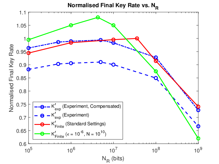
The optimal $N_{R}=3.6\times 10^{7}$ and $5\times 10^{6}$ are found for $K_{Finite}^{\prime}$ and $K_{exp}^{\prime}$, respectively. Assuming the usual practical scheme where $N_{R}$ is simply selected randomly, our results for the standard CV-QKD settings show that using the optimal $N_{R}$ for SR leads to a maximum gain of $33\%$ on the final key rate. Other CV-QKD settings will provide different maximum gains. For example, the green curve of Fig. 6 provides for a $66\%$ gain (not shown in the figure are the rates for $N_{R}>10^{9}$). This point emphasises the need to consider the parameter settings before determining both the optimal $N_{R}$ and the gain achieved relative to the standard practice of simply picking some $N_{R}<N$. Note that in our rate determinations, the normalisation of one in Fig. 6 corresponds to a key rate $K_{Finite}^{\prime}=4.3\times 10^{5}$ bits per second, based on our hardware-specific value of $c_{h}=3.2\times 10^{-9}$ seconds.¹⁶¹⁶ 16 We adopted the following method to determine $c_{h}$. For $m$ LDPC codes with $N_{R}=10^{6}$ and $T=0.9$, we obtained the total number of arithmetic operations for those codes. Next, we measured the elapsed time to reconcile a block of $10^{6}$ quadrature values. We then obtained $c_{h}$ by dividing the number of arithmetic operations to this measured elapsed time. The reconciliation rate associated with this same key rate is $3.9\times 10^{6}$ bits per second. Assuming the source rate of the quantum signalling was high enough (e.g. a 100MHz source), this reconciliation rate is higher than that required for delivery of secured ($\epsilon=10^{-9}$) keys ($N=10^{9}$) within flyover times (270 seconds) consistent with Micius-type orbits (see the introduction).

Comparing the two curves in Fig. 6, we find that there is still a small discrepancy between $K_{Finite}^{\prime}$ and $K_{exp}^{\prime}$ although they share a similar trend. The reason for such discrepancy is twofold. Firstly, there remain small trapping sets in the LDPC matrices.¹⁷¹⁷ 17 These trapping sets are the primary reason that additional decoding iterations are consumed for only a marginal decrease of the decoding error, i.e. the error floor effect[58]. Although not part of our analysis (but included in the uncompensated curve of Fig. 6), we attempted to remove these trapping sets in our codes by using the algorithm of [58] so that fewer iterations will be used [59]. This reduced the number of decoding iterations by approximately $15\%$ for $N_{R}=10^{6}$ but did not remove the trapping sets completely. The remnant trapping sets inside the LDPC matrices lead to a larger number of decoding iterations than predicted by $D_{j}$. Determined by the Density Evolution Algorithm, $D_{j}$ is a lower bound due to the assumption of cycle-free matrices and infinitely long block length[60]. Secondly, we note that selecting $R_{j}$ so that $\sum_{j=0}^{m-1}R_{j}$ achieves $C_{Finite}$ may lead to a $p_{Decode}$ higher than the given $\epsilon_{EC}$. In our experiment (and included in the shown results), we find that the $K_{exp}^{\prime}$ is $9\%$ lower than the $K_{Finite}^{\prime}$ predicted by Eq. 22 due to the gap between $\sum_{j=0}^{m-1}R_{j}$ and $C_{Finite}$.

In the satellite-based scenario, Alice and Bob starts the protocol with only $N_{o}$ quantum signals because the satellite is only visible to the ground station for a limited time frame. In this section, we revisit the analysis of the final key rate in the finite-key regime and conduct a numerical search to show how the final key rate $K$ is affected by $N_{e}$, for a given $N_{o}$ and $\epsilon$.

In Fig. 7, we observe that $K$ is cut off when $N_{e}$ approaches $10^{7}$ and $10^{9}$ (for $N_{o}=10^{9}$). At $N_{e}=10^{7}$, the parameter confidence intervals are not consistent with a positive $K$. As $N_{e}$ approaches $N_{o}$, $K$ decreases rapidly since the number of quantum signals for reconciliation approaches zero. Similar remarks can also be applied for $N_{o}=10^{10}$. In Fig. 7, we see that setting $N_{e}=\frac{N_{o}}{2}$ is an acceptable compromise between accommodating finite-key effects and preserving enough quantum signals for the post-processing. In the appendix, we investigate varying $N_{e}$ but where it is always constrained to $N_{e}=\frac{N_{o}}{2}$.

References

- [1] N. Hosseinidehaj, Z. Babar, R. Malaney, S. X. Ng, and L. Hanzo, “Satellite-Based Continuous-Variable Quantum Communications: State-of-the-Art and a Predictive Outlook,” IEEE Communications Surveys & Tutorials, vol. 21, no. 1, 881–919, 2018.
- [2] C. H. Bennett and G. Brassard, “Quantum Cryptography: Public Key Distribution and Coin Tossing,” in Proceedings of IEEE International Conference on Computers, Systems and Signal Processing,, vol. 175, 8, 1984.
- [3] H. Weinfurter, “Quantum Communication Experiments with Discrete Variables,” Quantum Information: From Foundations to Quantum Technology Applications, 369–381, 2016.
- [4] L. Gyöngyösi, L. Bacsardi, and S. Imre, “A Survey on Quantum Key Distribution,” Infocommunications Journal, vol. 11, no. 2, 14–21, 2019.
- [5] S. Pirandola, U. L. Andersen, L. Banchi, M. Berta, D. Bunandar, R. Colbeck, D. Englund, T. Gehring, C. Lupo, C. Ottaviani, et al., “Advances in Quantum Cryptography,” Advances in Optics and Photonics, vol. 12, no. 4, 1012–1236, 2020.
- [6] B. Korzh, C. C. W. Lim, R. Houlmann, N. Gisin, M. J. Li, D. Nolan, B. Sanguinetti, R. Thew, and H. Zbinden, “Provably Secure and Practical Quantum Key Distribution over 307 km of Optical Fibre,” Nature Photonics, vol. 9, no. 3, 163–168, 2015.
- [7] T. A. Eriksson, T. Hirano, B. J. Puttnam, G. Rademacher, R. S. Luís, M. Fujiwara, R. Namiki, Y. Awaji, M. Takeoka, N. Wada, et al., “Wavelength Division Multiplexing of Continuous Variable Quantum Key Distribution and 18.3 Tbit/s Data Channels,” Communications Physics, vol. 2, no. 1, 1–8, 2019.
- [8] S.-Y. Shen, M.-W. Dai, X.-T. Zheng, Q.-Y. Sun, G.-C. Guo, and Z.-F. Han, “Free-Space Continuous-Variable Quantum Key Distribution of Unidimensional Gaussian Modulation Using Polarized Coherent States in an Urban Environment,” Physical Review A, vol. 100, 012325, 2019.
- [9] L. Gyongyosi and S. Imre, “Secret Key Rates of Free-Space Optical Continuous-Variable Quantum Key Distribution,” International Journal of Communication Systems, vol. 32, no. 18, e4152, 2019.
- [10] P. Jouguet, S. Kunz-Jacques, and A. Leverrier, “Long-Distance Continuous-Variable Quantum Key Distribution with a Gaussian Modulation,” Physical Review A, vol. 84, no. 6, 062317, 2011.
- [11] P. Jouguet, S. Kunz-Jacques, T. Debuisschert, S. Fossier, E. Diamanti, R. Alléaume, R. Tualle-Brouri, P. Grangier, A. Leverrier, P. Pache, et al., “Field Test of Classical Symmetric Encryption with Continuous Variables Quantum Key Distribution,” Optics Express, vol. 20, no. 13, 14030–14041, 2012.
- [12] Q. Liao, Y. Guo, D. Huang, P. Huang, and G. Zeng, “Long-Distance Continuous-Variable Quantum Key Distribution Using Non-Gaussian State-Discrimination Detection,” New Journal of Physics, vol. 20, no. 2, 023015, 2018.
- [13] D. Guo, C. He, T. Guo, Z. Xue, Q. Feng, and J. Mu, “Comprehensive High-Speed Reconciliation for Continuous-Variable Quantum Key Distribution,” Quantum Information Processing, vol. 19, no. 9, 1–19, 2020.
- [14] Y. Zhang, Z. Chen, S. Pirandola, X. Wang, C. Zhou, B. Chu, Y. Zhao, B. Xu, S. Yu, and H. Guo, “Long-Distance Continuous-Variable Quantum Key Distribution over 202.81 km of Fiber,” Physical Review Letters, vol. 125, no. 1, 010502, 2020.
- [15] A. Leverrier, F. Grosshans, and P. Grangier, “Finite-Size Analysis of a Continuous-Variable Quantum Key Distribution,” Physical Review A, vol. 81, no. 6, 062343, 2010.
- [16] F. Furrer, T. Franz, M. Berta, A. Leverrier, V. B. Scholz, M. Tomamichel, and R. F. Werner, “Continuous Variable Quantum Key Distribution: Finite-Key Analysis of Composable Security against Coherent Attacks,” Physical Review Letters, vol. 109, no. 10, 100502, 2012.
- [17] S. Kish, E. Villaseñor, R. Malaney, K. Mudge, and K. Grant, “Feasibility Assessment for Practical Continuous Variable Quantum Key Distribution over the Satellite-to-Earth Channel,” Quantum Engineering, vol. 2, no. 3, e50, 2020.
- [18] M. Tomamichel, C. C. W. Lim, N. Gisin, and R. Renner, “Tight Finite-Key Analysis for Quantum Cryptography,” Nature Communications, vol. 3, no. 1, 1–6, 2012.
- [19] Z. Yuan, A. Plews, R. Takahashi, K. Doi, W. Tam, A. Sharpe, A. Dixon, E. Lavelle, J. Dynes, A. Murakami, et al., “10-Mb/s Quantum Key Distribution,” Journal of Lightwave Technology, vol. 36, no. 16, 3427–3433, 2018.
- [20] S.-K. Liao, W.-Q. Cai, W.-Y. Liu, L. Zhang, Y. Li, J.-G. Ren, J. Yin, Q. Shen, Y. Cao, Z.-P. Li, et al., “Satellite-to-Ground Quantum Key Distribution,” Nature, vol. 549, no. 7670, 43–47, 2017.
- [21] D. Lin, D. Huang, P. Huang, J. Peng, and G. Zeng, “High Performance Reconciliation for Continuous-Variable Quantum Key Distribution with LDPC Code,” International Journal of Quantum Information, vol. 13, no. 02, 1550010, 2015.
- [22] X. Wang, Y. Zhang, S. Yu, B. Xu, Z. Li, and H. Guo, “Efficient Rate-Adaptive Reconciliation for Continuous-Variable Quantum Key Distribution,” Quantum Information & Computation, vol. 17, no. 13–14, 1123–1134, 2017.
- [23] C. Zhou, X. Wang, Y. Zhang, Z. Zhang, S. Yu, and H. Guo, “Continuous-Variable Quantum Key Distribution with Rateless Reconciliation Protocol,” Physical Review Applied, vol. 12, no. 5, 054013, 2019.
- [24] M. Milicevic, C. Feng, L. M. Zhang, and P. G. Gulak, “Quasi-Cyclic Multi-Edge LDPC Codes for Long-Distance Quantum Cryptography,” NPJ Quantum Information, vol. 4, no. 1, 1–9, 2018.
- [25] S.-S. Yang, Z.-G. Lu, and Y.-M. Li, “High-Speed Post-Processing in Continuous-Variable Quantum Key Distribution Based on FPGA Implementation,” Journal of Lightwave Technology, vol. 38, no. 15, 3935–3941, 2020.
- [26] H. Li and Y. Pang, “FPGA-Accelerated Quantum Computing Emulation and Quantum Key Distillation,” IEEE Micro, vol. 41, no. 4, 49–57, 2021.
- [27] C. Weedbrook, A. M. Lance, W. P. Bowen, T. Symul, T. C. Ralph, and P. K. Lam, “Quantum Cryptography without Switching,” Physical Review Letters, vol. 93, no. 17, 170504, 2004.
- [28] N. Hosseinidehaj, A. M. Lance, T. Symul, N. Walk, and T. C. Ralph, “Finite-Size Effects in Continuous-Variable Quantum Key Distribution with Gaussian Postselection,” Physical Review A, vol. 101, no. 5, 052335, 2020.
- [29] D. Dequal, L. T. Vidarte, V. R. Rodriguez, G. Vallone, P. Villoresi, A. Leverrier, and E. Diamanti, “Feasibility of Satellite-to-Ground Continuous-Variable Quantum Key Distribution,” NPJ Quantum Information, vol. 7, no. 1, 1–10, 2020.
- [30] M. Bloch, A. Thangaraj, and S. W. McLaughlin, “Efficient Reconciliation of Correlated Continuous Random Variables Using LDPC Codes,” arXiv preprint cs/0509041, 2005.
- [31] P. Jouguet, D. Elkouss, and S. Kunz-Jacques, “High-Bit-Rate Continuous-Variable Quantum Key Distribution,” Physical Review A, vol. 90, no. 4, 042329, 2014.
- [32] H. Mani, T. Gehring, P. Grabenweger, B. Ömer, C. Pacher, and U. L. Andersen, “Multiedge-Type Low-Density Parity-Check Codes for Continuous-Variable Quantum Key Distribution,” Physical Review A, vol. 103, no. 6, 062419, 2021.
- [33] H. Imai and S. Hirakawa, “A New Multilevel Coding Method Using Error-Correcting Codes,” IEEE Transactions on Information Theory, vol. 23, no. 3, 371–377, 1977.
- [34] U. Wachsmann, R. F. Fischer, and J. B. Huber, “Multilevel codes: Theoretical concepts and practical design rules,” IEEE Transactions on Information Theory, vol. 45, no. 5, 1361–1391, 1999.
- [35] R. D. Wesel, X. Liu, J. M. Cioffi, and C. Komninakis, “Constellation Labeling for Linear Encoders,” IEEE Transactions on Information Theory, vol. 47, no. 6, 2417–2431, 2001.
- [36] M. Bloch, A. Thangaraj, S. W. McLaughlin, and J.-M. Merolla, “LDPC-Based Gaussian Key Reconciliation,” in IEEE Information Theory Workshop-ITW’06 Punta del Este, 116–120, IEEE, 2006.
- [37] A. Leverrier, R. Alléaume, J. Boutros, G. Zémor, and P. Grangier, “Multidimensional Reconciliation for a Continuous-Variable Quantum Key Distribution,” Physical Review A, vol. 77, no. 4, 042325, 2008.
- [38] J. Fiurášek and N. J. Cerf, “Gaussian Postselection and Virtual Noiseless Amplification in Continuous-Variable Quantum Key Distribution,” Physical Review A, vol. 86, no. 6, 060302, 2012.
- [39] F. Darema, “The SPMD Model: Past, Present and Future,” in European Parallel Virtual Machine/Message Passing Interface Users’ Group Meeting, 1–1, Springer, 2001.
- [40] M. Pharr and W. R. Mark, “A SPMD Compiler for High-Performance CPU Programming,” in Innovative Parallel Computing (InPar), 1–13, IEEE, 2012.
- [41] J. Lodewyck, M. Bloch, R. García-Patrón, S. Fossier, E. Karpov, E. Diamanti, T. Debuisschert, N. J. Cerf, R. Tualle-Brouri, S. W. McLaughlin, et al., “Quantum Key Distribution over 25 km with an All-Fiber Continuous-Variable System,” Physical Review A, vol. 76, no. 4, 042305, 2007.
- [42] F. Laudenbach, C. Pacher, C.-H. F. Fung, A. Poppe, M. Peev, B. Schrenk, M. Hentschel, P. Walther, and H. Hübel, “Continuous-Variable Quantum Key Distribution with Gaussian Modulation—The Theory of Practical Implementations,” Advanced Quantum Technologies, vol. 1, no. 1, 1800011, 2018.
- [43] Y. Polyanskiy, H. V. Poor, and S. Verdú, “Channel Coding Rate in the Finite Blocklength Regime,” IEEE Transactions on Information Theory, vol. 56, no. 5, 2307–2359, 2010.
- [44] D. Slepian and J. Wolf, “Noiseless Coding of Correlated Information Sources,” IEEE Transactions on Information Theory, vol. 19, no. 4, 471–480, 1973.
- [45] T. Richardson and R. Urbanke, Modern Coding Theory. Cambridge University Press, 2008.
- [46] X. Ai, R. Malaney, and S. X. Ng, “A Reconciliation Strategy for Real-Time Satellite-Based QKD,” IEEE Communications Letters, vol. 24, no. 5, 1062–1066, 2020.
- [47] S.-Y. Chung, T. J. Richardson, and R. L. Urbanke, “Analysis of Sum-Product Decoding of Low-Density Parity-Check Codes Using a Gaussian Approximation,” IEEE Transactions on Information Theory, vol. 47, no. 2, 657–670, 2001.
- [48] V. A. Chandrasetty and S. M. Aziz, “FPGA Implementation of an LDPC Decoder Using a Reduced Complexity Message Passing Algorithm,” Journal of Networks, vol. 6, no. 1, 36, 2011.
- [49] A. Leverrier, “Composable Security Proof for Continuous-Variable Quantum Key Distribution with Coherent States,” Physical Review Letters, vol. 114, no. 7, 070501, 2015.
- [50] C. Lupo, C. Ottaviani, P. Papanastasiou, and S. Pirandola, “Continuous-Variable Measurement-Device-Independent Quantum Key Distribution: Composable Security against Coherent Attacks,” Physical Review A, vol. 97, no. 5, 052327, 2018.
- [51] N. Hosseinidehaj, N. Walk, and T. C. Ralph, “Optimal Realistic Attacks in Continuous-Variable Quantum Key Distribution,” Physical Review A, vol. 99, no. 5, 052336, 2019.
- [52] S. Pirandola, “Limits and Security of Free-Space Quantum Communications,” Physical Review Research, vol. 3, no. 1, 013279, 2021.
- [53] S. Pirandola, “Satellite Quantum Communications: Fundamental Bounds and Practical Security,” Physical Review Research, vol. 3, no. 2, 023130, 2021.
- [54] J. H. Mathews and K. D. Fink, Numerical Methods Using MATLAB, vol. 4. Pearson Prentice Hall Upper Saddle River, NJ, 2004.
- [55] A. Leverrier, “Security of Continuous-Variable Quantum Key Distribution via a Gaussian de Finetti Reduction,” Physical Review Letters, vol. 118, no. 20, 200501, 2017.
- [56] E. Villaseñor, R. Malaney, K. A. Mudge, and K. J. Grant, “Atmospheric Effects on Satellite-to-Ground Quantum Key Distribution Using Coherent States,” in GLOBECOM 2020-2020 IEEE Global Communications Conference, 1–6, IEEE, 2020.
- [57] J. Mateo, Efficient Information Reconciliation for Quantum Key Distribution. PhD thesis, Universidad Politecnica de Madrid, 2011.
- [58] T. Tian, C. R. Jones, J. D. Villasenor, and R. D. Wesel, “Selective Avoidance of Cycles in Irregular LDPC Code Construction,” IEEE Transactions on Communications, vol. 52, no. 8, 1242–1247, 2004.
- [59] D. V. Nguyen, S. K. Chilappagari, M. W. Marcellin, and B. Vasic, “On the Construction of Structured LDPC Codes Free of Small Trapping Sets,” IEEE Transactions on Information Theory, vol. 58, no. 4, 2280–2302, 2012.
- [60] S. Landner and O. Milenkovic, “Algorithmic and Combinatorial Analysis of Trapping Sets in Structured LDPC Codes,” in International Conference on Wireless Networks, Communications and Mobile Computing, vol. 1, 630–635, IEEE, 2005.
- [61] X. Wang, Y. Zhang, S. Yu, and H. Guo, “High Speed Error Correction for Continuous-Variable Quantum Key Distribution with Multi-Edge Type LDPC Code,” Scientific Reports, vol. 8, no. 1, 1–7, 2018.
- [62] Y. Li, X. Zhang, Y. Li, B. Xu, L. Ma, J. Yang, and W. Huang, “High-Throughput GPU Layered Decoder of Quasi-Cyclic Multi-Edge Type Low Density Parity Check Codes in Continuous-Variable Quantum Key Distribution Systems,” Scientific Reports, vol. 10, no. 1, 1–11, 2020.
- [63] F. Grosshans, “Collective Attacks and Unconditional Security in Continuous Variable Quantum Key Distribution,” Physical Review Letters, vol. 94, 020504, 2005.
- [64] M. Navascués, F. Grosshans, and A. Acin, “Optimality of Gaussian Attacks in Continuous-Variable Quantum Cryptography,” Physical Review Letters, vol. 97, no. 19, 190502, 2006.
- [65] S. Fossier, E. Diamanti, T. Debuisschert, R. Tualle-Brouri, and P. Grangier, “Improvement of Continuous-Variable Quantum Key Distribution Systems by Using Optical Preamplifiers,” Journal of Physics B: Atomic, Molecular and Optical Physics, vol. 42, no. 11, 114014, 2009.
- [66] P. Jouguet, S. Kunz-Jacques, E. Diamanti, and A. Leverrier, “Analysis of Imperfections in Practical Continuous-Variable Quantum Key Distribution,” Physical Review A, vol. 86, no. 3, 032309, 2012.
In this appendix, we elaborate on the estimation of channel parameters, and , from quantum signals and determination of the upper bound of based on the estimated and for a given . Here, we closely follow the methodology in [17] (and references therein).
The parameter estimation at Step 4 of our protocol is a two-step process. Firstly, Alice and Bob estimate each coefficient in the covariance matrix between the shared states based on (randomly selected) quantum signals sent from Bob. Then Alice uses these estimated coefficients to determine and . In the asymptotic regime, the estimation of and is exact since Alice and Bob use an infinite number of quantum signals. The following the two functions will be useful,