Combating Informational Denial-of-Service (IDoS) Attacks: Modeling and Mitigation of Attentional Human Vulnerability

We summarize notations in Table 1. The rest of the paper is organized as follows. Section 2 introduces the system modeling for IDoS attacks, alert generations, and the inspections of human operators. Based on the system model, we present a Semi-Markov Process (SMP) model in Section 3 to evaluate human performance, the severity level, and the risks of IDoS attacks. We present a case study in Section 4 to corroborate our results and Section 5 concludes the paper.

As shown in Fig. 2, there is an analogy between the Denial-of-Service (DoS) attacks in communication networks and the Informational Denial-of-Service (IDoS) attacks in the human-in-the-loop systems. Both of them achieve their attack goals by exhausting the limited resources. DoS attacks happen when the attacker generates a large number of superfluous requests to deplete the computing resource of the targeted machine and prevent the fulfillment of legitimate services. Analogously, IDoS attacks create a large amount of unprocessed information to deplete cognitive resources of human operators and prevent them from acquiring the knowledge contained in the information.

We list several assailable cognitive resources under IDoS attacks as follows.

• •

  Attention: Paying sustained attention to acquire proper information is costly. From an economic perspective, inattention occurs when the cost of information acquisition is lower than the attention cost measured by the information entropy [11]. IDoS attacks generate feints to distract the human from the right information. An excessive number of feints prohibit the human from process any information.

• •

  Memory and Learning Capacity: Humans have limited memory and learning capacity. Humans cannot remember the details or learn new things if there is an information overload [2].

• •

  Reasoning: Human decision-making consumes a large amount of energy, which is one of the reasons why we have two modes of thought [12] (‘system $1$’ thinking is fast, instinctive, and emotional; while ‘system $2$’ thinking is slower and more logical). IDoS attacks can exert a heavy cognitive load to prevent humans from deliberative decisions that use the ‘system $2$’ thinking. Moreover, evidence shows the paradox of choice [13]; i.e., rich choices can bring anxiety and prevent humans from making any decisions.

When these cognitive resources are exhausted, the information cannot be processed correctly and timely and serves as noise that leads to alert fatigue [14]. We use operators in the control room of nuclear power plants as a stylized example to illustrate the consequences of IDoS attacks and motivate the need for the security technology to assist human operators against IDoS attacks.

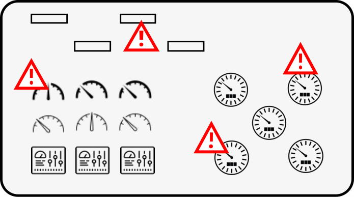
In Fig. 3, a monitor screen contains meters that show the real-time readings of the temperature, pressure, and flow rate in a nuclear power plant. Based on the pre-defined generation rules, warnings and messages pop up at different locations. Due to the complexity of the nuclear control system, the inspection of these alerts consumes the operator’s time and cognitive resources. The attempt to inspect all alerts and the constant switching among them can lead to missed detection and erroneous behaviors. If the alerts are generated strategically by attacks, they may further mislead humans to take actions in the attacker’s favor; e.g., focusing on feints and ignoring the real attacks that hide among feints.

One way to mitigate IDoS attacks is to train the operators or human users to deal with the information overload and remain vigilant and productive under a heavy cognitive load. However, attentional training can be time-consuming and the effectiveness is not guaranteed. The second method is to recruit more human operators to share the information load. It would require the coordination of the operator team and can incur additional costs of human resources. The third method is to develop assistive technologies to rank and filter the information to alleviate the cognitive load of human operators. It would leverage past experiences and data analytics to pinpoint and prioritize critical alerts for human operators to process. The first two methods aim to increase the capacity or the volume of the cognitive resources in Fig. 2. The third method pre-processes the information so that it adapts to the capacity and characteristics of cognitive resources.

In this work, we focus on the temporal aspect of the alerts (i.e., the frequency and duration of their arrivals). The future work will incorporate their spatial locations on the monitor screen as shown in Fig. 3. As highlighted by the orange background in Fig. 4, attacks arrive sequentially at time $t^{k},k\in\mathbb{Z}^{0+}$ where $t^{0}=0$. Let $\tau^{k}:=t^{k+1}-t^{k}\in[0,\infty)$ be the inter-arrival time between the $(k+1)$-th attack and the $k$-th attack for all $k\in\mathbb{Z}^{0+}$. We refer to the $k$-th attack equivalently as the one at attack stage $k\in\mathbb{Z}^{0+}$.

Each attack can be either a feint (denoted by $\theta_{FE}$) or a real attack (denoted by $\theta_{RE}$) with probability $b_{FE}\in[0,1]$ and $b_{RE}\in[0,1]$, respectively, where $b_{FE}+b_{RE}=1$. We assume that both types of attacks trigger alerts with the same time delay. Thus, there is a one-to-one mapping between the sequence of attacks and alerts, and we can consider the zero delay time without loss of generality. The alerts cannot reflect the attack’s type denoted by $\theta^{k}\in\Theta:=\{\theta_{FE},\theta_{RE}\}$ at all attack stages $k\in\mathbb{Z}^{0+}$. However, the alerts can provide human operators with a category label from a finite set $\mathcal{S}$ based on observable features or traces of the associated attacks, e.g., the attack locations as shown in Section 4. We denote the alert’s category label at attack stage $k\in\mathbb{Z}^{0+}$ as $s^{k}\in\mathcal{S}$.

Since an alert does not directly reflect whether the attack is feint or real, human operators need to inspect the alert to determine the hidden type, which leads to three security decisions: the attack is feint (denoted by $w_{FE}$), the attack is real (denoted by $w_{RE}$), or the attack’s type is unknown (denoted by $w_{UN}$). We use $w^{k}\in\mathcal{W}:=\{w_{FE},w_{RE},w_{UN}\}$ to denote the human operator’s security decision of the $k$-th alert. Each human operator has limited attention and cannot inspect multiple alerts simultaneously. Moreover, the human operator requires sustained attention on an alert to make an accurate security decision. Frequent alert pop-ups can distract humans from the current alert inspection and result in alert fatigue and the paradox of choice as illustrated in Section 2.1. To compensate for the human’s attention limitation, we can intentionally make some alerts less noticeable, e.g., without sounds or in a light color. Then, the human can pay sustained attention to the alert currently under inspection. These inconspicuous alerts can be assigned to other available inspectors with an additional cost of human resources. If these alerts are time-insensitive, they can also be queued and inspected later by the same operator at his convenience. However, in practice, the number of alerts usually far exceeds the number of available inspectors, and the alerts cannot tolerate delay. Then, these alerts are dismissed as a tradeoff for the timely and accurate inspection of the other highlighted alerts. In this case, these inconspicuous alerts are not inspected and automatically assigned the security decision $w_{UN}$.

In this paper, we focus on the class of Attention Management (AM) strategies, denoted by $\mathcal{A}:=\{a_{m}\}_{m\in\mathbb{Z}^{+}}$, that highlight alerts periodically to engage operators in the alert inspection. We assume that the human operator can only notice and inspect an alert when it is highlighted. Then, AM strategy $a_{m}\in\mathcal{A}$ means that the human operator inspects the alerts at attack stages $k=hm,h\in\mathbb{Z}^{0+}$. We refer to the attack stages during the $h$-th inspection as the inspection stage $h\in\mathbb{Z}^{0+}$. Then, under AM strategy $a_{m}\in\mathcal{A}$, each inspection stage contains $m$ attack stages as shown in the blue background of Fig. 4. The $h$-th inspection has a duration of $\tau_{IN}^{h,m}:=\sum_{{k}^{\prime}=hm}^{hm+m-1}\tau^{{k}^{\prime}}$ for all $h\in\mathbb{Z}^{0+}$.

Since the inspection is made every $m$ attack stages, we define the consolidated state $x^{h}:=[s^{hm},\cdots,s^{hm+m-1}]\in\mathcal{X}:=\mathcal{S}^{m}$ that consists of the category labels of $m$ successive alerts at inspection stage $h\in\mathbb{Z}^{0+}$. Analogously, we define the consolidated type $\bar{\theta}^{h}:=[\theta^{hm},\cdots,\theta^{hm+m-1}]\in\bar{\Theta}:=\Theta^{m}$. Then, we denote the transition function of the consolidated state as $\bTr(x^{h+1}|x^{h};\bar{\theta}^{h})$, which is also Markov as shown below.

The inspection time $\tau_{IN}^{h,m}=\sum_{{k}^{\prime}=hm}^{hm+m-1}\tau^{{k}^{\prime}}$ at inspection stage $h\in\mathbb{Z}^{0+}$ is a continuous random variable with support $[0,\infty)$ whose PDF $\bar{z}(\cdot|x^{h};\bar{\theta}^{h})$ can be computed based on the PDF $z$. Based on $\bar{z}$ and $\Pr(w^{hm}|s^{hm},\tau_{IN}^{h,m};\theta^{hm})$ in (1) and (2), we can compute the probability of security decision $w^{hm}$ at inspection stage $h\in\mathbb{Z}^{0+}$ given $x^{h}$ and $\bar{\theta}^{h}$, i.e.,

Let ${\Pr}(w^{hm}|x^{h},a_{m};{\theta}^{hm})$ be the shorthand notation for $\mathbb{E}_{\theta^{l}\sim[b_{FE},b_{RE}],l\in\{hm+1,\cdots,hm+m-1\}}\allowbreak[\Pr(w^{hm}|x^{h},a_{m};\bar{\theta}^{h})],\forall\theta^{hm}\in\Theta$. We define the probability of the human operator making correct security decisions at inspection stage $h\in\mathbb{Z}^{0+}$ as

which leads to the consolidated severity level of IDoS attacks in Definition 1.

We denote $c(w^{k},s^{k};\theta^{k})$ as the operator’s cost at attack stage $k\in\mathbb{Z}^{0+}$ when the alert’s category label is $s^{k}\in\mathcal{S}$, the attack’s type is $\theta^{k}\in\Theta$, and the security decision is $w^{k}\in\mathcal{W}$. At attack stages where alerts are inconspicuous, i.e., for all $k\neq hm,h\in\mathbb{Z}^{0+}$, the security decision is $w_{UN}$ without manual inspection, which incurs an uncertainty cost $c_{UN}>0$. At attack stages of highlighted alerts, i.e., for all $k=hm,h\in\mathbb{Z}^{0+}$, the human operator obtains a reward (resp. cost), denoted by $c_{CD}(s^{k};\theta^{k})<0$ (resp. $c_{ID}(s^{k};\theta^{k})>0$), for correct (resp. incorrect) security decisions. If the human operator remains uncertain about the attack’s type after the inspection time $\tau_{IN}^{h,m}$, i.e., $w^{hm}=w_{UN}$, there is the uncertainty cost $c_{UN}$. We define the human operator’s consolidated cost at inspection stage $h\in\mathbb{Z}^{0+}$ as

In this section, we define four long-term risk measures whose relations are shown in Fig. 6. The Cumulative Cost (CC) and Expected Cumulative Cost (ECC) on the left directly follow from the discounted summation of the consolidated cost $\bar{c}$ in (6). Since CC and ECC depend on the consolidated state $x^{h}$ and the consolidated type $\bar{\theta}^{h}$, it is of high dimension and thus difficult to store and compute. By taking an expectation over $s^{hm+1},\cdots,s^{hm+m-1}\in\mathcal{S}$, we reduce the dimension and obtain the Aggregated Cumulative Cost (ACC) and Expected Aggregated Cumulative Cost (EACC) on the right of the figure. The DP representations for CC (resp. ECC) and ACC (resp. EACC) are generally not equivalent. We identify the condition under which two DP representations are equivalent in Section 3.3. The two risk learning schemes are introduced in Section 3.4. Since the consolidated risk learning is based on ECC, it has to wait for the realization of the consolidated state $x^{h}:=[s^{hm},\cdots,s^{hm+m-1}]$ to evaluate the inspection performance. On the contrary, the EACC-based aggregated risk learning just needs $s^{hm}$ to evaluate the inspection performance, which reduces the dimension of the samples and enables evaluations with no delay.

In Section 3.3, we consider the special case where PDF $z$ is independent of $s^{k}$ and $\theta^{k}$, which reduces the dependency of $\hat{p}_{CD}$ and $\bar{c}$ from $x^{h}$ to $s^{hm}$ as shown in Lemma 2. Moreover, we can obtain DP representations for ACC $\tilde{u}$ and EACC $\bar{u}$ as shown in Theorem 3.1. Value iteration in Algorithm 1 can be revised accordingly to solve these two DP representations.

References

- [1] B. Hitzel. (2019) The art of cyber war and cyber battle: Deception operations. https://www.networkdefenseblog.com/post/art-of-cyber-war-deception.
- [2] C. D. Wickens, J. G. Hollands, S. Banbury, and R. Parasuraman, Engineering psychology and human performance. Psychology Press, 2015.
- [3] W. Casey, J. A. Morales, E. Wright, Q. Zhu, and B. Mishra, “Compliance signaling games: toward modeling the deterrence of insider threats,” Computational and Mathematical Organization Theory, vol. 22, no. 3, pp. 318–349, 2016.
- [4] L. Huang and Q. Zhu, “Duplicity games for deception design with an application to insider threat mitigation,” IEEE Transactions on Information Forensics and Security, 2021.
- [5] ——, “Inadvert: An interactive and adaptive counterdeception platform for attention enhancement and phishing prevention,” arXiv preprint arXiv:2106.06907, 2021.
- [6] Y. Huang, L. Huang, and Q. Zhu, “Reinforcement learning for feedback-enabled cyber resilience,” arXiv preprint arXiv:2107.00783, 2021.
- [7] L. Huang and Q. Zhu, “A dynamic games approach to proactive defense strategies against advanced persistent threats in cyber-physical systems,” Computers & Security, vol. 89, p. 101660, 2020.
- [8] ——, “A dynamic game framework for rational and persistent robot deception with an application to deceptive pursuit-evasion,” IEEE Transactions on Automation Science and Engineering, pp. 1–15, 2021.
- [9] ——, “Adaptive honeypot engagement through reinforcement learning of semi-markov decision processes,” in International Conference on Decision and Game Theory for Security. Springer, 2019, pp. 196–216.
- [10] D. Zhao, J. Liu, J. Wang, W. Niu, E. Tong, T. Chen, and G. Li, “Bidirectional rnn-based few-shot training for detecting multi-stage attack,” arXiv preprint arXiv:1905.03454, 2019.
- [11] C. A. Sims, “Implications of rational inattention,” Journal of monetary Economics, vol. 50, no. 3, pp. 665–690, 2003.
- [12] D. Kahneman, Thinking, fast and slow. Macmillan, 2011.
- [13] B. Schwartz, “The paradox of choice: Why more is less.” Ecco New York, 2004.
- [14] T. Ban, N. Samuel, T. Takahashi, and D. Inoue, “Combat security alert fatigue with ai-assisted techniques,” in Cyber Security Experimentation and Test Workshop, 2021, pp. 9–16.
- [15] D. Bertsekas and J. Tsitsiklis, Neuro-Dynamic Programming, 01 1996, vol. 27.