Further insights into the mysteries of the values of zeta functions at integersThanks: J.M. is partially supported by the Natural Sciences and Engineering Research Council of Canada (NSERC) grant R0370A01. He gratefully acknowledges the Western University Faculty of Science Distinguished Professorship in 2020-2021 and support of Western Academy for Advanced Research as Western Fellow. N.D.T. is partially supported by the Ministry of Education and Training of Vietnam via the project ”On the arithmetic of algebraic groups and homogeneous spaces over local and global fields and their extensions”
Abstract.
We present a remarkably simple and surprisingly natural interpretation of the values of zeta functions at negative integers and zero. Namely we are able to relate these values to areas related to partial sums of powers. We apply these results to further interpretations of values of -functions at negative integers. We hint in a very brief way at some expected connections of this work with other current efforts to understand the mysteries of the values of zeta functions at integers.
Key words and phrases:
Hurwitz zeta functions, Bernoulli polynomials, Generalized Bernoulli numbers, -functions2010 Mathematics Subject Classification
Primary 11M35, 11M06, 11B68To the memory of Goro Shimura with gratitude and admiration
1. Introduction
Ever since Euler made stunning discoveries connecting some values of zeta functions with powers of , there has been a tremendous effort of mathematicians to comprehend well the “true reasons behind these connections” and to further extend these results to other values and other zeta functions. This work belongs to one of the most dramatic and exciting parts of mathematics and some parts of theoretical physics. Some extraordinary progress, conjectures, and various deep concepts have been obtained. Yet, the air of tremendous mystery, excitement, and strong desire to make further progress has never been altered nor slowed down.
Let us begin with two very naive questions which a child might ask:
- (1)
How many natural numbers are there?
- (2)
What is the sum of all natural numbers?
The obvious answers to both questions namely: “infinity” are correct but they lack a certain depth, subtlety, and connections with combinatorial properties of natural numbers. L. Euler was able to offer some more subtle and more interesting answers:
- (1)
- (2)
One has to be cautious when handling these beautiful Euler’s equalities in a formal way. As we shall see below that equalities can be explained in a subtle way as values of Rieman’s zeta function. However, in order to do it properly, the Riemann zeta function defined below as a convergent series for complex values for has to be analytically extended to the entire complex plane except when . Therefore one can not formally handle the equalities and in the usual way as when we consider just finite sums. For example if we just add formally both equalities we shall obtain equality:
However if we just subtract from the equation the number one we obtain
which would contradict the first equality.
Therefore below we consider rigorous proper modern interpretation of Euler’s equalities using values of Riemann zeta function.
We now write the above-mentioned equalities of Euler using the values of the Riemann zeta function as:
- (1)
- (2)
In fact, S. Ramanujan rediscovered these statements and for example formula appeared in exactly the same form in Ramanujan’s letter to G. Hardy addressed in 16 January, 1913 (see [1, page 351]).
Recall that the Riemann zeta function with is the analytical continuation of the function
with to the whole complex plane except when where has a simple pole (see [40]). Euler’s answers are deep and the assigned numbers as a summation of these divergent series have various interesting interpretations. For interested readers, we just refer to some articles and surveys related to these topics (see for examples [14], [18], [22], [25], [26], [29], [32]).
In paper [30], Mináč raised and answered the following naive question:
Question 1.1.
Suppose or . Are there any connections between the values and the partial sums
Here is considered as a polynomial in .
The answer is the fact on page 1 in [30]
Hence it is observed that
Thus is equal to times the area of the right triangle with acute angles and legs of length . This is because the graph of over the interval has the shape of a right triangle when taken together with the x-axis and y-axis (see the displayed Figure 1 below).
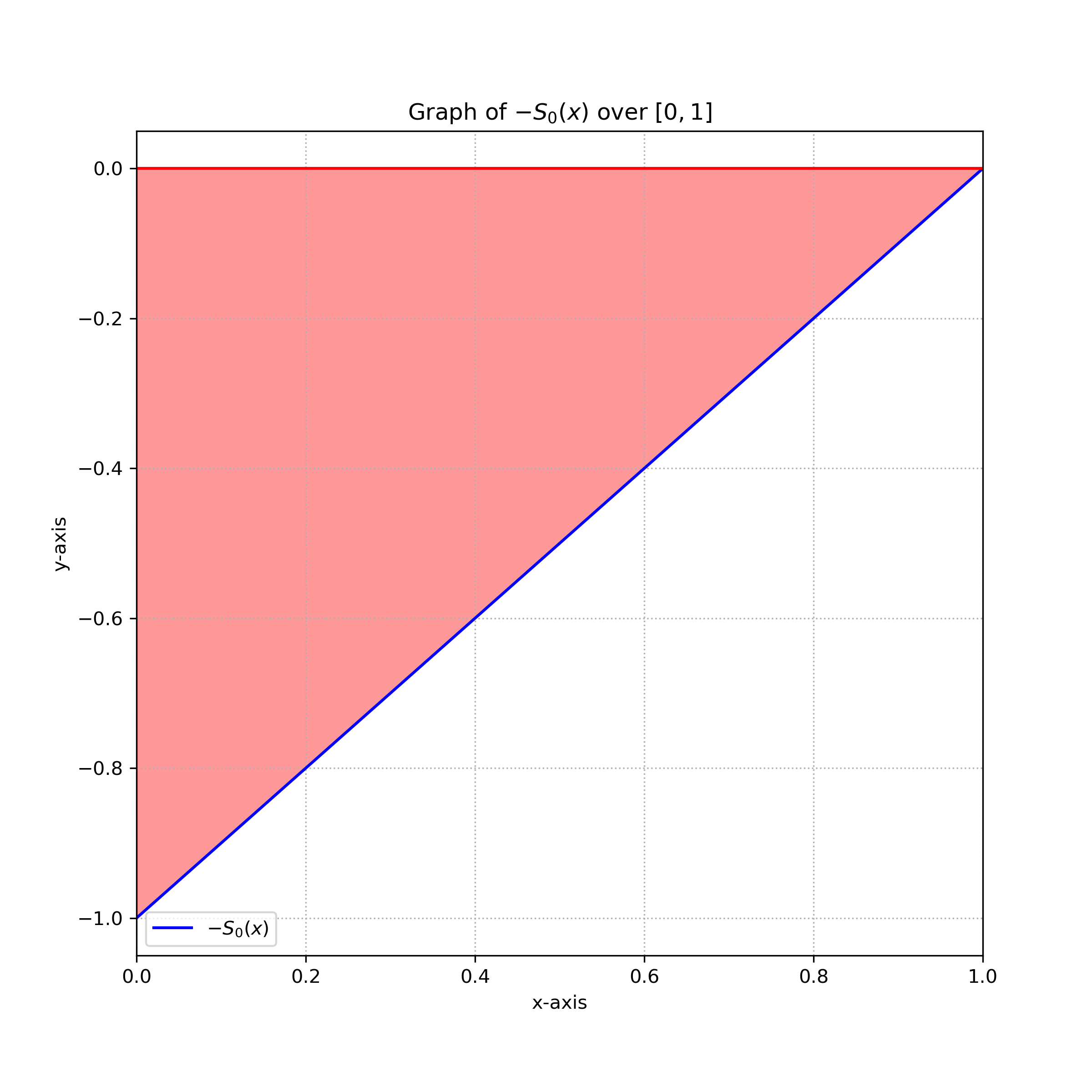
Similarly is time area of the red region in figure 2 below.

Observe also that
This fact also has a geometrical meaning as if
then
In fact, the graph displayed function of in the interval in figure , the red region bounded by the horizontal axis and , the blue region bounded by the horizontal axis and show that in the evaluation of the integral , the two areas considered with proper signs will cancel each other.
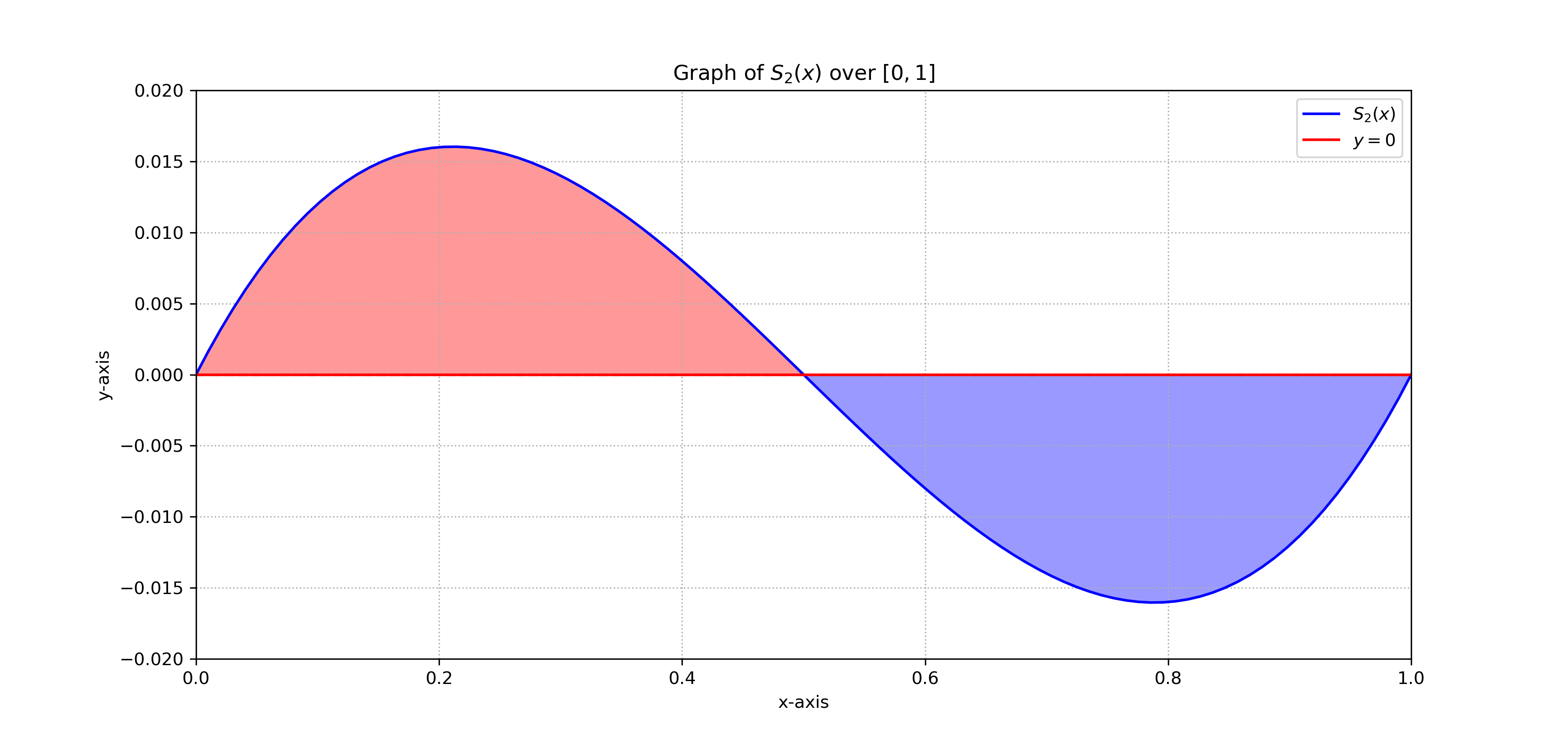
In fact, in general for all
where is the -th Bernoulli polynomial (see [33, Section 2, Chapter 1]). Hence if and , we see that
From the general property
we see immediately in general, in the evaluation
we obtain the cancellation of two signed areas as in the special case with . Hence we see a nice geometric explanation for all .
Because does not change sign between and (see [33, Section 3, Chapter 1]), we also see that all values are in fact signed areas of regions by the horizontal axis and functions These values are also equal to where are just Bernoulli numbers whose signs alternate.
Interested readers are encouraged to also see articles [39], [17]. This paper is meant as the first paper of a series of papers related to special values of -functions. It is beyond the scope of this paper to provide a comprehensive historical overview of the study of the special values of -functions and their arithmetic significance. Therefore, we merely point out several highlights of these investigations which also motivate our investigations. Some of these investigations are rather sophisticated and they involve the most advanced topics of current number theory. We hope that our elementary point of view and possibly unexpected direct connections with partial sums and signed areas will bring additional insight and inspiration to understand special values of -functions. We also hope to find a bridge between these elementary and more sophisticated studies of -functions in the subsequent papers.
One of the strongest motivations for studying special values of -functions is the class number formula for residue of the Dedekind zeta function of an algebraic number field expressed via basic invariants of like the regulator , the class number , the number of roots of unity contained in , discriminant , the number of real places , and the number of complex places . This remarkable formula has the following form
See for example [9, Chapter 5, Section 2.1]. This formula provides a bridge between the algebraic and the analytic world.
Observe in particular that . Because we see that the class number formula in view of amounts to and we recover the unique factorization of integers into products of primes. In fact, these strong immediate connections between arithmetic and analysis were already used and exploited by Euler.
In the subsequent work of H. Poincaré, L. Mordell, E. Artin, H. Hasse, A. Weil and others, these ideas have been generalized to higher dimensional objects beginning with elliptic curves and studies of their related -functions. These generalizations not only enriched and empowered number theory and its reach but they also provided a new broad perspective on the original investigations of L. Euler on special values of various -functions. Using early computer experimentation, and beautiful elementary heuristic arguments, B. Birch and P. Swinnerton-Dyer proposed their remarkable conjecture relating the rank of a given elliptic curve over with the Taylor expansion of at . We refer readers to more details of the Birch and Swinnerton-Dyer conjecture and its various refinements and developments to a beautiful short exposition of A. Wiles in [42]. There readers will also find important further references which include work of A. Beilinson, S. Bloch, G. Faltings, J. Tate, and others. Here we only want to point out that S. Bloch, A. Beilinson, and P. Deligne were able to relate -functions attached to various algebraic varieties with motivic cohomology. However, their work predicts -values only up to an undetermined rational factor. On the other hand, L. Euler found values of for each
This formula has a considerable significance because it not only highlights the important transcendental factor but also the very important rational factor of great arithmetic and combinatorial significance. In fact, Euler was able to essentially determine his “real version of functional equation” of later Riemann’s complex valued zeta functions (see [27] and [41]).
Applying his consideration, Euler was thus able to relate values of with values we considered above. In agreement with Euler considerations, S. Bloch and K. Kato were able to propose their well-known conjecture on special values of -functions (see [7], [14], [19], [21], [22], [23], [24], [29], [31], [32], [38], [43], [44], [45]). Namely S. Bloch and K. Kato proposed a beautiful insightful formula for these corresponding -functions using suitably Tamagawa measure. The details are beyond the scope of this paper and we just refer readers to [7] and subsequent papers.
For us an important motivation for this project where this paper is our first contribution is that these special values of -functions are related to certain volumes and that they have a deep arithmetic and combinatorial meaning.
We have been further influenced by the remarkable Elkies’s paper [15] and related papers [3], [4], [6], [20], [36], and [37] as well as other papers where the elegant and clever calculations of related polytopes is used together with very interesting combinatorial interpretation of some related numbers is used to provide quite stunning insight into some special values of -functions and zeta values in general.
We now discuss very shortly the outline of our paper. In section we provide they key generalizations of some results mentioned in the Introduction from Riemann zeta values to Hurwitz zeta values. In section 3, we apply these results to get a similar insight into some values of -functions at negative integers. In section , we further generalize our considerations to study values of twisted -functions. Finally, in section 5 we consider a special case of zeta functions namely . This is somewhat complementary insight to inspiring results in [15]. We conclude our paper with Appendix A containing some specific examples, formulas, graphs, tables as well as some further considerations and comments on a specific literature.
2. Hurwitz zeta function
The Hurwitz zeta function is defined for complex arguments with and real with by
This series is absolutely convergent for the given values of and and can be extended to a meromorphic function defined for all . The Riemann zeta function .
The Bernoulli polynomials and Bernoulli numbers are defined as
and
For every , the Bernoulli polynomial satisfies the difference equation
In particular . We also have
Bernoulli numbers can be defined recursively by
Theorem 2.1.
(See [2, Theorem 12.13]) For every integer , we have
For any , we define to be the unique polynomial such that for every integer one has
We also set , so that is the unique polynomial sastifying that
Existence of these polynomials follows from Proposition 2.2 below. The uniqueness is clear because no two distinct polynomials with complex coefficients can have the same values at infinitely many arguments. Observe that our polynomials has rational coefficients.
Proposition 2.2.
Proof.
For every integer , one has
∎
We have the following theorem which generalizes the fact on [30, page 459].
Theorem 2.3.
We will give three different proofs for this theorem. First, let us explain our first proof using the relation between and Bernoulli polynomials.
We provide another proof using the relation between values of the Hurwitz zeta functions and values of the classical zeta function.
By definition when , . In this case, the above proposition is true because
From now on, we assume . We recall the following proposition which expresses the Hurwitz zeta functions in term of the Riemann zeta function.
Proposition 2.4 (See [26], Theorem 2.2).
For , we have
Second proof of Theorem 2.3.
We recall that that has a simple pole at with residue and has a simple pole at for with residue . By plugging in and using the above formula and these two facts, we have the following relations
| (2.1) |
Let us consider the sum
Since this is true for all , we conclude that
| (2.2) |
By integrating both sides from to we get
| (2.3) |
To compute the right hand side, we need the following lemma.
Lemma 2.5.
For , we have
Proof.
First, we recall that
Therefore, we have
Here we use the fact that . ∎
Note that when , the above statement is not true. Instead, we have
By Lemma 2.5 and the above remark, equation 2.3 becomes
Note that
Therefore
Consequently, we have
Finally, we provide another proof without using the Bernoulli polynomials. Instead, we use the relation between values of the Hurwitz zeta functions to prove this theorem. Note that our approach is very close to the second approach discussed in [30].
Third proof of Theorem 2.3.
For each we have
Summing over all we have
We remark that is a meromorphic function with the only simple pole at . Furthermore, the residue at is . Furthermore, for each , has simple pole at with residue . By plugging in and using these two facts, we have the following
| (2.4) |
Next, we show that the integrals satisfy a similar relation. To do so, we use the following collapsing sum
The last equality is obtained by substituting .
As a corollary of Theorem 2.3, one obtains
Let us provide some concrete examples for Theorem 2.3.
Examples 2.6.
Let . Then we have
Inductively, we can compute using the recursive relation 2.2
For example, for we have
For we have
Examples 2.7.
Let us consider the special case when . In this case, the Hurwitz zeta function is given by
By the above calculations, we have
and
By Theorem 2.3, we have
We also have
Corollary 2.8.
If is an odd positive integer, then
here is the area of a region bounded by the -axis and the graph of the function on the interal .
Proof.
One has
On the other hand,
Hence
By [33, Page 8], does not change sign between and and . Therefore on . Hence is the area of the region bounded by the -axix and the graph of on the interval , and
Proposition 2.9.
Proof.
We first observe that and . Now let us consider the polynomial
We have
Hence must be a constant. Therefore
Proposition 2.10.
Suppose is an even positive integer. Then
and
Proof.
Since is even, . Hence
For the second statement, one has
here we have used the formula that for every . ∎
3. Special values of -functions
Suppose is a Dirichlet character of conductor . The -fuction attached to is defined by
The function can be continued analytically to the whole complex plane, except for a simple pole at when . One has
We define
Lemma 3.1.
If is nontrivial then .
Proof.
One has
here we used the formula that and that for non-trivial , . ∎
Corollary 3.2.
Proof.
We have
Recall that is a Dirichlet character of conductor . We define to be the unique polynomial such that for every integer one has
Lemma 3.3.
Proof.
For every integer , one has
Recall that character is said to be even (respectively, odd) if (respectively, ).
Lemma 3.4.
Suppose either is even and even or is odd and is odd. Then .
Proof.
For any , one has
By substituting , one obtains
We treat the case that is even and is even. The other case can be treated similarly. Since is even and is even, for each coprime to , one has
Thus
Proposition 3.5.
Suppose either is even and even or is odd and is odd. We have
Proof.
One has
4. Special values of twisted -functions
Suppose is a Dirichlet character of conductor . For each , the -fuction attached to is defined by
Note that when , this definition agrees with the classical -function associated with .
We have
From this expression, we can see that the function can be continued analytically to the whole complex plane, except for a simple pole at when . We define
We also define the following modified generalized Bernoulli polynomials
where is the generalized Bernoulli polynomial defined in [13, Equation 1.2.7]. Our justification for this modified definition is that when is the trivial character, we have . We have the following lemma.
Lemma 4.1.
If is nontrivial then
Proof.
Corollary 4.2.
Let be a non-trivial primitive Dirichlet character. We have
Proof.
We have
∎
5. The zeta function
In this section, we use the studies in the previous sections to study the zeta function where is the quadratic character of conductor given by
5.1. The first integral representation of
By Corollary 3.2, we have
By [33, page 7, formula (2.8)]), we have , we have
Therefore, we have
By Theorem 2.1, we know that
Combining these two facts we have
By Theorem 2.3, we have the following
Proposition 5.1.
Let be a positive integer. Then
- (1)
If is odd then .
- (2)
If is even then
5.2. The second integral representation of
In this subsection, we provide another integral representation for . Our presentation here is strongly influenced by [34]. First, let us recall the Lerch zeta function and its special values studied in [34].
where and . When with , we have the following theorem.
Theorem 5.3.
When (equivalently , is the classical Euler polynomial of degree . Here are some important properties of Euler polynomials that we will use later on (see [35, Page 25]).
| (5.1) |
| (5.2) |
| (5.3) |
We have the following identity
| (5.4) |
By Theorem 5.2 we have
By equation 5.4, we deduce that
Let us now give an integral representation of . From equation 5.3, we can see that
In particular, for all . By equation 5.2 we have
Consequently, we have
In summary, we have just proved the following
Proposition 5.4.
For all we have
Appendix A Some formulas and figures
In this appendix, we provide the formulas of for small and their graphs on the interval . First, we have the following formulas for with .
We plot the graphs of for .
![[Uncaptioned image]](2108.08171v2/odd_s_n.png)
Here are the graphs of for .
![[Uncaptioned image]](2108.08171v2/even_s_n.png)
Finally, we plot the region bounded by and over .
![[Uncaptioned image]](2108.08171v2/combined.png)
Next, we compute certain generalized Bernoulli numbers where is a quadratic character of conductor . Concretely, this is the character given by Legendre symbol First, we provide a table of for .
| 1 | 0 | 0 | 0 | 0 | 0 | |
| -1/2 | -1/3 | -1/2 | 0 | -1 | -1 | |
| 1/6 | 0 | 0 | 4/5 | 0 | 0 | |
| 0 | 2/3 | 3/2 | 0 | 48/7 | 18 | |
| -1/30 | 0 | 0 | -8 | 0 | 0 | |
| 0 | -10/3 | -25/2 | 0 | -160 | -12750/11 | |
| 1/42. | 0 | 0 | 804/5 | 0 | 0 | |
| 0 | 98/3 | 427/2 | 0 | 8176 | 152082 | |
| -1/30 | 0 | 0 | -5776 | 0 | 0. | |
| 0 | -1618/3 | -12465/2 | 0 | -5086656/7 | -33743250 | |
| 5/66 | 0 | 0 | 1651004/5 | 0 | 0 | |
| 0 | 40634/3 | 555731/2 | 0 | 99070928 | 11392546506 | |
| -691/2730 | 0 | 0 | -27622104 | 0 | 0 |
Next, we provide a table of for .
| 0 | 0 | 0 | 0 | |
| 0 | 0 | -1 | -3 | |
| 4 | 8 | 0 | 0 | |
| 0 | 0 | 66 | 144 | |
| -232 | -656 | 0 | 0 | |
| 0 | 0 | -13450 | -34080 | |
| 401556/13 | 138984 | 0 | 0 | |
| 0 | 0 | 5303074 | 18665136 | |
| -7482704 | -958428704/17 | 0 | 0 | |
| 0 | 0 | -66751985430/19 | -17895000384 | |
| 2890943420 | 37040430040 | 0 | 0 | |
| 0 | 0 | 3539203405562 | 605747775717744/23 | |
| -1634752049016 | -35766492971568 | 0 | 0 |
While working on these numerical data, we observed that in our examples, it is always the case that . Using the work of Ernvall (see [16]), we are able to prove a more general statement.
Remark A.1.
After finding a direct proof and searching further the literature, we also found Carlitz’s result (see [11, Theorem 3]) that implies the above observation. The announcement of results in [11] is in [10]. Observe however that there is a misprint in Theorem 1, line 4 in [10]. The relevant part of [11, Theorem 3] states in our special case where values of character are just or the following: “Let be a primitive root mod . If the conductor of the primitive character mod is a prime number , ,then is integer unless and are not coprime in which case …” This statement does imply that and also the more general version of our Proposition A.1. In this case (see [11, Theorem 3] for the relevant notations) and using that is a primitive root mod we see that that iff , and therefore we have that For the reader’s convenience here we provide a direct short proof of this very interesting statement.
Proposition A.2.
Let be a quadratic character of conductor where is an odd prime number and . Then
- (1)
If then .
- (2)
If then where and .
Proof.
By [16, Theorem 1.2], we know that if then . Furthermore, we remark that for all odd primes
Therefore, it is is sufficient to prove this proposition when .
By [16, Theorem 1.4], we know that is -integral. Additionally, by [16, Theorem 1.5], is -integral for all primes . Combining these two facts, we can conclude that for all . Furthermore, by [16, Theorem 1.6], we know that
We have the following congruences modulo
The second congruence comes from the expansion of leaving out terms which are divisible by . The last congruence comes from the identity
We have the following well-known simple lemma.
Lemma A.3.
Let be a natural number. Then
Using this lemma and the fact that we have the following congruences modulo
Consequently, we have the following congruences modulo
Combining this congruence and the fact that , the proposition follows easily. ∎
Acknowledgements.
Over the years after publication of the short note [30], Mináč received a number of encouraging correspondences and discussions concerning further generalizations and explorations of possible values of other zeta functions. We are extremely grateful for our correspondents including but not limited to S. Chebolu, R. Dwilewicz, G. Everest, E. Frenkel, A. Granville, J. Merzel, L. Muller, Š. Porubský, P. Ribenboim, Ch. Rottger, A. Schultz, M.Z Spivey, B. Sury. Further, we are are grateful to K. Dilcher and R. Ernvall for helping us to obtain some related references including the very nice R. Ernvall’s thesis [16]. We are also grateful to an anonymous referee for his/her careful reading of the manusript, and for providing us with helpful comments and valuable suggestions. Last but not least, we are grateful to Leslie Hallock for her careful proofread.
References
- [1] AIYANGAR, S. R.— HARDY, G.— AIYAR, P. V. S.— WILSON, B. M.: Collected Papers of Srinivasa Ramanujan, American Mathematical Society, 1927.
- [2] APOSTOL, M.: Introduction to analytic number theory. Undergraduate Texts in Mathematics. Springer-Verlag, New York-Heidelberg, 1976.
- [3] ANDRÉ, M. D. : Développements de sec(x) et de tang(x), C. R. Acad. Sci. Paris 88 (1879), 965–967.
- [4] ANDRÉ, M. D. : Sur les permutations alternées, J. de Math. Pures et Appliquées (3) 7 (1881), 167–184.
- [5] AYOUB, A.: Euler and the Zeta Function, Amer. Math. Monthly 74 (1981), 1067–1086.
- [6] BEUKERS,F.— KOLK, J. A. C.— CALABI, E.: Sums of generalized harmonic series and volumes, Nieuw Arch. Wisk. (4) 11 (1993), 217–224.
- [7] BLOCH, S.— KATO, K.: L-functions and Tamagawa numbers of motives. In: The Grothendieck Festschrift, Vol. I ( P. Cartier, L. Illusie, N. M. Katz, G. Laumon, Y. I. Manin, . A. Ribet eds.), Progr. Math. 86, Birkhauser Boston, Boston, MA, 1990, pp. 333–400.
- [8] BOMBIERI, E. : The Riemann Hypothesis. The millennium prize problems, Clay Math. Inst., Cambridge, MA, 2006, pp. 31–41..
- [9] BOREVICH, Z. I.—SHAFAREVICH, I. R.: Number Theory, Academic Press, New York, (1966).
- [10] CARLITZ, L.: Some arithmetic properties of generalized Bernoulli numbers, Bull. Amer. Math. Soc. 65 (1959), 68–69.
- [11] CARLITZ, L.: Arithmetic properties of generalized Bernoulli numbers, J. Reine Angew. Math. 202 (1959), 174–182.
- [12] CARLSON, J. —JAFFE, A.— WILES, A. (eds.): The Millennium prize problems, Providence, R.I. American Mathematical Society, 2006.
- [13] DILCHER, K.: Zeros of Bernoulli, generalized Bernoulli, and Euler polynomials, Providence, R.I., USA, American Mathematical Society, 1988.
- [14] DWILEWICZ,R.—MINÁČ, J.: The Hurwitz zeta function as a convergent series, Rocky Mountain J. Math. 36 (2006), no. 4, 1191–1219.
- [15] ELKIES, N.: On the sums , Amer. Math. Monthly 110 (2003), 561–573.
- [16] ERNVALL, R.: Generalized Bernoulli numbers, generalized irregular primes, and class numbers, Ann. Univ. Turku Ser. A Math. 178 (1979), 72 pp.
- [17] EVEREST, G.—ROTTGER, C.— WARD, T.: The continuing story of zeta, The Math. Intelligencer 31 (2009), 13–17.
- [18] HARDY, G.: Divergent series, with a preface by J. E. Littlewood and a note by L. S. Bosanquet, Éditions Jacques Gabay, Sceaux, 1992.
- [19] VAN DER GEER, G.—OORT, F.—STEENBRINK, J. H. M.( eds.): Arithmetic algebraic geometry, Texel 1989, Birkhauser, Boston, 1991, pp. 359–376.
- [20] KALMAN, D.: Six Ways to Sum a Series, College Math. J. 24 (1993), 402–421.
- [21] KATO, K.: Lectures on the approach to Iwasawa theory for Hasse-Weil L-functions via . Arithmetic algebraic geometry, Lecture Notes in Mathematics 1553, Springer, Berlin, 1993, pp. 50–163.
- [22] KATO, K.—KUROKAWA, N.—SAITO, T.: Number theory 1, Fermat’s dream. Translated from the 1996 Japanese original by Masato Kuwata, Translations of Mathematical Monographs, 186, Iwanami Series in Modern Mathematics, American Mathematical Society, Providence, RI, 2000.
- [23] KATO, K.—KUROKAWA, N.—SAITO, T.: Number Theory 2, Introduction to Class Field Theory. Translated from the 1998 Japanese original by Masato Kuwata and Katsumi Nomizu, Translations of Mathematical Monographs, 240, Iwanami Series in Modern Mathematics, American Mathematical Society, Providence, RI, 2011.
- [24] KUROKAWA, N.—KURIHARA, M.—SAITO, T.: Number theory 3, Iwasawa theory and modular forms. Translated from the Japanese by Masato Kuwata. Translations of Mathematical Monographs, 242. Iwanami Series in Modern Mathematics. American Mathematical Society, Providence (2012).
- [25] KIRSTEN, L.—WILLIAMS, F. L. ( eds.): A Window into Zeta and Modular Physics, Cambridge, MSRI, Vol. 57, 2013.
- [26] KIRSTEN, K.: Basic zeta functions and some applications in physics, pp.101-143. Article in [25].
- [27] LANDAU, E.: Euler und die Funktionalgleichung der Riemannschen Zetafunktion, Bibliotheca Mathematica, Ser 3 Vol 7 (1906), 69–79.
- [28] LANDAU, E.: Handbuch der Lehre von der Verteilung der Primzahlen, Volume 1. B. G. Teubner, Leipzig, 1909.
- [29] LUCK, J. M.—MOUSSA, P.—WALDSCHMIDT, M. (eds.): Number Theory and Physics. Springer Proceedings in Physics 47, Springer, Berlin, 1990.
- [30] MINÁČ, A remark on the values of the Riemann zeta function, Expositiones Mathematicae 12 (1994), 459–462.
- [31] NGUYEN, T.T: Heights and Tamagawa number of movies, J. Pure Appl. Algebra 226 (2022), 106933.
- [32] SRINIVASA, R. K: Srinivasa Ramanujan, Life and Work of a Natural Mathematical Genius, Swayambhu, Springer, Singapore, 2021.
- [33] RADEMACHER, H.: Topics in analytic number theory, Berlin, New York, Springer-Verlag, 1973.
- [34] SHIMURA, G.: The critical values of generalizations of the Hurwitz zeta function, Doc. Math. 15 (2010), 489–506.
- [35] SHIMURA, G.: Elementary Dirichlet series and modular forms. Springer Monographs in Mathematics. Springer, New York, 2007.
- [36] STANLEY, R.: Problem E2701, Amer. Math. Monthly 85 (1978) p. 197.
- [37] STANLEY, R.: Two poset polytopes, Discrete and Computational Geometry 1 (1986) 9–23.
- [38] SUJATHA, R. Elliptic curves and number theory. In Math Unlimited: Essays in Mathematics (R. Sujatha, H. N. Ramaswamy, C. S. Yogananda eds.), CRC Press, Science Publishers, 2012, pp 42-56.
- [39] SURY, B.: Bernoulli Numbers and the Riemann Zeta Function, Resonance, July 2003, available at https://www.ias.ac.in/describe/article/reso/008/07/0054-0062
- [40] TITCHMARSH, E. C.: The theory of the Riemann zeta-function. Second edition, Edited and with a preface by D. R. Heath-Brown, The Clarendon Press, Oxford University Press, New York, 1986.
- [41] VARADARAJAN, V.: Euler Through Time; A New Look at Old Themes, American Mathematical Society, 2006.
- [42] WILES, A.: The Birch and Swinnerton-Dyer conjecture. In The millennium prize problems, Clay Math. Inst., Cambridge, MA, 2006, pp. 31–41.
- [43] ZAGIER, D.: Zetafunktionen und quadratische Körper: eine Einführung in die höhere Zahlentheorie, Hochschultext, Springer-Verlag, Berlin-Heidelberg-New York, 1981.
- [44] ZAGIER, D.: Polylogarithms, Dedekind zeta functions, and the algebraic K-theory of fields. In: Arithmetic Algebraic Geometry (G. v.d. Geer, F. Oort, J. Steenbrink, eds.), Prog. in Math. 89, Birkhäuser, Boston, 1990, pp.391–430.
- [45] ZAGIER, D.: The Birch-Swinnerton-Dyer conjecture from a naive point of view. In: Arithmetic Algebraic Geometry (G. v.d. Geer, F. Oort, J. Steenbrink, eds.), Prog. in Math. 89, Birkhäuser, Boston, 1990, pp. 377–389.