跳到论文正文
W Papers独立论文阅读器 arXiv:2108.08045 论文正文 计算阅读时间 · 0%
引用这篇论文根据当前论文元数据生成,正式投稿前建议核对。


Characterizing correlation within multipartite quantum systems via local randomized measurements

Zhenhuan Liu Email: liu-zh20@mails.tsinghua.edu.cn Affiliation: Center for Quantum Information, Institute for Interdisciplinary Information Sciences, Tsinghua University, Beijing 100084, China    Pei Zeng Email: peizeng.phy@gmail.com Affiliation: CAS Center for Excellence in Quantum Information and Quantum Physics, University of Science and Technology of China, Hefei, Anhui 230026, China Affiliation: Center for Quantum Information, Institute for Interdisciplinary Information Sciences, Tsinghua University, Beijing 100084, China    You Zhou Email: zyqphy@gmail.com Affiliation: Nanyang Quantum Hub, School of Physical and Mathematical Sciences, Nanyang Technological University, Singapore 637371 Affiliation: Centre for Quantum Technologies, National University of Singapore, 3 Science Drive 2, 117543 Singapore    Mile Gu Email: mgu@quantumcomplexity.org Affiliation: Nanyang Quantum Hub, School of Physical and Mathematical Sciences, Nanyang Technological University, Singapore 637371 Affiliation: Centre for Quantum Technologies, National University of Singapore, 3 Science Drive 2, 117543 Singapore
Abstract

Given a quantum system on many qubits split into a few different parties, how many total correlations are there between these parties? Such a quantity, aimed to measure the deviation of the global quantum state from an uncorrelated state with the same local statistics, plays an important role in understanding multipartite correlations within complex networks of quantum states. Yet, the experimental access of this quantity remains challenging as it tends to be non-linear, and hence often requires tomography which becomes quickly intractable as dimensions of relevant quantum systems scale. Here, we introduce a much more experimentally accessible quantifier of total correlations, which can be estimated using only single-qubit measurements. It requires far fewer measurements than state tomography, and obviates the need to coherently interfere multiple copies of a given state. Thus we provide a tool for proving multipartite correlations that can be applied to near-term quantum devices.

I Introduction

The preparation of highly correlated quantum states across many qubits is essential for advanced quantum information processing Preskill 2018; Horodecki et al. 2009; Modi et al. 2012. Yet, in the noisy intermediate-scale quantum (NISQ) era, techniques for doing so are not necessarily reliable. Consequently, there is surging interest in quantum benchmarking Eisert et al. 2020; Kliesch and Roth 2021 — identifying efficient means of verifying what a quantum computer is doing compared to what it is meant to do. Of these, an analysis of how many correlations exist across many qubits faces significant challenges owing to the exponentially growing size of Hilbert space. This is especially true when there is no prior information regarding how the state is prepared.
Refer to caption
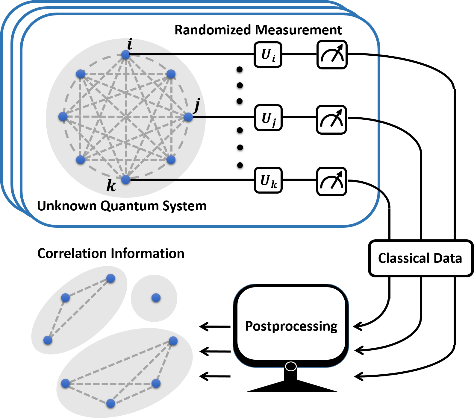
Figure 1: Illustration of the main idea. We present a protocol to measure the total correlation of an unknown multipartite quantum state in any partition. We perform qubitwise local randomized measurements on sequentially prepared states and thus obtain the classical measurement data. Using tailored data postprocessing strategies, the correlation information with respect to any chosen partition can be extracted.

One key amount of common interest is the total correlation within a multipartite quantum system Modi et al. 2010; Modi et al. 2012. Consider a joint quantum system consisting of kk subsystems {g1,g2,…,gk}\{g_{1},g_{2},\ldots,g_{k}\}, where each subsystem gig_{i} has local statistics specified by respective density operator ρi\rho_{i}. The joint system would be said to have no correlation if the joint state obeys ρ=⨂i=1kρi\rho=\bigotimes_{i=1}^{k}\rho_{i}, such that the global statistics is simply the product of its marginals. A state then possesses correlations if there exists deviation from this tensor product. A common measure of such deviation is the relative entropy, resulting in the quantifier S(ρ∥⨂i=1kρi)=∑iS(ρi)−S(ρ)S(\rho\|\bigotimes_{i=1}^{k}\rho_{i})=\sum_{i}S(\rho_{i})-S(\rho), where S⁡(⋅)S(\cdot) represents the von Neumann entropy. The quantity has found applications in quantum thermodynamics Goold et al. 2016 and many-body physics Chiara and Sanpera 2018; Goold et al. 2015, and the characterization of genuine multipartite correlation Bennett et al. 2011; Giorgi et al. 2011; Girolami et al. 2017. Nevertheless, the quantity remains difficult to access in practical experiments due to its inherent nonlinearity. Most approaches would require either interacting multiple copies of ρ\rho or state tomography, tasks that can be prohibitive if ρ\rho already presents the most challenging state one can synthesize on NISQ devices.

Here, we propose a quantifier of the total correlation — correlation overlap — whose technological accessibility is much closer to the synthesis of ρ\rho itself. In particular, our protocol only requires repeated synthesis of the same ρ\rho, together with local (qubitwise) random unitary evolution and computational measurements (see Fig. 1). Specifically, we show that the correlation overlap can be obtained by postprocessing the measurement data and the amount of data required is much less than the traditional quantum tomography. Meanwhile, the quantity itself maintains its operational meaning as a quantifier of total correlations, and can also be immediately adapted to measure how close candidate systems are to the maximally entangled.

II Definition

Recall that if a kk-partite quantum state ρ\rho is uncorrelated, it can be written as ⨂i=1kρi\bigotimes_{i=1}^{k}\rho_{i} with ρi=tri¯⁡(ρ)\rho_{i}=\tr_{\bar{i}}(\rho) being the reduced density matrix of the ii-th subsystem. Normally the relative entropy is adopted to quantify the distance between them Modi et al. 2010; Modi et al. 2012. The von Neumann entropy involved can be in principle acquired by the quantum state tomography, which is already challenging for systems with more than ten qubits. Thus, in order to make the measurement protocol scalable, one needs to avoid state tomography Mandal et al. 2020. Alternative entropy functions such as Re´\mathrm{\acute{e}}nyi entropy can be obtained by measuring the purity of the state Islam et al. 2015; Kaufman et al. 2016; Brydges et al. 2019. However, Re´\mathrm{\acute{e}}nyi entropy can violate the subadditivity Horodecki et al. 2009; Linden et al. 2013, which makes it nonideal for quantifying total correlation. Alternative approaches include uses of witnesses Guhne and Toth 2009; Friis et al. 2019 to detect the presence of certain correlations Huber and de Vicente 2013; Shahandeh et al. 2014; Lu et al. 2018; Zhou et al. 2019. These witnesses are typically tailored for specific classes of states (e.g. Tóth and Gühne 2005; Zhou et al. 2019) and are generally ineffective when applied to states without the preparation information Zhu et al. 2010; Dai et al. 2014; Zhou 2020.

Here we quantify the total correlation based on the fidelity between a given state ρ\rho and its marginals as follows:

C⁡(ρ)=−log⁡ℱ⁡(ρ,⨂i=1kρi),\displaystyle C(\rho)=-\log\mathcal{F}\left(\rho,\bigotimes_{i=1}^{k}\rho_{i}\right), (1)

with the fidelity Liang et al. 2019 being

ℱ⁡(ρ,⨂i=1kρi)=tr⁡(ρ​⨂i=1kρi)tr⁡(ρ2)⁡[∏i=1ktr⁡(ρi2)].\displaystyle\mathcal{F}\left(\rho,\bigotimes_{i=1}^{k}\rho_{i}\right)=\frac{\tr\left(\rho\bigotimes_{i=1}^{k}\rho_{i}\right)}{\sqrt{\tr(\rho^2)\left[\prod_{i=1}^{k}\tr(\rho_i^2)\right]}}. (2)

Notice that kk is not necessarily the number of qubits, but the number of subsystems under some partition. In Appendix B, we show that such total correlation measure satisfies certain key properties, such as faithfulness, no change under local unitary transformation, and additivity under tensor product. By taking the minimization on all possible bipartitions, one can also generalize it to quantify genuine multipartite correlation. We remark that other fidelity measures Liang et al. 2019 could also be adapted to define the total correlation where the measurability is the main concern.

The denominator of Eq. (2) is composed of a few purity terms, and there already exist effective methods to measure them Ekert et al. 2002; Brydges et al. 2019. The main contribution of this work is that we develop a protocol to effectively measure the numerator

Tk:=tr⁡(ρ​⨂i=1kρi)\displaystyle T_{k}:=\tr\left(\rho\bigotimes_{i=1}^{k}\rho_{i}\right) (3)

based on randomized measurements van Enk and Beenakker 2012; Elben et al. 2018; Brydges et al. 2019. We denote TkT_{k} as the correlation overlap (CRO), which is directly relative to the Hilbert-Schmidt distance

DHS​(ρ,⨂i=1kρi)=tr⁡(ρ2)+∏i=1ktr⁡(ρi2)−2​Tk.\displaystyle D_{\mathrm{HS}}\left(\rho,\bigotimes_{i=1}^{k}\rho_{i}\right)=\tr(\rho^2)+\prod_{i=1}^{k}\tr(\rho_i^2)-2T_{k}. (4)

When ρ\rho is a low-rank state Coles et al. 2019, such quantity can offer a tight bound of the trace distance between ρ\rho and its marginals, which can be further applied in the quantum independence testing Yu 2019. In addition, we also discuss the application of bipartite CRO in bipartite entanglement detection, and leave it in Appendix C.

III Efficient Estimation Protocols

We now show that the total correlation defined in the previous section can be effectively estimated, irrelevant of the party number kk. For simplicity of discussion, take the tripartite state ρA​B​C\rho_{ABC} as an example. Following the definition in Sec. II, the essential quantity one needs to evaluate is the tripartite CRO

T3=tr⁡[ρA​B​C​(ρA⊗ρB⊗ρC)].\displaystyle T_{3}=\tr\left[\rho_{ABC}(\rho_{A}\otimes\rho_{B}\otimes\rho_{C})\right]. (5)

The difficulty to measure T3T_{3} lies in that it is a nonlinear function of ρA​B​C\rho_{ABC} and thus cannot be obtained by measuring the observable on a single-copy state. In fact, given four identical states ρA​B​C⊗4\rho_{ABC}^{\otimes 4}, one can make a joint measurement among these copies Ekert et al. 2002,

T3\displaystyle T_{3} =tr⁡{SA⊗SB⊗SC​[ρA​B​C⊗(ρA⊗ρB⊗ρC)]}\displaystyle=\tr\left\{S_{A}\otimes S_{B}\otimes S_{C}\left[\rho_{ABC}\otimes(\rho_{A}\otimes\rho_{B}\otimes\rho_{C})\right]\right\} (6)
=tr⁡[SA(1,2)⊗SB(1,3)⊗SC(1,4)​(ρA​B​C⊗4)].\displaystyle=\tr\left[S_{A}^{(1,2)}\otimes S_{B}^{(1,3)}\otimes S_{C}^{(1,4)}(\rho_{ABC}^{\otimes 4})\right].

Here SA(1,2)S_{A}^{(1,2)} is the SWAP operator acting on the Hilbert space of the first two copies of subsystem AA, ℋA1⊗ℋA2\mathcal{H}_{A}^{1}\otimes\mathcal{H}_{A}^{2}, and acts trivially on the last two copies, SA(1,2)​|ψ⟩A1​|ϕ⟩A2=|ϕ⟩A1​|ψ⟩A2S_{A}^{(1,2)}|\psi\rangle_{A}^{1}|\phi\rangle_{A}^{2}=|\phi\rangle_{A}^{1}|\psi\rangle_{A}^{2}. And similarly for the other SWAP operators SB(1,3)S_{B}^{(1,3)} and SC(1,4)S_{C}^{(1,4)} (see Fig. 2(c) for an illustration).

This kind of measurement in general demands the preparation of identical copies of the state ρ\rho, and the joint measurements across the distinct copies, which is possible for the one-dimensional system and the few parties case, for example, k=2k=2 Islam et al. 2015; Kaufman et al. 2016. However, it is very challenging for the higher-dimensional system and for the number of parties kk being not small. In the following, we develop a measurement protocol based on randomized measurements van Enk and Beenakker 2012; Elben et al. 2018; Brydges et al. 2019; Huang et al. 2020, which only needs the preparation of singlecopies of the state ρ\rho. Randomized measurements find applications not only in quantum information, like entanglement negativity extraction Elben et al. 2020a; Zhou et al. 2020; Neven et al. 2021, entanglement detection Tran et al. 2016; Ketterer et al. 2019; Knips et al. 2020; Ketterer et al. 2020; Ketterer et al. 2021, Fisher information quantification Rath et al. 2021a; Yu et al. 2021, and quantum certification Elben et al. 2020b; Zhang et al. 2020; Zhang et al. 2021a, but also in quantum many-body physics Vermersch et al. 2019; Elben et al. 2020c; Cian et al. 2021; Garcia et al. 2021.

Global Measurement Protocol – We first propose a means to measure CRO using random unitary gates that act globally on each system. This protocol can then be subsequently modified to use only local unitary gates on each qubit with a modest sacrifice in error scaling. Our global measurement protocol works as follows: Sample and operate random unitary U=⨂i=1kUgiU=\bigotimes_{i=1}^{k}U_{g_{i}} on each subsystem gig_{i} for the total kk-partite system, independently, and then conduct computational basis measurement |s⟩=|sg1,sg2,…,sgk⟩\ket{s}=\ket{s_{g_1},s_{g_2},\dots,s_{g_k}} in a sequential manner. After sufficient repeating of the preparation and measurement, one can get the estimation of the conditional probability

Pr⁡(sg1,sg2,…,sgk|⨂i=1kUgi)=⟨s|​U​ρ​U†​|s⟩\displaystyle\mathrm{Pr}\left(s_{g_{1}},s_{g_{2}},\dots,s_{g_{k}}\Bigg|\bigotimes_{i=1}^{k}U_{g_{i}}\right)=\bra{s}U\rho U^{{\dagger}}\ket{s} (7)

and also its marginals Pr⁡(sgi|Ugi)\mathrm{Pr}(s_{g_{i}}|U_{g_{i}}) for the ii-th subsystem. The target quantity CRO TkT_{k}, can be written as the postprocessing of these conditional probabilities shown in Proposition 1, and we summarize the protocol in Algorithm 1.

Algorithm 1 Global Measurement Protocol for TkT_{k}
1: NU×NMN_{U}\times N_{M} sequentially prepared ρ\rho
2: Probability distribution of the measurement outcomes conditioned on the evolution unitary Pr⁡(sg1,sg2,…,sgk|⨂i=1kUgi)\mathrm{Pr}\left(s_{g_{1}},s_{g_{2}},\dots,s_{g_{k}}\Big|\bigotimes_{i=1}^{k}U_{g_{i}}\right) in Eq. (7).
3: for i=1​to​NUi=1~\text{{to}}~N_{U} do
4:   Randomly pick a unitary matrix U=⨂i=1kUgiU=\bigotimes_{i=1}^{k}U_{g_{i}}, with each Ugi∈ℋgiU_{g_{i}}\in\mathcal{H}_{g_{i}} sampled uniformly from the unitary 2-design ensemble.
5:   Operate UU on ρ\rho to get U​ρ​U†U\rho U^{\dagger}.
6:   for j=1​to​NMj=1~\text{{to}}~N_{M} do
7:    Measure U​ρ​U†U\rho U^{\dagger} in the computational basis {|s⟩=|sg1,sg2,…,sgk⟩}\{\ket{s}=\ket{s_{g_1},s_{g_2},\dots,s_{g_k}}\}.
8:    Record the measurement results.
9:   end for
10:   Estimate the probability and its marginals in Eq. (7).
11: end for
12: Do the data postprocessing given in Proposition 1 for TkT_{k}.
Proposition 1.

For a kk-partite state ρ\rho, the CRO TkT_{k} defined in Eq. (3), can be evaluated by postprocessing the measurement data, i.e., averaging the multiplication of the total and the marginal probabilities under the random unitary evolution as follows:

Tk=∑s,s′𝔼U[Pr⁡(s|U)​∏i=1kX𝑔i​(s𝑔i,s𝑔i′)​Pr​(s𝑔i′|Ugi)],\displaystyle T_{k}=\sum_{s,s^{\prime}}\mathop{\mathbb{E}}\limits_{U}\left[\mathrm{Pr}(s|U)\prod_{i=1}^{k}X_{\mathop{g}_{i}}(s_{\mathop{g}_{i}},s_{\mathop{g}_{i}}^{\prime})\ \mathrm{Pr}(s_{\mathop{g}_{i}}^{\prime}|U_{g_{i}})\right], (8)

with the function

X𝑔i​(s𝑔i,s𝑔i′)=−(−d𝑔i)δs𝑔i,s𝑔i′,\displaystyle X_{\mathop{g}_{i}}(s_{\mathop{g}_{i}},s_{\mathop{g}_{i}}^{\prime})=-(-d_{\mathop{g}_{i}})^{\delta_{s_{\mathop{g}_{i}},s_{\mathop{g}_{i}}^{\prime}}}, (9)

where d𝑔id_{\mathop{g}_{i}} is the dimension of the ii-th subsystem gig_{i}, and 𝔼U\mathbb{E}_{U} denotes averaging over unitary 2-design ensembles on each subsystem gig_{i} independently.

The detailed proof is left in Appendix D.2. The intuition is that by multiplying the probabilities in the postprocessing, one can virtually get a few copies of ρ\rho. Then by averaging on the random unitary, one can further generate permutation operators among virtual copies.

Refer to caption
Figure 2: Diagrammatic illustration of the proof of Proposition 1. Here, for simplicity, we take the tripartite state as an example. (a) is the diagram representation of Eq. (8). The small half circles with s,s′s,s^{\prime} inside represent the computational basis measurement. The dashed lines indicate that ρA​B​C\rho_{ABC} is not connected to ρA⊗ρB⊗ρC\rho_{A}\otimes\rho_{B}\otimes\rho_{C}. In (b), we use the cyclic property of the trace formula to put the random unitary evolution on XgX_{g}, for g∈{A,B,C}g\in\{A,B,C\}, defined in Eq. (9). The vertical gray dashed lines denote the periodic boundary condition, i.e., the trace. The colored dashed boxes are twofold twirling channels acting on XgX_{g}, which equal to the SWAP operators as shown in Eq. (10). As a result, we recover T3T_{3} in (c) with these SWAP operators represented by the “X”-shape cross in each dashed box, with the formula given in Eq. (6).

Here we sketch the proof outline using Fig. 2 for the T3T_{3} of the tripartite state ρA​B​C\rho_{ABC}. In Fig. 2(a), the conditional probabilities are multiplied, and the box labels the classical function Xg​(sg,sg′)X_{g}(s_{g},s_{g^{\prime}}) with g∈{A,B,C}g\in\{A,B,C\} for the subsystem. In Fig. 2(b), by using the cyclic property of the trace, we can effectively put the random unitary on the operator Xg=∑sg,sg′Xg​(sg,sg′)​|sg,sg′⟩​⟨sg,sg′|X_{g}=\sum_{s_{g},s_{g}^{\prime}}X_{g}(s_{g},s_{g}^{\prime})\ket{s_g,s_{g}'}\bra{s_g,s_{g}'}. In Fig. 2(c), we average on the unitary ensemble to generate a SWAP operator by the identity Elben et al. 2018; Elben et al. 2019,

Φ2(Xg):=𝔼Ug∈ℰ[Ug⊗2XgUg†⊗2]=Sg.\displaystyle\Phi^{2}(X_{g}):=\mathop{\mathbb{E}}\limits_{U_{g}\in\mathcal{E}}\left[U_{g}^{\otimes 2}X_{g}U_{g}^{\dagger\otimes 2}\right]=S_{g}. (10)

We denote this average on the two-copy Hilbert space as the “twrling” channel Φ2​(⋅)\Phi^{2}(\cdot). Note that the unitary ensemble ℰ\mathcal{E} need not be the Haar measure, and any unitary 2-design ensemble (such as the Clifford group DiVincenzo et al. 2002; Dankert et al. 2009) is sufficient, which is more practical compared with the previous work by some of us Zhou et al. 2020. If one naively generalizes the protocol there to measure the kk-partite CRO, a (k+1)(k+1)-design ensemble is needed. Unitary tt-design with t≥4t\geq 4 is still poorly understood Zhu et al. 2016, and the generation of these ensembles would need deep quantum circuit, which is quite impractical compared to the current protocol.

In real experiments, the sampling time NUN_{U} and the measurement time NMN_{M} as shown in Algorithm 1 are both finite; the postprocessing will be more delicate compared to Eq. (8) which corresponds to the case where NUN_{U} and NMN_{M} are infinite. We show how to construct an unbiased estimator for the scenario with finite NUN_{U} and NMN_{M} in Sec. IV. We remark that our protocol measures the fidelity of the state to its marginal, not with an unrelated state as in Ref. Elben et al. 2020b. By adequately utilizing the marginal distributions, our postprocessing shown in Sec. IV needs less state samples and thus is more efficient than directly applying the former one, say Ref. Elben et al. 2020b. Our protocol can be further generalized to local gate version, as discussed in the next section.

Local Measurement Protocol – We can further simplify the procedure above so that it makes use of only single-qubit random gates. Specifically, the global measurement protocol involves the need to sample random unitary on each subsystem, which may contain several qubits. This is challenging even for the moderate subsystem size. In contrast, the following local measurement protocol only involves random single-qubit Pauli measurement.

Recall that the essence of the global measurement protocol is to construct “virtual” SWAP operators across different copies in Eq. (6) by data postprocessing shown in Proposition 1. In fact, SWAP operator is factorizable. The big SWAP operator SS acting on nn-qubit pairs ℋ2⊗n⊗ℋ2⊗n\mathcal{H}_{2}^{\otimes n}\otimes\mathcal{H}_{2}^{\otimes n}, can be decomposed as S=⨂l=1nSlS=\bigotimes_{l=1}^{n}S_{l}, with SlS_{l} the small SWAP operator for the ii-th qubit pair (see Fig. 3 for an illustration). This fact enlightens us to substitute the random unitary, say UAU_{A} (also UBU_{B} and UCU_{C}) in Fig. 2, to the tensor product form UA=⨂l=1nAUlU_{A}=\bigotimes_{l=1}^{n_{A}}U_{l}, where each single-qubit unitary UlU_{l} is from the 2-design ensemble independently, similar for other subsystems BB and CC. Correspondingly, the postprocessing function X𝑔​(s𝑔,s𝑔′)X_{\mathop{g}}(s_{\mathop{g}},s_{\mathop{g}}^{\prime}) in Eq. (9) is modified to the multiplication of local functions as shown in Eq. (13).

For the general kk-partite state ρ\rho, suppose it contains n=∑i=1kngin=\sum_{i=1}^{k}n_{g_{i}} qubits with ii-th party having ngin_{g_{i}} qubits. We denote the computational basis as the nn-bit binary vector |s→⟩=|s1,s2,…,sn⟩,sl=0/1|\vec{s}\rangle=|s_{1},s_{2},\dots,s_{n}\rangle,s_{l}=0/1, and the state restricted on the ii-th party as |s→𝑔i⟩\ket{\vec{s}_{\mathop{g}_i}}. By modifying the global protocol in Algorithm 1, the local measurement protocol of CRO TkT_{k} is shown in Algorithm 2, and now we aim to obtain the following conditional probability

Pr⁡(s1,s2,…,sn|⨂l=1nUl)\displaystyle\mathrm{Pr}\left(s_{1},s_{2},\dots,s_{n}\Bigg|\bigotimes_{l=1}^{n}U_{l}\right) (11)

and its marginals Pr⁡(s→𝑔i|Ugi)\mathrm{Pr}(\vec{s}_{\mathop{g}_{i}}|U_{g_{i}}) with Ugi=⨂l∈giUlU_{g_{i}}=\bigotimes_{l\in g_{i}}U_{l}. The data postprocessing is summarized in Proposition 2.

Proposition 2.

Given a kk-partite state ρ\rho, the CRO TkT_{k} defined in Eq. (3), can be evaluated by postprocessing the measurement data, i.e., averaging the multiplication of the total and the marginal probabilities under the single-qubit random unitary evolution as follows.

Tk=∑s→,s→′𝔼U[Pr⁡(s→|U)​∏ikX~𝑔i​(s→𝑔i,s→𝑔i′)​Pr​(s→𝑔i′|Ugi)]\displaystyle T_{k}=\sum_{\vec{s},\vec{s}^{\prime}}\mathop{\mathbb{E}}\limits_{U}\left[\mathrm{Pr}(\vec{s}|U)\prod_{i}^{k}\tilde{X}_{\mathop{g}_{i}}(\vec{s}_{\mathop{g}_{i}},\vec{s}_{\mathop{g}_{i}}^{\prime})\mathrm{Pr}(\vec{s}_{\mathop{g}_{i}}^{\prime}|U_{g_{i}})\right] (12)

with the function

X~𝑔i​(s→𝑔i,s→𝑔i′):=∏l∈giXl​(sl,sl′)\displaystyle\tilde{X}_{\mathop{g}_{i}}(\vec{s}_{\mathop{g}_{i}},\vec{s}_{\mathop{g}_{i}}^{\prime}):=\prod_{l\in g_{i}}X_{l}(s_{l},s^{\prime}_{l}) (13)

where XlX_{l} is defined in Eq. (9) with dl=2d_{l}=2, and 𝔼U\mathbb{E}_{U} denotes averaging U=⨂l=1nUlU=\bigotimes_{l=1}^{n}U_{l} over unitary 2-design ensembles on each qubit independently.

Proposition 2 can be proved following the proof of Proposition 1, and the proof is left to Appendix D.3.

Algorithm 2 Local Measurement Protocol for TkT_{k}
1: NU×NMN_{U}\times N_{M} sequentially prepared ρ\rho
2: Probability distribution of the measurement outcomes conditioned on the evolution unitary Pr⁡(s1,s2,…,sn|⨂l=1nUl)\mathrm{Pr}\left(s_{1},s_{2},\dots,s_{n}\Bigg|\bigotimes_{l=1}^{n}U_{l}\right) in Eq. (11).
3: for i=1​to​NUi=1~\text{{to}}~N_{U} do
4:   Randomly pick a unitary matrix U=⨂l=1nUlU=\bigotimes_{l=1}^{n}U_{l}, with each Ul∈ℋlU_{l}\in\mathcal{H}_{l} on the ll-th qubit sampled uniformly from the unitary 2-design ensemble.
5:   Operate UU on ρ\rho to get U​ρ​U†U\rho U^{\dagger}.
6:   for j=1​to​NMj=1~\text{{to}}~N_{M} do
7:    Measure U​ρ​U†U\rho U^{\dagger} in the computational basis {|s⟩=|s1,s2,…,sn⟩\{\ket{s}=|s_{1},s_{2},\dots,s_{n}\rangle.
8:    Record the measurement results.
9:   end for
10:   Estimate the probability and its marginals in Eq. (11).
11: end for
12: Do the data postprocessing given in Proposition 2 for TkT_{k}.

Besides the practicality of the local measurement protocol, another advantage is that the measurement procedure and the postprocessing procedure are decoupled. In particular, one can choose to study the correlation for any partition of the system or the correlation information restricted on some subsystems in parallel, by only changing the postprocessing function.

Refer to caption
Figure 3: Here we provide a graphical example explaining how the global and local methods work. ρA​B​C\rho_{ABC} is an nine-qubit three-partite quantum state with each party containing three qubits. The curved lines with arrows in both ends denote SWAP operators. In global method (a), three-qubit SWAP operators are constructed using three-qubit random unitary matrix UAU_{A}, UBU_{B}, and UCU_{C}. While in local method (b), the three-qubit SWAP operators are decomposed into a tensor product of single-qubit SWAP operators, which can be constructed using single-qubit random unitary gates. Each colored dashed box represents a unitary 2-design.

IV Statistical analysis

In practical situations, the sampling times of the random unitary matrices NUN_{U}, and the number of the projective measurement NMN_{M} under a given unitary are both finite. The multiplication of them, NU​NMN_{U}N_{M}, quantifies how many copies of ρ\rho in total one needs to prepare in sequence. In this section, for clarity, we focus on the tripartite CRO in Eq. (5) and construct an unbiased estimator for it. We then analyze the variance of the estimator in this finite sampling scenario. The scaling of the variance respective to NUN_{U}, NMN_{M} and DD characterizes the sample complexity of our protocol. Similar analysis works for the cases of general kk-partite CRO. We use |s⟩=|sA,sB,sC⟩\ket{s}=\ket{s_A,s_B,s_C} to denote the computational basis of ℋ=ℋA⊗ℋB⊗ℋC\mathcal{H}=\mathcal{H}_{A}\otimes\mathcal{H}_{B}\otimes\mathcal{H}_{C}, where the total dimension is D=dA​dB​dCD=d_{A}d_{B}d_{C}. In the following, we first illustrate the estimation protocol with global unitary evolution, and then proceed to show how this can be converted to the one with the single-qubit measurements.

To construct an unbiased estimator, we first note that the postprocessing expression in Eq. (8) can be equivalently written as 44-time multiplication of the probability distribution,

T3=∑𝒔A,𝒔B,𝒔C\displaystyle T_{3}=\sum_{\bm{s}_{A},\bm{s}_{B},\bm{s}_{C}} XA(1,2)​(sA1,sA2)​XB(1,3)​(sB1,sB3)​XC(1,4)​(sC1,sC4)\displaystyle X^{(1,2)}_{A}(s^{1}_{A},s^{2}_{A})X^{(1,3)}_{B}(s^{1}_{B},s^{3}_{B})X^{(1,4)}_{C}(s_{C}^{1},s_{C}^{4}) (14)
×𝔼U[∏i=14Pr(sAi,sBi,sCi|UA,UB,UC)],\displaystyle\times\mathop{\mathbb{E}}\limits_{U}\left[\prod_{i=1}^{4}\mathrm{Pr}(s_{A}^{i},s_{B}^{i},s_{C}^{i}|U_{A},U_{B},U_{C})\right],

where we denote 𝒔A=(sA1,sA2,sA3,sA4)\bm{s}_{A}=(s_{A}^{1},s_{A}^{2},s_{A}^{3},s_{A}^{4}) as a 4-dit string with sAi∈{0,1,…,dA−1}s_{A}^{i}\in\{0,1,\dots,d_{A}-1\}, similar for 𝒔B\bm{s}_{B} and 𝒔C\bm{s}_{C}. XA(1,2)​(sA1,sA2)X^{(1,2)}_{A}(s_{A}^{1},s_{A}^{2}) is the function in Eq. (9) restricted on the first two indices, similar for XB(1,3)​(sB1,sB3)X_{B}^{(1,3)}(s_{B}^{1},s_{B}^{3}) and XC(1,4)​(sC1,sC4)X_{C}^{(1,4)}(s_{C}^{1},s_{C}^{4}).

In Algorithm 1, one samples NUN_{U} times of U=UA⊗UB⊗UCU=U_{A}\otimes U_{B}\otimes U_{C} to perform experiments. For the tt-th round of unitary sampling, one repeats the preparation and measurement for NMN_{M} times. For the ii-th time of measurement, we define a matrix-valued random variable

r^U​(i)=|s^U​(i)⟩​⟨s^U​(i)|,\hat{r}_{U}(i)=\ket{\hat{s}_U(i)}\bra{\hat{s}_U(i)}, (15)

where s^U​(i)\hat{s}_{U}(i) is a classical random variable with the conditional probability

Pr⁡(s|U)=⟨s|​U​ρA​B​C​U†​|s⟩,\mathrm{Pr}(s|U)=\bra{s}U\rho_{ABC}U^{{\dagger}}\ket{s}, (16)

to record the measurement result ss. For each random unitary choice, one finally gets NMN_{M} independent samples {r^U​(i)}i=1NM\{\hat{r}_{U}(i)\}_{i=1}^{N_{M}}. We then construct an estimator for T3T_{3} as follows

M^​(t)\displaystyle\hat{M}(t) =(NM4)−1​∑1≤i<j<k<l≤NMtr⁡{Q3​[r^U​(i)⊗r^U​(j)⊗r^U​(k)⊗r^U​(l)]}\displaystyle=\binom{N_{M}}{4}^{-1}\sum_{1\leq i<j<k<l\leq N_{M}}\tr\left\{Q_{3}\left[\hat{r}_{U}(i)\otimes\hat{r}_{U}(j)\otimes\hat{r}_{U}(k)\otimes\hat{r}_{U}(l)\right]\right\} (17)
=(NM4)−1​∑1≤i<j<k<l≤NMXA(1,2)​(s^U​(i),s^U​(j))​XB(1,3)​(s^U​(i),s^U​(k))​XC(1,4)​(s^U​(i),s^U​(l)),\displaystyle=\binom{N_{M}}{4}^{-1}\sum_{1\leq i<j<k<l\leq N_{M}}X^{(1,2)}_{A}\left(\hat{s}_{U}(i),\hat{s}_{U}(j)\right)X^{(1,3)}_{B}\left(\hat{s}_{U}(i),\hat{s}_{U}(k)\right)X^{(1,4)}_{C}\left(\hat{s}_{U}(i),\hat{s}_{U}(l)\right),

with

Q3:=(XA(1,2)⊗IA(3,4))⊗(XB(1,3)⊗IB(2,4))⊗(XC(1,4)⊗IC(2,3))Q_{3}:=\left(X_{A}^{(1,2)}\otimes I_{A}^{(3,4)}\right)\otimes\left(X_{B}^{(1,3)}\otimes I_{B}^{(2,4)}\right)\otimes\left(X_{C}^{(1,4)}\otimes I_{C}^{(2,3)}\right) (18)

being an observable on ℋ⊗4\mathcal{H}^{\otimes 4}. M^​(t)\hat{M}(t) is an unbiased estimator in the sense that 𝔼U,𝐬​[M^​(t)]=T3\mathbb{E}_{U,\mathbf{s}}\left[\hat{M}(t)\right]=T_{3}, with the expectation value taken for all random UU and measurement outputs. Since the estimators {M^​(t)}t=1NU\{\hat{M}(t)\}_{t=1}^{N_{U}} are independent and identically distributed, the final estimator is defined as M^=1NU​∑t=1NUM^​(t)\hat{M}=\frac{1}{N_{U}}\sum_{t=1}^{N_{U}}\hat{M}(t), which is naturally unbiased.

In the local measurement protocol, the unitaries on subsystems AA, BB and CC are substituted to products of the random unitaries on qubits. To construct the unbiased estimator for the local protocol, accordingly the postprocessing matrix QQ in Eq. (18) should be adjusted to

Q3,loc:=(X~A(1,2)⊗IA(3,4))⊗(X~B(1,3)⊗IB(2,4))⊗(X~C(1,4)⊗IC(2,3))Q_{3,\mathrm{loc}}:=\left(\tilde{X}_{A}^{(1,2)}\otimes I_{A}^{(3,4)}\right)\otimes\left(\tilde{X}_{B}^{(1,3)}\otimes I_{B}^{(2,4)}\right)\otimes\left(\tilde{X}_{C}^{(1,4)}\otimes I_{C}^{(2,3)}\right) (19)

with X~A(1,2)=⨂i=1nAXAi(1,2)\tilde{X}_{A}^{(1,2)}=\bigotimes_{i=1}^{n_{A}}X_{A_{i}}^{(1,2)} the product of the qubitwise XX operator. Similar as in Eq. (17), one can construct the final unbiased estimator M^L=1NU​∑t=1NUM^L​(t)\hat{M}_{L}=\frac{1}{N_{U}}\sum_{t=1}^{N_{U}}\hat{M}_{L}(t).

To construct the unbiased estimator for TkT_{k}, one just needs to extend the definition of Q3Q_{3} and Q3,locQ_{3,\mathrm{loc}} to the kk-partite scenario

Qk\displaystyle Q_{k} :=⨂i=2k+1(Xgi(1,i)⊗Igi(1,i)¯),\displaystyle:=\bigotimes_{i=2}^{k+1}\left(X_{g_{i}}^{(1,i)}\otimes I_{g_{i}}^{\overline{(1,i)}}\right), (20)
Qk,loc\displaystyle Q_{k,\mathrm{loc}} :=⨂i=2k+1(X~gi(1,i)⊗Igi(1,i)¯),\displaystyle:=\bigotimes_{i=2}^{k+1}\left(\tilde{X}_{g_{i}}^{(1,i)}\otimes I_{g_{i}}^{\overline{(1,i)}}\right),

where (1,i)¯\overline{(1,i)} is the complementary set of (1,i)(1,i) of {1,2,…,k+1}\{1,2,\dots,k+1\}. We further give the following result on the variance of these constructed estimators for TkT_{k}.

Proposition 3.

In the regime D≫NM≫kD\gg N_{M}\gg k, the variance of the unbiased estimators M^\hat{M} and M^L\hat{M}_{L} for the kk-partite CRO show the following scaling:

Var⁡(M^)=Θ⁡(DNU​NMk+1),\displaystyle\mathrm{Var}\left(\hat{M}\right)=\Theta(\frac{D}{N_{U}N_{M}^{k+1}}), (21)
Var⁡(M^L)=O⁡(Dlog2​3NU​NMk+1),\displaystyle\mathrm{Var}\left(\hat{M}_{L}\right)=O(\frac{D^{\log_{2}3}}{N_{U}N_{M}^{k+1}}),

where M^\hat{M} and M^L\hat{M}_{L} are constructed with the measurement data from the protocols in Algorithm 1 and Algorithm 2, respectively.

For the global random unitary case, we rigorously prove that the variance scales linearly with DD, NU−1N_{U}^{-1}, and NM−(k+1)N_{M}^{-(k+1)}; while for the local random unitary case, we provide an upper bound on the scaling. No matter in the global or the local case, such error scaling is much better than full tomography Haah et al. 2017. Inaddition, the variance decreases when increasing the party number kk, which is equivalent to the number of virtual copies of state. In Appendices E and F, we provide a detailed analysis of the statistical variance.

To support our theoretical analysis, we conduct numerical experiments for the local protocol, i.e., the random unitary matrix applied is the tensor product of the random qubit ones. The numerical results are shown in Fig. 4. In Fig. 4(a)-4(c), we choose the tripartite Greenberger-Horne-Zeilinger (GHZ) state, with an equal qubit number in each party, as the target state. The exact value T3=0.125T_{3}=0.125 is independent of the qubit number, so that the variance itself is suitable to quantify the quality of the estimation result. We first show how the variance changes with NUN_{U} when measuring a three-qubit GHZ state for different NMN_{M} in Fig. 4(a). These three lines with slopes about −1-1 are coincident with the conclusion in Proposition3 that Var⁡(M^L)∝NU−1\mathrm{Var}\left(\hat{M}_{L}\right)\propto N_{U}^{-1}. The variance decreases with the increase of NMN_{M}, the measurement times per unitary evolution. Then, by adjusting the qubit number of the GHZ state and with a fixed NM=10N_{M}=10, we also find that the variance increases for larger system dimension in Fig. 4(b).

To study how the variance scales with dimension DD when D≫NMD\gg N_{M}, we change the qubit number of the target GHZ state from 6 to 21 and set NU=100N_{U}=100 and NM=10N_{M}=10 in Fig. 4(c). The slope α=1.2587\alpha=1.2587 from the linear regression of log2⁡[Var⁡(M^L)]\log_{2}\left[\mathrm{Var}\left(\hat{M}_{L}\right)\right] and the qubit number nn. It indicates Var⁡(M^L)∝Dα\mathrm{Var}\left(\hat{M}_{L}\right)\propto D^{\alpha} with α≈1.26<log2​3\alpha\approx 1.26<\log_{2}3, which is consistent with our theoretical result in Proposition3. In Fig. 4(d), we take a six-qubit noisy WW state as an example, show the measurement results for different NMN_{M} with NU=100N_{U}=100, and find that our protocol can provide such high-quality measurement results as NM≥20N_{M}\geq 20.

Figure 4: Numerical results for the estimation of the tripartite CRO T3T_{3} in Eq. (5) with the local measurement protocol. (a) The variance scaling with NUN_{U} for different NMN_{M} when measuring the three-qubit GHZ state. (b) The variance scaling with NUN_{U} when measuring the GHZ state with different number of qubits, and NM=10N_{M}=10. (c) The variance dependence on the number of qubits of the measured GHZ state with NU=100N_{U}=100 and NM=10N_{M}=10. We linearly regress the data and obtain the slope α=1.2587\alpha=1.2587. (d) The estimation for the noisy state. We measure T3T_{3} of a six-qubit noisy WW state ρA​B​C=(1−p)​|W⟩​⟨W|+p26​I\rho_{ABC}=(1-p)|W\rangle\langle W|+\frac{p}{2^{6}}I with NU=100N_{U}=100 and different NMN_{M}.

V Application to Measuring Fidelity to Maximally Entangled States

Our protocol can also be modified to measure the fidelity between the candidate bipartite state, and that of a maximally entangled state,

|Ψ+⟩=1d​∑i=1d|i​i⟩,\displaystyle|\Psi^{+}\rangle=\frac{1}{\sqrt{d}}\sum_{i=1}^{d}|ii\rangle, (22)

on ℋA⊗ℋB\mathcal{H}_{A}\otimes\mathcal{H}_{B}. This fidelity is important in entanglement detection Guhne and Toth 2009 and many quantum communication tasks Horodecki et al. 2009. Prior methods need an ideally prepared state Elben et al. 2020b or fixed basis measurements. Utilizing random measurements, the maximally entangled state can be virtually produced by postprocessing, and randomness may make it more robust against the noise in the measurement basis.

Without loss of generality, we consider d=2nd=2^{n} with nn being the qubit number of each party. Recall that the outer product form of the SWAP operator is S=∑i,j=1d|i⟩​⟨j|⊗|j⟩​⟨i|S=\sum_{i,j=1}^{d}|i\rangle\langle j|\otimes|j\rangle\langle i|, and the maximally entangled state is proportional to the partial transpose of SS as follows.

|Ψ+⟩​⟨Ψ+|=\displaystyle|\Psi^{+}\rangle\langle\Psi^{+}|= 1d​∑i,j=1d|i⟩​⟨j|⊗|i⟩​⟨j|\displaystyle\frac{1}{d}\sum_{i,j=1}^{d}|i\rangle\langle j|\otimes|i\rangle\langle j| (23)
=\displaystyle= 1d​(∑i,j=1d|i⟩​⟨j|⊗|j⟩​⟨i|)TB=1d​STB,\displaystyle\frac{1}{d}\left(\sum_{i,j=1}^{d}|i\rangle\langle j|\otimes|j\rangle\langle i|\right)^{T_{B}}=\frac{1}{d}S^{T_{B}},

and the corresponding diagrams are shown in Figs. 5(a) and 5(b).

Suppose the state we actually produce is ρ∈ℋA⊗ℋB\rho\in\mathcal{H}_{A}\otimes\mathcal{H}_{B}. According to Eq. (23), the fidelity between ρ\rho and |Ψ+⟩|\Psi^{+}\rangle can be represented using SS as

tr⁡(ρ⁡|Ψ+⟩​⟨Ψ+|)=1d​tr⁡(ρ​STB).\displaystyle\tr\left(\rho|\Psi^{+}\rangle\langle\Psi^{+}|\right)=\frac{1}{d}\tr\left(\rho S^{T_{B}}\right). (24)

Recall that Eq. (10) shows that the SWAP operator can be effectively generated by randomized measurements. Hence the fidelity can be further rewritten as

tr⁡(ρ⁡|Ψ+⟩​⟨Ψ+|)=\displaystyle\tr\left(\rho|\Psi^{+}\rangle\langle\Psi^{+}|\right)= 1d​tr⁡(ρ​[Φ2​(X)]TB)\displaystyle\frac{1}{d}\tr\left(\rho[\Phi^{2}(X)]^{T_{B}}\right) (25)
=\displaystyle= 1d​tr⁡{ρ​𝔼U[(U⊗U)†​X​(U⊗U)]TB}\displaystyle\frac{1}{d}\tr\left\{\rho\mathop{\mathbb{E}}\limits_{U}\left[(U\otimes U)^{\dagger}X(U\otimes U)\right]^{T_{B}}\right\}
=\displaystyle= 1d​tr⁡{𝔼U[(U⊗U∗)​ρ​(U†⊗UT)]​X}.\displaystyle\frac{1}{d}\tr\left\{\mathop{\mathbb{E}}\limits_{U}\left[(U\otimes U^{*})\rho(U^{\dagger}\otimes U^{T})\right]X\right\}.

In the final equality, we use the fact that XX is a diagonal matrix such that XTB=XX^{T_{B}}=X, and also the cyclic property of trace to put the unitary evolution on the state (see Fig. 5 for an illustration).

Similar as for the local unitary protocol shown in Sec. III, one can apply the local random unitary U=⨂i=1nUiU=\bigotimes_{i=1}^{n}U_{i} here. As a result, the postprocessing matrix is substituted by X~​(s→A,s→B)=∏iXi​(siA,siB)=2n​(−2)−D⁡[s→A,s→B]\tilde{X}(\vec{s}_{A},\vec{s}_{B})=\prod_{i}X_{i}(s^{A}_{i},s^{B}_{i})=2^{n}(-2)^{-D[\vec{s}_{A},\vec{s}_{B}]} as in Eq. (13). Note that here the postprocessing function is on the measurement result of the two parties AA and BB, not on the different copies as before. We summarize the postprocessing under local random unitary as follows.

Refer to caption
Figure 5: Diagrammatic illustration of the derivation in Eq. (25). 𝔼U∈ℰ\mathbb{E}_{U\in\mathcal{E}} denotes averaging over (qubit) unitary 2-design and the dotted lines represent the transposition on the second subsystem. (a) d⁡|Ψ+⟩​⟨Ψ+|→d|\Psi^{+}\rangle\langle\Psi^{+}|\to (b) STB→S^{T_{B}}\to (c) [Φ2​(X)]TB=𝔼U[(U⊗U)​X​(U⊗U)†]TB→[\Phi^{2}(X)]^{T_{B}}=\mathop{\mathbb{E}}\limits_{U}\left[(U\otimes U)X(U\otimes U)^{\dagger}\right]^{T_{B}}\to (d) 𝔼U[(U⊗U∗)​XTB​(U†⊗UT)]→\mathop{\mathbb{E}}\limits_{U}\left[(U\otimes U^{*})X^{T_{B}}(U^{\dagger}\otimes U^{T})\right]\to (e) 𝔼U[(U⊗U∗)​X​(U†⊗UT)]\mathop{\mathbb{E}}\limits_{U}\left[(U\otimes U^{*})X(U^{\dagger}\otimes U^{T})\right].
Proposition 4.

For a bipartite state ρA​B\rho_{AB} with subsystems A and B both containing nn qubits, the fidelity of a state ρA​B\rho_{AB} with the maximally entangled state |Ψ+⟩\ket{\Psi^+} can be expressed by the following local randomized measurement result:

tr⁡(ρA​B​|Ψ+⟩​⟨Ψ+|)=∑s→A,s→B(−2)−D⁡[s→A,s→B]​𝔼UPr⁡(s→A,s→B|U),\displaystyle\tr\left(\rho_{AB}|\Psi^{+}\rangle\langle\Psi^{+}|\right)=\sum_{\vec{s}_{A},\vec{s}_{B}}(-2)^{-D[\vec{s}_{A},\vec{s}_{B}]}\mathop{\mathbb{E}}\limits_{U}\mathrm{Pr}(\vec{s}_{A},\vec{s}_{B}|U), (26)
Pr(s→A,s→B|U)=tr[(U⊗U∗)ρ(U†⊗UT)|s→A,s→B⟩⟨s→A,s→B|],\displaystyle\mathrm{Pr}(\vec{s}_{A},\vec{s}_{B}|U)=\tr\left[(U\otimes U^{*})\rho(U^{\dagger}\otimes U^{T})|\vec{s}_{A},\vec{s}_{B}\rangle\langle\vec{s}_{A},\vec{s}_{B}|\right],

where P⁡(s→A,s→B|U)P(\vec{s}_{A},\vec{s}_{B}|U) is the probability when measuring (U⊗U∗)​ρ​(U†⊗UT)(U\otimes U^{*})\rho(U^{\dagger}\otimes U^{T}) in the computational basis {|s→A,s→B⟩}\{|\vec{s}_{A},\vec{s}_{B}\rangle\}; the random unitary U=⨂i=1nUiU=\bigotimes_{i=1}^{n}U_{i} is a tensor product of unitaries on each qubit, where each UiU_{i} is sampled from a unitary 22-design.

Based on Proposition 4, we summarize the fidelity measurement protocol in Algorithm 3.

Algorithm 3 Fidelity with Local Measurement
1: NU×NMN_{U}\times N_{M} sequentially prepared ρA​B\rho_{AB} with subsystems AA and BB both containing nn qubits.
2: Probabilities measured in computational measurement basis under random unitary evolution Pr⁡(s→A,s→B|U)\mathrm{Pr}(\vec{s}_{A},\vec{s}_{B}|U).
3: for i=1​to​NUi=1~\text{{to}}~N_{U} do
4:   Randomly pick a unitary matrix U=⨂i=1nUiU=\bigotimes_{i=1}^{n}U_{i}, where UiU_{i} on each qubit forms a unitary 22-design. Operate U⊗U∗U\otimes U^{*} on ρ\rho to get (U⊗U∗)​ρ​(U†⊗UT)(U\otimes U^{*})\rho(U^{\dagger}\otimes U^{T}).
5:   for j=1​to​NMj=1~\text{{to}}~N_{M} do
6:    Measure (U⊗U∗)​ρ​(U†⊗UT)(U\otimes U^{*})\rho(U^{\dagger}\otimes U^{T}) in the computational basis {|s→A,s→B⟩}\{|\vec{s}_{A},\vec{s}_{B}\rangle\}.
7:    Record the measurement results.
8:   end for
9:   Estimate the probabilities Pr⁡(s→A,s→B|U)\mathrm{Pr}(\vec{s}_{A},\vec{s}_{B}|U).
10: end for
11: Do the data postprocessing according to Proposition 4.

In Appendix G, we also extend the randomized measurement method to estimate the concurrence Wootters 2001; Beacom and Vagins 2004 of an nn-qubit quantum state. This shows the broad application scenarios of the randomized measurements.

VI Discussion

In this work, we introduce an operationally meaningful quantifier of the total correlation within a multipartite quantum system motivated by experimental accessibility. Based on this definition, we design a protocol to estimate the total correlation of a candidate state using only classical postprocessing of data collected from randomized single-qubit measurements, and show that the number of measurements required is significantly lower than that of the state tomography. Taken together, the results provide an accessible tool for characterizing multipartite correlations in NISQ devices.

There are a number of interesting future directions. One direction involves observing that shadow estimation offers an alternative way to postprocess the measurement data under random unitary evolution Huang et al. 2020. Recently, there are enhancements of the error scaling of the shadow protocol by using prior knowledge of the observable Hadfield et al. 2020; Huang et al. 2021; Wu et al. 2021, or the intrinsic tensor-product structure of the underlying state for the nonlinear function estimation Garcia et al. 2021. It would be interesting to ascertain if these methodologies could provide further enhancement to estimating the total correlation measurement here, in situations where one has additional knowledge of the NISQ device Rath et al. 2021b.

The total correlation has many proposed applications. A recent framework for characterizing fine-grained structure or genuine multipartite correlation, for example, involves measuring how correlation changes depending on how one partitions the whole system Girolami et al. 2017; Bennett et al. 2011. Meanwhile, such correlation measure could be used as the cost function in the near-term variational algorithms to decouple the quantum system Yuan et al. 2019; Cerezo et al. 2020; Khatri et al. 2019; Zhang et al. 2021b. Both scenarios would require many costly repeated calls to estimate the correlation. Thus, a natural direction then is to investigate if our techniques provide the reduction to this cost. Meanwhile, many occasions invoke interest in specific types of correlations, such as those that are classical, or purely quantum mechanical, which is also interesting to further investigate with randomized measurements.

VII acknowledgments

We thank Arthur Jaffe and Xiongfeng Ma for the useful discussion. This research is supported by the Quantum Engineering Program QEP-SF3, National Research Foundation of Singapore under its NRF-ANR joint program (NRF2017-NRF-ANR004 VanQuTe), the Singapore Ministry of Education Tier 1 grant RG162/19, FQXi-RFP-IPW-1903 from the foundational Questions Institute and Fetzer Franklin Fund, a donor advised fund of Silicon Valley Community Foundation, the National Natural Science Foundation of China Grants No. 11875173 and No. 1217040781, and the National Key Research and Development Program of China Grants No. 2019QY0702 and No. 2017YFA0303903. Any opinions, findings and conclusions or recommendations expressed in this material are those of the author(s) and do not reflect the views of the National Research Foundation, Singapore.

References

  • Preskill (2018) J. Preskill, Quantum Computing in the NISQ era and beyond, Quantum 2, 79 (2018).
  • Horodecki et al. (2009) R. Horodecki, P. Horodecki, M. Horodecki, and K. Horodecki, Quantum entanglement, Rev. Mod. Phys. 81, 865 (2009).
  • Modi et al. (2012) K. Modi, A. Brodutch, H. Cable, T. Paterek, and V. Vedral, The classical-quantum boundary for correlations: Discord and related measures, Rev. Mod. Phys. 84, 1655 (2012).
  • Eisert et al. (2020) J. Eisert, D. Hangleiter, N. Walk, I. Roth, D. Markham, R. Parekh, U. Chabaud, and E. Kashefi, Quantum certification and benchmarking, Nature Reviews Physics 2, 382 (2020).
  • Kliesch and Roth (2021) M. Kliesch and I. Roth, Theory of quantum system certification, PRX Quantum 2, 010201 (2021).
  • Modi et al. (2010) K. Modi, T. Paterek, W. Son, V. Vedral, and M. Williamson, Unified view of quantum and classical correlations, Phys. Rev. Lett. 104, 080501 (2010).
  • Goold et al. (2016) J. Goold, M. Huber, A. Riera, L. del Rio, and P. Skrzypczyk, The role of quantum information in thermodynamics—a topical review, Journal of Physics A: Mathematical and Theoretical 49, 143001 (2016).
  • Chiara and Sanpera (2018) G. D. Chiara and A. Sanpera, Genuine quantum correlations in quantum many-body systems: a review of recent progress, Reports on Progress in Physics 81, 074002 (2018).
  • Goold et al. (2015) J. Goold, C. Gogolin, S. R. Clark, J. Eisert, A. Scardicchio, and A. Silva, Total correlations of the diagonal ensemble herald the many-body localization transition, Phys. Rev. B 92, 180202 (2015).
  • Bennett et al. (2011) C. H. Bennett, A. Grudka, M. Horodecki, P. Horodecki, and R. Horodecki, Postulates for measures of genuine multipartite correlations, Phys. Rev. A 83, 012312 (2011).
  • Giorgi et al. (2011) G. L. Giorgi, B. Bellomo, F. Galve, and R. Zambrini, Genuine quantum and classical correlations in multipartite systems, Phys. Rev. Lett. 107, 190501 (2011).
  • Girolami et al. (2017) D. Girolami, T. Tufarelli, and C. E. Susa, Quantifying genuine multipartite correlations and their pattern complexity, Phys. Rev. Lett. 119, 140505 (2017).
  • Mandal et al. (2020) S. Mandal, M. Narozniak, C. Radhakrishnan, Z.-Q. Jiao, X.-M. Jin, and T. Byrnes, Characterizing coherence with quantum observables, Phys. Rev. Research 2, 013157 (2020).
  • Islam et al. (2015) R. Islam, R. Ma, P. M. Preiss, M. Eric Tai, A. Lukin, M. Rispoli, and M. Greiner, Measuring entanglement entropy in a quantum many-body system, Nature 528, 77 (2015).
  • Kaufman et al. (2016) A. M. Kaufman, M. E. Tai, A. Lukin, M. Rispoli, R. Schittko, P. M. Preiss, and M. Greiner, Quantum thermalization through entanglement in an isolated many-body system, Science 353, 794 (2016).
  • Brydges et al. (2019) T. Brydges, A. Elben, P. Jurcevic, B. Vermersch, C. Maier, B. P. Lanyon, P. Zoller, R. Blatt, and C. F. Roos, Probing rényi entanglement entropy via randomized measurements, Science 364, 260 (2019).
  • Linden et al. (2013) N. Linden, M. Mosonyi, and A. Winter, The structure of rényi entropic inequalities, Proceedings of the Royal Society A: Mathematical, Physical and Engineering Sciences 469, 20120737 (2013).
  • Guhne and Toth (2009) O. Guhne and G. Toth, Entanglement detection, Physics Reports 474, 1 (2009).
  • Friis et al. (2019) N. Friis, G. Vitagliano, M. Malik, and M. Huber, Entanglement certification from theory to experiment, Nature Reviews Physics 1, 72 (2019).
  • Huber and de Vicente (2013) M. Huber and J. I. de Vicente, Structure of multidimensional entanglement in multipartite systems, Phys. Rev. Lett. 110, 030501 (2013).
  • Shahandeh et al. (2014) F. Shahandeh, J. Sperling, and W. Vogel, Structural quantification of entanglement, Phys. Rev. Lett. 113, 260502 (2014).
  • Lu et al. (2018) H. Lu, Q. Zhao, Z.-D. Li, X.-F. Yin, X. Yuan, J.-C. Hung, L.-K. Chen, L. Li, N.-L. Liu, C.-Z. Peng, Y.-C. Liang, X. Ma, Y.-A. Chen, and J.-W. Pan, Entanglement structure: Entanglement partitioning in multipartite systems and its experimental detection using optimizable witnesses, Phys. Rev. X 8, 021072 (2018).
  • Zhou et al. (2019) Y. Zhou, Q. Zhao, X. Yuan, and X. Ma, Detecting multipartite entanglement structure with minimal resources, npj Quantum Information 5, 1 (2019).
  • Tóth and Gühne (2005) G. Tóth and O. Gühne, Detecting genuine multipartite entanglement with two local measurements, Phys. Rev. Lett. 94, 060501 (2005).
  • Zhu et al. (2010) H. Zhu, Y. S. Teo, and B.-G. Englert, Minimal tomography with entanglement witnesses, Phys. Rev. A 81, 052339 (2010).
  • Dai et al. (2014) J. Dai, Y. L. Len, Y. S. Teo, B.-G. Englert, and L. A. Krivitsky, Experimental detection of entanglement with optimal-witness families, Phys. Rev. Lett. 113, 170402 (2014).
  • Zhou (2020) Y. Zhou, Entanglement detection under coherent noise: Greenberger-horne-zeilinger-like states, Phys. Rev. A 101, 012301 (2020).
  • Liang et al. (2019) Y.-C. Liang, Y.-H. Yeh, P. E. M. F. Mendonça, R. Y. Teh, M. D. Reid, and P. D. Drummond, Quantum fidelity measures for mixed states, Reports on Progress in Physics 82, 076001 (2019).
  • Ekert et al. (2002) A. K. Ekert, C. M. Alves, D. K. L. Oi, M. Horodecki, P. Horodecki, and L. C. Kwek, Direct estimations of linear and nonlinear functionals of a quantum state, Phys. Rev. Lett. 88, 217901 (2002).
  • van Enk and Beenakker (2012) S. J. van Enk and C. W. J. Beenakker, Measuring Tr​ρn\mathrm{Tr}{\rho}^{n} on single copies of ρ\rho using random measurements, Phys. Rev. Lett. 108, 110503 (2012).
  • Elben et al. (2018) A. Elben, B. Vermersch, M. Dalmonte, J. I. Cirac, and P. Zoller, Rényi entropies from random quenches in atomic hubbard and spin models, Phys. Rev. Lett. 120, 050406 (2018).
  • Coles et al. (2019) P. J. Coles, M. Cerezo, and L. Cincio, Strong bound between trace distance and hilbert-schmidt distance for low-rank states, Phys. Rev. A 100, 022103 (2019).
  • Yu (2019) N. Yu, Quantum closeness testing: A streaming algorithm and applications, arXiv:1904.03218 (2019).
  • Huang et al. (2020) H.-Y. Huang, R. Kueng, and J. Preskill, Predicting many properties of a quantum system from very few measurements, Nature Physics 16, 1050 (2020).
  • Elben et al. (2020a) A. Elben, R. Kueng, H.-Y. R. Huang, R. van Bijnen, C. Kokail, M. Dalmonte, P. Calabrese, B. Kraus, J. Preskill, P. Zoller, and B. Vermersch, Mixed-state entanglement from local randomized measurements, Phys. Rev. Lett. 125, 200501 (2020a).
  • Zhou et al. (2020) Y. Zhou, P. Zeng, and Z. Liu, Single-copies estimation of entanglement negativity, Phys. Rev. Lett. 125, 200502 (2020).
  • Neven et al. (2021) A. Neven, J. Carrasco, V. Vitale, C. Kokail, A. Elben, M. Dalmonte, P. Calabrese, P. Zoller, B. Vermersch, R. Kueng, and B. Kraus, Symmetry-resolved entanglement detection using partial transpose moments, npj Quantum Information 7, 152 (2021).
  • Tran et al. (2016) M. C. Tran, B. Dakić, W. Laskowski, and T. Paterek, Correlations between outcomes of random measurements, Phys. Rev. A 94, 042302 (2016).
  • Ketterer et al. (2019) A. Ketterer, N. Wyderka, and O. Gühne, Characterizing multipartite entanglement with moments of random correlations, Phys. Rev. Lett. 122, 120505 (2019).
  • Knips et al. (2020) L. Knips, J. Dziewior, W. Kobus, W. Laskowski, T. Paterek, P. J. Shadbolt, H. Weinfurter, and J. D. A. Meinecke, Multipartite entanglement analysis from random correlations, npj Quantum Information 6, 51 (2020).
  • Ketterer et al. (2020) A. Ketterer, N. Wyderka, and O. Gühne, Entanglement characterization using quantum designs, Quantum 4, 325 (2020).
  • Ketterer et al. (2021) A. Ketterer, S. Imai, N. Wyderka, and O. Gühne, Statistically significant tests of multiparticle quantum correlations based on randomized measurements, arXiv:2012.12176 [quant-ph] (2021).
  • Rath et al. (2021a) A. Rath, C. Branciard, A. Minguzzi, and B. Vermersch, Quantum fisher information from randomized measurements, Phys. Rev. Lett. 127, 260501 (2021a).
  • Yu et al. (2021) M. Yu, D. Li, J. Wang, Y. Chu, P. Yang, M. Gong, N. Goldman, and J. Cai, Experimental estimation of the quantum fisher information from randomized measurements, arXiv:2104.00519 (2021).
  • Elben et al. (2020b) A. Elben, B. Vermersch, R. van Bijnen, C. Kokail, T. Brydges, C. Maier, M. K. Joshi, R. Blatt, C. F. Roos, and P. Zoller, Cross-platform verification of intermediate scale quantum devices, Phys. Rev. Lett. 124, 010504 (2020b).
  • Zhang et al. (2020) W.-H. Zhang, C. Zhang, Z. Chen, X.-X. Peng, X.-Y. Xu, P. Yin, S. Yu, X.-J. Ye, Y.-J. Han, J.-S. Xu, G. Chen, C.-F. Li, and G.-C. Guo, Experimental optimal verification of entangled states using local measurements, Phys. Rev. Lett. 125, 030506 (2020).
  • Zhang et al. (2021a) T. Zhang, J. Sun, X.-X. Fang, X.-M. Zhang, X. Yuan, and H. Lu, Experimental quantum state measurement with classical shadows, Phys. Rev. Lett. 127, 200501 (2021a).
  • Vermersch et al. (2019) B. Vermersch, A. Elben, L. M. Sieberer, N. Y. Yao, and P. Zoller, Probing scrambling using statistical correlations between randomized measurements, Phys. Rev. X 9, 021061 (2019).
  • Elben et al. (2020c) A. Elben, J. Yu, G. Zhu, M. Hafezi, F. Pollmann, P. Zoller, and B. Vermersch, Many-body topological invariants from randomized measurements in synthetic quantum matter, Science Advances 6, eaaz3666 (2020c).
  • Cian et al. (2021) Z.-P. Cian, H. Dehghani, A. Elben, B. Vermersch, G. Zhu, M. Barkeshli, P. Zoller, and M. Hafezi, Many-body chern number from statistical correlations of randomized measurements, Phys. Rev. Lett. 126, 050501 (2021).
  • Garcia et al. (2021) R. J. Garcia, Y. Zhou, and A. Jaffe, Quantum scrambling with classical shadows, Phys. Rev. Research 3, 033155 (2021).
  • Elben et al. (2019) A. Elben, B. Vermersch, C. F. Roos, and P. Zoller, Statistical correlations between locally randomized measurements: A toolbox for probing entanglement in many-body quantum states, Phys. Rev. A 99, 052323 (2019).
  • DiVincenzo et al. (2002) D. P. DiVincenzo, D. W. Leung, and B. M. Terhal, Quantum data hiding, IEEE Transactions on Information Theory 48, 580 (2002).
  • Dankert et al. (2009) C. Dankert, R. Cleve, J. Emerson, and E. Livine, Exact and approximate unitary 2-designs and their application to fidelity estimation, Phys. Rev. A 80, 012304 (2009).
  • Zhu et al. (2016) H. Zhu, R. Kueng, M. Grassl, and D. Gross, The clifford group fails gracefully to be a unitary 4-design, arXiv:1609.08172 (2016).
  • Haah et al. (2017) J. Haah, A. W. Harrow, Z. Ji, X. Wu, and N. Yu, Sample-optimal tomography of quantum states, IEEE Transactions on Information Theory 63, 5628 (2017).
  • Wootters (2001) W. K. Wootters, Entanglement of formation and concurrence, Quantum Inf. Comput. 1, 27 (2001).
  • Beacom and Vagins (2004) J. F. Beacom and M. R. Vagins, Antineutrino spectroscopy with large water Čerenkov detectors, Phys. Rev. Lett. 93, 171101 (2004).
  • Hadfield et al. (2020) C. Hadfield, S. Bravyi, R. Raymond, and A. Mezzacapo, Measurements of quantum hamiltonians with locally-biased classical shadows, arXiv:2006.15788 (2020).
  • Huang et al. (2021) H.-Y. Huang, R. Kueng, and J. Preskill, Efficient estimation of pauli observables by derandomization, arXiv:2103.07510 (2021).
  • Wu et al. (2021) B. Wu, J. Sun, Q. Huang, and X. Yuan, Overlapped grouping measurement: A unified framework for measuring quantum states, arXiv:2105.13091 (2021).
  • Rath et al. (2021b) A. Rath, R. van Bijnen, A. Elben, P. Zoller, and B. Vermersch, Importance sampling of randomized measurements for probing entanglement, Phys. Rev. Lett. 127, 200503 (2021b).
  • Yuan et al. (2019) X. Yuan, S. Endo, Q. Zhao, Y. Li, and S. C. Benjamin, Theory of variational quantum simulation, Quantum 3, 191 (2019).
  • Cerezo et al. (2020) M. Cerezo, A. Arrasmith, R. Babbush, S. C. Benjamin, S. Endo, K. Fujii, J. R. McClean, K. Mitarai, X. Yuan, L. Cincio, et al., Variational quantum algorithms, arXiv:2012.09265 (2020).
  • Khatri et al. (2019) S. Khatri, R. LaRose, A. Poremba, L. Cincio, A. T. Sornborger, and P. J. Coles, Quantum-assisted quantum compiling, Quantum 3, 140 (2019).
  • Zhang et al. (2021b) Z.-J. Zhang, T. H. Kyaw, J. Kottmann, M. Degroote, and A. Aspuru-Guzik, Mutual information-assisted adaptive variational quantum eigensolver, Quantum Science and Technology (2021b).
  • Zyczkowski and Kus (1994) K. Zyczkowski and M. Kus, Random unitary matrices, Journal of Physics A: Mathematical and General 27, 4235 (1994).
  • Goodman and Wallach (2000) R. Goodman and N. R. Wallach, Representations and invariants of the classical groups (Cambridge University Press, 2000).
  • Gu (2013) Y. Gu, Moments of random matrices and weingarten functions, Ph.D. thesis (2013).
  • Lindner and Rodger (2017) C. C. Lindner and C. A. Rodger, Design theory (CRC press, 2017).
  • Wood et al. (2015) C. J. Wood, J. D. Biamonte, and D. G. Cory, Tensor networks and graphical calculus for open quantum systems, Quantum Information & Computation 15, 759 (2015).
  • Shapourian et al. (2021) H. Shapourian, S. Liu, J. Kudler-Flam, and A. Vishwanath, Entanglement negativity spectrum of random mixed states: A diagrammatic approach, PRX Quantum 2, 030347 (2021).
  • Zhang et al. (2008) C.-J. Zhang, Y.-S. Zhang, S. Zhang, and G.-C. Guo, Entanglement detection beyond the computable cross-norm or realignment criterion, Phys. Rev. A 77, 060301 (2008).
  • Kai and Wu (2002) C. Kai and L. A. Wu, A matrix realignment method for recognizing entanglement, Quantum Information and Computation 3, 193 (2002).
  • de Vicente (2008) J. I. de Vicente, Further results on entanglement detection and quantification from the correlation matrix criterion, Journal of Physics A: Mathematical and Theoretical 41, 065309 (2008).
  • Aolita and Mintert (2006) L. Aolita and F. Mintert, Measuring multipartite concurrence with a single factorizable observable, Phys. Rev. Lett. 97, 050501 (2006).

Appendix A Preliminaries

A.1 Integral of random unitary matrix

A random unitary matrix is a random variable in the space of a unitary matrix Zyczkowski and Kus 1994; Haar measure means that the probability distribution is uniform. Based on the definition of Haar-measured random unitary matrix, here we introduce a tt-fold twirling channel,

Φt(O)=∫HaardUU⊗tOU†⊗t,\displaystyle\Phi^{t}(O)=\int_{\mathrm{Haar}}dUU^{\otimes t}OU^{\dagger\otimes t}, (27)

where U∈ℋdU\in\mathcal{H}_{d} and OO is a linear operator acting on ℋd⊗t\mathcal{H}_{d}^{\otimes t}. According to Schur-Weyl duality Goodman and Wallach 2000; Kliesch and Roth 2021, such twirling channel is equivalent to the operation that projects OO into the symmetric subspace. So we have

Φt(O)=∫HaardUU⊗tOU†⊗t=∑π,σ∈𝒮tCπ,σtr⁡(Wπ​O)Wσ.\displaystyle\Phi^{t}(O)=\int_{\mathrm{Haar}}dUU^{\otimes t}OU^{\dagger\otimes t}=\sum_{\pi,\sigma\in\mathcal{S}_{t}}C_{\pi,\sigma}\tr(W_\pi O)W_{\sigma}. (28)

Where 𝒮t\mathcal{S}_{t} is the tt-th order permutation group, Cπ,σC_{\pi,\sigma} is the element of the Weingarten matrix Gu 2013, and WπW_{\pi} is the permutation operator corresponding to π\pi. By adjusting OO, one can generate any permutation operators; this is the core idea of the estimation protocol proposed in Sec. III.

Generally speaking, it is impractical to randomly pick an element in unitary space. Fortunately, it has been proved that a tt-fold twirling channel can be realized by averaging over a unitary ensemble ℰ\mathcal{E} within which the elements are all fixed unitary matrices, which we call ℰ\mathcal{E} unitary tt-design Lindner and Rodger 2017.

Φtℰ(O)=1|ℰ|∑U∈ℰU⊗tOU†⊗t=𝔼U∈ℰ(U⊗tOU†⊗t)=Φt(O),\displaystyle\Phi^{t}_{\mathcal{E}}(O)=\frac{1}{|\mathcal{E}|}\sum_{U\in\mathcal{E}}U^{\otimes t}OU^{\dagger\otimes t}=\mathop{\mathbb{E}}\limits_{U\in\mathcal{E}}\left(U^{\otimes t}OU^{\dagger\otimes t}\right)=\Phi^{t}(O), (29)

where |ℰ||\mathcal{E}| denotes the size of ℰ\mathcal{E}. This fact further reduces the difficulty of implementing twirling channel in real experiments. It is worth mentioning that the Clifford group is a unitary 33-design and a unitary tt-design is also an unitary mm-design with m<tm<t.

A.2 Tensor network basics

Tensor network is one of the graphical methods helping us to deal with tensor calculation Wood et al. 2015; Shapourian et al. 2021. In tensor networks, a tensor is represented as a box with open legs, which are indices of this tensor. For example, ρA​B​C=∑i,j,k,i′,j′,k′ρi​j​k,i′​j′​k′​|i​j​k⟩​⟨i′​j′​k′|\rho_{ABC}=\sum_{i,j,k,i^{\prime},j^{\prime},k^{\prime}}\rho_{ijk,i^{\prime}j^{\prime}k^{\prime}}|ijk\rangle\langle i^{\prime}j^{\prime}k^{\prime}| is represented as a box with six legs, three of which are left, representing row indices i,j,ki,j,k, and the other three are right, representing column indices i′,j′,k′i^{\prime},j^{\prime},k^{\prime}. Open legs represent the noncontracting indices, so the connection of legs is the contraction of indices. For example, tensor A​BAB is graphically represented by connecting the right legs of box AA and the left legs of box BB. tr⁡(A)=∑iAi,i\tr(A)=\sum_{i}A_{i,i} is the contraction of the row and column index of AA, which can be represented by connecting the left and right legs of box AA. In addition, tensor product is the operation that does not contract indices. So, to represent A⊗BA\otimes B, we just put boxes AA and BB together.

Refer to caption
Figure 6: (a) ρA​B​C=∑i,j,k,i′,j′,k′ρi​j​k,i′​j′​k′​|i​j​k⟩​⟨i′​j′​k′|\rho_{ABC}=\sum_{i,j,k,i^{\prime},j^{\prime},k^{\prime}}\rho_{ijk,i^{\prime}j^{\prime}k^{\prime}}|ijk\rangle\langle i^{\prime}j^{\prime}k^{\prime}|. (b) A​BAB. (c) tr⁡(A)\tr(A). (d) A⊗BA\otimes B

.

The unnormalized maximally entangled state (UMES) and SWAP operator are two commonly used operators. UMES d​|Ψ+⟩=∑i=1|i​i⟩\sqrt{d}|\Psi^{+}\rangle=\sum_{i=1}|ii\rangle is represented as a semicircle with both ends to the left, where dd is the dimension of Hilbert space. Many operations can be represented using UMES. Take A=∑i,jAi,j​|i⟩​⟨j|A=\sum_{i,j}A_{i,j}|i\rangle\langle j| as an example:

d⁡⟨Ψ+|A|Ψ+⟩=∑k⟨k​k|∑i,jAi,j|i⟩​⟨j|​∑l|l​l⟩=∑i,jAi,j​∑k,l⟨k⁡|i⟩​⟨j⁡|l⟩|​k⟩​⟨l|=∑i,jAi,j​|j⟩​⟨i|=AT\displaystyle d\langle\Psi^{+}|A|\Psi^{+}\rangle=\sum_{k}\langle kk|\sum_{i,j}A_{i,j}|i\rangle\langle j|\sum_{l}|ll\rangle=\sum_{i,j}A_{i,j}\sum_{k,l}\langle k|i\rangle\langle j|l\rangle|k\rangle\langle l|=\sum_{i,j}A_{i,j}|j\rangle\langle i|=A^{T} (30)

and

d⟨Ψ+|A⊗I|Ψ+⟩=∑k⟨kk|∑i,jAi,j|i⟩⟨j|⊗I∑l|ll⟩=∑i,jAi,j∑k,l⟨k|i⟩⟨j|l⟩⟨k|l⟩=∑iAi,i=tr⁡(A).\displaystyle d\langle\Psi^{+}|A\otimes I|\Psi^{+}\rangle=\sum_{k}\langle kk|\sum_{i,j}A_{i,j}|i\rangle\langle j|\otimes I\sum_{l}|ll\rangle=\sum_{i,j}A_{i,j}\sum_{k,l}\langle k|i\rangle\langle j|l\rangle\langle k|l\rangle=\sum_{i}A_{i,i}=\tr(A). (31)

tr⁡(A)\tr(A) has been shown in Fig. 6(c). SWAP SS, exchanging two indices, can be graphically represented with two crossed curved lines. Using this representation, one can easily prove that tr⁡[S⁡(A⊗B)]=tr⁡(A​B)\tr[S(A\otimes B)]=\tr(AB), as shown in Fig. 7.

Refer to caption
Figure 7: (a) d​|Ψ+⟩=∑i=1|i​i⟩\sqrt{d}|\Psi^{+}\rangle=\sum_{i=1}|ii\rangle. (b) ATA^{T}. (c) SS. (d) tr⁡[S⁡(A⊗B)]=tr⁡(A​B)\tr[S(A\otimes B)]=\tr(AB).

Appendix B The property of total correlation measure defined in Eq. (1)

Recall that we take C⁡(ρ)=−log2⁡ℱ⁡(ρ,⨂i=1kρi)C(\rho)=-\log_{2}\mathcal{F}\left(\rho,\bigotimes_{i=1}^{k}\rho_{i}\right), and the fidelity measure could be

ℱmax​(ρ,σ)=tr⁡(ρ​σ)max⁡{tr⁡(ρ2),tr⁡(σ2)}\displaystyle\mathcal{F}_{\max}\left(\rho,\sigma\right)=\frac{\tr\left(\rho\sigma\right)}{\max\{\tr(\rho^2),\tr(\sigma^2)\}} (32)

and

ℱGM​(ρ,σ)=tr⁡(ρ​σ)tr⁡(ρ2)​tr⁡(σ2),\displaystyle\mathcal{F}_{\mathrm{GM}}\left(\rho,\sigma\right)=\frac{\tr\left(\rho\sigma\right)}{\sqrt{\tr(\rho^2)\tr(\sigma^2)}}, (33)

which is the one used in the main text. Note that the difference is that the denominator is either maximization or geometric mean of the purity, and one can also choose other fidelity measures Liang et al. 2019. We take C⁡(ρ)=−log2​ℱGM​(ρ,⨂i=1kρi)C(\rho)=-\log_{2}\mathcal{F}_{\text{GM}}\left(\rho,\bigotimes_{i=1}^{k}\rho_{i}\right) as an example to discuss its property. The discussion of C⁡(ρ)=−log2​ℱmax​(ρ,⨂i=1kρi)C(\rho)=-\log_{2}\mathcal{F}_{\text{max}}\left(\rho,\bigotimes_{i=1}^{k}\rho_{i}\right) is quite similar.

  1. (1)

    C⁡(ρ)C(\rho) is a faithful total correlation measure, C⁡(ρ)=0C(\rho)=0 iff ρ=⨂i=1kρi\rho=\bigotimes_{i=1}^{k}\rho_{i}, and non-negative for any ρ\rho. This property directly follows from the property of fidelity: ℱGM​(ρ,σ)<1\mathcal{F}_{\text{GM}}(\rho,\sigma)<1, ∀ρ,σ\forall\rho,\sigma and ℱGM​(ρ,σ)=1\mathcal{F}_{\text{GM}}(\rho,\sigma)=1 iff ρ=σ\rho=\sigma.

  2. (2)

    Adding a new party ρk+1\rho_{k+1} to a kk-partite state ρ\rho will not cause the increase of the total correlation in the resulting (k+1)(k+1)-partite tensor state ρ⊗ρk+1\rho\otimes\rho_{k+1}, i.e. C⁡(ρ⊗ρk+1)=C⁡(ρ)C(\rho\otimes\rho_{k+1})=C(\rho).

    Proof.
    ℱGM​(ρ⊗ρk+1,⨂i=1kρi⊗ρk+1)\displaystyle\mathcal{F}_{\text{GM}}(\rho\otimes\rho_{k+1},\bigotimes_{i=1}^{k}\rho_{i}\otimes\rho_{k+1}) =tr⁡[(ρ⊗ρk+1)​(⨂i=1kρi⊗ρk+1)]tr⁡[(ρ⊗ρk+1)2]​tr⁡[(⨂i=1kρi⊗ρk+1)2]\displaystyle=\frac{\tr\left[(\rho\otimes\rho_{k+1})(\bigotimes_{i=1}^{k}\rho_{i}\otimes\rho_{k+1})\right]}{\sqrt{\tr\left[(\rho\otimes\rho_{k+1})^{2}\right]\tr\left[(\bigotimes_{i=1}^{k}\rho_{i}\otimes\rho_{k+1})^{2}\right]}} (34)
    =tr⁡(ρ​⨂i=1kρi)tr⁡ρ2​∏i=1ktr⁡ρi2​tr⁡ρk+12tr⁡ρk+12\displaystyle=\frac{\tr\left(\rho\bigotimes_{i=1}^{k}\rho_{i}\right)}{\sqrt{\tr\rho^{2}\prod_{i=1}^{k}\tr\rho_{i}^{2}}}\frac{\tr\rho_{k+1}^{2}}{\tr\rho_{k+1}^{2}}
    =ℱGM​(ρ,⨂i=1kρi).\displaystyle=\mathcal{F}_{\text{GM}}(\rho,\bigotimes_{i=1}^{k}\rho_{i}).

    Hence

    C⁡(ρ⊗ρk+1)=−log2​ℱGM​(ρ⊗ρk+1,⨂i=1kρi⊗ρk+1)=−log2​ℱGM​(ρ,⨂i=1kρi)=C⁡(ρ).\displaystyle C(\rho\otimes\rho_{k+1})=-\log_{2}\mathcal{F}_{\text{GM}}(\rho\otimes\rho_{k+1},\bigotimes_{i=1}^{k}\rho_{i}\otimes\rho_{k+1})=-\log_{2}\mathcal{F}_{\text{GM}}(\rho,\bigotimes_{i=1}^{k}\rho_{i})=C(\rho). (35)

    ∎

  3. (3)

    C⁡(ρ)C(\rho) is not changed under local unitary transformation, i.e. C⁡(⨂i=1kui​ρ​⨂i=1kui†)=C⁡(ρ)C(\bigotimes_{i=1}^{k}u_{i}\rho\bigotimes_{i=1}^{k}u_{i}^{\dagger})=C(\rho).

  4. (4)

    Local quantum channel, i.e., ⨂i=1kΛi\bigotimes_{i=1}^{k}\Lambda_{i}, cannot create total correlation in uncorrelated kk-partite state ρ=⨂i=1kρi\rho=\bigotimes_{i=1}^{k}\rho_{i}.

    Proof.

    Acting the local channel on the uncorrelated state, the resulting state is still uncorrelated:

    ⨂i=1kΛi​(⨂i=1kρi)=⨂i=1kΛi​(ρi).\displaystyle\bigotimes_{i=1}^{k}\Lambda_{i}\left(\bigotimes_{i=1}^{k}\rho_{i}\right)=\bigotimes_{i=1}^{k}\Lambda_{i}\left(\rho_{i}\right). (36)

    Therefore, the faithfulness of ℱGM​(⋅)\mathcal{F}_{\text{GM}}(\cdot) directly leads to the invariance of total correlation:

    C⁡[⨂i=1kΛi​(⨂i=1kρi)]=C⁡(⨂i=1kΛi​(ρi))=C⁡(⨂i=1kρi)=0.\displaystyle C\left[\bigotimes_{i=1}^{k}\Lambda_{i}\left(\bigotimes_{i=1}^{k}\rho_{i}\right)\right]=C\left(\bigotimes_{i=1}^{k}\Lambda_{i}\left(\rho_{i}\right)\right)=C\left(\bigotimes_{i=1}^{k}\rho_{i}\right)=0. (37)

    ∎

  5. (5)

    C⁡(ρ)C(\rho) is additive under the tensor product. The (k+l)(k+l)-partite total correlation C⁡(ρ⊗σ)C(\rho\otimes\sigma) equals the sum over of the kk-partite total correlation C⁡(ρ)C(\rho) and l-partite total correlation C⁡(σ)C(\sigma).

    Proof.
    ℱGM​(ρ⊗σ,⨂i=1kρi⊗⨂i=1lσi)\displaystyle\mathcal{F}_{\text{GM}}(\rho\otimes\sigma,\bigotimes_{i=1}^{k}\rho_{i}\otimes\bigotimes_{i=1}^{l}\sigma_{i}) =tr⁡[(ρ⊗σ)​(⨂i=1kρi⊗⨂i=1lσi)]tr⁡[(ρ⊗σ)2]​tr⁡[(⨂i=1kρi⊗⨂i=1lσi)2]\displaystyle=\frac{\tr\left[(\rho\otimes\sigma)(\bigotimes_{i=1}^{k}\rho_{i}\otimes\bigotimes_{i=1}^{l}\sigma_{i})\right]}{\sqrt{\tr\left[(\rho\otimes\sigma)^{2}\right]\tr\left[(\bigotimes_{i=1}^{k}\rho_{i}\otimes\bigotimes_{i=1}^{l}\sigma_{i})^{2}\right]}} (38)
    =tr⁡(ρ​⨂i=1kρi)tr⁡ρ2​∏i=1ktr⁡ρi2​tr⁡(σ​⨂i=1lσi)tr⁡σ2​∏i=1ltr⁡σi2\displaystyle=\frac{\tr\left(\rho\bigotimes_{i=1}^{k}\rho_{i}\right)}{\sqrt{\tr\rho^{2}\prod_{i=1}^{k}\tr\rho_{i}^{2}}}\frac{\tr\left(\sigma\bigotimes_{i=1}^{l}\sigma_{i}\right)}{\sqrt{\tr\sigma^{2}\prod_{i=1}^{l}\tr\sigma_{i}^{2}}}
    =ℱGM​(ρ,⨂i=1kρi)​ℱGM​(σ,⨂i=1lσi).\displaystyle=\mathcal{F}_{\text{GM}}(\rho,\bigotimes_{i=1}^{k}\rho_{i})\mathcal{F}_{\text{GM}}(\sigma,\bigotimes_{i=1}^{l}\sigma_{i}).

    Hence,

    C⁡(ρ⊗σ)\displaystyle C(\rho\otimes\sigma) =−log2​ℱGM​(ρ⊗σ,⨂i=1kρi⊗⨂i=1lσi)\displaystyle=-\log_{2}\mathcal{F}_{\text{GM}}(\rho\otimes\sigma,\bigotimes_{i=1}^{k}\rho_{i}\otimes\bigotimes_{i=1}^{l}\sigma_{i}) (39)
    =−log2​ℱGM​(ρ,⨂i=1kρi)−log⁡ℱGM​(σ,⨂i=1lσi)\displaystyle=-\log_{2}\mathcal{F}_{\text{GM}}\left(\rho,\bigotimes_{i=1}^{k}\rho_{i}\right)-\log\mathcal{F}_{\text{GM}}\left(\sigma,\bigotimes_{i=1}^{l}\sigma_{i}\right)
    =C⁡(ρ)+C⁡(σ).\displaystyle=C(\rho)+C(\sigma).

    ∎

It is easy to prove that the other definition of total correlation, C⁡(ρ)=−log2​ℱmax​(ρ,⨂i=1kρi)C(\rho)=-\log_{2}\mathcal{F}_{\text{max}}\left(\rho,\bigotimes_{i=1}^{k}\rho_{i}\right) satisfies properties (1), (2), (3) and (4), while it fails to meet the additivity condition (5).

Now we discuss how to generalize such total correlation measure to genuine multipartite correlation measure. In Bennett et al. 2011, the authors proposed three postulates that every multipartite genuine correlation measure and indicator should satisfy. They also gave a definition of multipartite genuine correlation based on those postulates: kk-partite state ρ\rho has genuine kk-partite correlation if it is nonproduct for any bipartition. Following this definition, we define the kk-partite genuine correlation measure

Cg.c.​(ρ)=minA⊂[k]⁡{−log⁡ℱ⁡(ρ,ρA⊗ρA¯)},\displaystyle C_{\text{g.c.}}(\rho)=\min_{A\subset[k]}\left\{-\log\mathcal{F}(\rho,\rho_{A}\otimes\rho_{\bar{A}})\right\}, (40)

where ℱ⁡(ρ,σ)\mathcal{F}(\rho,\sigma) can also be ℱmax​(ρ,σ)\mathcal{F}_{\max}(\rho,\sigma) or ℱGM​(ρ,σ)\mathcal{F}_{\text{GM}}(\rho,\sigma). Because of the faithfulness of these two fidelities, Cg.c.​(ρ)=0C_{\text{g.c.}}(\rho)=0 iff ρ\rho is the product in some bipartition {A,A¯}\{A,\bar{A}\} of the kk-partite system. Hence, Cg.c​(ρ)C_{\text{g.c}}(\rho) satisfies those three postulates proposed in Bennett et al. 2011.

Appendix C Bipartite entanglement criterion using T2T_{2}

In Zhang et al. 2008, the authors proposed an entanglement criterion which is strictly stronger than the well-known computable cross norm criterion Kai and Wu 2002 and dV criterion (the one based on correlation tensor of states) de Vicente 2008,

‖ℛ⁡(ρA​B−ρA⊗ρB)‖>(1−tr⁡ρA2)​(1−tr⁡ρB2),\displaystyle\norm{\mathcal{R}(\rho_{AB}-\rho_A\otimes\rho_B)}>\sqrt{(1-\tr\rho_{A}^{2})(1-\tr\rho_{B}^{2})}, (41)

where ‖⋅‖\norm{\cdot} denotes the trace norm, and ℛ⁡(⋅)\mathcal{R}(\cdot) represents the realignment operation, ℛ​(O)i​j,k​l=Oi​k,j​l\mathcal{R}(O)_{ij,kl}=O_{ik,jl}. However, ‖ℛ⁡(ρA​B−ρA⊗ρB)‖\norm{\mathcal{R}(\rho_{AB}-\rho_A\otimes\rho_B)} is hard to estimate by direct measurements. Hence, based on this criterion, we further construct a new measurable entanglement criterion as follows.

Proposition 5.

For any separable state ρA​B\rho_{AB}, it should satisfy

tr⁡ρA​B2+tr⁡ρA2+tr⁡ρB2−2​tr​[ρA​B​(ρA⊗ρB)]−1≤0,\displaystyle\tr\rho_{AB}^{2}+\tr\rho_{A}^{2}+\tr\rho_{B}^{2}-2\tr[\rho_{AB}(\rho_{A}\otimes\rho_{B})]-1\leq 0, (42)

and the violation indicates the presence of entanglement.

The proof is left to Appendix C.1. We name this criterion as T2T_{2} separability criterion. Although weaker than Eq. (41), the T2T_{2} criterion is equivalent to the well-known Re´\mathrm{\acute{e}}nyi entropy criterion (i.e., tr⁡ρA​B2≤tr⁡ρA2,tr⁡ρB2\tr\rho_{AB}^{2}\leq\tr\rho_{A}^{2},\tr\rho_{B}^{2} for the separable ρA​B\rho_{AB}) on pure states and Bell-diagonal states, and shows stronger detection power for some asymmetric states.

ρA​B=(1−p)​|Ψ+⟩​⟨Ψ+|+p|0+⟩​⟨0+|\displaystyle\rho_{AB}=(1-p)|\Psi^{+}\rangle\langle\Psi^{+}|+p|0+\rangle\langle 0+| (43)

is the mixture of the Bell state |Ψ+⟩|\Psi^{+}\rangle and the product state |0+⟩\ket{0+}. For such state, T2T_{2} criterion indicates entanglement for p<1p<1, which is same as positive partial transposition (PPT) criterion, the necessary and sufficient condition for (2×2)(2\times 2)-dimensional quantum states. However, the entropy and p3p_{3}-PPT criterion Elben et al. 2020a only detect entanglement as p<0.5p<0.5 and p<0.59p<0.59, respectively. A detailed comparison and discussion are left to Appendix C.2. It is worth mentioning that this criterion can be generalized to non-full-separability criterion in the multipartite system Zhang et al. 2008, and we leave it for future study.

C.1 Proof of Proposition 5

For simplicity, denote ℛ⁡(ρA​B−ρA⊗ρB)\mathcal{R}(\rho_{AB}-\rho_{A}\otimes\rho_{B}) by RR, and assume the dimension of ℋA\mathcal{H}_{A} is less than the dimension of ℋB\mathcal{H}_{B} dA≤dBd_{A}\leq d_{B}. Then

‖R‖=∑i=1dA2λi,\displaystyle\norm{R}=\sum_{i=1}^{d_{A}^{2}}\lambda_{i}, (44)

where λi≥0\lambda_{i}\geq 0 are the singular values of RR. Although ‖R‖\norm{R} is hard to directly measure, we find that

tr⁡(R​R†)=∑i=1dA2λi2\displaystyle\tr(RR^\dagger)=\sum_{i=1}^{d_{A}^{2}}\lambda_{i}^{2} (45)

can be directly measured, and the value of ‖R‖\norm{R} may be bounded by tr⁡(R​R†)\tr(RR^\dagger).

Lemma 1.

∑i=1dA2λi2\sum_{i=1}^{d_{A}^{2}}\lambda_{i}^{2} can be represented using the purities of ρA\rho_{A}, ρB\rho_{B}, and ρA​B\rho_{AB} and T2=tr⁡[ρA​B​(ρA⊗ρB)]T_{2}=\tr[\rho_{AB}(\rho_{A}\otimes\rho_{B})]:

tr⁡(R​R†)=tr⁡(ρA​B−ρA⊗ρB)2=tr⁡ρA​B2+tr⁡ρA2​tr⁡ρB2−2​tr⁡[ρA​B​(ρA⊗ρB)].\displaystyle\tr(RR^\dagger)=\tr(\rho_{AB}-\rho_A\otimes\rho_B)^{2}=\tr\rho_{AB}^{2}+\tr\rho_{A}^{2}\tr\rho_{B}^{2}-2\tr[\rho_{AB}(\rho_{A}\otimes\rho_{B})]. (46)
Proof.

For simplicity, denote ρA​B−ρA⊗ρB\rho_{AB}-\rho_{A}\otimes\rho_{B} by OA​BO_{AB}. OA​BO_{AB} is Hermitian but generally not positive. Hence, we have

R†=[ℛ​(OA​B)∗]T=ℛT​(OA​BT),\displaystyle R^{\dagger}=[\mathcal{R}(O_{AB})^{*}]^{T}=\mathcal{R}^{T}(O_{AB}^{T}), (47)

so that the elements of R†R^{\dagger} are the elements of OA​BO_{AB}:

Ri​j,k​l†=[ℛ​(OA​B)T]k​l,i​j=(OA​BT)k​i,l​j=(OA​B)l​j,k​i.\displaystyle R^{\dagger}_{ij,kl}=[\mathcal{R}(O_{AB})^{T}]_{kl,ij}=(O_{AB}^{T})_{ki,lj}=(O_{AB})_{lj,ki}. (48)

Now we can represent tr⁡(R​R†)\tr(RR^\dagger) by the index contraction of ρA​B−ρA⊗ρB\rho_{AB}-\rho_{A}\otimes\rho_{B}:

tr⁡(R​R†)\displaystyle\tr(RR^\dagger) =∑i,j,k,lRi​j,k​l​Rk​l,i​j†=∑i,j,k,l(OA​B)i​k,j​l​(OA​B)j​l,i​k\displaystyle=\sum_{i,j,k,l}R_{ij,kl}R^{\dagger}_{kl,ij}=\sum_{i,j,k,l}(O_{AB})_{ik,jl}(O_{AB})_{jl,ik} (49)
=tr⁡(OA​B)2=tr⁡(ρA​B−ρA⊗ρB)2=tr⁡ρA​B2+tr⁡ρA2​tr⁡ρB2−2​tr⁡[ρA​B​(ρA⊗ρB)].\displaystyle=\tr(O_{AB})^{2}=\tr(\rho_{AB}-\rho_A\otimes\rho_B)^{2}=\tr\rho_{AB}^{2}+\tr\rho_{A}^{2}\tr\rho_{B}^{2}-2\tr[\rho_{AB}(\rho_{A}\otimes\rho_{B})].

∎

Suppose we have measured the value of p2=∑i=1dA2λi2=tr⁡ρA​B2+tr⁡ρA2​tr⁡ρB2−2​tr⁡[ρA​B​(ρA⊗ρB)]p_{2}=\sum_{i=1}^{d_{A}^{2}}\lambda_{i}^{2}=\tr\rho_{AB}^{2}+\tr\rho_{A}^{2}\tr\rho_{B}^{2}-2\tr[\rho_{AB}(\rho_{A}\otimes\rho_{B})]. Then it can be easily proved that

p2≤∑i=1dA2λi≤dA​p2.\displaystyle\sqrt{p_{2}}\leq\sum_{i=1}^{d_{A}^{2}}\lambda_{i}\leq d_{A}\sqrt{p_{2}}. (50)

The minimum is achieved when λ1=p2\lambda_{1}=\sqrt{p_{2}} and λi=0\lambda_{i}=0 for 2≤i≤dA22\leq i\leq d_{A}^{2} and the maximum is achieved when λi=p2/dA\lambda_{i}=\sqrt{p_{2}}/d_{A} for 1≤i≤dA21\leq i\leq d_{A}^{2}. Eq. (41) tells us that separable ρA​B\rho_{AB} satisfy ∑i=1dA2λi2≤(1−tr⁡ρA2)​(1−tr⁡ρB2)\sum_{i=1}^{d_{A}^{2}}\lambda_{i}^{2}\leq\sqrt{(1-\tr\rho_{A}^{2})(1-\tr\rho_{B}^{2})}. According to the above equation, separable ρA​B\rho_{AB} satisfy

p2≤(1−tr⁡ρA2)​(1−tr⁡ρB2)→tr⁡ρA​B2+tr⁡ρA2+tr⁡ρB2−2​tr​[ρA​B​(ρA⊗ρB)]−1≤0.\displaystyle\sqrt{p_{2}}\leq\sqrt{(1-\tr\rho_{A}^{2})(1-\tr\rho_{B}^{2})}\to\tr\rho_{AB}^{2}+\tr\rho_{A}^{2}+\tr\rho_{B}^{2}-2\tr[\rho_{AB}(\rho_{A}\otimes\rho_{B})]-1\leq 0. (51)

C.2 Discussion of the detection power of T2T_{2} criterion

Here we first prove the equivalence of the T2T_{2} criterion and the entropy criterion for pure state |φA​B⟩|\varphi_{AB}\rangle. As is known to all, for a pure state, the entropy criterion is a necessary and sufficient condition for separability. So we only need to prove Proposition 5 is also necessary and sufficient. Taking the Schmidt decomposition of |φA​B⟩|\varphi_{AB}\rangle,

|φA​B⟩=∑i=1dAλi​|i​i⟩,\displaystyle|\varphi_{AB}\rangle=\sum_{i=1}^{d_{A}}\sqrt{\lambda_{i}}|ii\rangle, (52)

where 0≤λi≤10\leq\sqrt{\lambda_{i}}\leq 1 are the Schmidt co-efficients. The purities can be easily calculated as

trρA​B2=1,trρA2=trρB2=∑i=1dAλi2,\displaystyle\tr\rho_{AB}^{2}=1\ ,\ \tr\rho_{A}^{2}=\tr\rho_{B}^{2}=\sum_{i=1}^{d_{A}}\lambda_{i}^{2}, (53)

and

tr⁡[ρA​B​(ρA⊗ρB)]\displaystyle\tr[\rho_{AB}(\rho_{A}\otimes\rho_{B})] =⟨φA​B|ρA⊗ρB|φA​B⟩\displaystyle=\langle\varphi_{AB}|\rho_{A}\otimes\rho_{B}|\varphi_{AB}\rangle (54)
=∑k,l=1dAλk​λl​⟨k​k|(∑i,j=1dAλi​λj​|i​j⟩​⟨i​j|)|l​l⟩\displaystyle=\sum_{k,l=1}^{d_{A}}\sqrt{\lambda_{k}\lambda_{l}}\langle kk|\left(\sum_{i,j=1}^{d_{A}}\lambda_{i}\lambda_{j}|ij\rangle\langle ij|\right)|ll\rangle
=∑i,j,k,l=1dAλk​λl​λi​λj​δi​k​δj​k​δi​l​δj​l\displaystyle=\sum_{i,j,k,l=1}^{d_{A}}\sqrt{\lambda_{k}\lambda_{l}}\lambda_{i}\lambda_{j}\delta_{ik}\delta_{jk}\delta_{il}\delta_{jl}
=∑i=1dAλi3.\displaystyle=\sum_{i=1}^{d_{A}}\lambda_{i}^{3}.

Then the T2T_{2} criterion reduces to

∑i=1dAλi2≤∑i=1dAλi3,\displaystyle\sum_{i=1}^{d_{A}}\lambda_{i}^{2}\leq\sum_{i=1}^{d_{A}}\lambda_{i}^{3}, (55)

where λi\sqrt{\lambda_{i}} are the Schmidt coefficients of |φA​B⟩|\varphi_{AB}\rangle. The normalization and singular value decomposition requires ∑i=1dAλi=1\sum_{i=1}^{d_{A}}\lambda_{i}=1 and 0≤λi≤10\leq\lambda_{i}\leq 1. So the only solution of the above inequality is λ1=1\lambda_{1}=1 and λi=1\lambda_{i}=1 for 2≤i≤dA2\leq i\leq d_{A}, which means |φA​B⟩=|φA⟩​|φB⟩|\varphi_{AB}\rangle=|\varphi_{A}\rangle|\varphi_{B}\rangle.

For a Bell-diagonal state with the form

ρA​B=14​(I4+rx​σx⊗σx+ry​σy⊗σy+rz​σz⊗σz),\displaystyle\rho_{AB}=\frac{1}{4}\left(I_{4}+r_{x}\sigma_{x}\otimes\sigma_{x}+r_{y}\sigma_{y}\otimes\sigma_{y}+r_{z}\sigma_{z}\otimes\sigma_{z}\right), (56)

where I4I_{4} denotes a 4×44\times 4 identity matrix, the reduced density matrix can be easily calculated as

ρA=ρB=12​I2.\displaystyle\rho_{A}=\rho_{B}=\frac{1}{2}I_{2}. (57)

Thus we have

trρA​B2=14(1+rx2+ry2+rz2),trρA2=trρB2=12,tr[ρA​B(ρA⊗ρB)]=14.\displaystyle\tr\rho_{AB}^{2}=\frac{1}{4}(1+r_{x}^{2}+r_{y}^{2}+r_{z}^{2}),\ \ \ \tr\rho_{A}^{2}=\tr\rho_{B}^{2}=\frac{1}{2},\ \ \ \tr[\rho_{AB}(\rho_{A}\otimes\rho_{B})]=\frac{1}{4}. (58)

Then both the entropy criterion and the T2T_{2} criterion indicate entanglement for

rx2+ry2+rz2≥1.\displaystyle r_{x}^{2}+r_{y}^{2}+r_{z}^{2}\geq 1. (59)

Then we take

ρA​B=(1−p)​|Ψ+⟩​⟨Ψ+|+p|0+⟩​⟨0+|,\displaystyle\rho_{AB}=(1-p)|\Psi^{+}\rangle\langle\Psi^{+}|+p|0+\rangle\langle 0+|, (60)

a mixture of the two-qubit maximally entangled state and the tensor product of |0⟩​⟨0||0\rangle\langle 0| and |+⟩⟨+||+\rangle\langle+|, as an example to demonstrate the detection power of the T2T_{2} separability criterion. For comparison, we pick three commonly used separability criteria:

  1. 1.

    PPT criterion, W⁡(p)=−m​i​n​{λ⁡(ρA​BTB)}W(p)=-min\{\lambda(\rho_{AB}^{T_{B}})\}

  2. 2.

    entropy criterion, W⁡(p)=tr⁡ρA​B2−tr⁡ρA2W(p)=\tr\rho_{AB}^{2}-\tr\rho_{A}^{2}

  3. 3.

    p3p_{3}-PPT criterion, W⁡(p)=(tr⁡ρA​B2)2−tr⁡(ρA​BTB)3W(p)=(\tr\rho_{AB}^{2})^{2}-\tr(\rho_{AB}^{T_B})^{3}

and T2T_{2} criterion, W⁡(p)=tr⁡ρA​B2+tr⁡ρA2+tr⁡ρB2−2​tr​[ρA​B​(ρA⊗ρB)]−1W(p)=\tr\rho_{AB}^{2}+\tr\rho_{A}^{2}+\tr\rho_{B}^{2}-2\tr[\rho_{AB}(\rho_{A}\otimes\rho_{B})]-1, show them in one diagram. For these four criteria, W⁡(p)>0W(p)>0 indicates entanglement and the absolute value of W⁡(p)W(p) makes no sense. As shown in Fig. 8, for states in Eq. (60), the T2T_{2} criterion shows the same detection power as the PPT criterion, the necessary and sufficient separability condition for 2×22\times 2 states, and better than the p3p_{3}-PPT criterion and entropy criterion.

Refer to caption
Figure 8: Comparison of the detection power of four separability criteria for states in Eq. (60).

Appendix D A few Proofs

D.1 Proof of Eq. (10)

The result in Eq. (10) was derived in Refs. Elben et al. 2018; Elben et al. 2019. Here we prove it for completeness. According to the Weingarten integral introduced in Appendix A.1,

Φ2​(X)\displaystyle\Phi_{2}(X) =∑π,σ∈𝒮2Cπ,σ​tr⁡(Wπ​X)​Wσ\displaystyle=\sum_{\pi,\sigma\in\mathcal{S}_{2}}C_{\pi,\sigma}\tr(W_\pi X)W_{\sigma} (61)
=∑π,σ∈𝒮2∑s,s′Cπ,σ−(−d)δs,s′​tr(Wπ|s,s′⟩⟨s,s′|)​Wσ\displaystyle=\sum_{\pi,\sigma\in\mathcal{S}_{2}}\sum_{s,s^{\prime}}C_{\pi,\sigma}-(-d)^{\delta_{s,s^{\prime}}}\tr(W_\pi|s,s'\rangle\langle s,s'|)W_{\sigma}
=∑s,s′−(−d)δs,s′{[C0,0tr(I|s,s′⟩⟨s,s′|)+C1,0tr(S|s,s′⟩⟨s,s′|)]I+[C0,1tr(I|s,s′⟩⟨s,s′|)+C1,1tr(S|s,s′⟩⟨s,s′|)]S}\displaystyle=\sum_{s,s^{\prime}}-(-d)^{\delta_{s,s^{\prime}}}\left\{\left[C_{0,0}\tr(I |s,s'\rangle\langle s,s'|)+C_{1,0}\tr(S |s,s'\rangle\langle s,s'|)\right]I+\left[C_{0,1}\tr(I |s,s'\rangle\langle s,s'|)+C_{1,1}\tr(S |s,s'\rangle\langle s,s'|)\right]S\right\}
=∑s,s′d​(−d)δs,s′−1​{[1d2−1−1d⁡(d2−1)​δs,s′]​I+[−1d⁡(d2−1)+1d2−1​δs,s′]​S}\displaystyle=\sum_{s,s^{\prime}}d(-d)^{\delta_{s,s^{\prime}}-1}\left\{\left[\frac{1}{d^{2}-1}-\frac{1}{d(d^{2}-1)}\delta_{s,s^{\prime}}\right]I+\left[-\frac{1}{d(d^{2}-1)}+\frac{1}{d^{2}-1}\delta_{s,s^{\prime}}\right]S\right\}
=∑s,s′{[−1d2−1+dd2−1​δs,s′]​I+[1d⁡(d2−1)+d2−d−1d⁡(d2−1)​δs,s′]​S}\displaystyle=\sum_{s,s^{\prime}}\left\{\left[-\frac{1}{d^{2}-1}+\frac{d}{d^{2}-1}\delta_{s,s^{\prime}}\right]I+\left[\frac{1}{d(d^{2}-1)}+\frac{d^{2}-d-1}{d(d^{2}-1)}\delta_{s,s^{\prime}}\right]S\right\}
={[−d2d2−1+d2d2−1]​I+[d2d⁡(d2−1)+d3−d2−dd⁡(d2−1)]​S}\displaystyle=\left\{\left[-\frac{d^{2}}{d^{2}-1}+\frac{d^{2}}{d^{2}-1}\right]I+\left[\frac{d^{2}}{d(d^{2}-1)}+\frac{d^{3}-d^{2}-d}{d(d^{2}-1)}\right]S\right\}
=S\displaystyle=S

Here in the third line, for simplicity, we use 00 and 11 to represent identity and exchange in the subscript of Weingarten matrix element Cπ,σC_{\pi,\sigma}. The fifth equal sign is because

−(−d)δs,s′=−1+(d+1)​δs,s′,\displaystyle-(-d)^{\delta_{s,s^{\prime}}}=-1+(d+1)\delta_{s,s^{\prime}}, (62)

and the sixth equal sign is because

∑s,s′1=d2,∑s,s′δs,s′=d\displaystyle\sum_{s,s^{\prime}}1=d^{2}\ \ ,\ \ \sum_{s,s^{\prime}}\delta_{s,s^{\prime}}=d (63)

D.2 Proof of Proposition 1

By Born’s rule,

Pr⁡(s|U)\displaystyle\mathrm{Pr}(s|U) =tr⁡[|sg1,…,sgk⟩​⟨sg1,…,sgk|​(⨂i=1kUgi)​ρ​(⨂i=1kUgi)†]\displaystyle=\tr\left[\ket{s_{g_1},\dots,s_{g_k}}\bra{s_{g_1},\dots,s_{g_k}}\left(\bigotimes_{i=1}^{k}U_{g_{i}}\right)\rho\left(\bigotimes_{i=1}^{k}U_{g_{i}}\right)^{\dagger}\right] (64)
Pr⁡(sgi|Ugi)\displaystyle\mathrm{Pr}(s_{g_{i}}|U_{g_{i}}) =tr⁡(|sgi⟩​⟨sgi|​Ugi​ρgi​Ugi†)\displaystyle=\tr\left(\ket{s_{g_i}}\bra{s_{g_i}}U_{g_{i}}\rho_{g_{i}}U_{g_{i}}^{\dagger}\right)

The right-hand side of Eq. (8) can be written as

RHS\displaystyle\mathrm{RHS} =tr{(⨂i=1kXgi)𝔼U[(⨂i=1kUgi)⊗2[ρ⊗(⨂i=1kρgi)](⨂i=1kUgi)†⊗2]}\displaystyle=\tr\left\{\left(\bigotimes_{i=1}^{k}X_{g_{i}}\right)\mathop{\mathbb{E}}\limits_{U}\left[\left(\bigotimes_{i=1}^{k}U_{g_{i}}\right)^{\otimes 2}\left[\rho\otimes(\bigotimes_{i=1}^{k}\rho_{g_{i}})\right]\left(\bigotimes_{i=1}^{k}U_{g_{i}}\right)^{\dagger\otimes 2}\right]\right\} (65)
=tr{𝔼U[(⨂i=1kUgi)†⊗2(⨂i=1kXgi)(⨂i=1kUgi)⊗2][ρ⊗(⨂i=1kρgi)]}\displaystyle=\tr\left\{\mathop{\mathbb{E}}\limits_{U}\left[\left(\bigotimes_{i=1}^{k}U_{g_{i}}\right)^{\dagger\otimes 2}\left(\bigotimes_{i=1}^{k}X_{g_{i}}\right)\left(\bigotimes_{i=1}^{k}U_{g_{i}}\right)^{\otimes 2}\right]\left[\rho\otimes(\bigotimes_{i=1}^{k}\rho_{g_{i}})\right]\right\}
=tr⁡{[⨂i=1kΦgi†2​(Xgi)]​[ρ⊗(⨂i=1kρgi)]},\displaystyle=\tr\left\{\left[\bigotimes_{i=1}^{k}\Phi_{g_{i}}^{\dagger 2}(X_{g_{i}})\right]\left[\rho\otimes(\bigotimes_{i=1}^{k}\rho_{g_{i}})\right]\right\},

where XgiX_{g_{i}} follows the same definition as the XX in Eq. (10), and Φ~2​(⋅)=𝔼U[U†⋅U]\tilde{\Phi}^{2}(\cdot)=\mathop{\mathbb{E}}\limits_{U}[U^{\dagger}\cdot U]. For arbitrary linear operator AA and BB, we have:

tr⁡[Φ†k​(A)​B]=tr⁡[A​Φk​(B)]=∑π,σ∈𝒮kCπ,σ​tr⁡(Wπ​B)​tr⁡(Wσ​A)\displaystyle\tr\left[\Phi^{\dagger k}(A)B\right]=\tr\left[A\Phi^{k}(B)\right]=\sum_{\pi,\sigma\in\mathcal{S}_{k}}C_{\pi,\sigma}\tr(W_\pi B)\tr(W_\sigma A) (66)

So, when taking trace, it is always true that

Φ†k​(A)=∑π,σ∈𝒮kCπ,σ​tr⁡(Wσ​A)​Wπ.\displaystyle\Phi^{\dagger k}(A)=\sum_{\pi,\sigma\in\mathcal{S}_{k}}C_{\pi,\sigma}\tr(W_\sigma A)W_{\pi}. (67)

Since Cπ,σ=Cσ,πC_{\pi,\sigma}=C_{\sigma,\pi} Gu 2013,

Φ†k​(A)=∑π,σ∈𝒮kCπ,σ​tr⁡(Wπ​A)​Wσ=Φk​(A),\displaystyle\Phi^{\dagger k}(A)=\sum_{\pi,\sigma\in\mathcal{S}_{k}}C_{\pi,\sigma}\tr(W_\pi A)W_{\sigma}=\Phi^{k}(A), (68)

so that

RHS\displaystyle\mathrm{RHS} =tr⁡{[⨂i=1kΦgi†2​(Xgi)]​[ρ⊗(⨂i=1kρgi)]}\displaystyle=\tr\left\{\left[\bigotimes_{i=1}^{k}\Phi_{g_{i}}^{\dagger 2}(X_{g_{i}})\right]\left[\rho\otimes(\bigotimes_{i=1}^{k}\rho_{g_{i}})\right]\right\} (69)
=tr⁡{(⨂i=1kSgi)​[ρ⊗(⨂i=1kρgi)]}\displaystyle=\tr\left\{\left(\bigotimes_{i=1}^{k}S_{g_{i}}\right)\left[\rho\otimes(\bigotimes_{i=1}^{k}\rho_{g_{i}})\right]\right\}
=tr⁡[ρ⁡(⨂i=1kρgi)]=Tk.\displaystyle=\tr\left[\rho(\bigotimes_{i=1}^{k}\rho_{g_{i}})\right]=T_{k}.

D.3 Proof of Proposition 2

The proof of local protocol is quite similar with global protocol. According to Eq. (13), define the data processing operator:

X~gi=∑s→gi,s→gi′X~gi​(s→gi,s→gi′)​|s→gi,s→gi′⟩​⟨s→gi,s→gi′|=⨂l∈giXl.\displaystyle\tilde{X}_{g_{i}}=\sum_{\vec{s}_{g_{i}},\vec{s}_{g_{i}}^{\prime}}\tilde{X}_{g_{i}}(\vec{s}_{g_{i}},\vec{s}_{g_{i}}^{\prime})\ket{\vec{s}_{g_i},\vec{s}_{g_i}'}\bra{\vec{s}_{g_i},\vec{s}_{g_i}'}=\bigotimes_{l\in g_{i}}X_{l}. (70)

Substituting this operator into Eq. (12) , the right hand side can be written as

RHS\displaystyle\mathrm{RHS} =tr{(⨂i=1kX~gi)𝔼U[(⨂l=1nUl)⊗2[ρ⊗(⨂i=1kρgi)](⨂l=1nUl)†⊗2]}\displaystyle=\tr\left\{\left(\bigotimes_{i=1}^{k}\tilde{X}_{g_{i}}\right)\mathbb{E}_{U}\left[\left(\bigotimes_{l=1}^{n}U_{l}\right)^{\otimes 2}\left[\rho\otimes\left(\bigotimes_{i=1}^{k}\rho_{g_{i}}\right)\right]\left(\bigotimes_{l=1}^{n}U_{l}\right)^{\dagger\otimes 2}\right]\right\} (71)
=tr{𝔼U[(⨂l=1nUl)†⊗2(⨂l=1nXl)(⨂l=1nUl)⊗2][ρ⊗(⨂i=1kρgi)]}\displaystyle=\tr\left\{\mathbb{E}_{U}\left[\left(\bigotimes_{l=1}^{n}U_{l}\right)^{\dagger\otimes 2}\left(\bigotimes_{l=1}^{n}X_{l}\right)\left(\bigotimes_{l=1}^{n}U_{l}\right)^{\otimes 2}\right]\left[\rho\otimes\left(\bigotimes_{i=1}^{k}\rho_{g_{i}}\right)\right]\right\}
=tr⁡{(⨂l=1nΦ†2​(Xl))​[ρ⊗(⨂i=1kρgi)]}\displaystyle=\tr\left\{\left(\bigotimes_{l=1}^{n}\Phi^{\dagger 2}(X_{l})\right)\left[\rho\otimes\left(\bigotimes_{i=1}^{k}\rho_{g_{i}}\right)\right]\right\}
=tr⁡{(⨂l=1nSl)​[ρ⊗(⨂i=1kρgi)]}\displaystyle=\tr\left\{\left(\bigotimes_{l=1}^{n}S_{l}\right)\left[\rho\otimes\left(\bigotimes_{i=1}^{k}\rho_{g_{i}}\right)\right]\right\}
=tr⁡[ρ⁡(⨂i=1kρgi)]=Tk.\displaystyle=\tr\left[\rho(\bigotimes_{i=1}^{k}\rho_{g_{i}})\right]=T_{k}.

Appendix E The variance of M^\hat{M} and M^L\hat{M}_{L}

E.1 The variance of M^\hat{M}

In the following, we figure out the variance δ2≐𝐕𝐚𝐫⁡[M^​(t)]\delta^{2}\doteq\mathbf{Var}\left[\hat{M}(t)\right] of the estimator M^​(t)\hat{M}(t) for the tt-th unitary sampling. The variance of the overall estimator M^\hat{M} is just δ2/NU\delta^{2}/N_{U}. Hereafter, for the convenience of our analysis, we take tripartite CRO, T3T_{3}, as an example to analyze the error scaling and assume that the unitary ensembles are 4-design. The results for T3T_{3} can be easily generalized to TkT_{k} and the 4-design assumption would not lead to an order of magnitude gap of the leading term.

With the total variance formula, we have

𝐕𝐚𝐫⁡[M^​(t)]=𝔼U[𝔼𝒔[M^2​(t)|U]]−[𝔼U𝔼𝒔[M^​(t)|U]]2,\displaystyle\mathbf{Var}\left[\hat{M}(t)\right]=\mathop{\mathbb{E}}\limits_{U}\left[\mathop{\mathbb{E}}\limits_{\bm{s}}\left[\hat{M}^{2}(t)|U\right]\right]-\left[\mathop{\mathbb{E}}\limits_{U}\mathop{\mathbb{E}}\limits_{\bm{s}}\left[\hat{M}(t)|U\right]\right]^{2}, (72)

where the second term is just T32T_{3}^{2}. The first term can be expanded explicitly as

𝔼U[𝔼𝒔[M^2​(t)|U]]=(NM4)−2​∑i<j<k<li′<j′<k′<l′𝔼𝒔,Utr⁡[Q​r^U​(i)⊗r^U​(j)⊗r^U​(k)⊗r^U​(l)]​tr​[Q​r^U​(i′)⊗r^U​(j′)⊗r^U​(k′)⊗r^U​(l′)].\mathop{\mathbb{E}}\limits_{U}\left[\mathop{\mathbb{E}}\limits_{\bm{s}}\left[\hat{M}^{2}(t)|U\right]\right]=\binom{N_{M}}{4}^{-2}\sum_{\begin{subarray}{c}i<j<k<l\\ i^{\prime}<j^{\prime}<k^{\prime}<l^{\prime}\end{subarray}}\mathop{\mathbb{E}}\limits_{\bm{s},U}\tr[Q\hat{r}_{U}(i)\otimes\hat{r}_{U}(j)\otimes\hat{r}_{U}(k)\otimes\hat{r}_{U}(l)]\tr[Q\hat{r}_{U}(i^{\prime})\otimes\hat{r}_{U}(j^{\prime})\otimes\hat{r}_{U}(k^{\prime})\otimes\hat{r}_{U}(l^{\prime})]. (73)

To evaluate the above equation, we calculate the terms in the summation depending on the coincidence of the indices, as they label random variables. In Appendix F, we will show that when D≫NM≫1D\gg N_{M}\gg 1, which is the case of interest, the dominant term of the variance is determined by the case when all the eight indices are coincidental to four indices. This kind of phenomenon is also manifested by the previous theoretical and numerical analyses Elben et al. 2020a; Zhou et al. 2020; Garcia et al. 2021 for other quantities based on randomized measurements.

Γ4:=\displaystyle\Gamma_{4}:= (NM4)−2​∑i=i′<j=j′<k=k′<l=l′𝔼𝒔,Utr⁡[Q​r^U​(i)⊗r^U​(j)⊗r^U​(k)⊗r^U​(l)]​tr​[Q​r^U​(i′)⊗r^U​(j′)⊗r^U​(k′)⊗r^U​(l′)]\displaystyle\binom{N_{M}}{4}^{-2}\sum_{\begin{subarray}{c}i=i^{\prime}<j=j^{\prime}\\ <k=k^{\prime}<l=l^{\prime}\end{subarray}}\mathop{\mathbb{E}}\limits_{\bm{s},U}\tr[Q\hat{r}_{U}(i)\otimes\hat{r}_{U}(j)\otimes\hat{r}_{U}(k)\otimes\hat{r}_{U}(l)]\tr[Q\hat{r}_{U}(i^{\prime})\otimes\hat{r}_{U}(j^{\prime})\otimes\hat{r}_{U}(k^{\prime})\otimes\hat{r}_{U}(l^{\prime})] (74)
=(NM4)−1​𝔼𝒔,Utr⁡[Q2​r^U​(i)⊗r^U​(j)⊗r^U​(k)⊗r^U​(l)]\displaystyle=\binom{N_{M}}{4}^{-1}\mathop{\mathbb{E}}\limits_{\bm{s},U}\tr[Q^{2}\hat{r}_{U}(i)\otimes\hat{r}_{U}(j)\otimes\hat{r}_{U}(k)\otimes\hat{r}_{U}(l)]
=(NM4)−1​tr⁡[Q2​ΦA4⊗ΦB4⊗ΦC4​(ρA​B​C⊗4)]\displaystyle=\binom{N_{M}}{4}^{-1}\tr[Q^{2}\Phi_{A}^{4}\otimes\Phi_{B}^{4}\otimes\Phi_{C}^{4}(\rho_{ABC}^{\otimes 4})]
=(NM4)−1​tr⁡[ΦA4⊗ΦB4⊗ΦC4​(Q2)​ρA​B​C⊗4]\displaystyle=\binom{N_{M}}{4}^{-1}\tr[\Phi_{A}^{4}\otimes\Phi_{B}^{4}\otimes\Phi_{C}^{4}(Q^{2})\rho_{ABC}^{\otimes 4}]
=(NM4)−1​tr⁡[ΦA(1,2)⊗ΦB(1,3)⊗ΦC(1,4)​(Q2)​ρA​B​C⊗4].\displaystyle=\binom{N_{M}}{4}^{-1}\tr[\Phi_{A}^{(1,2)}\otimes\Phi_{B}^{(1,3)}\otimes\Phi_{C}^{(1,4)}(Q^{2})\rho_{ABC}^{\otimes 4}].

Here, ΦA(i,j)​(⋅):=𝔼UA(UA(i)⊗UA(j))⋅(UA(i)⊗UA(j))†\Phi^{(i,j)}_{A}(\cdot):=\mathop{\mathbb{E}}\limits_{U_{A}}(U_{A}^{(i)}\otimes U_{A}^{(j)})\cdot(U_{A}^{(i)}\otimes U_{A}^{(j)})^{\dagger} denotes the twofold twirling on subsystems AA of the ii-th and jj-th copies, similar for ΦB(i,j)​(⋅)\Phi^{(i,j)}_{B}(\cdot) and ΦC(i,j)​(⋅)\Phi^{(i,j)}_{C}(\cdot). The last equation of Eq. (74) holds because the observable QQ only has nontrivial definitions on the systems A1A_{1}, A2A_{2}, B1B_{1}, B3B_{3}, C1C_{1} and C4C_{4} as follows

Q=(XA(1,2)⊗IA(3,4))⊗(XB(1,3)⊗IB(2,4))⊗(XC(1,4)⊗IC(2,3)).Q=\left(X_{A}^{(1,2)}\otimes I_{A}^{(3,4)}\right)\otimes\left(X_{B}^{(1,3)}\otimes I_{B}^{(2,4)}\right)\otimes\left(X_{C}^{(1,4)}\otimes I_{C}^{(2,3)}\right). (75)

Using the Weingarten integral Gu 2013, we can get

ΦA(1,2)​[(XA(1,2))2]=dA​IA(1,2)+(dA−1)​SA(1,2),\displaystyle\Phi_{A}^{(1,2)}[(X_{A}^{(1,2)})^{2}]=d_{A}I_{A}^{(1,2)}+(d_{A}-1)S_{A}^{(1,2)}, (76)

thus Γ4\Gamma_{4} shows

Γ4:\displaystyle\Gamma_{4}: =(NM4)−1​tr⁡[(dA​IA+(dA−1)​SA(1,2))​(dB​IB+(dB−1)​SB(1,3))​(dC​IC+(dC−1)​SC(1,3))​ρA​B​C⊗4]\displaystyle=\binom{N_{M}}{4}^{-1}\tr\left[\left(d_{A}I_{A}+(d_{A}-1)S^{(1,2)}_{A}\right)\left(d_{B}I_{B}+(d_{B}-1)S^{(1,3)}_{B}\right)\left(d_{C}I_{C}+(d_{C}-1)S^{(1,3)}_{C}\right)\rho_{ABC}^{\otimes 4}\right] (77)

It is clear that Γ4\Gamma_{4} depends on the input state ρA​B​C\rho_{ABC}. By expanding Eq. (77), one gets a few functions of ρA​B​C\rho_{ABC}, with the coefficients almost DD. For example,

tr⁡[(dA​IA​dB​IB​dC​IC)​ρA​B​C⊗4]=dA​dB​dC=D,\displaystyle\tr\left[(d_{A}I_{A}d_{B}I_{B}d_{C}I_{C})\rho_{ABC}^{\otimes 4}\right]=d_{A}d_{B}d_{C}=D, (78)
tr⁡[((dA−1)​SA(1,2)⊗(dB−1)​SB(1,3)⊗(dC−1)​SC(1,3))​ρA​B​C⊗4]=(dA−1)​(dB−1)​(dC−1)​T3≤D.\displaystyle\tr\left[\left((d_{A}-1)S^{(1,2)}_{A}\otimes(d_{B}-1)S^{(1,3)}_{B}\otimes(d_{C}-1)S^{(1,3)}_{C}\right)\rho_{ABC}^{\otimes 4}\right]=(d_{A}-1)(d_{B}-1)(d_{C}-1)T_{3}\leq D.

The term Γ4\Gamma_{4} scales up linearly with DD. As a result, the variance δ2∼Θ⁡(D)\delta^{2}\sim\Theta(D).

Here, we take T3T_{3} as an example to demonstrate our results. In fact, this conclusion can easily be generalized to TkT_{k} measurement for any value of kk. Following the similar thought in Appendix. F, we believe that the leading term is also the one which has (k+1)(k+1) pairs of the same indices, like Γ4\Gamma_{4} in T3T_{3} measurement. So the dominant term of variance when measuring TkT_{k} is

Γk+1=(NMk+1)−1​tr⁡[⨂i=1k(di​Ii+(di−1)​Si(1,i+1))​ρ⊗k+1]∼Θ⁡(D/NMk+1)\displaystyle\Gamma_{k+1}=\binom{N_{M}}{k+1}^{-1}\tr\left[\bigotimes_{i=1}^{k}\left(d_{i}I_{i}+(d_{i}-1)S_{i}^{(1,i+1)}\right)\rho^{\otimes k+1}\right]\sim\Theta(D/N_{M}^{k+1}) (79)

E.2 The unbiased estimator M^L\hat{M}_{L} and its variance

In the above derivation, we consider the variance calculation when the random unitaries U=UA⊗UB⊗UCU=U_{A}\otimes U_{B}\otimes U_{C} are chosen such that UAU_{A}, UBU_{B}, and UCU_{C} are elements of unitary 2-design on the corresponding Hilbert spaces. Now we consider the variance estimation in the local strategy mentioned in Sec. III, when the subsystems AA, BB, and CC are composed of qubits. In this case, the random unitary twirling is performed locally on each qubit. From Eq. (12), we can express the tripartite correlation as follows:

T3=∑𝒂→,𝒃→,𝒄→X~(1,2)A(a→1,a→2)X~(1,3)B(b→1,b→3)X~(1,4)C(c→1,c→4)∏i=14𝔼UPr(a→i,b→i,c→i|UA,UB,UC),\displaystyle T_{3}=\sum_{\vec{\bm{a}},\vec{\bm{b}},\vec{\bm{c}}}\tilde{X}^{(1,2)}_{A}(\vec{a}^{1},\vec{a}^{2})\tilde{X}^{(1,3)}_{B}(\vec{b}^{1},\vec{b}^{3})\tilde{X}^{(1,4)}_{C}(\vec{c}^{1},\vec{c}^{4})\prod_{i=1}^{4}\mathop{\mathbb{E}}\limits_{U}\mathrm{Pr}(\vec{a}^{i},\vec{b}^{i},\vec{c}^{i}|U_{A},U_{B},U_{C}), (80)

where 𝒂→=(a→1,a→2,a→3,a→4)\vec{\bm{a}}=(\vec{a}^{1},\vec{a}^{2},\vec{a}^{3},\vec{a}^{4}) denotes the measurement result, being a string whose elements are nAn_{A}-bit vectors, similar for 𝒃→\vec{\bm{b}} and 𝒄→\vec{\bm{c}}. X~A(1,2)​(a→1,a→2)\tilde{X}_{A}^{(1,2)}(\vec{a}^{1},\vec{a}^{2}) is a function on a→1\vec{a}^{1} and a→2\vec{a}^{2},

X~A(1,2)​(a→1,a→2):=∏i=1nAXAi(1,2)​(ai1,ai2)=2nA​(−2)−D⁡[a→1,a→2].\tilde{X}_{A}^{(1,2)}(\vec{a}^{1},\vec{a}^{2}):=\prod_{i=1}^{n_{A}}X_{A_{i}}^{(1,2)}(a^{1}_{i},a^{2}_{i})=2^{n_{A}}(-2)^{-D[\vec{a}^{1},\vec{a}^{2}]}. (81)

We also denote X~A(1,2)\tilde{X}_{A}^{(1,2)} as the observable on ℋA1⊗ℋA2\mathcal{H}^{1}_{A}\otimes\mathcal{H}^{2}_{A},

X~A1,2=∑a→1,a→2X~A(1,2)​(a→1,a→2)​|a→1,a→2⟩​⟨a→1,a→2|.\tilde{X}_{A}^{1,2}=\sum_{\vec{a}^{1},\vec{a}^{2}}\tilde{X}_{A}^{(1,2)}(\vec{a}^{1},\vec{a}^{2})\ket{\vec{a}^1,\vec{a}^2}\bra{\vec{a}^1,\vec{a}^2}. (82)

similar for X~B(1,3)\tilde{X}_{B}^{(1,3)} and X~C(1,4)\tilde{X}_{C}^{(1,4)}. Similar to Eq. (17), we can define the unbiased estimator based on the local random unitary scheme,

M^L​(t)=(NM4)−1​∑1≤i<j<k<l≤NMtr⁡[Q~​[r^U​(i)⊗r^U​(j)⊗r^U​(k)⊗r^U​(l)]],\hat{M}_{L}(t)=\binom{N_{M}}{4}^{-1}\sum_{1\leq i<j<k<l\leq N_{M}}\tr\left[\tilde{Q}\left[\hat{r}_{U}(i)\otimes\hat{r}_{U}(j)\otimes\hat{r}_{U}(k)\otimes\hat{r}_{U}(l)\right]\right], (83)

where

Q~:=(X~A(1,2)⊗IA(3,4))⊗(X~B(1,3)⊗IB(2,4))⊗(X~C(1,4)⊗IC(2,3)),\tilde{Q}:=\left(\tilde{X}_{A}^{(1,2)}\otimes I_{A}^{(3,4)}\right)\otimes\left(\tilde{X}_{B}^{(1,3)}\otimes I_{B}^{(2,4)}\right)\otimes\left(\tilde{X}_{C}^{(1,4)}\otimes I_{C}^{(2,3)}\right), (84)

is an observable on ℋ⊗4\mathcal{H}^{\otimes 4}.

Following the same deduction, to calculate the variance of M^L​(t)\hat{M}_{L}(t), we evaluate the leading term with four coincidences

Γ~4:=\displaystyle\tilde{\Gamma}_{4}:= (NM4)−2​∑i=i′<j=j′<k=k′<l=l′𝔼𝒔,Utr⁡[Q~​r^U​(i)⊗r^U​(j)⊗r^U​(k)⊗r^U​(l)]​tr​[Q~​r^U​(i′)⊗r^U​(j′)⊗r^U​(k′)⊗r^U​(l′)]\displaystyle\binom{N_{M}}{4}^{-2}\sum_{\begin{subarray}{c}i=i^{\prime}<j=j^{\prime}\\ <k=k^{\prime}<l=l^{\prime}\end{subarray}}\mathop{\mathbb{E}}\limits_{\bm{s},U}\tr[\tilde{Q}\hat{r}_{U}(i)\otimes\hat{r}_{U}(j)\otimes\hat{r}_{U}(k)\otimes\hat{r}_{U}(l)]\tr[\tilde{Q}\hat{r}_{U}(i^{\prime})\otimes\hat{r}_{U}(j^{\prime})\otimes\hat{r}_{U}(k^{\prime})\otimes\hat{r}_{U}(l^{\prime})] (85)
=(NM4)−1​𝔼𝒔,Utr⁡[Q~2​r^U​(i)⊗r^U​(j)⊗r^U​(k)⊗r^U​(l)]\displaystyle=\binom{N_{M}}{4}^{-1}\mathop{\mathbb{E}}\limits_{\bm{s},U}\tr[\tilde{Q}^{2}\hat{r}_{U}(i)\otimes\hat{r}_{U}(j)\otimes\hat{r}_{U}(k)\otimes\hat{r}_{U}(l)]
=(NM4)−1​tr⁡[Φ~A4⊗Φ~B4⊗Φ~C4​(Q~2)​ρA​B​C⊗4]\displaystyle=\binom{N_{M}}{4}^{-1}\tr[\tilde{\Phi}_{A}^{4}\otimes\tilde{\Phi}_{B}^{4}\otimes\tilde{\Phi}_{C}^{4}(\tilde{Q}^{2})\rho_{ABC}^{\otimes 4}]
=(NM4)−1​tr⁡[Φ~A(1,2)⊗Φ~B(1,3)⊗Φ~C(1,4)​(Q~2)​ρA​B​C⊗4].\displaystyle=\binom{N_{M}}{4}^{-1}\tr[\tilde{\Phi}_{A}^{(1,2)}\otimes\tilde{\Phi}_{B}^{(1,3)}\otimes\tilde{\Phi}_{C}^{(1,4)}(\tilde{Q}^{2})\rho_{ABC}^{\otimes 4}].

The final line is because Q~\tilde{Q} acts nontrivially on the systems A1A_{1}, A2A_{2}, B1B_{1}, B3B_{3}, C1C_{1} and C4C_{4}. The only difference compared to Eq. (74) is that both the twirling channels Φ~A(1,2)\tilde{\Phi}_{A}^{(1,2)} and Q~A(1,2)\tilde{Q}_{A}^{(1,2)} have the tensor-product structure on qubits,

Φ~A(1,2)​[(Q~A(1,2))2]=⨂i∈AΦi(1,2)​[(Xi(1,2))2]=⨂i∈A(2​Ii+Si(1,2)),\displaystyle\tilde{\Phi}_{A}^{(1,2)}[(\tilde{Q}_{A}^{(1,2)})^{2}]=\bigotimes_{i\in A}\Phi_{i}^{(1,2)}[(X_{i}^{(1,2)})^{2}]=\bigotimes_{i\in A}(2I_{i}+S^{(1,2)}_{i}), (86)

similar for operators on BB and CC, and thus Γ~4\tilde{\Gamma}_{4} shows

Γ~4:\displaystyle\tilde{\Gamma}_{4}: =(NM4)−1​tr⁡[⨂i∈A(2​Ii+Si(1,2))​⨂j∈B(2​Ij+Sj(1,3))​⨂k∈C(2​Ik+Sk(1,4))​ρA​B​C⊗4]\displaystyle=\binom{N_{M}}{4}^{-1}\tr\left[\bigotimes_{i\in A}(2I_{i}+S^{(1,2)}_{i})\bigotimes_{j\in B}(2I_{j}+S^{(1,3)}_{j})\bigotimes_{k\in C}(2I_{k}+S^{(1,4)}_{k})\rho_{ABC}^{\otimes 4}\right] (87)
=(NM4)−1​∑A′⊆A,B′⊆B,C′⊆C2|A|−|A′|​2|B|−|B′|​2|C|−|C′|​tr⁡[ρA′​B′​C′​(ρA′⊗ρB′⊗ρC′)]\displaystyle=\binom{N_{M}}{4}^{-1}\sum_{A^{\prime}\subseteq A,B^{\prime}\subseteq B,C^{\prime}\subseteq C}2^{|A|-|A^{\prime}|}2^{|B|-|B^{\prime}|}2^{|C|-|C^{\prime}|}\tr\left[\rho_{A^{\prime}B^{\prime}C^{\prime}}(\rho_{A^{\prime}}\otimes\rho_{B^{\prime}}\otimes\rho_{C^{\prime}})\right]
≤(NM4)−1​∑A′⊆A,B′⊆B,C′⊆C2n​2−|A′|​2−|B′|​2−|C′|\displaystyle\leq\binom{N_{M}}{4}^{-1}\sum_{A^{\prime}\subseteq A,B^{\prime}\subseteq B,C^{\prime}\subseteq C}2^{n}2^{-|A^{\prime}|}2^{-|B^{\prime}|}2^{-|C^{\prime}|}
=(NM4)−1​∑|A′|,|B′|,|C′|(|A||A′|)​(|B||B′|)​(|C||C′|)​2n​2−|A′|​2−|B′|​2−|C′|=(NM4)−1​2n​(1+12)nA+nB+nC=(NM4)−1​3n.\displaystyle=\binom{N_{M}}{4}^{-1}\sum_{|A^{\prime}|,|B^{\prime}|,|C^{\prime}|}\binom{|A|}{|A^{\prime}|}\binom{|B|}{|B^{\prime}|}\binom{|C|}{|C^{\prime}|}2^{n}2^{-|A^{\prime}|}2^{-|B^{\prime}|}2^{-|C^{\prime}|}=\binom{N_{M}}{4}^{-1}2^{n}(1+\frac{1}{2})^{n_{A}+n_{B}+n_{C}}=\binom{N_{M}}{4}^{-1}3^{n}.

Here in the second line, we expand the terms and the summation of A′A^{\prime} runs for all subsets of AA including the null set. For example, if A=∅A=\emptyset, tr⁡[ρA′​B′​C′​(ρA′⊗ρB′⊗ρC′)]=tr⁡[ρB′​C′​(ρB′⊗ρC′)]\tr\left[\rho_{A^{\prime}B^{\prime}C^{\prime}}(\rho_{A^{\prime}}\otimes\rho_{B^{\prime}}\otimes\rho_{C^{\prime}})\right]=\tr\left[\rho_{B^{\prime}C^{\prime}}(\rho_{B^{\prime}}\otimes\rho_{C^{\prime}})\right]. The inequality is due to the overlap is less than 1. As a result, the term Γ~4\tilde{\Gamma}_{4} is upper bounded by (NM4)−1​3n=(NM4)−1​Dlog2​3≈(NM4)−1​D1.585\binom{N_{M}}{4}^{-1}3^{n}=\binom{N_{M}}{4}^{-1}D^{\log_{2}3}\approx\binom{N_{M}}{4}^{-1}D^{1.585}, and the the variance δ2∼O⁡(D1.585)\delta^{2}\sim O(D^{1.585}).

Similarly, the leading term of variance when measuring TkT_{k} scales like

Γ~k+1≤(NMk+1)−1​3n∼3nNMk+1.\displaystyle\tilde{\Gamma}_{k+1}\leq\binom{N_{M}}{k+1}^{-1}3^{n}\sim\frac{3^{n}}{N_{M}^{k+1}}. (88)

Appendix F Detailed statistical analysis

Here, we provide a detailed statistical analysis of the estimation of the tripartite total correlation tr⁡[ρA​B​C​(ρA⊗ρB⊗ρC)]\tr[\rho_{ABC}(\rho_{A}\otimes\rho_{B}\otimes\rho_{C})]. For simplicity, we will consider the case when dA=dB=dC=dd_{A}=d_{B}=d_{C}=d. Then D:=dA​dB​dC=d3D:=d_{A}d_{B}d_{C}=d^{3}.

Recall that we construct an estimator of T3T_{3} using these variables in Eq. (17),

M^​(t)=(NM4)−1​∑1≤i<j<k<l≤NMtr⁡{Q⁡[r^U​(i)⊗r^U​(j)⊗r^U​(k)⊗r^U​(l)]}.\hat{M}(t)=\binom{N_{M}}{4}^{-1}\sum_{1\leq i<j<k<l\leq N_{M}}\tr\left\{Q\left[\hat{r}_{U}(i)\otimes\hat{r}_{U}(j)\otimes\hat{r}_{U}(k)\otimes\hat{r}_{U}(l)\right]\right\}. (89)

Now, we need to calculate the variance δ2\delta^{2} of it. In the main text, we show that the core issue is to calculate the term,

𝔼U[𝔼𝒔(M^+2​(t)|U)]=(NM4)−2​∑i<j<k<li′<j′<k′<l′𝔼s,Utr⁡[Q​r^U​(i)⊗r^U​(j)⊗r^U​(k)⊗r^U​(l)]​tr​[Q​r^U​(i′)⊗r^U​(j′)⊗r^U​(k′)⊗r^U​(l′)].\mathop{\mathbb{E}}\limits_{U}\left[\mathop{\mathbb{E}}\limits_{\bm{s}}(\hat{M}_{+}^{2}(t)|U)\right]=\binom{N_{M}}{4}^{-2}\sum_{\begin{subarray}{c}i<j<k<l\\ i^{\prime}<j^{\prime}<k^{\prime}<l^{\prime}\end{subarray}}\mathop{\mathbb{E}}\limits_{s,U}\tr[Q\hat{r}_{U}(i)\otimes\hat{r}_{U}(j)\otimes\hat{r}_{U}(k)\otimes\hat{r}_{U}(l)]\tr[Q\hat{r}_{U}(i^{\prime})\otimes\hat{r}_{U}(j^{\prime})\otimes\hat{r}_{U}(k^{\prime})\otimes\hat{r}_{U}(l^{\prime})]. (90)

Based on the coincident number of the sample indices i,i′;j,j′;k,k′;l,l′i,i^{\prime};j,j^{\prime};k,k^{\prime};l,l^{\prime}, we may classify the terms as follows,

  1. 1.

    No coincidence, i.e., the eight sample indices are all different. The number of their terms is

    N8=(NM8)​(80)​(84).N_{8}=\binom{N_{M}}{8}\binom{8}{0}\binom{8}{4}.

    We denote the sum of these terms as Γ8\Gamma_{8}.

  2. 2.

    One coincidence. In this case, we further classify the terms based on the coincident index:

    1. (a)

      The coincident indices are ii and i′i^{\prime}. The number of their terms is N7(2)=(NM7)​(63)N_{7}^{(2)}=\binom{N_{M}}{7}\binom{6}{3}. We denote the sum of these terms as Γ7(2)\Gamma_{7}^{(2)}.

    2. (b)

      One of the coincident indices is ii or i′i^{\prime}. The number of their terms is

      N7(1)=(NM7)⁡[(63)+2​(22)​(41)+2​(33)​(30)]=(NM7)⁡[(63)+10].N_{7}^{(1)}=\binom{N_{M}}{7}\left[\binom{6}{3}+2\binom{2}{2}\binom{4}{1}+2\binom{3}{3}\binom{3}{0}\right]=\binom{N_{M}}{7}\left[\binom{6}{3}+10\right].

      We denote the sum of these terms as Γ7(1)\Gamma_{7}^{(1)}.

    3. (c)

      None of the coincident indices is ii or i′i^{\prime}. The number of their terms is

      N7(0)=(NM7)⁡{[(63)−2​(22)​(41)]+[(63)−2​(33)​(30)]+3​(63)}=(NM7)⁡(5​(63)−10).N_{7}^{(0)}=\binom{N_{M}}{7}\left\{\left[\binom{6}{3}-2\binom{2}{2}\binom{4}{1}\right]+\left[\binom{6}{3}-2\binom{3}{3}\binom{3}{0}\right]+3\binom{6}{3}\right\}=\binom{N_{M}}{7}\left(5\binom{6}{3}-10\right).

      We denote the sum of these terms as Γ7(0)\Gamma_{7}^{(0)}.

  3. 3.

    Two coincidences. In this case, we also further classify the terms based on the coincident index:

    1. (a)

      The coincident indices contain both ii and i′i^{\prime}. The number of their terms is N6(2)=(NM6)​(51)​(42).N_{6}^{(2)}=\binom{N_{M}}{6}\binom{5}{1}\binom{4}{2}. We denote the sum of these terms as Γ6(2)\Gamma_{6}^{(2)}.

    2. (b)

      The coincident indices contain either ii or i′i^{\prime}. The number of their terms is

      N6(1)=(NM6)⁡[(41)​(42)+2​(31)​(22)​(20)]=(NM6)⁡[(41)​(42)+6].N_{6}^{(1)}=\binom{N_{M}}{6}\left[\binom{4}{1}\binom{4}{2}+2\binom{3}{1}\binom{2}{2}\binom{2}{0}\right]=\binom{N_{M}}{6}\left[\binom{4}{1}\binom{4}{2}+6\right].

      We denote the sum of these terms as Γ6(1)\Gamma_{6}^{(1)}.

    3. (c)

      The coincident indices do not contain ii or i′i^{\prime}. The number of their terms is

      N6(0)=(NM6)⁡{(31)⁡[(42)−2​(22)]+(21)​(42)+(11)​(42)}=(NM6)⁡{[(31)+(21)+(11)]​(42)−6}.N_{6}^{(0)}=\binom{N_{M}}{6}\left\{\binom{3}{1}\left[\binom{4}{2}-2\binom{2}{2}\right]+\binom{2}{1}\binom{4}{2}+\binom{1}{1}\binom{4}{2}\right\}=\binom{N_{M}}{6}\left\{\left[\binom{3}{1}+\binom{2}{1}+\binom{1}{1}\right]\binom{4}{2}-6\right\}.

      We denote the sum of these terms as Γ6(0)\Gamma_{6}^{(0)}.

  4. 4.

    Three coincidences. In this case, we also further classify the terms based on the coincident index:

    1. (a)

      The coincident indices contain both ii and i′i^{\prime}. The number of their terms is N5(2)=(NM5)​(42)​(21)N_{5}^{(2)}=\binom{N_{M}}{5}\binom{4}{2}\binom{2}{1}. We denote the sum of these terms as Γ5(2)\Gamma_{5}^{(2)}.

    2. (b)

      The coincident indices contain either ii or i′i^{\prime}. The number of their terms is N5(1)=(NM5)​(32)​(21)N_{5}^{(1)}=\binom{N_{M}}{5}\binom{3}{2}\binom{2}{1}. We denote the sum of these terms as Γ5(1)\Gamma_{5}^{(1)}.

    3. (c)

      The coincident indices do not contain ii or i′i^{\prime}. The number of their terms is N5(0)=(NM5)​(22)​(21)N_{5}^{(0)}=\binom{N_{M}}{5}\binom{2}{2}\binom{2}{1}. We denote the sum of these terms as Γ5(0)\Gamma_{5}^{(0)}.

  5. 5.

    Four coincidences, i.e., the eight sample indices collapse to four degenerated indices. The number of their terms is N4=(NM4)​(44)​(00)N_{4}=\binom{N_{M}}{4}\binom{4}{4}\binom{0}{0}. We denote the sum of these terms as Γ4\Gamma_{4}.

We can then expand the variance term as follows,

𝔼U[𝔼s[M^2​(t)|U]]=Γ8+(Γ7(2)+Γ7(1)+Γ7(0))+(Γ6(2)+Γ6(1)+Γ6(0))+(Γ5(2)+Γ5(1)+Γ5(0))+Γ4.\mathop{\mathbb{E}}\limits_{U}\left[\mathop{\mathbb{E}}\limits_{s}\left[\hat{M}^{2}(t)|U\right]\right]=\Gamma_{8}+\left(\Gamma_{7}^{(2)}+\Gamma_{7}^{(1)}+\Gamma_{7}^{(0)}\right)+\left(\Gamma_{6}^{(2)}+\Gamma_{6}^{(1)}+\Gamma_{6}^{(0)}\right)+\left(\Gamma_{5}^{(2)}+\Gamma_{5}^{(1)}+\Gamma_{5}^{(0)}\right)+\Gamma_{4}. (91)

In what follows, we focus on the case when D≫NM≫1D\gg N_{M}\gg 1, which is the case of interest. We want to show that the term Γ4\Gamma_{4} owns the highest dependence of the scaling of DD.

Proposition 6.

When D≫NM≫1D\gg N_{M}\gg 1, in the tripartite total correlation estimation task, the different variance terms have the following dependence on the dimension DD:

Γ8=O⁡(1),\displaystyle\Gamma_{8}=O(1), (92)
Γ7(2)=O(1),Γ7(1)=Γ7(0)=O(1),\displaystyle\Gamma_{7}^{(2)}=O(1),\quad\Gamma_{7}^{(1)}=\Gamma_{7}^{(0)}=O(1),
Γ6(2)=O(d)=O(D1/3),Γ6(1)=Γ6(0)=O(1),\displaystyle\Gamma_{6}^{(2)}=O(d)=O(D^{1/3}),\quad\Gamma_{6}^{(1)}=\Gamma_{6}^{(0)}=O(1),
Γ5(2)=O(d2)=O(D2/3),Γ5(1)=Γ5(0)=O(1),\displaystyle\Gamma_{5}^{(2)}=O(d^{2})=O(D^{2/3}),\quad\Gamma_{5}^{(1)}=\Gamma_{5}^{(0)}=O(1),
Γ4=Θ⁡(d3)=Θ⁡(D).\displaystyle\Gamma_{4}=\Theta(d^{3})=\Theta(D).
Proof.

We will study the variance terms one by one.

(NM4)2​(NM8)−1​(84)−1​Γ8=𝔼Utr⁡[Q​(ρU)⊗4]2=𝔼Utr⁡[Q⊗2​(ρU)⊗8]\displaystyle\binom{N_{M}}{4}^{2}\binom{N_{M}}{8}^{-1}\binom{8}{4}^{-1}\Gamma_{8}=\mathop{\mathbb{E}}\limits_{U}\tr[Q(\rho_{U})^{\otimes 4}]^{2}=\mathop{\mathbb{E}}\limits_{U}\tr[Q^{\otimes 2}(\rho_{U})^{\otimes 8}] (93)
=tr⁡[ρ⊗8​ΦA(1,2,5,6)​(XA(1,2)⊗XA(5,6))⊗ΦB(1,3,5,7)​(XB(1,3)⊗XB(5,7))⊗ΦC(1,4,5,8)​(XC(1,4)⊗XC(5,8))]\displaystyle=\tr\left[\rho^{\otimes 8}\Phi_{A}^{(1,2,5,6)}\left(X_{A}^{(1,2)}\otimes X_{A}^{(5,6)}\right)\otimes\Phi_{B}^{(1,3,5,7)}\left(X_{B}^{(1,3)}\otimes X_{B}^{(5,7)}\right)\otimes\Phi_{C}^{(1,4,5,8)}\left(X_{C}^{(1,4)}\otimes X_{C}^{(5,8)}\right)\right]
=∑π1,π2,π3,σ1,σ2,σ3∈S4Cπ1,σ1​Cπ2,σ2​Cπ3,σ3​tr⁡[ρ⊗8​(Wπ1A⊗Wπ2B⊗Wπ3C)]​tr​[(XA(1,2)⊗XA(5,6))​Wσ1A]\displaystyle=\sum_{\begin{subarray}{c}\pi_{1},\pi_{2},\pi_{3},\\ \sigma_{1},\sigma_{2},\sigma_{3}\in S_{4}\end{subarray}}C_{\pi_{1},\sigma_{1}}C_{\pi_{2},\sigma_{2}}C_{\pi_{3},\sigma_{3}}\tr\left[\rho^{\otimes 8}\left(W^{A}_{\pi_{1}}\otimes W^{B}_{\pi_{2}}\otimes W^{C}_{\pi_{3}}\right)\right]\tr\left[\left(X_{A}^{(1,2)}\otimes X_{A}^{(5,6)}\right)W^{A}_{\sigma_{1}}\right]
×tr⁡[(XB(1,3)⊗XB(5,7))​Wσ2B]​tr⁡[(XC(1,4)⊗XC(5,8))​Wσ3C]\displaystyle\times\qquad\qquad\qquad\tr\left[\left(X_{B}^{(1,3)}\otimes X_{B}^{(5,7)}\right)W^{B}_{\sigma_{2}}\right]\tr\left[\left(X_{C}^{(1,4)}\otimes X_{C}^{(5,8)}\right)W^{C}_{\sigma_{3}}\right]

Here, ρU:=U​ρ​U†\rho_{U}:=U\rho U^{\dagger}. In the third equality, we assume the random unitaries form a unitary 44-design. In the fourth equality, we use the Weingarten integral formula Gu 2013.

The value of Γ8\Gamma_{8} is obviously state dependent. However, when we consider the asymptotic case when d≫NM≫1d\gg N_{M}\gg 1, to analyze the scaling of Γ8\Gamma_{8} with dd, we always consider a pure tensor state ρ=|ψ⟩A​⟨ψ|⊗|ψ⟩B​⟨ψ|⊗|ψ⟩C​⟨ψ|\rho=\ket{\psi}_{A}\bra{\psi}\otimes\ket{\psi}_{B}\bra{\psi}\otimes\ket{\psi}_{C}\bra{\psi}. In this case, the values

tr⁡[ρ⊗8​(Wπ1A⊗Wπ2B⊗Wπ3C)]\tr\left[\rho^{\otimes 8}\left(W^{A}_{\pi_{1}}\otimes W^{B}_{\pi_{2}}\otimes W^{C}_{\pi_{3}}\right)\right] (94)

are always 11. We remark that, if ρ\rho is not a pure tensor state, the absolute value of this term is always smaller than 11. From this perspective, the pure-tensor-state case will always provide an upper bound of the variance term dependence.

If we set the state ρ\rho to be a pure tensor state, then we have

(NM4)2​(NM8)−1​(84)−1​Γ8\displaystyle\binom{N_{M}}{4}^{2}\binom{N_{M}}{8}^{-1}\binom{8}{4}^{-1}\Gamma_{8} (95)
=∑π1,π2,π3,σ1,σ2,σ3∈S4Cπ1,σ1​Cπ2,σ2​Cπ3,σ3​tr⁡[(XA(1,2)⊗XA(5,6))​Wσ1A]​tr⁡[(XB(1,3)⊗XB(5,7))​Wσ2B]​tr​[(XC(1,4)⊗XC(5,8))​Wσ3C]\displaystyle=\sum_{\begin{subarray}{c}\pi_{1},\pi_{2},\pi_{3},\\ \sigma_{1},\sigma_{2},\sigma_{3}\in S_{4}\end{subarray}}C_{\pi_{1},\sigma_{1}}C_{\pi_{2},\sigma_{2}}C_{\pi_{3},\sigma_{3}}\tr\left[\left(X_{A}^{(1,2)}\otimes X_{A}^{(5,6)}\right)W^{A}_{\sigma_{1}}\right]\tr\left[\left(X_{B}^{(1,3)}\otimes X_{B}^{(5,7)}\right)W^{B}_{\sigma_{2}}\right]\tr\left[\left(X_{C}^{(1,4)}\otimes X_{C}^{(5,8)}\right)W^{C}_{\sigma_{3}}\right]
=∑σ1,σ2,σ3∈S4tr⁡[(XA(1,2)⊗XA(5,6))​Wσ1A]​tr⁡[(XB(1,3)⊗XB(5,7))​Wσ2B]​tr​[(XC(1,4)⊗XC(5,8))​Wσ3C]\displaystyle=\sum_{\sigma_{1},\sigma_{2},\sigma_{3}\in S_{4}}\tr\left[\left(X_{A}^{(1,2)}\otimes X_{A}^{(5,6)}\right)W^{A}_{\sigma_{1}}\right]\tr\left[\left(X_{B}^{(1,3)}\otimes X_{B}^{(5,7)}\right)W^{B}_{\sigma_{2}}\right]\tr\left[\left(X_{C}^{(1,4)}\otimes X_{C}^{(5,8)}\right)W^{C}_{\sigma_{3}}\right]
×∑π1,π2,π3∈S4Cπ1,σ1​Cπ2,σ2​Cπ3,σ3\displaystyle\times\qquad\qquad\qquad\sum_{\pi_{1},\pi_{2},\pi_{3}\in S_{4}}C_{\pi_{1},\sigma_{1}}C_{\pi_{2},\sigma_{2}}C_{\pi_{3},\sigma_{3}}
={∑σ1∈S4tr⁡[(XA(1,2)⊗XA(5,6))​Wσ1A]​∑π1∈S4Cπ1,σ1}3\displaystyle=\left\{\sum_{\sigma_{1}\in S_{4}}\tr\left[\left(X_{A}^{(1,2)}\otimes X_{A}^{(5,6)}\right)W^{A}_{\sigma_{1}}\right]\sum_{\pi_{1}\in S_{4}}C_{\pi_{1},\sigma_{1}}\right\}^{3}
={(d−1)!(d+3)!​∑σ∈S4tr⁡[(XA⊗2)​WσA]}3\displaystyle=\left\{\frac{(d-1)!}{(d+3)!}\sum_{\sigma\in S_{4}}\tr\left[\left(X_{A}^{\otimes 2}\right)W^{A}_{\sigma}\right]\right\}^{3}
={(d−1)!(d+3)!​d​(d+1)​(d2+9​d+2)}3.\displaystyle=\left\{\frac{(d-1)!}{(d+3)!}d(d+1)(d^{2}+9d+2)\right\}^{3}.

In the last equation, we have used Proposition 7. Therefore, Γ8∼O⁡(1)\Gamma_{8}\sim O(1).

Following similar methods, if we assume the state to be a pure tensor state, we can prove that

1N7(2)​(NM4)2​Γ7(2)\displaystyle\frac{1}{N_{7}^{(2)}}\binom{N_{M}}{4}^{2}\Gamma_{7}^{(2)} ={(d−1)!(d+2)!​∑σ∈S3tr⁡[(XA(12,13))​WσA]}3\displaystyle=\left\{\frac{(d-1)!}{(d+2)!}\sum_{\sigma\in S_{3}}\tr\left[\left(X_{A}^{(12,13)}\right)W^{A}_{\sigma}\right]\right\}^{3} (96)
={(d−1)!(d+2)!​ 3​d2​(d+1)}3∼O⁡(1)\displaystyle=\left\{\frac{(d-1)!}{(d+2)!}\;3d^{2}(d+1)\right\}^{3}\sim O(1)
1N7(1)​(NM4)2​Γ7(1)=1N7(0)​(NM4)2​Γ7(0)\displaystyle\frac{1}{N_{7}^{(1)}}\binom{N_{M}}{4}^{2}\Gamma_{7}^{(1)}=\frac{1}{N_{7}^{(0)}}\binom{N_{M}}{4}^{2}\Gamma_{7}^{(0)} (97)
={(d−1)!(d+2)!​∑σ∈S3tr⁡[(XA(12,13))​WσA]}​{(d−1)!(d+3)!​∑σ∈S4tr⁡[(XA⊗2)​WσA]}2\displaystyle=\left\{\frac{(d-1)!}{(d+2)!}\sum_{\sigma\in S_{3}}\tr\left[\left(X_{A}^{(12,13)}\right)W^{A}_{\sigma}\right]\right\}\left\{\frac{(d-1)!}{(d+3)!}\sum_{\sigma\in S_{4}}\tr\left[\left(X_{A}^{\otimes 2}\right)W^{A}_{\sigma}\right]\right\}^{2}
={(d−1)!(d+2)!​ 3​d2​(d+1)}​{(d−1)!(d+3)!​d​(d+1)​(d2+9​d+2)}2∼O⁡(1)\displaystyle=\left\{\frac{(d-1)!}{(d+2)!}\;3d^{2}(d+1)\right\}\left\{\frac{(d-1)!}{(d+3)!}d(d+1)(d^{2}+9d+2)\right\}^{2}\sim O(1)
1N6(2)​(NM4)2​Γ6(2)\displaystyle\frac{1}{N_{6}^{(2)}}\binom{N_{M}}{4}^{2}\Gamma_{6}^{(2)} (98)
={(d−1)!(d+2)!​∑σ∈S3tr⁡[(XA(12,13))​WσA]}2​{(d−1)!(d+1)!​∑σ∈S2tr⁡[XA2​WσA]}\displaystyle=\left\{\frac{(d-1)!}{(d+2)!}\sum_{\sigma\in S_{3}}\tr\left[\left(X_{A}^{(12,13)}\right)W^{A}_{\sigma}\right]\right\}^{2}\left\{\frac{(d-1)!}{(d+1)!}\sum_{\sigma\in S_{2}}\tr\left[X_{A}^{2}W^{A}_{\sigma}\right]\right\}
={(d−1)!(d+2)!​ 3​d2​(d+1)}2​{(d−1)!(d+1)!​d​(2​d−1)​(d+1)}∼O⁡(d)=O⁡(D1/3)\displaystyle=\left\{\frac{(d-1)!}{(d+2)!}\;3d^{2}(d+1)\right\}^{2}\left\{\frac{(d-1)!}{(d+1)!}d(2d-1)(d+1)\right\}\sim O(d)=O(D^{1/3})
1N6(1)​(NM4)2​Γ6(1)=1N6(0)​(NM4)2​Γ6(0)\displaystyle\frac{1}{N_{6}^{(1)}}\binom{N_{M}}{4}^{2}\Gamma_{6}^{(1)}=\frac{1}{N_{6}^{(0)}}\binom{N_{M}}{4}^{2}\Gamma_{6}^{(0)} (99)
={(d−1)!(d+2)!​∑σ∈S3tr⁡[(XA(12,13))​WσA]}3\displaystyle=\left\{\frac{(d-1)!}{(d+2)!}\sum_{\sigma\in S_{3}}\tr\left[\left(X_{A}^{(12,13)}\right)W^{A}_{\sigma}\right]\right\}^{3}
={(d−1)!(d+2)!​ 3​d2​(d+1)}3∼O⁡(1)\displaystyle=\left\{\frac{(d-1)!}{(d+2)!}\;3d^{2}(d+1)\right\}^{3}\sim O(1)
1N5(2)​(NM4)2​Γ5(2)\displaystyle\frac{1}{N_{5}^{(2)}}\binom{N_{M}}{4}^{2}\Gamma_{5}^{(2)} (100)
={(d−1)!(d+2)!​∑σ∈S3tr⁡[(XA(12,13))​WσA]}​{(d−1)!(d+1)!​∑σ∈S2tr⁡[XA2​WσA]}2\displaystyle=\left\{\frac{(d-1)!}{(d+2)!}\sum_{\sigma\in S_{3}}\tr\left[\left(X_{A}^{(12,13)}\right)W^{A}_{\sigma}\right]\right\}\left\{\frac{(d-1)!}{(d+1)!}\sum_{\sigma\in S_{2}}\tr\left[X_{A}^{2}W^{A}_{\sigma}\right]\right\}^{2}
={(d−1)!(d+2)!​ 3​d2​(d+1)}​{(d−1)!(d+1)!​d​(2​d−1)​(d+1)}2∼O⁡(d2)=O⁡(D2/3)\displaystyle=\left\{\frac{(d-1)!}{(d+2)!}\;3d^{2}(d+1)\right\}\left\{\frac{(d-1)!}{(d+1)!}d(2d-1)(d+1)\right\}^{2}\sim O(d^{2})=O(D^{2/3})
1N5(1)​(NM4)2​Γ5(1)=1N5(0)​(NM4)2​Γ5(0)\displaystyle\frac{1}{N_{5}^{(1)}}\binom{N_{M}}{4}^{2}\Gamma_{5}^{(1)}=\frac{1}{N_{5}^{(0)}}\binom{N_{M}}{4}^{2}\Gamma_{5}^{(0)} (101)
={(d−1)!(d+2)!​∑σ∈S3tr⁡[(XA(12,13))​WσA]}3\displaystyle=\left\{\frac{(d-1)!}{(d+2)!}\sum_{\sigma\in S_{3}}\tr\left[\left(X_{A}^{(12,13)}\right)W^{A}_{\sigma}\right]\right\}^{3}
={(d−1)!(d+2)!​ 3​d2​(d+1)}3∼O⁡(1)\displaystyle=\left\{\frac{(d-1)!}{(d+2)!}\;3d^{2}(d+1)\right\}^{3}\sim O(1)

The term Γ4\Gamma_{4} has already been calculated in Eq. (77), which is

Γ4=(NM4)−1​tr⁡[(d​IA+(d−1)​SA(1,2))​(d​IB+(d−1)​SB(1,3))​(d​IC+(d−1)​SC(1,3))​ρA​B​C⊗4]∼Θ⁡(D).\displaystyle\Gamma_{4}=\binom{N_{M}}{4}^{-1}\tr\left[\left(dI_{A}+(d-1)S^{(1,2)}_{A}\right)\left(dI_{B}+(d-1)S^{(1,3)}_{B}\right)\left(dI_{C}+(d-1)S^{(1,3)}_{C}\right)\rho_{ABC}^{\otimes 4}\right]\sim\Theta(D). (102)

∎

In the above proofs, we have used the following results.

Proposition 7.

For the observables defined on several copies of ℋA\mathcal{H}_{A},

X2=∑𝒂∈ℤd2X2​(a1,a2)​|a1,a2⟩​⟨a1,a2|,\displaystyle X^{2}=\sum_{\bm{a}\in\mathbb{Z}^{2}_{d}}X^{2}(a^{1},a^{2})\ket{a^1,a^2}\bra{a^1,a^2}, (103)
X(12,13)=∑𝒂∈ℤd3X⁡(a1,a2)​X​(a1,a3)​|a1,a2,a3⟩​⟨a1,a2,a3|,\displaystyle X^{(12,13)}=\sum_{\bm{a}\in\mathbb{Z}^{3}_{d}}X(a^{1},a^{2})X(a^{1},a^{3})\ket{a^1,a^2,a^3}\bra{a^1,a^2,a^3},
X⊗2=∑𝒂∈ℤd4X⁡(a1,a2)​X​(a3,a4)​|a1,a2,a3,a4⟩​⟨a1,a2,a3,a4|,\displaystyle X^{\otimes 2}=\sum_{\bm{a}\in\mathbb{Z}^{4}_{d}}X(a^{1},a^{2})X(a^{3},a^{4})\ket{a^1,a^2,a^3,a^4}\bra{a^1,a^2,a^3,a^4},

where X⁡(a1,a2)=−(−d)δa1,a2X(a^{1},a^{2})=-(-d)^{\delta_{a^{1},a^{2}}}. When the dimension of ℋA\mathcal{H}_{A} is dd, we have

∑σ∈S2tr⁡(Wσ​X2)=d⁡(2​d−1)​(d+1),\displaystyle\sum_{\sigma\in S_{2}}\tr( W_\sigma X^2 )=d(2d-1)(d+1), (104)
∑σ∈S3tr⁡(Wσ​X(12,13))=3​d2​(d+1),\displaystyle\sum_{\sigma\in S_{3}}\tr( W_\sigma X^{(12,13)} )=3d^{2}(d+1),
∑σ∈S4tr⁡(Wσ​X⊗2)=d⁡(d+1)​(d2+9​d+2).\displaystyle\sum_{\sigma\in S_{4}}\tr( W_\sigma X^{\otimes 2} )=d(d+1)(d^{2}+9d+2).
Proof.

First we note that,

∑σ∈S2\displaystyle\sum_{\sigma\in S_{2}} tr⁡(Wσ​X2)=tr⁡[(I+S)​X2]\displaystyle\tr( W_\sigma X^2 )=\tr[(I+S)X^{2}] (105)
=∑a1,a2d2​(d2)δ⁡[a1,a2]−1​⟨a1,a2|​(I+S)​|a1,a2⟩\displaystyle=\sum_{a^{1},a^{2}}d^{2}(d^{2})^{\delta[a^{1},a^{2}]-1}\bra{a^1,a^2}(I+S)\ket{a^1,a^2}
=2​d3+d2−d∼O⁡(d3).\displaystyle=2d^{3}+d^{2}-d\sim O(d^{3}).

Then we consider the term for X(12,13)X^{(12,13)}. Following the analysis in Ref. Zhou et al. 2020, we denote the cycle structures (conjugate classes) of the elements σ∈St\sigma\in S_{t} using the partition numbers [ξ1,ξ2,…,ξk][\xi_{1},\xi_{2},\dots,\xi_{k}] where ξ1≥ξ2≥⋯≥ξk≥0\xi_{1}\geq\xi_{2}\geq\cdots\geq\xi_{k}\geq 0. Also, we can classify tt-dit strings 𝒂\bm{a} by the partition numbers λ​𝒂\lambda{\bm{a}}. For example, the partition number λ⁡(𝒂)\lambda(\bm{a}) of 𝒂=(1,2,1)\bm{a}=(1,2,1) is [2,1][2,1].

After classifying the cycle structure of the elements in StS_{t}, for a diagonal observable QQ in the Hilbert space ℋA⊗t\mathcal{H}_{A}^{\otimes t}, we have

∑π∈Sttr⁡(Wπ​Q)=∑𝒂∈ℤdtQ⁡(𝒂)​∑π∈St⟨𝒂|​Wπ​|𝒂⟩=∑𝒂∈ℤdtQ⁡(𝒂)​T​(𝒂),\displaystyle\sum_{\pi\in S_{t}}\tr(W_\pi Q)=\sum_{\bm{a}\in\mathbb{Z}_{d}^{t}}Q(\bm{a})\sum_{\pi\in S_{t}}\bra{\bm{a}}W_{\pi}\ket{\bm{a}}=\sum_{\bm{a}\in\mathbb{Z}^{t}_{d}}Q(\bm{a})T(\bm{a}), (106)

where

T⁡(𝒂)=∑π∈Sttr⁡(Wπ​|𝒂⟩​⟨𝒂|)=∏i=1k(λi​(𝒂))!.T(\bm{a})=\sum_{\pi\in S_{t}}\tr(W_\pi\ket{\bm{a}}\bra{\bm{a}})=\prod_{i=1}^{k}(\lambda_{i}(\bm{a}))!. (107)

The value of T⁡(𝒂)T(\bm{a}) only depends on the cycle structure of 𝒂\bm{a}, i.e., how many values in 𝒂\bm{a} are the same.

Furthermore, to calculate ∑𝒂∈ℤdtQ⁡(𝒂)​T​(𝒂)\sum_{\bm{a}\in\mathbb{Z}_{d}^{t}}Q(\bm{a})T(\bm{a}), we first classify all the tt-dit strings 𝒂∈ℤdt\bm{a}\in\mathbb{Z}_{d}^{t} by their partitions λ​𝒂\lambda{\bm{a}}, and then futher divide them by the weight of the subsystems. By counting the weight of the subsystems, we define the “subtypes” {jλ}\{j_{\lambda}\} of a given partition class λ\lambda of 𝒂\bm{a}. The partition λ\lambda and subtype jλj_{\lambda} determine the value of T⁡(𝒂)=Tλ⁡(𝒂)T(\bm{a})=T_{\lambda(\bm{a})} and Q⁡(𝒂)=Q⁡(jλ)Q(\bm{a})=Q(j_{\lambda}), respectively. We then count the number of elements 𝒂\bm{a} in all partition classes and subtypes, and finally figure out the results.

To be more specific,

∑𝒂∈ℤdtQ⁡(𝒂)​T​(𝒂)\displaystyle\sum_{\bm{a}\in\mathbb{Z}_{d}^{t}}Q(\bm{a})T(\bm{a}) =∑λTλ​∑𝒂∈λQ⁡(𝒂)\displaystyle=\sum_{\lambda}T_{\lambda}\sum_{\bm{a}\in\lambda}Q(\bm{a}) (108)
=∑λTλ​∑(jλ)∈λ#⁡{jλ}​Q​(jλ).\displaystyle=\sum_{\lambda}T_{\lambda}\sum_{(j_{\lambda})\in\lambda}\#\{j_{\lambda}\}Q(j_{\lambda}).

For the X(12,13)X^{(12,13)} case, we need to estimate ∑𝒂∈ℤd3X(12,13)​(𝒂)​T​(𝒂)\sum_{\bm{a}\in\mathbb{Z}_{d}^{3}}X^{(12,13)}(\bm{a})T(\bm{a}). When t=3t=3, the partition class of ℤd3\mathbb{Z}_{d}^{3} determines the subsystem weight in ℤd3\mathbb{Z}_{d}^{3}. We classify the elements by λ\lambda and list the values of TλT_{\lambda} and X(12,13)​(jλ)X^{(12,13)}(j_{\lambda}) in Table 1.

Partition classes λ\lambda #​{λ}\#\{\lambda\} TλT_{\lambda} Subtype jλ:a1​|a2|​a3j_{\lambda}:a^{1}|a^{2}|a^{3} #​{jλ}\#\{j_{\lambda}\} (w​t​(a1,a2),w​t​(a1,a3))(wt(a^{1},a^{2}),wt(a^{1},a^{3})) X(12,13)​(jλ)X^{(12,13)}(j_{\lambda})
[111][111] 1×Ad31\times A_{d}^{3} 11 a​|b|​ca|b|c 1×Ad31\times A_{d}^{3} (1,1)(1,1) 11
[21][21] 3×Ad23\times A_{d}^{2} 22 a​|a|​ba|a|b 2×Ad22\times A_{d}^{2} (2,1)(2,1) −d-d
b​|a|​ab|a|a 1×Ad21\times A_{d}^{2} (1,1)(1,1) 11
[3][3] 1×Ad11\times A_{d}^{1} 66 a​|a|​aa|a|a 1×Ad11\times A_{d}^{1} (2,2)(2,2) d2d^{2}
Table 1: The classes and elements number of 𝒂\bm{a} for TλT_{\lambda} and X(12,13)​(jλ)X^{(12,13)}(j_{\lambda}).

Therefore,

∑π∈S3tr⁡(Wπ​X(12,13))\displaystyle\sum_{\pi\in S_{3}}\tr(W_\pi X^{(12,13)}) =∑𝒂∈ℤd3X(12,13)​T​(𝒂)\displaystyle=\sum_{\bm{a}\in\mathbb{Z}^{3}_{d}}X^{(12,13)}T(\bm{a}) (109)
=1×1×Ad3+(−d)×2×2​Ad2+1×2×Ad2+d2×6×Ad1\displaystyle=1\times 1\times A_{d}^{3}+(-d)\times 2\times 2A_{d}^{2}+1\times 2\times A_{d}^{2}+d^{2}\times 6\times A_{d}^{1}
=3​d2​(d+1).\displaystyle=3d^{2}(d+1).

For the X⊗2X^{\otimes 2} case, we need to estimate ∑𝒂∈ℤd4X⊗2​(𝒂)​T​(𝒂)\sum_{\bm{a}\in\mathbb{Z}_{d}^{4}}X^{\otimes 2}(\bm{a})T(\bm{a}). When t=4t=4, the partition class of ℤd4\mathbb{Z}_{d}^{4} determines the subsystem weight in ℤd4\mathbb{Z}_{d}^{4}. We classify the elements by λ\lambda and list the values of TλT_{\lambda} and X⊗2​(jλ)X^{\otimes 2}(j_{\lambda}) in Table 2.

Partition classes λ\lambda #​{λ}\#\{\lambda\} TλT_{\lambda} Subtype jλ:a1​a2|a3​a4j_{\lambda}:a^{1}a^{2}|a^{3}a^{4} #​{jλ}\#\{j_{\lambda}\} (w​t​(a1,a2),w​t​(a3,a4))(wt(a^{1},a^{2}),wt(a^{3},a^{4})) X⊗2​(jλ)X^{\otimes 2}(j_{\lambda})
[1111][1111] 1×Ad41\times A_{d}^{4} 11 a​b|c​dab|cd 1×Ad41\times A_{d}^{4} (1,1)(1,1) 11
[211][211] 6×Ad36\times A_{d}^{3} 22 a​a|b​caa|bc 2×Ad32\times A_{d}^{3} (2,1)(2,1) −d-d
a​b|a​cab|ac 4×Ad34\times A_{d}^{3} (1,1)(1,1) 11
[22][22] 3×Ad23\times A_{d}^{2} 44 a​a|b​baa|bb 1×Ad21\times A_{d}^{2} (2,2)(2,2) d2d^{2}
a​b|a​bab|ab 2×Ad22\times A_{d}^{2} (1,1)(1,1) 11
[31][31] 4×Ad24\times A_{d}^{2} 66 a​a|a​baa|ab 4×Ad24\times A_{d}^{2} (2,1)(2,1) −d-d
[4][4] 1×Ad11\times A_{d}^{1} 2424 a​a|a​aaa|aa 1×Ad11\times A_{d}^{1} (2,2)(2,2) d2d^{2}
Table 2: The classes and elements number of 𝒂\bm{a} for TλT_{\lambda} and X⊗2​(jλ)X^{\otimes 2}(j_{\lambda}). The sub-type jλj_{\lambda} is determined by the weight of subsystems a1​a2a^{1}a^{2} and a3​a4a^{3}a^{4}. #​{jλ}\#\{j_{\lambda}\} denote the number of elements contained in the sub-type jλj_{\lambda}.

Therefore,

∑π∈S4tr⁡(Wπ​X⊗2)\displaystyle\sum_{\pi\in S_{4}}\tr(W_\pi X^{\otimes 2}) =∑𝒂∈ℤd4X⊗2​(𝒂)​T​(𝒂)\displaystyle=\sum_{\bm{a}\in\mathbb{Z}^{4}_{d}}X^{\otimes 2}(\bm{a})T(\bm{a}) (110)
=1×1×Ad4+(−d)×2×2​Ad3+1×2×4​Ad3+d2×4×Ad2+1×4×2​Ad2+(−d)×6×4​Ad2+d2×24×Ad1\displaystyle=1\times 1\times A_{d}^{4}+(-d)\times 2\times 2A_{d}^{3}+1\times 2\times 4A_{d}^{3}+d^{2}\times 4\times A_{d}^{2}+1\times 4\times 2A_{d}^{2}+(-d)\times 6\times 4A_{d}^{2}+d^{2}\times 24\times A_{d}^{1}
=d⁡(d+1)​(d2+9​d+2).\displaystyle=d(d+1)(d^{2}+9d+2).

∎

Appendix G Concurrence estimation

Concurrence was first proposed as a byproduct of entanglement of formation (EF) Wootters 2001, and it was proved that for a bi-qubit system, quantum concurrence gives a lower bound for EF. After the proposal of concurrence of bi-qubit systems, many works about how to generalize it to multipartite systems were proposed. In Beacom and Vagins 2004, the author defined the quantum concurrence of nn-qubit pure state Ψ∈ℋ2⊗n\Psi\in\mathcal{H}_{2}^{\otimes n} as:

Cn​(Ψ)=21−n/2​(2n−2)−∑itr⁡ρi2,\displaystyle C_{n}(\Psi)=2^{1-n/2}\sqrt{(2^{n}-2)-\sum_{i}\tr\rho_{i}^{2}}, (111)

which is a natural generalization of two-qubit concurrence, where ii labels (2n−2)(2^{n}-2) nontrivial subsystems and ρi\rho_{i} is the corresponding density matrix of it. Then the quantum concurrence of multipartite mixed state can be defined as Cn​(ρ)=inf​∑ipi​Cn​(Ψi)C_{n}(\rho)=\mathrm{inf}\sum_{i}p_{i}C_{n}(\Psi_{i}), where the infimum is taken over all pure-state decomposition of ρ\rho, just like the definition of EF. In Aolita and Mintert 2006, the author proved that Cn​(Ψ)C_{n}(\Psi) can be measured using just one factorizable observable acting on two identical copies of Ψ\Psi:

CN(Ψ)=⟨Ψ|⊗⟨Ψ|A|Ψ⟩⊗|Ψ⟩,A=4(1−P+1⊗⋯⊗P+N).\displaystyle C_{N}(\Psi)=\sqrt{\langle\Psi|\otimes\langle\Psi|A|\Psi\rangle\otimes|\Psi\rangle},\ \ \ A=4(1-P^{+}_{1}\otimes\cdots\otimes P^{+}_{N}). (112)

where Pi+=(Ii+Si)/2P^{+}_{i}=(I_{i}+S_{i})/2 is the projector that can project states in ℋi⊗ℋi\mathcal{H}_{i}\otimes\mathcal{H}_{i}, to symmetric subsystem ℋi⊙ℋi\mathcal{H}_{i}\odot\mathcal{H}_{i}. Following this equation, if one wants to estimate CN​(Ψ)C_{N}(\Psi), he just needs to prepare two identical copies of Ψ\Psi and measure observable P+1⊗⋯⊗P+NP^{+}_{1}\otimes\cdots\otimes P^{+}_{N} on Ψ⊗2\Psi^{\otimes 2}. However, with the help of randomized measurements, CN​(Ψ)C_{N}(\Psi) can be measured with single copies of Ψ\Psi.

Referring to the kk-fold twirling channel acting on X∈ℋ2⊗kX\in\mathcal{H}_{2}^{\otimes k}:

Φk​(X)=∑π,σ∈𝒮kCπ,σ​tr⁡(X​Wπ)​Wσ.\displaystyle\Phi^{k}(X)=\sum_{\pi,\sigma\in\mathcal{S}_{k}}C_{\pi,\sigma}\tr(XW_\pi)W_{\sigma}. (113)

Suppose X=|ψ⟩​⟨ψ|⊗kX=|\psi\rangle\langle\psi|^{\otimes k}, |ψ⟩∈ℋ2|\psi\rangle\in\mathcal{H}_{2}, one can easily prove that tr⁡(|ψ⟩​⟨ψ|⊗k​Wπ)=1,∀π∈𝒮k\tr(|\psi\rangle\langle\psi|^{\otimes k}W_\pi)=1,\forall\pi\in\mathcal{S}_{k}, so that

Φk​(|ψ⟩​⟨ψ|⊗k)=∑π,σ∈𝒮kCπ,σ​Wσ=(d−1)!(d+k−1)!​∑π∈𝒮kWπ.\displaystyle\Phi^{k}(|\psi\rangle\langle\psi|^{\otimes k})=\sum_{\pi,\sigma\in\mathcal{S}_{k}}C_{\pi,\sigma}W_{\sigma}=\frac{(d-1)!}{(d+k-1)!}\sum_{\pi\in\mathcal{S}_{k}}W_{\pi}. (114)

The second equal sign is because the sum of one row or one column of Weingarten matrix is constant:

∑α∈𝒮kW​gk𝒰d​(α,β)=(d−1)!/(d+k−1)!\displaystyle\sum_{\alpha\in\mathcal{S}_{k}}Wg_{k}^{\mathcal{U}_{d}}(\alpha,\beta)=(d-1)!/(d+k-1)! (115)

where dd is the dimension of random unitary and |ψ⟩|\psi\rangle in Eq. (114). According to Eq. (114), one can generate the projector P+=(I+S)/2P^{+}=(I+S)/2 by two-fold twirling channel

Φ2​[(|ψ⟩​⟨ψ|)⊗2]=∑π,σ∈𝒮2Cπ,σ​Wσ=16​(S+I)=13​P+.\displaystyle\Phi^{2}\left[(|\psi\rangle\langle\psi|)^{\otimes 2}\right]=\sum_{\pi,\sigma\in\mathcal{S}_{2}}C_{\pi,\sigma}W_{\sigma}=\frac{1}{6}(S+I)=\frac{1}{3}P^{+}. (116)

Recall that virtual operations can be constructed via random evolution and data post processing. According to Eqs. (112) and (116), we can design an experimental protocol to measure the quantum concurrence:

Algorithm 4 Concurrence Measurement Protocol
1: Prepare |Ψ⟩|\Psi\rangle sequentially for NU×NMN_{U}\times N_{M} times.
2: Probability distribution of measurement outcomes conditioned on evolution unitary P⁡(s→|U)P(\vec{s}|U).
3: for i=1​to​NUi=1~\text{{to}}~N_{U} do
4:   Randomly pick a unitary matrix in every unitary ensembles to construct the evolution matrix U=⨂i=1nUiU=\bigotimes_{i=1}^{n}U_{i}.
5:   Operate UU on Ψ\Psi to get U​|Ψ⟩​⟨Ψ|​U†U|\Psi\rangle\langle\Psi|U^{\dagger}.
6:   for j=1​to​NMj=1~\text{{to}}~N_{M} do
7:    Measure U​|Ψ⟩​⟨Ψ|​U†U|\Psi\rangle\langle\Psi|U^{\dagger} in the computational basis {|s→⟩}\{|\vec{s}\rangle\}.
8:    Record the measurement results.
9:   end for
10:   Estimate the probabilities Pr⁡(s→,U)\mathrm{Pr}(\vec{s},U).
11: end for
12: Do the data postprocessing given in Eq. (117) for Cn​(Ψ)C_{n}(\Psi).

Then we have

Cn​(Ψ)=2​1−3n​𝔼UP​(s→,U)2\displaystyle C_{n}(\Psi)=2\sqrt{1-3^{n}\mathop{\mathbb{E}}\limits_{U}P(\vec{s},U)^{2}} (117)
Proof.

Substituting Born’s rule and Eq. (116), one can prove

3n​𝔼UP​(s→,U)2\displaystyle 3^{n}\mathop{\mathbb{E}}\limits_{U}P(\vec{s},U)^{2} =3n​tr⁡[(|s→⟩​⟨s→|)⊗2​Φ2⊗n​(Ψ⊗2)]\displaystyle=3^{n}\tr\left[(|\vec{s}\rangle\langle\vec{s}|)^{\otimes 2}\Phi^{2\otimes n}(\Psi^{\otimes 2})\right] (118)
=3ntr{[Φ2(|s1⟩⟨s1|⊗2)⊗⋯⊗Φ2(|sn⟩⟨sn|⊗2)]Ψ⊗2}\displaystyle=3^{n}\tr\left\{\left[\Phi^{2}(|s_{1}\rangle\langle s_{1}|^{\otimes 2})\otimes\cdots\otimes\Phi^{2}(|s_{n}\rangle\langle s_{n}|^{\otimes 2})\right]\Psi^{\otimes 2}\right\}
=tr[(P+1⊗⋯⊗P+n)Ψ⊗2]\displaystyle=\tr\left[(P_{+}^{1}\otimes\cdots\otimes P_{+}^{n})\Psi^{\otimes 2}\right]
=⟨Ψ|⟨Ψ|P+1⊗⋯⊗P+n|Ψ⟩|Ψ⟩,\displaystyle=\langle\Psi|\langle\Psi|P_{+}^{1}\otimes\cdots\otimes P_{+}^{n}|\Psi\rangle|\Psi\rangle,

so that

2​1−3n​𝔼UP​(s→,U)2\displaystyle 2\sqrt{1-3^{n}\mathop{\mathbb{E}}\limits_{U}P(\vec{s},U)^{2}} =2​1−⟨Ψ|⟨Ψ|P+1⊗⋯⊗P+n|Ψ⟩|Ψ⟩\displaystyle=2\sqrt{1-\langle\Psi|\langle\Psi|P_{+}^{1}\otimes\cdots\otimes P_{+}^{n}|\Psi\rangle|\Psi\rangle} (119)
=⟨Ψ|⟨Ψ|A|Ψ⟩|Ψ⟩\displaystyle=\sqrt{\langle\Psi|\langle\Psi|A|\Psi\rangle|\Psi\rangle}
=Cn​(Ψ).\displaystyle=C_{n}(\Psi).

∎