跳到论文正文
W Papers独立论文阅读器 arXiv:2108.07683 论文正文 计算阅读时间 · 0%
引用这篇论文根据当前论文元数据生成,正式投稿前建议核对。


License: arXiv.org perpetual non-exclusive license
arXiv:2108.07683v1 [hep-ph] 17 Aug 2021

Effective connections of aμa_{\mu}, Higgs physics, and the collider frontierPreprint: IPPP/21/19

Anisha Email: anisha@iitk.ac.in Affiliation: Indian Institute of Technology Kanpur, Kalyanpur, Kanpur 208016, India    Upalaparna Banerjee Email: upalab@iitk.ac.in Affiliation: Indian Institute of Technology Kanpur, Kalyanpur, Kanpur 208016, India    Joydeep Chakrabortty Email: joydeep@iitk.ac.in Affiliation: Indian Institute of Technology Kanpur, Kalyanpur, Kanpur 208016, India    Christoph Englert Email: christoph.englert@glasgow.ac.uk Affiliation: School of Physics & Astronomy, University of Glasgow, Glasgow G12 8QQ, United Kingdom    Michael Spannowsky Email: michael.spannowsky@durham.ac.uk Affiliation: Institute for Particle Physics Phenomenology, Durham University, Durham DH1 3LE, United Kingdom    Panagiotis Stylianou Email: p.stylianou.1@research.gla.ac.uk Affiliation: School of Physics & Astronomy, University of Glasgow, Glasgow G12 8QQ, United Kingdom
Abstract

We consider scalar extensions of the SM and their effective field theoretic generalisations to illustrate the phenomenological connection between precision measurements of the anomalous magnetic moment of the muon aμa_{\mu}, precision Higgs measurements, and direct collider sensitivity. To this end, we consider charged BSM scalar sectors of the Zee-Babu type for which we develop a consistent, and complete dimensions-5 and -6 effective field theory extension. This enables us to track generic new physics effects that interact with the SM predominantly via radiative interactions. While the operator space is high dimensional, the intersection of exotics searches at the Large Hadron Collider, Higgs signal strength and anomalous muon magnetic measurements is manageably small. We find that consistency of LHC Higgs observations and aμa_{\mu} requires a significant deformation of the new states’ electroweak properties. Evidence in searches for doubly charged scalars as currently pursued by the LHC experiments can be used to further tension the BSMEFT parameter space and resolve blind directions in the EFT-extended Zee-Babu scenario.

I Introduction

The search for new physics beyond the Standard Model (SM), albeit so far unsuccessful at the Large Hadron Collider (LHC), is key to the current particle physics phenomenology programme. The recent measurement of the anomalous muon magnetic moment

aμ=(g−2)μ2,a_{\mu}={(g-2)_{\mu}\over 2}\,, (1)

at Fermilab Abi et al. 2021 aligns with the previous results obtained at the BNL E821 experiment Bennett et al. 2004, leading to a ∼4​σ\sim 4\sigma discrepancy Davier et al. 2020; Aoyama et al. 2020

Δ​aμ=aμ​(exp)−aμ​(SM)=(25.1±5.9)×10−10.\Delta a_{\mu}=a_{\mu}(\text{exp})-a_{\mu}(\text{SM})=(25.1\pm 5.9)\times 10^{-10}\,. (2)

While this deviation is a long standing, and potentially tantalising hint for the existence of new interactions beyond the SM that deserves further scrutiny from all angles (see e.g. Cowan 2021), it is flanked by broad consistency of collider measurements with the SM. In particular, this includes an increasing statistical control in searches for new heavy BSM states, and an enhanced precision in BSM tell-tale modifications of, e.g., precision Higgs data.

On the one hand, one interpretation of this result is a large scale separation between the SM and BSM interactions, perhaps in the range Λ≳10​TeV\Lambda\gtrsim 10~\text{TeV} Baer et al. 2021; Athron et al. 2021; Frank et al. 2021; Ellis et al. 2021; Zhang 2021; Jueid et al. 2021; Altmannshofer et al. 2021; Chakraborti et al. 2021a; Chakraborti et al. 2021b. On the other hand, we could be looking at an intricate cancellation between new physics effects that manifest themselves in the phenomenological outcome that we currently observe.

In this paper, we elaborate on the latter option by performing a case study of the interplay of Higgs precision physics, aμa_{\mu} and direct LHC sensitivity for a scenario that turns out to be particularly motivated for this purpose: For the Zee-Babu model Zee 1986; Babu 1988; Okada et al. 2014, when extended by effective interactions, the phenomenological overlap of these three searches is particularly transparent. This enables us to discuss implications of low-energy precision measurements for high-energy observations, connecting anomalies around at the muon mass scale to TeV scale Higgs physics and the high energy exotics searches.

Many BSM theories contain charged scalar states. If we observe only these charged particles at the LHC when the rest of the spectrum is too heavy to be produced on-shell, then we can extend the Standard Model Effective Field Theory (SMEFT) with these additional TeV scale degrees of freedom, leading to a BSMEFT scenario Banerjee et al. 2021. If such a case is realised in nature, constraints of the BSMEFT Wilson coefficients are required to gain a qualitative understanding of the new physics energy scales that perhaps lie beyond the reach of the LHC.

After electroweak symmetry breaking, the Zee-Babu model is the simplest framework that provides singly and a doubly charged scalars that also addresses open questions in neutrino physics. We choose this spectrum to construct a prototype BSMEFT scenario, which, as we show, is particularly suited to discuss the phenomenological interplay of Higgs physics, LHC exotics searches and anomalous magnetic moment studies. While we focus on the doubly charged state as a LHC smoking gun signature, the inclusion of the singly charged scalar is crucial to the comparison of aμa_{\mu}, Higgs data and future direct sensitivity.

Figure 1: BSM Feynman diagrams contributing to the muon anomalous magnetic moment μ→μ​γ\mu\to\mu\gamma via the new propagating r±⁣±r^{\pm\pm} and its EFT interactions. The vertices include the renormalisable and the dimension-6 interactions. Similar diagrams arise from the h±h^{\pm} scalar.

This work is organised as follows: In Sec. II, we briefly review the Zee-Babu model before providing a detailed discussion of its dimension-5 and -6 effective field theory (EFT) extension. In Sec. III, we turn to the phenomenological implications that we focus on in this paper, i.e. the anomalous muon magnetic moment in Sec. III.1, expected modifications of 125 GeV Higgs boson measurements in Sec. III.2, and the direct sensitivity to doubly charged scalar bosons as a smoking gun of this scenario in Sec. III.3. In Sec. IV, we combined these three searches to highlight their complementarity and intersection. We conclude in Sec. V.

II The model

The Zee-Babu model Zee 1986; Babu 1988 is an extension of the usual SM Lagrangian by two S​U​(2)LSU(2)_{L} and color singlet scalar fields with non-trivial hypercharges

𝒮:(1,1,1),ℛ:(1,1,2).\begin{split}\mathcal{S}&:(\textbf{1},\textbf{1},1)\,,\\ \mathcal{R}&:(\textbf{1},\textbf{1},2)\,.\end{split} (3)

These give rise to the new renormalisable and effective interactions determined by the gauge symmetry S​U​(3)C⊗S​U​(2)L⊗U​(1)YSU(3)_{C}\otimes SU(2)_{L}\otimes U(1)_{Y}. The renormalisable Lagrangian is given by

ℒrenorm\displaystyle\mathcal{L}_{\text{renorm}} =\displaystyle= −14​Gμ​νA​GA​μ​ν−14​Wμ​νI​WI​μ​ν−14​Bμ​ν​Bμ​ν\displaystyle-\frac{1}{4}G^{A}_{\mu\nu}G^{A\mu\nu}-\frac{1}{4}W^{I}_{\mu\nu}W^{I\mu\nu}-\frac{1}{4}B_{\mu\nu}B^{\mu\nu} (4)
+(𝒟μ​ϕ)†​(𝒟μ​ϕ)+(𝒟μ​𝒮)†​(𝒟μ​𝒮)+(𝒟μ​ℛ)†​(𝒟μ​ℛ)\displaystyle\hskip-17.07164pt+(\mathcal{D}_{\mu}\phi)^{\dagger}(\mathcal{D}^{\mu}\phi)+(\mathcal{D}_{\mu}\mathcal{S})^{\dagger}(\mathcal{D}^{\mu}\,\mathcal{S})+(\mathcal{D}_{\mu}\mathcal{R})^{\dagger}(\mathcal{D}^{\mu}\,\mathcal{R})
−𝒱⁡(ϕ,𝒮,ℛ)+i⁡(L¯​γμ​𝒟μ​L+e¯​γμ​𝒟μ​e+Q¯​γμ​𝒟μ​QCLOSE\displaystyle\hskip-17.07164pt-\mathcal{V}(\phi,\mathcal{S},\mathcal{R})+i(\overline{L}\gamma^{\mu}\mathcal{D}_{\mu}L+\overline{e}\gamma^{\mu}\mathcal{D}_{\mu}e+\overline{Q}\gamma^{\mu}\mathcal{D}_{\mu}Q
OPEN+u¯​γμ​𝒟μ​u+d¯​γμ​𝒟μ​d)+(ℒYukawa+h.c.),\displaystyle\hskip-17.07164pt+\overline{u}\gamma^{\mu}\mathcal{D}_{\mu}u+\overline{d}\gamma^{\mu}\mathcal{D}_{\mu}d)+(\mathcal{L}_{\text{Yukawa}}+\text{h.c.})\,,

where

Gμ​νA\displaystyle G^{A}_{\mu\nu} =\displaystyle= ∂μGνA−∂νGμA+g3​fA​B​C​GμB​GνC,\displaystyle\partial_{\mu}G^{A}_{\nu}-\partial_{\nu}G^{A}_{\mu}+g_{3}f^{ABC}G^{B}_{\mu}G^{C}_{\nu},
Wμ​νI\displaystyle W^{I}_{\mu\nu} =\displaystyle= ∂μWνI−∂νWμI+g​ϵI​J​K​WμJ​WνK,\displaystyle\partial_{\mu}W^{I}_{\nu}-\partial_{\nu}W^{I}_{\mu}+g\epsilon^{IJK}W^{J}_{\mu}W^{K}_{\nu},
Bμ​ν\displaystyle B_{\mu\nu} =\displaystyle= ∂μBν−∂νBμ,\displaystyle\partial_{\mu}B_{\nu}-\partial_{\nu}B_{\mu}, (5)

are the field strength tensors corresponding to S​U​(3)CSU(3)_{C}, S​U​(2)LSU(2)_{L}, and U​(1)YU(1)_{Y} respectively, here {A,B,C}∈{1,2,⋯,8}\{A,B,C\}\in\{1,2,\cdots,8\}, and {I,J,K}∈{1,2,3}\{I,J,K\}\in\{1,2,3\}.

The scalar potential 𝒱⁡(ϕ,𝒮,ℛ)\mathcal{V}(\phi,\mathcal{S},\mathcal{R}) in Eq. (3) reads

𝒱⁡(ϕ,𝒮,ℛ)\displaystyle\mathcal{V}(\phi,\mathcal{S},\mathcal{R}) =\displaystyle= μ12​(ϕ†​ϕ)+μ22​(𝒮†​𝒮)+μ32​(ℛ†​ℛ)\displaystyle\mu_{1}^{2}\,(\phi^{\dagger}\phi)+\mu_{2}^{2}\,(\mathcal{S}^{\dagger}\mathcal{S})+\mu_{3}^{2}\,(\mathcal{R}^{\dagger}\mathcal{R}) (6)
+m⁡(𝒮2​ℛ†+(𝒮†)2​ℛ)+λ1​(ϕ†​ϕ)2\displaystyle+m\,(\mathcal{S}^{2}\,\mathcal{R}^{\dagger}+\mathcal{(S^{\dagger})}^{2}\,\mathcal{R})+\lambda_{1}(\phi^{\dagger}\phi)^{2}
+λ2​(𝒮†​𝒮)2+λ3​(ℛ†​ℛ)2\displaystyle+\,\lambda_{2}\,(\mathcal{S}^{\dagger}\mathcal{S})^{2}+\,\lambda_{3}\,(\mathcal{R}^{\dagger}\mathcal{R})^{2}
+λ4​(ϕ†​ϕ)​(𝒮†​𝒮)+λ5​(ϕ†​ϕ)​(ℛ†​ℛ)\displaystyle+\lambda_{4}\,(\phi^{\dagger}\phi)(\mathcal{S}^{\dagger}\mathcal{S})+\lambda_{5}\,(\phi^{\dagger}\phi)(\mathcal{R}^{\dagger}\mathcal{R})
+λ6​(𝒮†​𝒮)​(ℛ†​ℛ).\displaystyle+\lambda_{6}\,(\mathcal{S}^{\dagger}\mathcal{S})(\mathcal{R}^{\dagger}\mathcal{R})\,.

In contrast to the SM, the quantum numbers of the Zee-Babu singlet scalars allow new quartic as well as trilinear interactions, as can be seen in Eq (6). We have denoted the new quartic couplings as λ2\lambda_{2}, λ3\lambda_{3}, λ4\lambda_{4}, λ5\lambda_{5}, and λ6\lambda_{6}, whereas mm parametrises the trilinear scalar interaction.

ℒYukawa\mathcal{L}_{\text{Yukawa}} contains two new Yukawa-like interactions along with the usual SM ones

ℒYukawa\displaystyle\mathcal{L}_{\text{Yukawa}} =\displaystyle= −ye​L¯​e​ϕ−yu​Q¯​u​ϕ~−yd​Q¯​d​ϕ\displaystyle-y_{e}\overline{L}e\phi-y_{u}\overline{Q}u\tilde{\phi}-y_{d}\overline{Q}d\phi (7)
−f𝒮​(Lc¯​i​τ2​L)​𝒮−fℛ​(ec¯​e)​ℛ.\displaystyle-f_{\mathcal{S}}(\overline{L^{c}}i\tau_{2}L)\mathcal{S}-f_{\mathcal{R}}(\overline{e^{c}}\,e)\mathcal{R}\,.

Here, ϕ~i=ϵi​j​ϕj∗\tilde{\phi}_{i}=\epsilon_{ij}\phi_{j}^{\ast} is the charge-conjugated Higgs doublet. The Yukawa couplings f𝒮f_{\mathcal{S}} and fℛf_{\mathcal{R}} parametrise the interactions between S​U​(2)LSU(2)_{L} lepton doublet LL, singlet ee with scalars 𝒮\mathcal{S}, and ℛ\mathcal{R}, respectively.

Bounds on the parameters in Eq. (6) can be derived from examining the shape of 𝒱⁡(ϕ,𝒮,ℛ)\mathcal{V}(\phi,\mathcal{S},\mathcal{R}). For the potential to be bounded from below each of λ1,λ2\lambda_{1},\lambda_{2} and λ3\lambda_{3} should be positive. To achieve the overall positivity of the potential one can find the following relations, see e.g. Herrero-Garcia et al. 2014

λ4/2λ1​λ2>−1,λ5/2λ1​λ3>−1,λ6/2​λ2​λ3>−1.\lambda_{4}/2\sqrt{\lambda_{1}\lambda_{2}}>-1\,,\quad\lambda_{5}/2\sqrt{\lambda_{1}\lambda_{3}}>-1\,,\\ \lambda_{6}/2\sqrt{\lambda_{2}\lambda_{3}}>-1\,. (8)

Apart from that, there are ∼4​π\sim 4\pi perturbativity bounds for λi\lambda_{i}, i=2,…,6{i=2,\dots,6}.

After electroweak symmetry breaking, ϕ\phi acquires a vacuum expectation value (vev) and gives rise to the physical Higgs HH. 𝒮\mathcal{S} and ℛ\mathcal{R} emerge as singly and doubly charged scalars h±h^{\pm} and r±⁣±r^{\pm\pm}, respectively.

We aim to track the generic physics that predominantly couples to 𝒮,ℛ\mathcal{S},\mathcal{R}. To this end, we modify SM correlations not only through the presence of h±h^{\pm} and r±⁣±r^{\pm\pm}, but also include the interactions that arise from integrating out the new physics that further deform the 𝒮,ℛ\mathcal{S},\mathcal{R} interactions with SM matter. We therefore extend the renormalisable Lagrangian with a complete, independent, and exhaustive set of dimensions-5 and -6 effective operators

ℒ=ℒrenorm+∑j=1N𝒞j(5)Λ​𝒪j(5)+∑k=1M𝒞k(6)Λ2​𝒪k(6).\displaystyle\mathcal{L}=\mathcal{L}_{\text{renorm}}+\sum_{j=1}^{N}\frac{\mathcal{C}^{(5)}_{j}}{\Lambda}\mathcal{O}^{(5)}_{j}+\sum_{k=1}^{M}\frac{\mathcal{C}^{(6)}_{k}}{\Lambda^{2}}\mathcal{O}^{(6)}_{k}\,. (9)

We choose to express the operator sets using the Warsaw basis methodology Grzadkowski et al. 2010. The complete set of effective operators that couple 𝒮\mathcal{S} and ℛ\mathcal{R} to the SM fields have been listed in appendix A. For the purpose of our work, we consider only those operators that affect the anomalous magnetic moment for muon, the loop-induced neutral Higgs decays, and production and decay of the charged scalars. The gauge invariant structures for these operators are given in Tab. 1. Throughout this paper, we will consider real values for the Wilson coefficients (𝒞k\mathcal{C}_{{}_{k}}) alongside a trivial flavour structure of the new interactions.** * fℛf_{\mathcal{R}} and f𝒮f_{\mathcal{S}} symmetric and anti-symmetric couplings in lepton flavour space which project out these related combinations of Wilson coefficients in concrete calculations.

Φ5\Phi^{5} Ψ2​Φ2\Psi^{2}\Phi^{2}
𝒪r\mathcal{O}_{r} (ϕ†​ϕ)​𝓡†​𝓢𝟐\boldsymbol{(\phi^{\dagger}\,\phi)\,\mathcal{R}^{\dagger}\,\mathcal{S}^{2}} 𝒪l​e​ϕ​𝒮\mathcal{O}_{le\phi\mathcal{S}} 𝑳¯​𝒆​ϕ~​𝓢\boldsymbol{\overline{L}\,e\,\widetilde{\phi}\mathcal{S}}
Φ4​𝒟2\Phi^{4}\mathcal{D}^{2} Φ6\Phi^{6}
𝒪ϕ​ℛ​𝒟\mathcal{O}_{\phi\mathcal{R}\mathcal{D}} (ϕ†​ϕ)​[(𝒟μ​ℛ)†​(𝒟μ​ℛ)](\phi^{\dagger}\,\phi)\,\left[(\mathcal{D}^{\mu}\,\mathcal{R})^{\dagger}(\mathcal{D}_{\mu}\,\mathcal{R})\right] 𝒪ϕ​ℛ\mathcal{O}_{\phi\mathcal{R}} (ϕ†​ϕ)2​(ℛ†​ℛ)(\phi^{\dagger}\,\phi)^{2}\,(\mathcal{R}^{\dagger}\,\mathcal{R})
𝒪ϕ​𝒮​𝒟\mathcal{O}_{\phi\mathcal{S}\mathcal{D}} (ϕ†​ϕ)​[(𝒟μ​𝒮)†​(𝒟μ​𝒮)](\phi^{\dagger}\,\phi)\,\left[(\mathcal{D}^{\mu}\,\mathcal{S})^{\dagger}(\mathcal{D}_{\mu}\,\mathcal{S})\right] 𝒪ϕ​𝒮\mathcal{O}_{\phi\mathcal{S}} (ϕ†​ϕ)2​(𝒮†​𝒮)(\phi^{\dagger}\,\phi)^{2}\,(\mathcal{S}^{\dagger}\,\mathcal{S})
𝒪ℛ​ϕ​𝒟\mathcal{O}_{\mathcal{R}\phi\mathcal{D}} (ℛ†​ℛ)​[(𝒟μ​ϕ)†​(𝒟μ​ϕ)](\mathcal{R}^{\dagger}\,\mathcal{R})\,\left[(\mathcal{D}^{\mu}\,\phi)^{\dagger}(\mathcal{D}_{\mu}\,\phi)\right]
𝒪𝒮​ϕ​𝒟\mathcal{O}_{\mathcal{S}\phi\mathcal{D}} (𝒮†​𝒮)​[(𝒟μ​ϕ)†​(𝒟μ​ϕ)](\mathcal{S}^{\dagger}\,\mathcal{S})\,\left[(\mathcal{D}^{\mu}\,\phi)^{\dagger}(\mathcal{D}_{\mu}\,\phi)\right]
Ψ2​Φ2​𝒟\Psi^{2}\Phi^{2}\mathcal{D} Ψ2​Φ3\Psi^{2}\Phi^{3}
𝒪ℛ​l​e\mathcal{O}_{\mathcal{R}le} (𝑳𝒄¯​𝜸𝝁​𝒆)​(ϕ​𝒊​𝓓𝝁​𝓡)\boldsymbol{(\overline{L^{c}}\,\gamma^{\mu}\,e)(\phi\,i\mathcal{D}_{\mu}\,\mathcal{R})} 𝒪l​ϕ​𝒮\mathcal{O}_{l\phi\mathcal{S}} (𝑳𝒄¯​𝒊​𝝉𝟐​𝑳)​(ϕ†​ϕ)​𝓢\boldsymbol{(\overline{L^{c}}i\tau_{2}L)\,(\phi^{\dagger}\,\phi)\,\mathcal{S}}
𝒪𝒮​l​e\mathcal{O}_{\mathcal{S}le} (𝑳𝒄¯​𝜸𝝁​𝒆)​(ϕ~​𝒊​𝓓𝝁​𝓢)\boldsymbol{(\overline{L^{c}}\,\gamma^{\mu}\,e)(\widetilde{\phi}\,i\mathcal{D}_{\mu}\,\mathcal{S})} 𝒪l​ϕ​ℛ\mathcal{O}_{l\phi\mathcal{R}} (𝑳𝒄¯​𝒊​𝝉𝟐​𝑳)​(ϕ†​𝓡​ϕ~)\boldsymbol{(\overline{L^{c}}i\tau_{2}L)\,(\phi^{\dagger}\,\mathcal{R}\,\widetilde{\phi})}
𝒪ℛ​q\mathcal{O}_{\mathcal{R}q} (Q¯​γμ​Q)​(ℛ†​i​𝒟↔μ​ℛ)(\overline{Q}\,\gamma^{\mu}\,Q)\,(\mathcal{R}^{\dagger}i\overleftrightarrow{\mathcal{D}}_{\mu}\mathcal{R}) 𝒪e​ℛ​ϕ\mathcal{O}_{e\mathcal{R}\phi} (ϕ†​ϕ)​𝓡​(𝒆𝒄¯​𝒆)\boldsymbol{(\phi^{\dagger}\phi)\,\mathcal{R}\,(\overline{e^{c}}\,e)}
𝒪𝒮​q\mathcal{O}_{\mathcal{S}q} (Q¯​γμ​Q)​(𝒮†​i​𝒟↔μ​𝒮)(\overline{Q}\,\gamma^{\mu}\,Q)\,(\mathcal{S}^{\dagger}i\overleftrightarrow{\mathcal{D}}_{\mu}\mathcal{S}) 𝒪u​ϕ​ℛ\mathcal{O}_{u\phi\mathcal{R}} (𝑸¯​𝒖)​ϕ~​(𝓡†​𝓡)\boldsymbol{(\overline{Q}\,u)\,\widetilde{\phi}\,(\mathcal{R}^{\dagger}\mathcal{R})}
𝒪ℛ​u\mathcal{O}_{\mathcal{R}u} (u¯​γμ​u)​(ℛ†​i​𝒟↔μ​ℛ)(\overline{u}\,\gamma^{\mu}\,u)\,(\mathcal{R}^{\dagger}i\overleftrightarrow{\mathcal{D}}_{\mu}\mathcal{R}) 𝒪u​ϕ​𝒮\mathcal{O}_{u\phi\mathcal{S}} (𝑸¯​𝒖)​ϕ~​(𝓢†​𝓢)\boldsymbol{(\overline{Q}\,u)\,\widetilde{\phi}\,(\mathcal{S}^{\dagger}\mathcal{S})}
𝒪𝒮​u\mathcal{O}_{\mathcal{S}u} (u¯​γμ​u)​(𝒮†​i​𝒟↔μ​𝒮)(\overline{u}\,\gamma^{\mu}\,u)\,(\mathcal{S}^{\dagger}i\overleftrightarrow{\mathcal{D}}_{\mu}\mathcal{S})
Φ2​X2\Phi^{2}X^{2}
𝒪B​ℛ\mathcal{O}_{B\mathcal{R}} Bμ​ν​Bμ​ν​(ℛ†​ℛ)B_{\mu\nu}\,B^{\mu\nu}\,(\mathcal{R}^{\dagger}\,\mathcal{R}) 𝒪B~​ℛ\mathcal{O}_{\widetilde{B}\mathcal{R}} B~μ​ν​Bμ​ν​(ℛ†​ℛ)\widetilde{B}_{\mu\nu}\,B^{\mu\nu}\,(\mathcal{R}^{\dagger}\,\mathcal{R})
𝒪B​𝒮\mathcal{O}_{B\mathcal{S}} Bμ​ν​Bμ​ν​(𝒮†​𝒮)B_{\mu\nu}\,B^{\mu\nu}\,(\mathcal{S}^{\dagger}\,\mathcal{S}) 𝒪B~​𝒮\mathcal{O}_{\widetilde{B}\mathcal{S}} B~μ​ν​Bμ​ν​(𝒮†​𝒮)\widetilde{B}_{\mu\nu}\,B^{\mu\nu}\,(\mathcal{S}^{\dagger}\,\mathcal{S})
𝒪W​ℛ\mathcal{O}_{W\mathcal{R}} Wμ​νI​WI​μ​ν​(ℛ†​ℛ)W^{I}_{\mu\nu}\,W^{I\mu\nu}\,(\mathcal{R}^{\dagger}\,\mathcal{R}) 𝒪W~​ℛ\mathcal{O}_{\widetilde{W}\mathcal{R}} W~μ​νI​WI​μ​ν​(ℛ†​ℛ)\widetilde{W}^{I}_{\mu\nu}\,W^{I\mu\nu}\,(\mathcal{R}^{\dagger}\,\mathcal{R})
𝒪W​𝒮\mathcal{O}_{W\mathcal{S}} Wμ​νI​WI​μ​ν​(𝒮†​𝒮)W^{I}_{\mu\nu}\,W^{I\mu\nu}\,(\mathcal{S}^{\dagger}\,\mathcal{S}) 𝒪W~​𝒮\mathcal{O}_{\widetilde{W}\mathcal{S}} W~μ​νI​WI​μ​ν​(𝒮†​𝒮)\widetilde{W}^{I}_{\mu\nu}\,W^{I\mu\nu}\,(\mathcal{S}^{\dagger}\,\mathcal{S})
𝒪G​ℛ\mathcal{O}_{G\mathcal{R}} Gμ​νA​GA​μ​ν​(ℛ†​ℛ)G^{A}_{\mu\nu}\,G^{A\mu\nu}\,(\mathcal{R}^{\dagger}\,\mathcal{R}) 𝒪G~​ℛ\mathcal{O}_{\widetilde{G}\mathcal{R}} G~μ​νA​GA​μ​ν​(ℛ†​ℛ)\widetilde{G}^{A}_{\mu\nu}\,G^{A\mu\nu}\,(\mathcal{R}^{\dagger}\,\mathcal{R})
𝒪G​𝒮\mathcal{O}_{G\mathcal{S}} Gμ​νA​GA​μ​ν​(𝒮†​𝒮)G^{A}_{\mu\nu}\,G^{A\mu\nu}\,(\mathcal{S}^{\dagger}\,\mathcal{S}) 𝒪G~​𝒮\mathcal{O}_{\widetilde{G}\mathcal{S}} G~μ​νA​GA​μ​ν​(𝒮†​𝒮)\widetilde{G}^{A}_{\mu\nu}\,G^{A\mu\nu}\,(\mathcal{S}^{\dagger}\,\mathcal{S})
Ψ2​Φ​X\Psi^{2}\Phi X
𝒪e​B​𝒮\mathcal{O}_{eB\mathcal{S}} 𝑩𝝁​𝝂​(𝑳𝒄¯​𝝈𝝁​𝝂​𝑳)​𝓢\boldsymbol{B_{\mu\nu}\,(\overline{L^{c}}\,\sigma^{\mu\nu}\,L)\,\mathcal{S}} 𝒪e​W​𝒮\mathcal{O}_{eW\mathcal{S}} 𝑾𝝁​𝝂𝑰​(𝑳𝒄¯​𝝉𝑰​𝝈𝝁​𝝂​𝑳)​𝓢\boldsymbol{W^{I}_{\mu\nu}\,(\overline{L^{c}}\,\tau^{I}\,\sigma^{\mu\nu}\,L)\,\mathcal{S}}
Table 1: Explicit structures of the dimension-5 and -6 operators contributing to muon anomalous magnetic moment, loop-induced Higgs decay and production and decay for h±h^{\pm} and r±⁣±r^{\pm\pm}. The operators in bold have distinct hermitian conjugates. A∈{1,2,⋯,8}A\in\{1,2,\cdots,8\} and I∈{1,2,3}I\in\{1,2,3\}.

III Phenomenology

III.1 Muon anomalous magnetic moment

We first calculate the anomalous magnetic moment for muon for the considered scenario, extending well-documented results Leveille 1978; Moore et al. 1985; Nebot et al. 2008; Schmidt et al. 2014 to effective interactions. In Tab. 2, we have listed the parameters and the operators contributing to aμa_{\mu}.

Charged scalar Renormalisable Contributing
type couplings operators
h±h^{\pm} f𝒮f_{\mathcal{S}} 𝒪ϕ​𝒮​𝒟\mathcal{O}_{\phi\mathcal{S}\mathcal{D}},  𝒪e​W​𝒮\mathcal{O}_{eW\mathcal{S}},
𝒪e​B​𝒮\mathcal{O}_{eB\mathcal{S}},  𝒪𝒮​l​e\mathcal{O}_{\mathcal{S}le},
𝒪l​ϕ​𝒮\mathcal{O}_{l\phi\mathcal{S}}.
r±⁣±r^{\pm\pm} fℛf_{\mathcal{R}} 𝒪ϕ​ℛ​𝒟\mathcal{O}_{\phi\mathcal{R}\mathcal{D}},  𝒪e​ℛ​ϕ\mathcal{O}_{e\mathcal{R}\phi},
𝒪ℛ​l​e\mathcal{O}_{\mathcal{R}le},  𝒪l​ϕ​ℛ.\mathcal{O}_{l\phi\mathcal{R}}.
Table 2: The renormalisable couplings and the singly- and doubly-charged scalar related operators that contribute to the muon anomalous magnetic moment.
(a)
Refer to caption
(b)
Refer to caption
(c)
Refer to caption
(d)
Refer to caption
(e)
Refer to caption
(f)
Figure 2: Impact of various new physics parameters on aμa_{\mu}. The top row shows the dependence on terms from the renormalisable part of the Lagrangian Eq. (4) while the bottom row includes effects from different effective operators. In (d) we investigate how large 𝒞¯ϕ​ℛ​𝒟\bar{\mathcal{C}}_{\phi\mathcal{R}\mathcal{D}} is required to be in order to get a positive result when only the doubly charged state is present and we also show that 𝒞¯ϕ​ℛ​𝒟\bar{\mathcal{C}}_{\phi\mathcal{R}\mathcal{D}} can be kept low by introducing the singly charged scalar. The effect of altering Cϕ​ℛ​𝒟C_{\phi\mathcal{R}\mathcal{D}} and Cϕ​𝒮​𝒟C_{\phi\mathcal{S}\mathcal{D}} is also shown in (e) when both scalars are included. Figure (f) shows the linear dependence of the anomalous magnetic moment on Cϕ​ℛ​𝒟C_{\phi\mathcal{R}\mathcal{D}} and how it is shifted when introducing additional operators (through we choose 𝒞¯i=𝒞i​v2/Λ2\bar{\mathcal{C}}_{i}=\mathcal{C}_{i}v^{2}/\Lambda^{2} for convenience).

The phenomenological appeal of aμa_{\mu} is rooted in the fact that it provides an unambiguous BSM effect for UV-complete scenarios: When matching the contribution of a concrete BSM theory to the SMEFT operators that gives rise to aμa_{\mu} (we refer the muon mass as MμM_{\mu})

Δ​aSMEFT\displaystyle\Delta a_{\text{SMEFT}} =\displaystyle= 2​v​Mμe​𝒞e​A\displaystyle\,\frac{\sqrt{2}\,v\,M_{\mu}}{e}\mathcal{C}_{eA} (10)
=\displaystyle= 2​v​Mμe(𝒞e​WsinθW−𝒞e​BcosθW),\displaystyle\frac{\sqrt{2}\,v\,M_{\mu}}{e}\big(\mathcal{C}_{eW}\,\sin{\theta_{{}_{W}}}\,-\,\mathcal{C}_{eB}\,\cos{\theta_{{}_{W}}}\big)\,,

the Wilson coefficients 𝒞e​W\mathcal{C}_{eW}, 𝒞e​B\mathcal{C}_{eB} of the operators 𝒪e​W\mathcal{O}_{eW} and 𝒪e​B\mathcal{O}_{eB} in the language of Refs. Grzadkowski et al. 2010; Brivio et al. 2017; Dedes et al. 2017

𝒪e​W=Wμ​νI​(L¯​σμ​ν​e)​τI​ϕ,𝒪e​B=Bμ​ν​(L¯​σμ​ν​e)​ϕ,\begin{split}\mathcal{O}_{eW}&=W^{I}_{\mu\nu}(\overline{L}\,\sigma^{\mu\nu}\,e)\,\tau^{I}\,\phi\,,\\ \mathcal{O}_{eB}&=B_{\mu\nu}(\overline{L}\,\sigma^{\mu\nu}\,e)\,\phi\,,\end{split} (11)

(σμ​ν=i⁡[γμ,γν]/2\sigma^{\mu\nu}=i[\gamma^{\mu},\gamma^{\nu}]/2) will remain finite to all orders in perturbation theory. For the EFT model discussed in the above section this remains true to one-loop order for a range of interactions, but broadly speaking, EFT insertions related to the SM or BSM particle content will generically imply a renormalisation of the operators related to aμa_{\mu} as well. The precision of the obtained measurements of aμa_{\mu} then motivates the inclusion of this observable to the defining input of the field theory to tension correlation predictions for other observables. In the following we will work in the mass-basis of the SM as indicated in Eq. (10), where we consider 𝒪e​A=Aμ​ν​(e¯​σμ​ν​e)​v\mathcal{O}_{eA}=A_{\mu\nu}(\overline{e}\,\sigma^{\mu\nu}\,e)\,v (where Aμ​νA_{\mu\nu} is the QED field strength).†† † Renormalisation of Z−AZ-A mixing Denner 1993; Denner and Dittmaier 2020 implies the requirement of considering the ZZ boson-associated magnetic moment of the muon 𝒪e​Z\mathcal{O}_{eZ}. In this work, however, we will focus on aμa_{\mu}, which means that the renormalisation procedure is confined to 𝒞e​A\mathcal{C}_{eA} operator structures.

Concretely, we evaluate the one-loop three-point vertex function

Γμ=−i​e​u¯​(p′)​[γμ​F1​(k2)+i2​Mμ​σμ​ν​kν​F2​(k2)+…]​u​(p),\Gamma^{\mu}=-ie\bar{u}(p^{\prime})\left[\gamma^{\mu}F_{1}(k^{2})+{i\over 2M_{\mu}}\sigma^{\mu\nu}k_{\nu}F_{2}(k^{2})+\dots\right]u(p)\,, (12)

with momentum transfer k=p′−pk=p^{\prime}-p. The ellipses denote additional form factors that appear in chiral gauge theories, e.g. the anomalous electric dipole moment. In this work we limit ourselves to the anomalous magnetic moment

aμ=F2​(0),a_{\mu}=F_{2}(0)\,, (13)

which is directly related to the effective Lagrangian of Eq. (10). We employ dimensional regularisation and choose MS¯\overline{\text{MS}} renormalisation for the Wilson coefficients and on-shell renormalisation for the remaining electroweak contributions, in particular for the external muon fields (see Denner 1993 for a review); Feynman diagram contributions are shown in Fig. 1. We consider terms up to ∼1/Λ2\sim 1/\Lambda^{2} (i.e. we truncate the series expansion at dimension-6 level), and renormalise the structure in Eq. (10) to cancel the divergence associated with the 𝒞e​A\mathcal{C}_{eA} Lorentz structure (details are presented appendix B). At the considered one-loop, Λ−2\Lambda^{-2} level, these are exclusively given by the effective operator insertions related to h±h^{\pm}, the dimension-6 singularities of aμa_{\mu} arise from ∼𝒞e​B​𝒮,𝒞e​W​𝒮\sim{\cal{C}}_{eB\mathcal{S}},{\cal{C}}_{eW\mathcal{S}} loop contributions. We use FeynArts Hahn 2001 to enumerate the relevant one-loop diagrams and FormCalc Hahn and Perez-Victoria 1999 for calculating the amplitudes and extracting the relevant form factor. PackageX Patel 2015 is used for simplifications of Passarino-Veltman scalar loop integrals Passarino and Veltman 1979.

The anomalous magnetic moment in the context of the Zee-Babu model has been studied extensively in the past (see for example Refs. Leveille 1978; Moore et al. 1985; Nebot et al. 2008; Schmidt et al. 2014). We reproduce the standard result

aμd4​(Zee-Babu)=−Mμ224​π2​((f𝒮†​f𝒮)μ​μMh±2+4​(fℛ†​fℛ)μ​μMr±⁣±2).a^{\text{d4}}_{\mu}(\text{Zee-Babu})=-\frac{M_{\mu}^{2}}{24\pi^{2}}\left(\frac{(f_{\mathcal{S}}^{\dagger}f_{\mathcal{S}})_{\mu\mu}}{M_{h^{\pm}}^{2}}+4\frac{(f_{\mathcal{R}}^{\dagger}f_{\mathcal{R}})_{\mu\mu}}{M_{r^{\pm\pm}}^{2}}\right)\,. (14)

and the famous Schwinger result Δ​aμ​(QED)=α/2​π\Delta a_{\mu}(\text{QED})=\alpha/2\pi Schwinger 1948 as a cross check and to align conventions.‡‡ ‡ A summary of the impact of EFT operators, alongside the sensitivity to renormalisable couplings of the scenario introduced in Sec. II is provided in Tab. 2. The effect of different parameters on aμa_{\mu} arising from the BSM contributions is shown in Fig. 2.

The contributions from the renormalisable charged scalar interactions are negative, Eq. (14), which is also clearly visible from Figs. 2(a)-(c). To explain the experimental measurement of the anomalous magnetic moment, which favours a positive Δ​aμ​(BSM)\Delta a_{\mu}(\text{BSM}) slightly larger than the SM expectation, this negative contribution needs to be overcome by additional EFT contributions. These can be logarithmically enhanced for large mass gaps Mr±⁣±,Mh±≫MμM_{r^{\pm\pm}},M_{h^{\pm}}\gg M_{\mu}. The aμa_{\mu} contributions for the effective interactions related to r±⁣±r^{\pm\pm} take a particularly compact form in the limit Mr±⁣±≫MμM_{r^{\pm\pm}}\gg M_{\mu}

Λ2×aμd6,r±⁣±​(Zee-Babu)=fℛ​Mμ2​v2​(𝒞e​ℛ​ϕ)μ​μ6​π2​Mr±⁣±2+fℛ​Mμ2​v2​(𝒞ℓ​ϕ​ℛ)μ​μ2​π2​Mr±⁣±2​(log⁡(Mr±⁣±Mμ)−14)+fℛ​Mμ3​v​(𝒞ℛ​ℓ​e)μ​μ2​π2​Mr±⁣±2​(712−log⁡(Mr±⁣±Mμ))+fℛ2​Mμ2​v2​𝒞ϕ​ℛ​𝒟12​π2​Mr±⁣±2.\Lambda^{2}\times a^{\text{d6},r^{\pm\pm}}_{\mu}(\text{Zee-Babu})=\frac{f_{\mathcal{R}}M_{\mu}^{2}v^{2}(\mathcal{C}_{e\mathcal{R}\phi})_{\mu\mu}}{6\pi^{2}M_{r^{\pm\pm}}^{2}}+\frac{f_{\mathcal{R}}M_{\mu}^{2}v^{2}(\mathcal{C}_{\ell\phi\mathcal{R}})_{\mu\mu}}{2\pi^{2}M_{r^{\pm\pm}}^{2}}\left(\log\left(\frac{M_{r^{\pm\pm}}}{M_{\mu}}\right)-\frac{1}{4}\right)\\ +\frac{f_{\mathcal{R}}M_{\mu}^{3}v(\mathcal{C}_{\mathcal{R}\ell e})_{\mu\mu}}{\sqrt{2}\pi^{2}M_{r^{\pm\pm}}^{2}}\left(\frac{7}{12}-\log\left(\frac{M_{r^{\pm\pm}}}{M_{\mu}}\right)\right)+\frac{f_{\mathcal{R}}^{2}M_{\mu}^{2}v^{2}\mathcal{C}_{\phi\mathcal{R}\mathcal{D}}}{12\pi^{2}M_{r^{\pm\pm}}^{2}}\,. (15)

This together with the fully-renormalised h±h^{\pm} interactions give rise to the behaviour shown Figs. 2(d)-(f).§§ § It is worth highlighting that these distributions include the Yukawa interactions of r±⁣±,h±r^{\pm\pm},h^{\pm}, which means that there are non-vanishing BSM contributions to aμa_{\mu} in all displayed cases.

Attributing the observed aμa_{\mu} to dominant Cϕ​ℛ​𝒟C_{\phi\mathcal{R}\mathcal{D}} interactions requires large Wilson coefficients, and we will discuss the phenomenological implication of such a scenario below. In parallel, when we consider the contributions related to h±h^{\pm}, the observed Cϕ​ℛ​𝒟−aμC_{\phi\mathcal{R}\mathcal{D}}-a_{\mu} correlation can be altered which again leads to experimentally testable implications (see Sec. IV).

(a)
(b)
(c)
(d)
Figure 3: Impact of representative effective operators on signal strength as a function of singly charged scalar mass Mh±M_{h^{\pm}} and doubly charged scalar mass Mr±⁣±M_{r^{\pm\pm}}. For (a) and (b) we consider Mr±⁣±=1.2M_{r^{\pm\pm}}=1.2 TeV and for (c) and (d) Mh±=0.5M_{h^{\pm}}=0.5 TeV. For (a) and (c) Λ\Lambda is taken to be 2 TeV, for (b) and (d) Λ=5\Lambda=5 TeV respectively, λ4=λ5=1\lambda_{4}=\lambda_{5}=1.

III.2 Loop-induced MH=125​GeVM_{H}=125~\text{GeV} Higgs physics

We now turn to the discussion of the impact of the model discussed in Sec. II on the loop-induced phenomenology of the 125 GeV Higgs boson. Assuming the narrow width approximation (NWA), we consider the signal strengths from dominant gluon fusion production Dittmaier et al. 2011 (see also Georgi et al. 1978; Dawson 1991; Djouadi et al. 1991)

μg​gX=[σGF×BR​(H→X)]BSM[σGF×BR​(H→X)]SM.\mu^{X}_{gg}={[{\sigma_{\text{GF}}\times\text{BR}(H\to X)]^{\text{BSM}}}\over[{\sigma_{\text{GF}}\times\text{BR}(H\to X)]^{\text{SM}}}}\,. (16)

The CMS experiment predict Sirunyan et al. 2017 a sensitivity in the experimentally clean H→γ​γH\to\gamma\gamma channel of

Δ​μg​gγ​γμg​gγ​γ=3.3%{\Delta\mu^{\gamma\gamma}_{gg}\over\mu^{\gamma\gamma}_{gg}}=3.3\% (17)

at a (HL-)LHC luminosity of 3/ab. Sensitivity in the Z​γZ\gamma channel has been considered in de Blas et al. 2020 (for a recent analysis see Aad et al. 2020) providing a HL-LHC estimate of

Δ​μg​gZ​γμg​gZ​γ=18%.{\Delta\mu^{Z\gamma}_{gg}\over\mu^{Z\gamma}_{gg}}=18\%\,. (18)

Mapping these sensitivity intervals onto BSM-modified SM predictions, we include the effective interactions of Sec. II to H→g​gH\to gg (which relates to Higgs production via unitarity Djouadi 2008), and H→Z​γH\to Z\gamma, as well as H→γ​γH\to\gamma\gamma. This leads to one-loop sensitivity to the operators listed in Tab. 3. Similar to our discussion in Sec. III.1, the inclusion of BSMEFT interactions leads to a renormalisation of the SMEFT counterparts as outlined in Ref. Anisha et al. 2021.

Decay mode Renormalisable Contributing
couplings operators
H→γ​γH\to\gamma\gamma λ4,λ5\lambda_{4},\lambda_{5} 𝒪ϕ​ℛ​𝒟\mathcal{O}_{\phi\mathcal{R}\mathcal{D}},  𝒪ϕ​ℛ\mathcal{O}_{\phi\mathcal{R}},  𝒪ϕ​𝒮\mathcal{O}_{\phi\mathcal{S}},
𝒪ϕ​𝒮​𝒟\mathcal{O}_{\phi\mathcal{S}\mathcal{D}},  𝒪B​ℛ\mathcal{O}_{B\mathcal{R}},  𝒪B~​ℛ\mathcal{O}_{\widetilde{B}\mathcal{R}},
𝒪W​ℛ\mathcal{O}_{W\mathcal{R}},  𝒪W~​ℛ\mathcal{O}_{\widetilde{W}\mathcal{R}},  𝒪B​𝒮\mathcal{O}_{B\mathcal{S}},
𝒪B~​𝒮\mathcal{O}_{\widetilde{B}\mathcal{S}},  𝒪W​𝒮\mathcal{O}_{W\mathcal{S}},  𝒪W~​𝒮\mathcal{O}_{\widetilde{W}\mathcal{S}}.
H→Z​γH\to Z\gamma λ4,λ5\lambda_{4},\lambda_{5} 𝒪ϕ​ℛ​𝒟\mathcal{O}_{\phi\mathcal{R}\mathcal{D}},  𝒪ℛ​ϕ​𝒟\mathcal{O}_{\mathcal{R}\phi\mathcal{D}},  𝒪ϕ​ℛ\mathcal{O}_{\phi\mathcal{R}},
𝒪ϕ​𝒮\mathcal{O}_{\phi\mathcal{S}},  𝒪ϕ​𝒮​𝒟\mathcal{O}_{\phi\mathcal{S}\mathcal{D}},  𝒪𝒮​ϕ​𝒟\mathcal{O}_{\mathcal{S}\phi\mathcal{D}},
𝒪B​ℛ\mathcal{O}_{B\mathcal{R}},  𝒪B~​ℛ\mathcal{O}_{\widetilde{B}\mathcal{R}},  𝒪W​ℛ\mathcal{O}_{W\mathcal{R}},
𝒪W~​ℛ\mathcal{O}_{\widetilde{W}\mathcal{R}},  𝒪B​𝒮\mathcal{O}_{B\mathcal{S}},  𝒪B~​𝒮\mathcal{O}_{\widetilde{B}\mathcal{S}},
𝒪W​𝒮\mathcal{O}_{W\mathcal{S}},  𝒪W~​𝒮\mathcal{O}_{\widetilde{W}\mathcal{S}}.
H→g​gH\to gg λ4,λ5\lambda_{4},\lambda_{5} 𝒪G​ℛ\mathcal{O}_{G\mathcal{R}},  𝒪G~​ℛ\mathcal{O}_{\widetilde{G}\mathcal{R}},
𝒪G​𝒮\mathcal{O}_{G\mathcal{S}},  𝒪G~​𝒮\mathcal{O}_{\widetilde{G}\mathcal{S}}.
Table 3: The parameters and the singly- and doubly-charged scalar related operators which contribute to the corrections in prominent loop-induced HH-decay modes.

In Fig. 3, we demonstrate the impact of the scenario of this paper on the considered Higgs signal strength measurements. While the charged scalars modify the H→Z​γ,γ​γH\to Z\gamma,\gamma\gamma branchings via their hypercharge quantum numbers, their effective operator interactions can lead to significant modifications of the branching, in particular when these relate to the electroweak gauge interactions. We find that H→γ​γH\to\gamma\gamma decays typically provide more stringent limits than H→Z​γH\to Z\gamma.

Refer to caption
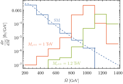
Figure 4: M¯\overline{M} distribution for the SM and new physics contributions. The dashed line shows the fit of the background and for the signal fℛ=0.1f_{\mathcal{R}}=0.1 and a representative C¯ϕ​ℛ​𝒟=0.3\bar{C}_{\phi\mathcal{R}\mathcal{D}}=0.3 was used with the remaining BSMEFT WCs set to zero. The mass of the singly charged scalar is set to 480480 (500500) GeV for the scenario with Mr±⁣±=1M_{r^{\pm\pm}}=1 TeV (Mr±⁣±=1.2M_{r^{\pm\pm}}=1.2 TeV).

III.3 Direct LHC sensitivity to doubly charged scalars

The scalars of Sec. II can be produced at colliders via their hypercharge quantum numbers, implying a predominant production in pairs via Drell-Yan like processes, which is common to many charged scalar extensions of the SM (see e.g. Boos and Volobuev 2018; Bergeaas Kuutmann 2017; Han et al. 2007). The production of two r±⁣±r^{\pm\pm} is more efficient than pair production of h±h^{\pm} due to its larger charge when assuming similar masses. It will also dominate over r±⁣±​r∗r^{\pm\pm}r^{\ast} along with r∗→h∓​h∓r^{\ast}\to h^{\mp}h^{\mp} though a virtual r∗r^{*}, see Ref. Nebot et al. 2008. The r±⁣±r^{\pm\pm} decay phenomenology that we will consider in more detail in this section is characterised by decays r±⁣±→h±​h±r^{\pm\pm}\to h^{\pm}h^{\pm} (when kinematically accessible)

Γ⁡(r±⁣±→h±​h±)=β128​π​Mr±⁣±×{2​𝒞rΛ​v2+m⁡(𝒞ϕ​ℛ​𝒟Λ2​v2+2​𝒞ϕ​𝒮​𝒟Λ2​v2−4)}2,\Gamma(r^{\pm\pm}\to h^{\pm}h^{\pm})={\beta\over 128\pi M_{r^{\pm\pm}}}\\ \times\left\{2{{\cal{C}}_{r}\over\Lambda}\,v^{2}+m\left({{\cal{C}}_{\phi\mathcal{R}\mathcal{D}}\over\Lambda^{2}}\,v^{2}+2\,{{\cal{C}}_{\phi\mathcal{S}\mathcal{D}}\over\Lambda^{2}}\,v^{2}-4\right)\right\}^{2}\,, (19)

where β\beta is the h±h^{\pm} velocity in the r±⁣±r^{\pm\pm} rest frame, as well as same sign lepton decays, e.g.

Γ⁡(r±⁣±→μ±​μ±)=Mr±⁣±128​π×{(4​fℛ,μ​μ−[2​Ce​ℛ​ϕ+fℛ,μ​μ​𝒞ϕ​ℛ​𝒟]​v2Λ2)2+4​Cl​ϕ​ℛ2Λ4​v2}\Gamma(r^{\pm\pm}\to\mu^{\pm}\mu^{\pm})={M_{r^{\pm\pm}}\over 128\pi}\\ \times\left\{\left(4f_{\mathcal{R},\mu\mu}-\left[2\,C_{e\mathcal{R}\phi}+f_{\mathcal{R},\mu\mu}{\cal{C}}_{\phi\mathcal{R}\mathcal{D}}\right]{v^{2}\over\Lambda^{2}}\right)^{2}+4\,{C_{l\phi\mathcal{R}}^{2}\over\Lambda^{4}}\,v^{2}\right\} (20)

in the limit me+≪Mr±⁣±m_{e^{+}}\ll M_{r^{\pm\pm}}. This extends the results of, e.g. Ref. Herrero-Garcia et al. 2014 to EFT interactions. These results can be straightforwardly linearised in ∼1/Λ2\sim 1/\Lambda^{2}.

In the Zee-Babu model, pair production of the doubly-charged scalar through Drell-Yan p​p→Z/A→r+⁣+​r−⁣−pp\to Z/A\to r^{++}r^{--} is only affected by the values of SM couplings and any change in production rate arises through BSMEFT operators. Focusing on the overlap of contributing operators between Drell-Yan, Higgs decays and anomalous muon magnetic moment, we note that only 𝒪ϕ​ℛ​𝒟\mathcal{O}_{\phi\mathcal{R}\mathcal{D}} contributes in the r±⁣±r^{\pm\pm} pair production through a rescaling of the rr field. Considering the possible subsequent decays with leptonic final states we anticipate that the experimental sensitivity of channels with decays to h±h^{\pm} will be significantly impacted by the presence of neutrinos that appear as missing energy. Additionally, any final state involving tau leptons will yield a decreased sensitivity due to the difficulty in tagging them in detectors compared to muons and electrons. In contrast, the four lepton channel r+⁣+​r−⁣−→ℓ+​ℓ+​ℓ−​ℓ−r^{++}r^{--}\to\ell^{+}\ell^{+}\ell^{-}\ell^{-} will provide a clear signature with a suppressed SM background when the fact that r±⁣±r^{\pm\pm} is the only particle in the model decaying to same-charge leptons is exploited in the analysis.

We model the new physics interactions using FeynRules Christensen and Duhr 2009; Alloul et al. 2014 and exporting them in the Ufo Degrande et al. 2012 format that can be imported in MadGraph Alwall et al. 2014. Events for the Zee-Babu and BSMEFT are generated with MadEvent Alwall et al. 2011; de Aquino et al. 2012; Alwall et al. 2014 including only the interference effects of 𝒪ϕ​ℛ​𝒟\mathcal{O}_{\phi\mathcal{R}\mathcal{D}}. We include all SM processes contributing to p​p→ℓ+​ℓ−​ℓ+​ℓ−pp\to\ell^{+}\ell^{-}\ell^{+}\ell^{-} as background with a generation-level cut vetoing events in the MZ±3.5​ΓZM_{Z}\pm 3.5\,\Gamma_{Z} interval, where MZM_{Z} and ΓZ\Gamma_{Z} are the invariant mass and decay width of the (virtual) ZZ boson, respectively. Total decay widths for the charged scalars are calculated with MadWidth Alwall et al. 2015, and cross checked against our analytical results. The events are generated with a fixed branching ratio BR​(r±⁣±→ℓ±​ℓ±)\text{BR}(r^{\pm\pm}\to\ell^{\pm}\ell^{\pm}) and we subsequently rescale the rates under the assumption of the NWA.

Figure 5: Diagram depicting BSMEFT operators that contribute to three measurements considered in the calculation. 𝒪r,𝒪ϕ​ℛ,𝒪ϕ​𝒮,𝒪𝒢​ℛ,𝒪𝒢~​ℛ,𝒪𝒢​𝒮,𝒪𝒢~​𝒮\mathcal{O}_{r},\mathcal{O}_{\phi\mathcal{R}},\mathcal{O}_{\phi\mathcal{S}},\mathcal{O}_{\mathcal{G}\mathcal{R}},\mathcal{O}_{\widetilde{\mathcal{G}}\mathcal{R}},\mathcal{O}_{\mathcal{G}\mathcal{S}},\mathcal{O}_{\widetilde{\mathcal{G}}\mathcal{S}} are the common operators contributing to both Higgs-decay and processes relevant for direct detection for production and decay for charged scalars. 𝒪ℛ​l​e,𝒪𝒮​l​e,𝒪l​ϕ​𝒮,𝒪l​ϕ​ℛ,𝒪e​ℛ​ϕ\mathcal{O}_{\mathcal{R}le},\mathcal{O}_{\mathcal{S}le},\mathcal{O}_{l\phi\mathcal{S}},\mathcal{O}_{l\phi\mathcal{R}},\mathcal{O}_{e\mathcal{R}\phi} contribute to anomalous muon magnetic moment as well as charged scalar production and decay processes. 𝒪ϕ​ℛ​𝒟,𝒪ϕ​𝒮​𝒟\mathcal{O}_{\phi\mathcal{R}\mathcal{D}},\mathcal{O}_{\phi\mathcal{S}\mathcal{D}} contribute to all three processes. A range of the operators are mass-suppressed thus leading to a small overlap in the limit of vanishing quark/lepton masses (e.g. when considering the parton model of LHC collisions).

Our analysis is based on the ATLAS search for doubly charged scalars in Ref. Aaboud et al. 2018 with relaxed cuts and is performed at parton-level to obtain a qualitative, proof-of-principle comparison. Selection of our analysis requires that all light leptons are in the central part of the detector (|η⁡(ℓ)|<2.5\lvert\eta(\ell)\rvert<2.5) with a transverse momentum of pT​(ℓ)>30p_{T}(\ell)>30 GeV. Only leptons with no jet activity within the cone radius Δ​R​(j,ℓ)=Δ​η2+Δ​ϕ<0.4\Delta R(j,\ell)=\sqrt{\Delta\eta^{2}+\Delta\phi}<0.4 are considered and we require exactly four leptons with one positively-charged pair and one negatively-charged, otherwise the event is vetoed (we do not include charge mis-tagging or other experimental systematic uncertainties). A cut is imposed on the invariant mass of each pair such that mℓ±​ℓ±>200m_{\ell^{\pm}\ell^{\pm}}>200 GeV always. Since the same-charged leptons must be a result of r±⁣±r^{\pm\pm} decays we check the consistency of the two masses by calculating

M¯=mℓ+​ℓ++mℓ−​ℓ−2,\overline{M}={m_{\ell^{+}\ell^{+}}+m_{\ell^{-}\ell^{-}}\over 2}\,, (21)

and

Δ​M=|mℓ+​ℓ+−mℓ−​ℓ−|.\Delta M=\lvert m_{\ell^{+}\ell^{+}}-m_{\ell^{-}\ell^{-}}\rvert\,. (22)

The two invariant masses are considered consistent if Δ​M/M¯<0.25\Delta M/\overline{M}<0.25 is satisfied, thus imposing the resonant signal character. Finally, the event is vetoed if a same-flavour, oppositely-charged pair exists with invariant mass in the interval mℓ+​ℓ−∈[81.2,101.2]m_{\ell^{+}\ell^{-}}\in\left[81.2,101.2\right] GeV in order to suppress any background resulting from decays of ZZ bosons.

We evaluate the sensitivity of LHC using events measure from the M¯\overline{M} differential distribution. Including the new physics contributions, the distribution is given by

d​σd​M¯=d​σSMd​M¯+d​σBZd​M¯+𝒞ϕ​ℛ​𝒟Λ2​d​σϕ​ℛ​𝒟d​M¯,\frac{\text{d}\sigma}{\text{d}\overline{M}}=\frac{\text{d}\sigma_{\text{SM}}}{\text{d}\overline{M}}+\frac{\text{d}\sigma_{\text{BZ}}}{\text{d}\overline{M}}+\frac{\mathcal{C}_{\phi\mathcal{R}\mathcal{D}}}{\Lambda^{2}}\frac{\text{d}\sigma_{\phi\mathcal{R}\mathcal{D}}}{\text{d}\overline{M}}\;, (23)

where σSM\sigma_{\text{SM}} denotes the Standard Model contribution and σBZ=σBZ​(fℛ,Mr±⁣±,Mh±)\sigma_{\text{BZ}}=\sigma_{\text{BZ}}(f_{\mathcal{R}},M_{r^{\pm\pm}},M_{h^{\pm}}) the pure Zee-Babu, which depends on the fℛf_{\mathcal{R}} coupling and the masses of r±⁣±r^{\pm\pm} and h±h^{\pm}. The dimension-6 interference contribution from 𝒪ϕ​ℛ​𝒟\mathcal{O}_{\phi\mathcal{R}\mathcal{D}} is denoted as σϕ​ℛ​𝒟\sigma_{\phi\mathcal{R}\mathcal{D}} and also depends on the same parameters as σBZ\sigma_{\text{BZ}}. The new physics contributions are rescaled with a K-factor value of 1.31.3 (see e.g. Altarelli et al. 1979) to include higher order corrections. We note that the dependence on fℛf_{\mathcal{R}} and Mh±M_{h}^{\pm} enters through the branching ratio BR​(r±⁣±→ℓ±​ℓ±)\text{BR}(r^{\pm\pm}\to\ell^{\pm}\ell^{\pm}) and the ratio’s dependence on 𝒞ϕ​ℛ​𝒟\mathcal{C}_{\phi\mathcal{R}\mathcal{D}} cancels out when no other BSMEFT operator is included. This allows us to obtain contributions for different values of fℛf_{\mathcal{R}} by rescaling assuming the NWA and to generate events for interference effects caused by 𝒪ϕ​ℛ​𝒟\mathcal{O}_{\phi\mathcal{R}\mathcal{D}} independent of 𝒞ϕ​ℛ​𝒟\mathcal{C}_{\phi\mathcal{R}\mathcal{D}}.

The M¯\overline{M} distribution obtained from SM processes is fitted away from the signal region to obtain an experimentally-driven estimate for the background for large values of M¯\overline{M}. The M¯\overline{M} distribution for particular values of new physics parameters is shown in Fig. 4. We evaluate the signal and background number of events in the region M¯>200\overline{M}>200 GeV at an integrated luminosity of 33/ab as SS and BB, respectively and calculate, the significance S/BS/\sqrt{B} (S/S+BS/\sqrt{S+B}) under the SM (new physics) hypothesis. We will comment on the search’s sensitivity in the next section.

IV BSMEFT Interplay

We are now ready to consider the phenomenological interplay of the observables discussed in the previous Sec. III.∥∥ ∥ As indicated by the renormalisation procedure, the measurements considered in this work would be part of the input data in comprehensive global fit. In this work we limit ourselves to the phenomenological interplay of the three measurement methodologies assuming vanishing SMEFT contributions. In Fig. 5, the Venn diagram shows the common operators contributing to all three processes discussed in Sec. III. A number of these operators contribute in a fermion mass-suppressed way. The dominant overlap of Higgs data, aμa_{\mu} and Drell-Yan production is therefore a single operator ∼𝒞ϕ​ℛ​𝒟\sim\mathcal{C}_{\phi\mathcal{R}\mathcal{D}}, which only affects the total with of the exotic scalar search. It is worthwhile to stress that when we do not consider effective interactions related to h±h^{\pm}, the anomalous magnetic moment is predictive at 𝒪⁡(Λ−2){\cal{O}}(\Lambda^{-2}), i.e. the r±⁣±r^{\pm\pm} contribution to Δ​a\Delta a is finite even when EFT insertions are considered (see Eq. (15)). The interplay of Higgs data, direct sensitivity in LHC searches and anomalous magnetic moment is therefore relatively transparent in the scenario of Sec. II.

(a)
(b)
Figure 6: Regions in the fℛf_{\mathcal{R}}-𝒞¯ϕ​ℛ​𝒟\bar{\mathcal{C}}_{\phi\mathcal{R}\mathcal{D}} plane, where 𝒞¯i=𝒞i​v2/Λ2\bar{\mathcal{C}}_{i}=\mathcal{C}_{i}v^{2}/\Lambda^{2}. Blue and red show the parameter regions where aμa_{\mu} is in agreement with the Fermilab experimental measurement and the SM expectation, respectively. On the left figure we set Mr±⁣±=1M_{r^{\pm\pm}}=1 TeV and Mh±=0.48M_{h^{\pm}}=0.48 TeV and also show the S/B=3S/\sqrt{B}=3 (S/S+B=3S/\sqrt{S+B}=3) contour for the direct detection analysis with yellow (green) using a value of m=246m=246 GeV. Note that strong EFT coupling (BSMEFT >> BSM) is |C¯ϕ​ℛ​𝒟|≳0.8|{\bar{C}}_{\phi\mathcal{R}\mathcal{D}}|\gtrsim 0.8. On the right, we restrict 𝒞¯ϕ​𝒮​𝒟≈−4​𝒞¯ϕ​ℛ​𝒟\bar{\mathcal{C}}_{\phi\mathcal{S}\mathcal{D}}\approx-4\bar{\mathcal{C}}_{\phi\mathcal{R}\mathcal{D}} and set Mr±⁣±=Mh±=1M_{r^{\pm\pm}}=M_{h^{\pm}}=1 TeV. The contours from the anomalous magnetic moment depend on f𝒮f_{\mathcal{S}} with blue and red contours shown with a value of zero. We note that any value of f𝒮f_{\mathcal{S}} smaller than unity does not significantly affect the results. Additionally, we show the contours that yield agreement with the Fermilab measurement when f𝒮=2f_{\mathcal{S}}=2 with green and overlay the results for the Higgs decay sensitivity from Eq. (17) for the choice of Eq. (25).

In Fig. 6, we show the interplay of the direct search outlined in Sec. III.3 with the anomalous magnetic moment for a particular mass choice of the exotic charged scalars (including open decays r±⁣±→h±​h±r^{\pm\pm}\to h^{\pm}h^{\pm}). The blue contour refers to the Fermilab aμa_{\mu} measurement while the red contour shows the SM expectation as provided in Ref. Aoyama et al. 2020

aμ​(SM)=(116591810±43)×10−11,a_{\mu}(\text{SM})=(116591810\pm 43)\times 10^{-11}\;, (24)

when the uncertainty is used as a limit for new physics. The size of the Fermilab/BNL excess can be compensated by contributions that can be attributed to new BSM physics, overcoming the limitations of the renormalisable Zee-Babu model, however, at strong coupling 𝒞ϕ​ℛ​𝒟​TeV2/Λ2≃66\mathcal{C}_{\phi\mathcal{R}\mathcal{D}}{\text{TeV}^{2}/\Lambda^{2}}\simeq 66. This is due to the fact that the EFT contribution, whilst not being logarithmically enhanced has to overcome the renormalisable contribution of the charged scalars. As already alluded to in Sec. III.1, this can be mitigated by considering charged scalar contributions. Our r±⁣±r^{\pm\pm}-related findings are qualitatively similar to results reported in other model-specific aμa_{\mu} analyses Baer et al. 2021; Athron et al. 2021; Frank et al. 2021; Ellis et al. 2021; Zhang 2021; Jueid et al. 2021; Altmannshofer et al. 2021; Chakraborti et al. 2021a; Chakraborti et al. 2021b: BSM states are forced to be light and/or strongly coupled to address the aμa_{\mu} anomaly. Including signal extrapolations at the LHC as shown in Fig. 6(a) shows that any evidence for new doubly charged states at the LHC would stand in stark contrast with the aμa_{\mu} measurement when interpreted from an extended Zee-Babu perspective.

Including Higgs physics (which is dominated by μg​gγ​γ\mu^{\gamma\gamma}_{gg}) leads to further tension. Even when direct renormalisable trilinear H−r+⁣+−r−⁣−H-r^{++}-r^{--} couplings are dialled small λ5≃0\lambda_{5}\simeq 0 (note that Eq. (8) includes this limit), 𝒪ϕ​ℛ​𝒟\mathcal{O}_{\phi\mathcal{R}\mathcal{D}} (see Tab. 1) introduces the r±⁣±r^{\pm\pm} loop contributions to the Higgs signal strength μg​gγ​γ\mu^{\gamma\gamma}_{gg}, which at this point in the LHC programme is already constrained at the 10% level. Scanning the Higgs signal strength modifications, including the h±h^{\pm} interactions and their dimension-6 EFT modifications, we are not able to reconcile SM consistency of the H→γ​γH\to\gamma\gamma branching with the aμa_{\mu} anomaly when the latter is attributed to choices in the fℛ−𝒞ϕ​ℛ​𝒟f_{\mathcal{R}}-{\mathcal{C}}_{\phi\mathcal{R}\mathcal{D}} plane.

Opening up the EFT and renormalisable coupling space, cancellations between the charged states and their EFT interactions can appear. This typically requires the full renormalisation of aμa_{\mu} as described above. For

𝒞ϕ​𝒮​𝒟=−4​𝒞ϕ​ℛ​𝒟,Mr±⁣±≃Ms±,\mathcal{C}_{\phi\mathcal{S}\mathcal{D}}=-4\,\mathcal{C}_{\phi\mathcal{R}\mathcal{D}},~M_{r^{\pm\pm}}\simeq M_{s^{\pm}}\;, (25)

the charged Higgs contributions cancel. The aμa_{\mu} excess could then be capture in a mismatch of the Yukawa couplings, see Fig. 6(b) We find that fℛ∼5f_{\mathcal{R}}\sim 5 and f𝒮∼1f_{\mathcal{S}}\sim 1 can accommodate the Fermilab excess for strong coupling 𝒞¯ϕ​ℛ​𝒟∼3\bar{\mathcal{C}}_{\phi\mathcal{R}\mathcal{D}}\sim 3, which implies a r±⁣±r^{\pm\pm} partial width into a single lepton combination of around 60​GeV60~\text{GeV}. Such a state can fall into the LHC kinematic coverage, see Fig. 6(a) and Ref. Aaboud et al. 2018. The further exploration of the high mass doubly charged scalar production is therefore highly motivated in the light of a SM-like Higgs and the consolidated aμa_{\mu} anomaly.

V Conclusions

The recent Fermilab consolidation of aμa_{\mu} raises the question of how new physics can be accommodated as the exotics and Higgs precision programme is evolving at the LHC. The direct sensitivity at the LHC with its so far null results in BSM searches moves new physics scales into regions where it becomes challenging to accommodate a significant anomalous magnetic moment of the muon when we take the BNL/Fermilab results as indication for BSM interactions. In this work we have approached the interplay of these experimental arenas by means of effective field theory. A significant muon magnetic moment requires the presence of relatively light charged degrees of freedom which we supplement with a complete dimension-5 and -6 effective field theory analysis. The Zee-Babu scenario as a particularly motivated BSM candidate theory gives then rise to a range of BSMEFT interactions that enable us to discuss aμa_{\mu} precision results in tension with expected developments at the LHC.

Obviously, the rather large number of relevant Wilson coefficients exceed the number of measurements that result from Higgs physics, aμa_{\mu} and direct sensitivity via r±⁣±r^{\pm\pm} pair production, yet the overlapping set of operators that simultaneously affects all measurements and searches is relatively small and shows a significant tension when the SM expectation for Higgs physics is considered: Agreement of aμa_{\mu} requires a significant deformation of charged scalar interactions, which in turn highly modify Higgs physics beyond experimentally allowed constraints. While this is particularly pronounced when we limit ourselves to the r±⁣±r^{\pm\pm} state, we find that the additional freedom provided by the EFT extension of the h±h^{\pm} interactions can be exploited to achieve cancellations that render Higgs data compatible with the SM observation whilst obtaining a sizeable aμa_{\mu}, again at relatively large couplings. On the one hand, this provides an important constraint for potential UV completions that the considered scenarios seeks to inform. On the other hand, the associated parameter ranges can be explored by future searches for doubly charged scalar states as done in e.g. Aad et al. 2020. Additional constraints can in principle be resolved in more challenging p​p→2​ℓ/4​ℓ+E̸Tpp\to 2\ell/4\ell+\not{E}_{T} searches, the impact of which we leave for future work.

Acknowledgements.
The work of A, U.B., and J.C. is supported by the Science and Engineering Research Board, Government of India, under the agreement SERB/PHY/2019501 (MATRICS). C.E. is supported by the UK Science and Technology Facilities Council (STFC) under grant ST/T000945/1 and by the IPPP Associateship Scheme. M.S. is supported by the STFC under grant ST/P001246/1. P.S. is funded by an STFC studentship under grant ST/T506102/1.

Appendix A BSM effective operators

Throughout the paper we assume that the charged scalars 𝒮\mathcal{S} and ℛ\mathcal{R} are light enough to be considered as infrared degrees of freedom. Thus after integrating out the new physics at Λ\Lambda, we are left with effective operators that lead to the modifications of SM interactions (i.e. the SMEFT operators), or can alter the existent BSM interactions at the renormalisable level, and are hereby identified as BSMEFT operators.

The general way to capture the effect of all possible such modifications is to construct a complete and exhaustive set of BSMEFT operators at each mass dimension following Bottom-up approach. A number of models where SM is extended by new degrees of freedom have been discussed in Ref. Banerjee et al. 2021.

We generated Warsaw-like operator bases of dimensions-5 and -6 operators for the case of Zee-Babu model with GrIP Banerjee et al. 2020, the explicit structures of these operators have been tabulated below in Tab. 4, 5 and 6. Notably, we obtain a new class of dimension-5 operators Φ5\Phi^{5}, which unlike for the SMEFT case, arise due to possible gauge invariant structures allowed by hypercharge quantum numbers of the charged scalars.

Φ5\Phi^{5}
𝒪r\mathcal{O}_{r} (ϕ†​ϕ)​𝓡†​𝓢𝟐\boldsymbol{(\phi^{\dagger}\,\phi)\,\mathcal{R}^{\dagger}\,\mathcal{S}^{2}} 𝒪s​r\mathcal{O}_{sr} (𝓢†​𝓢)​𝓡†​𝓢𝟐\boldsymbol{(\mathcal{S}^{\dagger}\,\mathcal{S})\,\mathcal{R}^{\dagger}\,\mathcal{S}^{2}}
𝒪r​s\mathcal{O}_{rs} (𝓡†​𝓡)​𝓡†​𝓢𝟐\boldsymbol{(\mathcal{R}^{\dagger}\,\mathcal{R})\,\mathcal{R}^{\dagger}\,\mathcal{S}^{2}}
Ψ2​Φ2\Psi^{2}\Phi^{2}
𝒪~d​q​ϕ​𝒮\tilde{\mathcal{O}}_{dq\phi\mathcal{S}} (𝑸¯​𝒅)​(ϕ~​𝓢)\boldsymbol{(\overline{Q}\,d)\,(\tilde{\phi}\,\mathcal{S})} 𝒪~u​q​ϕ​𝒮\tilde{\mathcal{O}}_{uq\phi\mathcal{S}} (𝑸¯​𝒖)​(ϕ​𝓢)\boldsymbol{(\overline{Q}\,u)\,(\phi\,\mathcal{S})}
𝒪~l​e​ϕ​𝒮\tilde{\mathcal{O}}_{le\phi\mathcal{S}} (𝑳¯​𝒆)​(ϕ~​𝓢)\boldsymbol{(\overline{L}\,e)\,(\tilde{\phi}\,\mathcal{S})} 𝒪~e​𝒮\tilde{\mathcal{O}}_{e\mathcal{S}} (𝒆𝒄¯​𝒆)​𝓢𝟐\boldsymbol{(\overline{e^{c}}\,e)\,\mathcal{S}^{2}}
Table 4: Explicit structures of the dimension-5 effective operators for the Zee-Babu model. The operators written in bold have distinct hermitian conjugates.
Φ6\Phi^{6} Φ4​𝒟2\Phi^{4}\mathcal{D}^{2}
𝒪𝒮\mathcal{O}_{\mathcal{S}} (𝒮†​𝒮)3(\mathcal{S}^{\dagger}\,\mathcal{S})^{3} 𝒪𝒮​□\mathcal{O}_{\mathcal{S}\square} (𝒮†​𝒮)​□​(𝒮†​𝒮)(\mathcal{S}^{\dagger}\,\mathcal{S})\,\square\,(\mathcal{S}^{\dagger}\,\mathcal{S})
𝒪𝒮​ϕ\mathcal{O}_{\mathcal{S}\phi} (ϕ†​ϕ)​(𝒮†​𝒮)2(\phi^{\dagger}\,\phi)\,(\mathcal{S}^{\dagger}\,\mathcal{S})^{2} 𝒪𝒮​ϕ​𝒟\mathcal{O}_{\mathcal{S}\phi\mathcal{D}} (𝒮†​𝒮)​[(𝒟μ​ϕ)†​(𝒟μ​ϕ)](\mathcal{S}^{\dagger}\,\mathcal{S})\,\left[(\mathcal{D}^{\mu}\,\phi)^{\dagger}(\mathcal{D}_{\mu}\,\phi)\right]
𝒪ϕ​𝒮\mathcal{O}_{\phi\mathcal{S}} (ϕ†​ϕ)2​(𝒮†​𝒮)(\phi^{\dagger}\,\phi)^{2}\,(\mathcal{S}^{\dagger}\,\mathcal{S}) 𝒪ϕ​𝒮​𝒟\mathcal{O}_{\phi\mathcal{S}\mathcal{D}} (ϕ†​ϕ)​[(𝒟μ​𝒮)†​(𝒟μ​𝒮)](\phi^{\dagger}\,\phi)\,\left[(\mathcal{D}^{\mu}\,\mathcal{S})^{\dagger}(\mathcal{D}_{\mu}\,\mathcal{S})\right]
𝒪ℛ\mathcal{O}_{\mathcal{R}} (ℛ†​ℛ)3(\mathcal{R}^{\dagger}\,\mathcal{R})^{3} 𝒪ℛ​□\mathcal{O}_{\mathcal{R}\square} (ℛ†​ℛ)​□​(ℛ†​ℛ)(\mathcal{R}^{\dagger}\,\mathcal{R})\,\square\,(\mathcal{R}^{\dagger}\,\mathcal{R})
𝒪ℛ​ϕ\mathcal{O}_{\mathcal{R}\phi} (ϕ†​ϕ)​(ℛ†​ℛ)2(\phi^{\dagger}\,\phi)\,(\mathcal{R}^{\dagger}\,\mathcal{R})^{2} 𝒪ℛ​ϕ​𝒟\mathcal{O}_{\mathcal{R}\phi\mathcal{D}} (ℛ†​ℛ)​[(𝒟μ​ϕ)†​(𝒟μ​ϕ)](\mathcal{R}^{\dagger}\,\mathcal{R})\,\left[(\mathcal{D}^{\mu}\,\phi)^{\dagger}(\mathcal{D}_{\mu}\,\phi)\right]
𝒪ϕ​ℛ\mathcal{O}_{\phi\mathcal{R}} (ϕ†​ϕ)2​(ℛ†​ℛ)(\phi^{\dagger}\,\phi)^{2}\,(\mathcal{R}^{\dagger}\,\mathcal{R}) 𝒪ϕ​ℛ​𝒟\mathcal{O}_{\phi\mathcal{R}\mathcal{D}} (ϕ†​ϕ)​[(𝒟μ​ℛ)†​(𝒟μ​ℛ)](\phi^{\dagger}\,\phi)\,\left[(\mathcal{D}^{\mu}\,\mathcal{R})^{\dagger}(\mathcal{D}_{\mu}\,\mathcal{R})\right]
𝒪ϕ​ℛ​𝒮\mathcal{O}_{\phi\mathcal{R}\mathcal{S}} (ϕ†​ϕ)​(ℛ†​ℛ)​(𝒮†​𝒮)(\phi^{\dagger}\,\phi)\,(\mathcal{R}^{\dagger}\,\mathcal{R})\,(\mathcal{S}^{\dagger}\,\mathcal{S}) 𝒪𝒮​ℛ​𝒟\mathcal{O}_{\mathcal{S}\mathcal{R}\mathcal{D}} (𝒮†​𝒮)​[(𝒟μ​ℛ)†​(𝒟μ​ℛ)](\mathcal{S}^{\dagger}\,\mathcal{S})\,\left[(\mathcal{D}^{\mu}\,\mathcal{R})^{\dagger}(\mathcal{D}_{\mu}\,\mathcal{R})\right]
𝒪𝒮​ℛ\mathcal{O}_{\mathcal{S}\mathcal{R}} (𝒮†​𝒮)2​(ℛ†​ℛ)(\mathcal{S}^{\dagger}\,\mathcal{S})^{2}\,(\mathcal{R}^{\dagger}\,\mathcal{R}) 𝒪ℛ​𝒮​𝒟\mathcal{O}_{\mathcal{R}\mathcal{S}\mathcal{D}} (ℛ†​ℛ)​[(𝒟μ​𝒮)†​(𝒟μ​𝒮)](\mathcal{R}^{\dagger}\,\mathcal{R})\,\left[(\mathcal{D}^{\mu}\,\mathcal{S})^{\dagger}(\mathcal{D}_{\mu}\,\mathcal{S})\right]
𝒪ℛ​𝒮\mathcal{O}_{\mathcal{R}\mathcal{S}} (𝒮†​𝒮)​(ℛ†​ℛ)2(\mathcal{S}^{\dagger}\,\mathcal{S})\,(\mathcal{R}^{\dagger}\,\mathcal{R})^{2} 𝒪ϕ​𝒮​ℛ​𝒟\mathcal{O}_{\phi\mathcal{S}\mathcal{R}\mathcal{D}} (𝓢†​𝓡)​[(𝓓𝝁​ϕ~†)​(𝓓𝝁​ϕ~)]\boldsymbol{(\mathcal{S}^{\dagger}\,\mathcal{R})\,\left[(\mathcal{D}^{\mu}\,\tilde{\phi}^{\dagger})(\mathcal{D}_{\mu}\,\tilde{\phi})\right]}
𝒪𝒮2​ℛ\mathcal{O}_{\mathcal{S}^{2}\mathcal{R}} (𝓢​𝓡†​𝓢)𝟐\boldsymbol{(\mathcal{S}\,\mathcal{R}^{\dagger}\,\mathcal{S})^{2}}
Φ2​X2\Phi^{2}X^{2} Ψ2​Φ2​𝒟\Psi^{2}\Phi^{2}\mathcal{D}
𝒪B​𝒮\mathcal{O}_{B\mathcal{S}} Bμ​ν​Bμ​ν​(𝒮†​𝒮)B_{\mu\nu}\,B^{\mu\nu}\,(\mathcal{S}^{\dagger}\,\mathcal{S}) 𝒪𝒮​q\mathcal{O}_{\mathcal{S}q} (Q¯​γμ​Q)​(𝒮†​i​𝒟↔μ​𝒮)(\,\overline{Q}\,\gamma^{\mu}\,Q)\,(\mathcal{S}^{\dagger}\,i\overleftrightarrow{\mathcal{D}}_{\mu}\,\mathcal{S})
𝒪B​ℛ\mathcal{O}_{B\mathcal{R}} Bμ​ν​Bμ​ν​(ℛ†​ℛ)B_{\mu\nu}\,B^{\mu\nu}\,(\mathcal{R}^{\dagger}\,\mathcal{R}) 𝒪ℛ​q\mathcal{O}_{\mathcal{R}q} (Q¯​γμ​Q)​(ℛ†​i​𝒟↔μ​ℛ)(\overline{Q}\,\gamma^{\mu}\,Q)\,(\mathcal{R}^{\dagger}\,i\overleftrightarrow{\mathcal{D}}_{\mu}\,\mathcal{R})
𝒪B~​𝒮\mathcal{O}_{\tilde{B}\mathcal{S}} B~μ​ν​Bμ​ν​(𝒮†​𝒮)\tilde{B}_{\mu\nu}\,B^{\mu\nu}\,(\mathcal{S}^{\dagger}\,\mathcal{S}) 𝒪𝒮​l\mathcal{O}_{\mathcal{S}l} (L¯​γμ​L)​(𝒮†​i​𝒟↔μ​𝒮)(\,\overline{L}\,\gamma^{\mu}\,L)\,(\mathcal{S}^{\dagger}\,i\overleftrightarrow{\mathcal{D}}_{\mu}\,\mathcal{S})
𝒪B~​ℛ\mathcal{O}_{\tilde{B}\mathcal{R}} B~μ​ν​Bμ​ν​(ℛ†​ℛ)\tilde{B}_{\mu\nu}\,B^{\mu\nu}\,(\mathcal{R}^{\dagger}\,\mathcal{R}) 𝒪ℛ​l\mathcal{O}_{\mathcal{R}l} (L¯​γμ​L)​(ℛ†​i​𝒟↔μ​ℛ)(\overline{L}\,\gamma^{\mu}\,L)\,(\mathcal{R}^{\dagger}\,i\overleftrightarrow{\mathcal{D}}_{\mu}\,\mathcal{R})
𝒪G​𝒮\mathcal{O}_{G\mathcal{S}} Gμ​νA​GA​μ​ν​(𝒮†​𝒮)G^{A}_{\mu\nu}\,G^{A\mu\nu}\,(\mathcal{S}^{\dagger}\,\mathcal{S}) 𝒪𝒮​u\mathcal{O}_{\mathcal{S}u} (u¯​γμ​u)​(𝒮†​i​𝒟↔μ​𝒮)(\,\overline{u}\,\gamma^{\mu}\,u)\,(\mathcal{S}^{\dagger}\,i\overleftrightarrow{\mathcal{D}}_{\mu}\,\mathcal{S})
𝒪G​ℛ\mathcal{O}_{G\mathcal{R}} Gμ​νA​GA​μ​ν​(ℛ†​ℛ)G^{A}_{\mu\nu}\,G^{A\mu\nu}\,(\mathcal{R}^{\dagger}\,\mathcal{R}) 𝒪ℛ​u\mathcal{O}_{\mathcal{R}u} (u¯​γμ​u)​(ℛ†​i​𝒟↔μ​ℛ)(\overline{u}\,\gamma^{\mu}\,u)\,(\mathcal{R}^{\dagger}\,i\overleftrightarrow{\mathcal{D}}_{\mu}\,\mathcal{R})
𝒪G~​𝒮\mathcal{O}_{\tilde{G}\mathcal{S}} G~μ​νA​GA​μ​ν​(𝒮†​𝒮)\tilde{G}^{A}_{\mu\nu}\,G^{A\mu\nu}\,(\mathcal{S}^{\dagger}\,\mathcal{S}) 𝒪𝒮​d\mathcal{O}_{\mathcal{S}d} (d¯​γμ​d)​(𝒮†​i​𝒟↔μ​𝒮)(\,\overline{d}\,\gamma^{\mu}\,d)\,(\mathcal{S}^{\dagger}\,i\overleftrightarrow{\mathcal{D}}_{\mu}\,\mathcal{S})
𝒪G~​ℛ\mathcal{O}_{\tilde{G}\mathcal{R}} G~μ​νA​GA​μ​ν​(ℛ†​ℛ)\tilde{G}^{A}_{\mu\nu}\,G^{A\mu\nu}\,(\mathcal{R}^{\dagger}\,\mathcal{R}) 𝒪ℛ​d\mathcal{O}_{\mathcal{R}d} (d¯​γμ​d)​(ℛ†​i​𝒟↔μ​ℛ)(\overline{d}\,\gamma^{\mu}\,d)\,(\mathcal{R}^{\dagger}\,i\overleftrightarrow{\mathcal{D}}_{\mu}\,\mathcal{R})
𝒪W​𝒮\mathcal{O}_{W\mathcal{S}} Wμ​νI​WI​μ​ν​(𝒮†​𝒮)W^{I}_{\mu\nu}\,W^{I\mu\nu}\,(\mathcal{S}^{\dagger}\,\mathcal{S}) 𝒪𝒮​e\mathcal{O}_{\mathcal{S}e} (e¯​γμ​e)​(𝒮†​i​𝒟↔μ​𝒮)(\,\overline{e}\,\gamma^{\mu}\,e)\,(\mathcal{S}^{\dagger}\,i\overleftrightarrow{\mathcal{D}}_{\mu}\,\mathcal{S})
𝒪W​ℛ\mathcal{O}_{W\mathcal{R}} Wμ​νI​WI​μ​ν​(ℛ†​ℛ)W^{I}_{\mu\nu}\,W^{I\mu\nu}\,(\mathcal{R}^{\dagger}\,\mathcal{R}) 𝒪ℛ​e\mathcal{O}_{\mathcal{R}e} (e¯​γμ​e)​(ℛ†​i​𝒟↔μ​ℛ)(\overline{e}\,\gamma^{\mu}\,e)\,(\mathcal{R}^{\dagger}\,i\overleftrightarrow{\mathcal{D}}_{\mu}\,\mathcal{R})
𝒪W~​𝒮\mathcal{O}_{\tilde{W}\mathcal{S}} W~μ​νI​WI​μ​ν​(𝒮†​𝒮)\tilde{W}^{I}_{\mu\nu}\,W^{I\mu\nu}\,(\mathcal{S}^{\dagger}\,\mathcal{S}) 𝒪𝒮​l​e\mathcal{O}_{\mathcal{S}le} (𝑳𝒄¯​𝜸𝝁​𝒆)​(ϕ~​𝒊​𝓓𝝁​𝓢)\boldsymbol{(\overline{L^{c}}\,\gamma^{\mu}\,e)(\widetilde{\phi}\,i\mathcal{D}_{\mu}\,\mathcal{S})}
𝒪W~​ℛ\mathcal{O}_{\tilde{W}\mathcal{R}} W~μ​νI​WI​μ​ν​(ℛ†​ℛ)\tilde{W}^{I}_{\mu\nu}\,W^{I\mu\nu}\,(\mathcal{R}^{\dagger}\,\mathcal{R}) 𝒪ℛ​l​e\mathcal{O}_{\mathcal{R}le} (𝑳𝒄¯​𝜸𝝁​𝒆)​(ϕ​𝒊​𝓓𝝁​𝓡)\boldsymbol{(\overline{L^{c}}\,\gamma^{\mu}\,e)(\phi\,i\mathcal{D}_{\mu}\,\mathcal{R})}
Table 5: Explicit structures of the dimension-6 effective operators for the Zee-Babu model. The operators written in bold have distinct hermitian conjugates.
Ψ2​Φ3\Psi^{2}\Phi^{3}
𝒪e​ϕ​𝒮\mathcal{O}_{e\phi\mathcal{S}} (𝑳¯​𝒆)​ϕ​(𝓢†​𝓢)\boldsymbol{(\overline{L}\,e)\,\phi\,(\mathcal{S}^{\dagger}\,\mathcal{S})} 𝒪l​ϕ​𝒮\mathcal{O}_{l\phi\mathcal{S}} (𝑳𝒄¯​𝒊​𝝉𝟐​𝑳)​𝓢​(ϕ†​ϕ)\boldsymbol{(\overline{L^{c}}\,i\tau_{2}\,L)\,\mathcal{S}\,(\phi^{\dagger}\,\phi)}
𝒪u​ϕ​𝒮\mathcal{O}_{u\phi\mathcal{S}} (𝑸¯​𝒖)​ϕ~​(𝓢†​𝓢)\boldsymbol{(\overline{Q}\,u)\,\tilde{\phi}\,(\mathcal{S}^{\dagger}\,\mathcal{S})} 𝒪l​𝒮\mathcal{O}_{l\mathcal{S}} (𝑳𝒄¯​𝒊​𝝉𝟐​𝑳)​𝓢​(𝓢†​𝓢)\boldsymbol{(\overline{L^{c}}\,i\tau_{2}\,L)\,\mathcal{S}\,(\mathcal{S}^{\dagger}\,\mathcal{S})}
𝒪d​ϕ​𝒮\mathcal{O}_{d\phi\mathcal{S}} (𝑸¯​𝒅)​ϕ​(𝓢†​𝓢)\boldsymbol{(\overline{Q}\,d)\,\phi\,(\mathcal{S}^{\dagger}\,\mathcal{S})} 𝒪e​ℛ​ϕ\mathcal{O}_{e\mathcal{R}\phi} (𝒆𝒄¯​𝒆)​𝓡​(ϕ†​ϕ)\boldsymbol{(\overline{e^{c}}\,e)\,\mathcal{R}\,(\phi^{\dagger}\,\phi)}
𝒪e​ϕ​ℛ\mathcal{O}_{e\phi\mathcal{R}} (𝑳¯​𝒆)​ϕ​(𝓡†​𝓡)\boldsymbol{(\overline{L}\,e)\,\phi\,(\mathcal{R}^{\dagger}\,\mathcal{R})} 𝒪l​ϕ​ℛ\mathcal{O}_{l\phi\mathcal{R}} (𝑳𝒄¯​𝒊​𝝉𝟐​𝑳)​(ϕ†​𝓡​ϕ~)\boldsymbol{(\overline{L^{c}}\,i\tau_{2}\,L)\,(\,\phi^{\dagger}\,\mathcal{R}\,\tilde{\phi})}
𝒪u​ϕ​ℛ\mathcal{O}_{u\phi\mathcal{R}} (𝑸¯​𝒖)​ϕ~​(𝓡†​𝓡)\boldsymbol{(\overline{Q}\,u)\,\tilde{\phi}\,(\mathcal{R}^{\dagger}\,\mathcal{R})} 𝒪e​ℛ\mathcal{O}_{e\mathcal{R}} (𝒆𝒄¯​𝒆)​𝓡​(𝓡†​𝓡)\boldsymbol{(\overline{e^{c}}\,e)\,\mathcal{R}\,(\mathcal{R}^{\dagger}\,\mathcal{R})}
𝒪d​ϕ​ℛ\mathcal{O}_{d\phi\mathcal{R}} (𝑸¯​𝒅)​ϕ​(𝓡†​𝓡)\boldsymbol{(\overline{Q}\,d)\,\phi\,(\mathcal{R}^{\dagger}\,\mathcal{R})} 𝒪e​𝒮​ℛ\mathcal{O}_{e\mathcal{S}\mathcal{R}} (𝒆𝒄¯​𝒆)​𝓡​(𝓢†​𝓢)\boldsymbol{(\overline{e^{c}}\,e)\,\mathcal{R}\,(\mathcal{S}^{\dagger}\,\mathcal{S})}
𝒪d​ϕ​ℛ​𝒮\mathcal{O}_{d\phi\mathcal{R}\mathcal{S}} (𝑸¯​𝒅)​ϕ~​(𝓢†​𝓡)\boldsymbol{(\overline{Q}\,d)\,\tilde{\phi}\,(\mathcal{S}^{\dagger}\,\mathcal{R})} 𝒪u​ϕ​ℛ​𝒮\mathcal{O}_{u\phi\mathcal{R}\mathcal{S}} (𝑸¯​𝒖)​ϕ​(𝓡†​𝓢)\boldsymbol{(\overline{Q}\,u)\,\phi\,(\mathcal{R}^{\dagger}\,\mathcal{S})}
Ψ2​Φ​X\Psi^{2}\Phi X
𝒪e​B​𝒮\mathcal{O}_{eB\mathcal{S}} 𝑩𝝁​𝝂​(𝑳𝒄¯​𝝈𝝁​𝝂​𝑳)​𝓢\boldsymbol{B_{\mu\nu}\,(\overline{L^{c}}\,\sigma^{\mu\nu}\,L)\,\mathcal{S}} 𝒪e​W​𝒮\mathcal{O}_{eW\mathcal{S}} 𝑾𝝁​𝝂𝑰​(𝑳𝒄¯​𝝉𝑰​𝝈𝝁​𝝂​𝑳)​𝓢\boldsymbol{W^{I}_{\mu\nu}\,(\overline{L^{c}}\,\tau^{I}\,\sigma^{\mu\nu}\,L)\,\mathcal{S}}
𝒪e​B​ℛ\mathcal{O}_{eB\mathcal{R}} 𝑩𝝁​𝝂​(𝒆𝒄¯​𝝈𝝁​𝝂​𝒆)​𝓡\boldsymbol{B_{\mu\nu}\,(\overline{e^{c}}\,\sigma^{\mu\nu}\,e)\,\mathcal{R}}
Table 6: Explicit structures of the dimension-6 effective operators for the Zee-Babu model. The operators written in bold have distinct hermitian conjugates.

Appendix B Renormalisation

In the following section, we provide the expressions for the renormalisation constants (RC) which we include in the counter terms considered to remove the divergences for the calculation of muon anomalous magnetic moment and Higgs decay to di-photon, as discussed in Sec. III.1 and Sec. III.2 respectively. For both scenarios, we choose on-shell renormalisation for propagating fields and parameters and MS¯\overline{\text{MS}} renormalisation for the Wilson coefficients. The notations used here to express the one-point and the two-point integrals are given along the lines of Ref. Anisha et al. 2021

A0​(m2)=m2​Δ+𝒪⁡(1),B0=Δ+𝒪⁡(1),B1=−Δ2+𝒪⁡(1),B00​(p2,m12,m22)=(m12+m224−p212)​Δ+𝒪⁡(1),\begin{split}A_{0}(m^{2})&=m^{2}\,\Delta+\mathcal{O}(1),\\ B_{0}&=\Delta+\mathcal{O}(1),\\ B_{1}&=-\frac{\Delta}{2}+\mathcal{O}(1),\\ B_{00}(p^{2},m_{1}^{2},m_{2}^{2})&=\left(\frac{m_{1}^{2}+m_{2}^{2}}{4}-\frac{p^{2}}{12}\right)\Delta+\mathcal{O}(1),\end{split}

where Δ\Delta denotes the UV-divergent parts associated with the loop integrals which we remove via the renormalisation of the Wilson coefficients (see e.g. Denner 1993; Denner and Dittmaier 2020. The functions d​BidB_{i} represent the derivative of the scalar functions BiB_{i} with respect to the external momentum. Throughout our work, we express the RCs up to the order of Λ−2\Lambda^{-2} and consistently neglect higher order corrections.

B.1 aμa_{\mu} computation

We evaluate aμa_{\mu} from one-loop μ→μ​γ\mu\to\mu\gamma vertex-function, which requires to consider both δ​ZA​A\delta Z_{AA} and δ​ZZ​A\delta Z_{ZA} wave-function RCs due to the Z−γZ-\gamma mixing. Their explicit expressions computed from on-shell conditions are given as

δ​ZA​A\displaystyle\delta Z_{AA} =[gY2gW224(gY2+gW2)π2+5gY2gW2B0(MW2)16(gY2+gW2)π2\displaystyle=\Big[\frac{g_{{}_{Y}}^{2}g_{{}_{W}}^{2}}{24(g_{{}_{Y}}^{2}+g_{{}_{W}}^{2})\pi^{2}}+\frac{5g_{{}_{Y}}^{2}g_{{}_{W}}^{2}B_{0}(M_{{}_{W}}^{2})}{16(g_{{}_{Y}}^{2}+g_{{}_{W}}^{2})\pi^{2}}
+gY2gW2B1(MW2)8(gY2+gW2)π2+gY2gW2MW2dB0(MW2)8(gY2+gW2)π2\displaystyle+\frac{g_{{}_{Y}}^{2}g_{{}_{W}}^{2}B_{1}(M_{{}_{W}}^{2})}{8(g_{{}_{Y}}^{2}+g_{{}_{W}}^{2})\pi^{2}}+\frac{g_{{}_{Y}}^{2}g_{{}_{W}}^{2}M_{{}_{W}}^{2}\,dB_{0}(M_{{}_{W}}^{2})}{8(g_{{}_{Y}}^{2}+g_{{}_{W}}^{2})\pi^{2}}
−gY2gW4v2dB0(MW2)32(gY2+gW2)π2+gY2gW2dB00(Mr±⁣±2)(gY2+gW2)π2\displaystyle-\frac{g_{{}_{Y}}^{2}g_{{}_{W}}^{4}v^{2}\,dB_{0}(M_{{}_{W}}^{2})}{32(g_{{}_{Y}}^{2}+g_{{}_{W}}^{2})\pi^{2}}+\frac{g_{{}_{Y}}^{2}g_{{}_{W}}^{2}\,dB_{00}(M_{r^{\pm\pm}}^{2})}{(g_{{}_{Y}}^{2}+g_{{}_{W}}^{2})\pi^{2}}
+gY2gW2(dB00(Mh±2)+3dB00(MW2))4(gY2+gW2)π2\displaystyle+\frac{g_{{}_{Y}}^{2}g_{{}_{W}}^{2}\Big(dB_{00}(M_{h^{\pm}}^{2})+3\,dB_{00}(M_{{}_{W}}^{2})\Big)}{4(g_{{}_{Y}}^{2}+g_{{}_{W}}^{2})\pi^{2}}
+∑l=e,μ,τgY2gW2B1(Ml2)4(gY2+gW2)π2+∑qu=u,c,tgY2gW2B1(Mqu2)3(gY2+gW2)π2\displaystyle+\sum_{l=e,\mu,\tau}\frac{g_{{}_{Y}}^{2}g_{{}_{W}}^{2}B_{1}(M_{{}_{l}}^{2})}{4(g_{{}_{Y}}^{2}+g_{{}_{W}}^{2})\pi^{2}}+\sum_{q_{u}=u,c,t}\frac{g_{{}_{Y}}^{2}g_{{}_{W}}^{2}B_{1}(M_{q_{u}}^{2})}{3(g_{{}_{Y}}^{2}+g_{{}_{W}}^{2})\pi^{2}}
+∑qd=d,s,bgY2gW2B1(Mqd2)12(gY2+gW2)π2−∑l=e,μ,τ2gY2gW2dB00(Ml2)2(gY2+gW2)π2\displaystyle+\sum_{q_{d}=d,s,b}\frac{g_{{}_{Y}}^{2}g_{{}_{W}}^{2}B_{1}(M_{q_{d}}^{2})}{12(g_{{}_{Y}}^{2}+g_{{}_{W}}^{2})\pi^{2}}-\sum_{l=e,\mu,\tau}\frac{2g_{{}_{Y}}^{2}g_{{}_{W}}^{2}dB_{00}(M_{{}_{l}}^{2})}{2(g_{{}_{Y}}^{2}+g_{{}_{W}}^{2})\pi^{2}}
−∑qu=u,c,t2gY2gW2dB00(Mqu2)3(gY2+gW2)π2\displaystyle-\sum_{q_{u}=u,c,t}\frac{2g_{{}_{Y}}^{2}g_{{}_{W}}^{2}dB_{00}(M_{q_{u}}^{2})}{3(g_{{}_{Y}}^{2}+g_{{}_{W}}^{2})\pi^{2}}
−∑qd=d,s,bgY2gW2dB00(Mqd2)6(gY2+gW2)π2],\displaystyle-\sum_{q_{d}=d,s,b}\frac{g_{{}_{Y}}^{2}g_{{}_{W}}^{2}dB_{00}(M_{q_{d}}^{2})}{6(g_{{}_{Y}}^{2}+g_{{}_{W}}^{2})\pi^{2}}\Big], (26)

and

δ​ZA​Z\displaystyle\delta Z_{AZ} =[gYgW312(gY2+gW2)π2+gY3gW(4A0(Mr±⁣±2)+A0(Mh±2))4(gY2+gW2)MZ2π2\displaystyle=\Big[\frac{g_{{}_{Y}}g_{{}_{W}}^{3}}{12(g_{{}_{Y}}^{2}+g_{{}_{W}}^{2})\pi^{2}}+\frac{g_{{}_{Y}}^{3}g_{{}_{W}}\Big(4A_{0}(M_{r^{\pm\pm}}^{2})+A_{0}(M_{h^{\pm}}^{2})\Big)}{4(g_{{}_{Y}}^{2}+g_{{}_{W}}^{2})M_{{}_{Z}}^{2}\pi^{2}}
−∑l=e,μ,τgYgW(3gY2A0(Ml2)+gW2A0(Ml2))8(gY2+gW2)MZ2π2\displaystyle-\sum_{l=e,\mu,\tau}\frac{g_{{}_{Y}}g_{{}_{W}}\Big(3g_{{}_{Y}}^{2}A_{0}(M_{{}_{l}}^{2})+g_{{}_{W}}^{2}A_{0}(M_{{}_{l}}^{2})\Big)}{8(g_{{}_{Y}}^{2}+g_{{}_{W}}^{2})M_{{}_{Z}}^{2}\pi^{2}}
+∑qd=d,s,bgYgW(3gW2A0(Mqd2)−gY2A0(Mqd2))24(gY2+gW2)MZ2π2\displaystyle+\sum_{q_{d}=d,s,b}\frac{g_{{}_{Y}}g_{{}_{W}}\Big(3g_{{}_{W}}^{2}A_{0}(M_{q_{d}}^{2})-g_{{}_{Y}}^{2}A_{0}(M_{q_{d}}^{2})\Big)}{24(g_{{}_{Y}}^{2}+g_{{}_{W}}^{2})M_{{}_{Z}}^{2}\pi^{2}}
+∑qu=u,c,tgYgW(3gW2A0(Mqu2)−5gY2A0(Mqu2))12(gY2+gW2)MZ2π2\displaystyle+\sum_{q_{u}=u,c,t}\frac{g_{{}_{Y}}g_{{}_{W}}\Big(3g_{{}_{W}}^{2}A_{0}(M_{q_{u}}^{2})-5g_{{}_{Y}}^{2}A_{0}(M_{q_{u}}^{2})\Big)}{12(g_{{}_{Y}}^{2}+g_{{}_{W}}^{2})M_{{}_{Z}}^{2}\pi^{2}}
+gYgW16(gY2+gW2)MZ2π2B00(MZ2,MW2)(10gW2MZ2\displaystyle+\frac{g_{{}_{Y}}g_{{}_{W}}}{16(g_{{}_{Y}}^{2}+g_{{}_{W}}^{2})M_{{}_{Z}}^{2}\pi^{2}}B_{00}(M_{{}_{Z}}^{2},M_{{}_{W}}^{2})\Big(10g_{{}_{W}}^{2}M_{{}_{Z}}^{2}
+4gW2MW2+gY2gW2v2−4gY2+10gW2)\displaystyle+4g_{{}_{W}}^{2}M_{{}_{W}}^{2}+g_{{}_{Y}}^{2}g_{{}_{W}}^{2}v^{2}-4g_{{}_{Y}}^{2}+10g_{{}_{W}}^{2}\Big)
+gYgW(gY2A0(MW2)−5gW2A0(MW2))8(gY2+gW2)MZ2π2\displaystyle+\frac{g_{{}_{Y}}g_{{}_{W}}\Big(g_{{}_{Y}}^{2}A_{0}(M_{{}_{W}}^{2})-5g_{{}_{W}}^{2}A_{0}(M_{{}_{W}}^{2})\Big)}{8(g_{{}_{Y}}^{2}+g_{{}_{W}}^{2})M_{{}_{Z}}^{2}\pi^{2}}
+gY3gW(B00(MZ2,Mh±2)−4B00(MZ2,Mr±⁣±2))2(gY2+gW2)MZ2π2\displaystyle+\frac{g_{{}_{Y}}^{3}g_{{}_{W}}\Big(B_{00}(M_{{}_{Z}}^{2},M_{h^{\pm}}^{2})-4B_{00}(M_{{}_{Z}}^{2},M_{r^{\pm\pm}}^{2})\Big)}{2(g_{{}_{Y}}^{2}+g_{{}_{W}}^{2})M_{{}_{Z}}^{2}\pi^{2}}
+∑l=e,μ,τgYgW(3gY2−gW2)B00(MZ2,Ml2)4(gY2+gW2)MZ2π2\displaystyle+\sum_{l=e,\mu,\tau}\frac{g_{{}_{Y}}g_{{}_{W}}\Big(3g_{{}_{Y}}^{2}-g_{{}_{W}}^{2}\Big)B_{00}(M_{{}_{Z}}^{2},M_{{}_{l}}^{2})}{4(g_{{}_{Y}}^{2}+g_{{}_{W}}^{2})M_{{}_{Z}}^{2}\pi^{2}}
+∑qd=d,s,bgYgW(gY2−3gW2)B00(MZ2,Mqd2)12(gY2+gW2)MZ2π2\displaystyle+\sum_{q_{d}=d,s,b}\frac{g_{{}_{Y}}g_{{}_{W}}\Big(g_{{}_{Y}}^{2}-3g_{{}_{W}}^{2}\Big)B_{00}(M_{{}_{Z}}^{2},M_{q_{d}}^{2})}{12(g_{{}_{Y}}^{2}+g_{{}_{W}}^{2})M_{{}_{Z}}^{2}\pi^{2}}
+∑qu=u,c,tgYgW(5gY2−3gW2)B00(MZ2,Mqu2)6(gY2+gW2)MZ2π2\displaystyle+\sum_{q_{u}=u,c,t}\frac{g_{{}_{Y}}g_{{}_{W}}\Big(5g_{{}_{Y}}^{2}-3g_{{}_{W}}^{2}\Big)B_{00}(M_{{}_{Z}}^{2},M_{q_{u}}^{2})}{6(g_{{}_{Y}}^{2}+g_{{}_{W}}^{2})M_{{}_{Z}}^{2}\pi^{2}}
+∑f=l,qu,qdgYgW(gW2−3gY2)B1(MZ2,Mf2)8(gY2+gW2)MZ2π2\displaystyle+\sum_{f=l,q_{u},q_{d}}\frac{g_{{}_{Y}}g_{{}_{W}}\Big(g_{{}_{W}}^{2}-3g_{{}_{Y}}^{2}\Big)B_{1}(M_{{}_{Z}}^{2},M_{{}_{f}}^{2})}{8(g_{{}_{Y}}^{2}+g_{{}_{W}}^{2})M_{{}_{Z}}^{2}\pi^{2}}
+gYgW3B1(MZ2,MW2)4(gY2+gW2)π2]+gYgW2(gY2+gW2)π2[\displaystyle+\frac{g_{{}_{Y}}g_{{}_{W}}^{3}B_{1}(M_{Z}^{2},M_{{}_{W}}^{2})}{4(g_{{}_{Y}}^{2}+g_{{}_{W}}^{2})\pi^{2}}\Big]+\frac{g_{{}_{Y}}g_{{}_{W}}}{2(g_{{}_{Y}}^{2}+g_{{}_{W}}^{2})\pi^{2}}\Big[
(𝒞B​ℛ−𝒞W​ℛΛ2)​A0​(Mr±⁣±2)+(𝒞B​𝒮−𝒞W​𝒮Λ2)\displaystyle\Big(\frac{\mathcal{C}_{B\mathcal{R}}-\mathcal{C}_{W\mathcal{R}}}{\Lambda^{2}}\Big)A_{0}(M_{r^{\pm\pm}}^{2})+\Big(\frac{\mathcal{C}_{B\mathcal{S}}-\mathcal{C}_{W\mathcal{S}}}{\Lambda^{2}}\Big)
A0(Mh±2)],\displaystyle A_{0}(M_{h^{\pm}}^{2})\Big], (27)

respectively.

Similarly, we include the wave-function renormalisation for the left and right chiral components of external muon fields

δZfL\displaystyle\delta Z_{f_{{}_{L}}} =[(gY4+4gY2gW2+3gW4)64(gY2+gW2)π2\displaystyle=\Big[\frac{(g_{{}_{Y}}^{4}+4g_{{}_{Y}}^{2}g_{{}_{W}}^{2}+3g_{{}_{W}}^{4})}{64(g_{{}_{Y}}^{2}+g_{{}_{W}}^{2})\pi^{2}}
−fℛ2Mμ2(dB0(Mμ2,,Mr±⁣±2)−dB1(Mμ2,,Mr±⁣±2))4​π2\displaystyle-\frac{f_{\mathcal{R}}^{2}M_{\mu}^{2}(dB_{0}(M_{\mu}^{2},,M_{r^{\pm\pm}}^{2})-dB_{1}(M_{\mu}^{2},,M_{r^{\pm\pm}}^{2}))}{4\pi^{2}}
−f𝒮2​(B0​(Mμ2,Mh±2)−B1​(Mμ2,Mh±2))8​π2\displaystyle-\frac{f_{\mathcal{S}}^{2}\Big(B_{0}(M_{\mu}^{2},M_{h^{\pm}}^{2})-B_{1}(M_{\mu}^{2},M_{h^{\pm}}^{2})\Big)}{8\pi^{2}}
−f𝒮2​Mμ2​(d​B0​(Mμ2,Mh±2)−d​B1​(Mμ2,Mh±2))8​π2\displaystyle-\frac{f_{\mathcal{S}}^{2}M_{\mu}^{2}\Big(dB_{0}(M_{\mu}^{2},M_{h^{\pm}}^{2})-dB_{1}(M_{\mu}^{2},M_{h^{\pm}}^{2})\Big)}{8\pi^{2}}
−gY2gW28(gY2+gW2)π2​(B0​(Mμ2,Mμ2)−B1​(Mμ2,Mμ2)CLOSE\displaystyle-\frac{g_{{}_{Y}}^{2}g_{{}_{W}}^{2}}{8(g_{{}_{Y}}^{2}+g_{{}_{W}}^{2})\pi^{2}}\Big(B_{0}(M_{\mu}^{2},M_{\mu}^{2})-B_{1}(M_{\mu}^{2},M_{\mu}^{2})
OPEN+2​Mμ2​(d​B0​(Mμ2,Mμ2)−d​B1​(Mμ2,Mμ2)))\displaystyle+2M_{\mu}^{2}\Big(dB_{0}(M_{\mu}^{2},M_{\mu}^{2})-dB_{1}(M_{\mu}^{2},M_{\mu}^{2})\Big)\Big)
−gW2(gY2+gW2)(B0(Mμ2,MW2)+B1(Mμ2,MW2))16(gY2+gW2)π2\displaystyle-\frac{g_{{}_{W}}^{2}\Big(g_{{}_{Y}}^{2}+g_{{}_{W}}^{2}\Big)\Big(B_{0}(M_{\mu}^{2},M_{{}_{W}}^{2})+B_{1}(M_{\mu}^{2},M_{{}_{W}}^{2})\Big)}{16(g_{{}_{Y}}^{2}+g_{{}_{W}}^{2})\pi^{2}}
−(gY2−gW2)2(B0(Mμ2,MZ2)+B0(Mμ2,MW2))32(gY2+gW2)π2\displaystyle-\frac{(g_{{}_{Y}}^{2}-g_{{}_{W}}^{2})^{2}\Big(B_{0}(M_{\mu}^{2},M_{{}_{Z}}^{2})+B_{0}(M_{\mu}^{2},M_{{}_{W}}^{2})\Big)}{32(g_{{}_{Y}}^{2}+g_{{}_{W}}^{2})\pi^{2}}
−Mμ2(B0(Mμ2,MH2)−B1(Mμ2,MH2))16​π2​v2\displaystyle-\frac{M_{\mu}^{2}\Big(B_{0}(M_{\mu}^{2},M_{{}_{H}}^{2})-B_{1}(M_{\mu}^{2},M_{{}_{H}}^{2})\Big)}{16\pi^{2}v^{2}}
−Mμ2(B0(Mμ2,MZ2)−B1(Mμ2,MZ2))16​π2​v2\displaystyle-\frac{M_{\mu}^{2}\Big(B_{0}(M_{\mu}^{2},M_{{}_{Z}}^{2})-B_{1}(M_{\mu}^{2},M_{{}_{Z}}^{2})\Big)}{16\pi^{2}v^{2}}
−Mμ48​π2​v2(dB0(Mμ2,MW2)+dB1(Mμ2,MW2)\displaystyle-\frac{M_{\mu}^{4}}{8\pi^{2}v^{2}}\Big(dB_{0}(M_{\mu}^{2},M_{{}_{W}}^{2})+dB_{1}(M_{\mu}^{2},M_{{}_{W}}^{2})
−2dB0(Mμ2,MH2)+dB1(Mμ2,MH2)−dB1(Mμ2,MZ2))]\displaystyle-2dB_{0}(M_{\mu}^{2},M_{{}_{H}}^{2})+dB_{1}(M_{\mu}^{2},M_{{}_{H}}^{2})-dB_{1}(M_{\mu}^{2},M_{{}_{Z}}^{2})\Big)\Big]
+v2​(2​fℛ2​𝒞ϕ​ℛ​𝒟+f𝒮2​𝒞ϕ​𝒮​𝒟+f𝒮​𝒞l​ϕ​𝒮)16​π2​Λ2[\displaystyle+\frac{v^{2}(2f_{\mathcal{R}}^{2}\mathcal{C}_{\phi\mathcal{R}\mathcal{D}}+f_{\mathcal{S}}^{2}\mathcal{C}_{\phi\mathcal{S}\mathcal{D}}+f_{\mathcal{S}}\mathcal{C}_{l\phi\mathcal{S}})}{16\pi^{2}\Lambda^{2}}\Big[
(B0​(Mμ2,Mr±⁣±2)+B1​(Mμ2,Mr±⁣±2))\displaystyle\Big(B_{0}(M_{\mu}^{2},M_{r^{\pm\pm}}^{2})+B_{1}(M_{\mu}^{2},M_{r^{\pm\pm}}^{2})\Big)
+Mμ2(dB0(Mμ2,Mr±⁣±2)+dB1(Mμ2,Mr±⁣±2))]\displaystyle+M_{{}_{\mu}}^{2}\Big(dB_{0}(M_{\mu}^{2},M_{r^{\pm\pm}}^{2})+dB_{1}(M_{\mu}^{2},M_{r^{\pm\pm}}^{2})\Big)\Big]
+Mμ2​v2​fℛ​𝒞e​ℛ​ϕ4​π2​Λ2[(dB0(Mμ2,Mr±⁣±2)\displaystyle+\frac{M_{\mu}^{2}v^{2}f_{\mathcal{R}}\mathcal{C}_{e\mathcal{R}\phi}}{4\pi^{2}\Lambda^{2}}\Big[\Big(dB_{0}(M_{\mu}^{2},M_{r^{\pm\pm}}^{2})
+dB1(Mμ2,Mr±⁣±2))]+fℛ​Mμ2​v2​𝒞l​ϕ​ℛ4​π2​Λ2dB0(Mμ2,Mr±⁣±2)\displaystyle+dB_{1}(M_{\mu}^{2},M_{r^{\pm\pm}}^{2})\Big)\Big]+\frac{f_{\mathcal{R}}M_{\mu}^{2}v^{2}\mathcal{C}_{l\phi\mathcal{R}}}{4\pi^{2}\Lambda^{2}}dB_{0}(M_{\mu}^{2},M_{r^{\pm\pm}}^{2})
+fℛ​Mμ​v​𝒞ℛ​l​e4​2​π2​Λ2[B0(Mμ2,Mr±⁣±2)+B1(Mμ2,Mr±⁣±2)\displaystyle+\frac{f_{\mathcal{R}}M_{\mu}v\,\mathcal{C}_{\mathcal{R}le}}{4\sqrt{2}\pi^{2}\Lambda^{2}}\Big[B_{0}(M_{\mu}^{2},M_{r^{\pm\pm}}^{2})+B_{1}(M_{\mu}^{2},M_{r^{\pm\pm}}^{2})
+2Mμ2dB0(Mμ2,Mr±⁣±2)]+f𝒮​Mμ​v​𝒞𝒮​l​e4​2​π2​Λ2\displaystyle+2\,M_{\mu}^{2}\,dB_{0}(M_{\mu}^{2},M_{r^{\pm\pm}}^{2})\Big]+\frac{f_{\mathcal{S}}M_{\mu}v\,\mathcal{C}_{\mathcal{S}le}}{4\sqrt{2}\pi^{2}\Lambda^{2}}
[B0(Mμ2,Mr±⁣±2)+B1(Mμ2,Mr±⁣±2)\displaystyle\Big[B_{0}(M_{\mu}^{2},M_{r^{\pm\pm}}^{2})+B_{1}(M_{\mu}^{2},M_{r^{\pm\pm}}^{2})
+2Mμ2(dB0(Mμ2,Mr±⁣±2)+dB1(Mμ2,Mr±⁣±2))],\displaystyle+2\,M_{\mu}^{2}\,\Big(dB_{0}(M_{\mu}^{2},M_{r^{\pm\pm}}^{2})+dB_{1}(M_{\mu}^{2},M_{r^{\pm\pm}}^{2})\Big)\Big], (28)

and

δ​ZfR\displaystyle\delta Z_{f_{R}} =[gY216​π2−gY4(B0(MZ2,Mμ2)+B1(MZ2,Mμ2))8(gY2+gW2)π2\displaystyle=\Big[\frac{g_{{}_{Y}}^{2}}{16\pi^{2}}-\frac{g_{{}_{Y}}^{4}\Big(B_{0}(M_{{}_{Z}}^{2},M_{\mu}^{2})+B_{1}(M_{{}_{Z}}^{2},M_{\mu}^{2})\Big)}{8(g_{{}_{Y}}^{2}+g_{{}_{W}}^{2})\pi^{2}}
−fℛ24​π2​(B0​(Mr±⁣±2,Mμ2)+B1​(Mr±⁣±2,Mμ2)CLOSE\displaystyle-\frac{f_{\mathcal{R}}^{2}}{4\pi^{2}}\Big(B_{0}(M_{r^{\pm\pm}}^{2},M_{\mu}^{2})+B_{1}(M_{r^{\pm\pm}}^{2},M_{\mu}^{2})
OPEN+Mμ2​(d​B0​(Mr±⁣±2,Mμ2),d​B1​(Mr±⁣±2,Mμ2)))\displaystyle+M_{\mu}^{2}\Big(dB_{0}(M_{r^{\pm\pm}}^{2},M_{\mu}^{2}),dB_{1}(M_{r^{\pm\pm}}^{2},M_{\mu}^{2})\Big)\Big)
−f𝒮2​Mμ28​π2​(d​B0​(Mh±2,Mμ2)+d​B1​(Mh±2,Mμ2))\displaystyle-\frac{f_{\mathcal{S}}^{2}M_{\mu}^{2}}{8\pi^{2}}\Big(dB_{0}(M_{h^{\pm}}^{2},M_{\mu}^{2})+dB_{1}(M_{h^{\pm}}^{2},M_{\mu}^{2})\Big)
−gY2gW28(gY2+gW2)π2​(B0​(Mμ2,Mμ2)+B1​(Mμ2,Mμ2)CLOSE\displaystyle-\frac{g_{{}_{Y}}^{2}g_{{}_{W}}^{2}}{8(g_{{}_{Y}}^{2}+g_{{}_{W}}^{2})\pi^{2}}\Big(B_{0}(M_{\mu}^{2},M_{\mu}^{2})+B_{1}(M_{\mu}^{2},M_{\mu}^{2})
OPEN−2​(d​B0​(Mμ2,Mμ2)+d​B1​(Mμ2,Mμ2)))\displaystyle-2\Big(dB_{0}(M_{\mu}^{2},M_{\mu}^{2})+dB_{1}(M_{\mu}^{2},M_{\mu}^{2})\Big)\Big)
−Mμ216​π2​v2(2B0(MW2,Mμ2)+B0(Mh±2,Mμ2)\displaystyle-\frac{M_{\mu}^{2}}{16\pi^{2}v^{2}}\Big(2B_{0}(M_{{}_{W}}^{2},M_{\mu}^{2})+B_{0}(M_{h^{\pm}}^{2},M_{\mu}^{2})
+2B1(MW2,Mμ2)+B0(MZ2,Mμ2)−B1(MZ2,Mμ2))\displaystyle+2B_{1}(M_{{}_{W}}^{2},M_{\mu}^{2})+B_{0}(M_{{}_{Z}}^{2},M_{\mu}^{2})-B_{1}(M_{{}_{Z}}^{2},M_{\mu}^{2})\Big)
−Mμ232(gY2+gW2)π2(8gY2gW2dB0(Mμ2,Mμ2)+(3gY4\displaystyle-\frac{M_{\mu}^{2}}{32(g_{{}_{Y}}^{2}+g_{{}_{W}}^{2})\pi^{2}}\Big(8g_{{}_{Y}}^{2}g_{{}_{W}}^{2}dB_{0}(M_{\mu}^{2},M_{\mu}^{2})+(3g_{{}_{Y}}^{4}
−3gY2gW2−gY4)dB0(MZ2,Mμ2)−gY2gW2dB1(Mμ2,Mμ2)\displaystyle-3g_{{}_{Y}}^{2}g_{{}_{W}}^{2}-g_{{}_{Y}}^{4})dB_{0}(M_{{}_{Z}}^{2},M_{\mu}^{2})-g_{{}_{Y}}^{2}g_{{}_{W}}^{2}dB_{1}(M_{\mu}^{2},M_{\mu}^{2})
−(5gY4−2gY2gW2+gW4)dB1(MZ2,Mμ2))−Mμ48​π2​v2\displaystyle-(5g_{{}_{Y}}^{4}-2g_{{}_{Y}}^{2}g_{{}_{W}}^{2}+g_{{}_{W}}^{4})dB_{1}(M_{{}_{Z}}^{2},M_{\mu}^{2})\Big)-\frac{M_{\mu}^{4}}{8\pi^{2}v^{2}}
(dB0(MW2,Mμ2)+2dB0(Mh±2,Mμ2)+dB1(Mh±2,Mμ2)\displaystyle\Big(dB_{0}(M_{{}_{W}}^{2},M_{\mu}^{2})+2dB_{0}(M_{h^{\pm}}^{2},M_{\mu}^{2})+dB_{1}(M_{h^{\pm}}^{2},M_{\mu}^{2})
+dB1(MW2,Mμ2)+dB1(MZ2,Mμ2))]+𝒞ϕ​ℛ​𝒟​fℛ2​v28​π2​Λ2\displaystyle+dB_{1}(M_{{}_{W}}^{2},M_{\mu}^{2})+dB_{1}(M_{{}_{Z}}^{2},M_{\mu}^{2})\Big)\Big]+\frac{\mathcal{C}_{\phi\mathcal{R}\mathcal{D}}f_{\mathcal{R}}^{2}v^{2}}{8\pi^{2}\Lambda^{2}}
[B0(Mh±2,Mμ2)+B1(Mh±2,Mμ2)+Mμ2(dB0(Mh±2,Mμ2)\displaystyle\Big[B_{0}(M_{h^{\pm}}^{2},M_{\mu}^{2})+B_{1}(M_{h^{\pm}}^{2},M_{\mu}^{2})+M_{\mu}^{2}\Big(dB_{0}(M_{h^{\pm}}^{2},M_{\mu}^{2})
dB1(Mh±2,Mμ2))]+𝒞ϕ​𝒮​𝒟​f𝒮2​Mμ2​v216​π2​Λ2[dB0(Mh±2,Mμ2)\displaystyle dB_{1}(M_{h^{\pm}}^{2},M_{\mu}^{2})\Big)\Big]+\frac{\mathcal{C}_{\phi\mathcal{S}\mathcal{D}}f_{\mathcal{S}}^{2}M_{\mu}^{2}v^{2}}{16\pi^{2}\Lambda^{2}}\Big[dB_{0}(M_{h^{\pm}}^{2},M_{\mu}^{2})
+dB1(Mh±2,Mμ2)]+𝒞e​ℛ​ϕ​fℛ​v24​π2​Λ2[B0(Mr±⁣±2,Mμ2)\displaystyle+dB_{1}(M_{h^{\pm}}^{2},M_{\mu}^{2})\Big]+\frac{\mathcal{C}_{e\mathcal{R}\phi}f_{\mathcal{R}}v^{2}}{4\pi^{2}\Lambda^{2}}\Big[B_{0}(M_{r^{\pm\pm}}^{2},M_{\mu}^{2})
+B1​(Mr±⁣±2,Mμ2)+Mμ2​(d​B0​(Mr±⁣±2,Mμ2)CLOSE\displaystyle+B_{1}(M_{r^{\pm\pm}}^{2},M_{\mu}^{2})+M_{\mu}^{2}\Big(dB_{0}(M_{r^{\pm\pm}}^{2},M_{\mu}^{2})
+dB1(Mr±⁣±2,Mμ2))]+𝒞l​ϕ​ℛ​fℛ​Mμ2​v2​d​B0​(Mr±⁣±2,Mμ2)4​π2​Λ2\displaystyle+dB_{1}(M_{r^{\pm\pm}}^{2},M_{\mu}^{2})\Big)\Big]+\frac{\mathcal{C}_{l\phi\mathcal{R}}f_{\mathcal{R}}M_{\mu}^{2}v^{2}dB_{0}(M_{r^{\pm\pm}}^{2},M_{\mu}^{2})}{4\pi^{2}\Lambda^{2}}
+𝒞l​ϕ​𝒮​f𝒮​Mμ2​v216​π2​Λ2​[d​B0​(Mh±2,Mμ2)+d​B1​(Mh±2,Mμ2)]\displaystyle+\frac{\mathcal{C}_{l\phi\mathcal{S}}f_{\mathcal{S}}M_{\mu}^{2}v^{2}}{16\pi^{2}\Lambda^{2}}\Big[dB_{0}(M_{h^{\pm}}^{2},M_{\mu}^{2})+dB_{1}(M_{h^{\pm}}^{2},M_{\mu}^{2})\Big]
+fℛ​Mμ​v​𝒞ℛ​l​e4​2​π2​Λ2[B0(Mμ2,Mr±⁣±2)+B1(Mμ2,Mr±⁣±2)\displaystyle+\frac{f_{\mathcal{R}}M_{\mu}v\,\mathcal{C}_{\mathcal{R}le}}{4\sqrt{2}\pi^{2}\Lambda^{2}}\Big[B_{0}(M_{\mu}^{2},M_{r^{\pm\pm}}^{2})+B_{1}(M_{\mu}^{2},M_{r^{\pm\pm}}^{2})
+2Mμ2dB0(Mμ2,Mr±⁣±2)]+f𝒮​Mμ​v​𝒞𝒮​l​e4​2​π2​Λ2\displaystyle+2\,M_{\mu}^{2}\,dB_{0}(M_{\mu}^{2},M_{r^{\pm\pm}}^{2})\Big]+\frac{f_{\mathcal{S}}M_{\mu}v\,\mathcal{C}_{\mathcal{S}le}}{4\sqrt{2}\pi^{2}\Lambda^{2}}
[B0(Mμ2,Mr±⁣±2)+B1(Mμ2,Mr±⁣±2)\displaystyle\Big[B_{0}(M_{\mu}^{2},M_{r^{\pm\pm}}^{2})+B_{1}(M_{\mu}^{2},M_{r^{\pm\pm}}^{2})
+2Mμ2(dB0(Mμ2,Mr±⁣±2)+dB1(Mμ2,Mr±⁣±2))].\displaystyle+2\,M_{\mu}^{2}\,\Big(dB_{0}(M_{\mu}^{2},M_{r^{\pm\pm}}^{2})+dB_{1}(M_{\mu}^{2},M_{r^{\pm\pm}}^{2})\Big)\Big]. (29)

The vev-renormalisation term is computed from the Tadpole RC δ​T\delta\text{T} as δv=−δT/MH2\delta v=-\delta\text{T}/M_{{}_{H}}^{2} (see e.g. Denner and Dittmaier 2020)

δ​v\displaystyle\delta v =−1MH2[gW2MW2v16​π2+(gY2+gW2)MZ2v32​π2\displaystyle=-\frac{1}{M_{{}_{H}}^{2}}\Big[\frac{g_{{}_{W}}^{2}M_{{}_{W}}^{2}v}{16\pi^{2}}+\frac{(g_{{}_{Y}}^{2}+g_{{}_{W}}^{2})M_{{}_{Z}}^{2}v}{32\pi^{2}}
+∑l=e,μ,τMl2A0(Ml2)4​π2​v+∑qu=u,c,t3​Mqu2​A0​(Mqu2)4​π2​v\displaystyle+\sum_{l=e,\mu,\tau}\frac{M_{{}_{l}}^{2}A_{0}(M_{{}_{l}}^{2})}{4\pi^{2}v}+\sum_{q_{u}=u,c,t}\frac{3M_{q_{u}}^{2}A_{0}(M_{q_{u}}^{2})}{4\pi^{2}v}
+∑qd=d,s,b3​Mqd2​A0​(Mqd2)4​π2​v−3λ1vA0(MH2)16​π2\displaystyle+\sum_{q_{d}=d,s,b}\frac{3M_{q_{d}}^{2}A_{0}(M_{q_{d}}^{2})}{4\pi^{2}v}-\frac{3\lambda_{1}v\,A_{0}(M_{{}_{H}}^{2})}{16\pi^{2}}
−v⁡(λ5​A0​(Mr±⁣±2)+λ4​A0​(Mh±2))16​π2−3gW2vA0(MW2)32​π2\displaystyle-\frac{v\Big(\lambda_{5}A_{0}(M_{r^{\pm\pm}}^{2})+\lambda_{4}A_{0}(M_{h^{\pm}}^{2})\Big)}{16\pi^{2}}-\frac{3g_{{}_{W}}^{2}vA_{0}(M_{{}_{W}}^{2})}{32\pi^{2}}
−λ1v(2A0(MW2)+A0(MZ2))16​π2−3(gY2+gW2)vA0(MZ2)64​π2\displaystyle-\frac{\lambda_{1}v\Big(2A_{0}(M_{{}_{W}}^{2})+A_{0}(M_{{}_{Z}}^{2})\Big)}{16\pi^{2}}-\frac{3(g_{{}_{Y}}^{2}+g_{{}_{W}}^{2})vA_{0}(M_{{}_{Z}}^{2})}{64\pi^{2}}
+𝒞ϕ​ℛ​𝒟Λ2​(Mr±⁣±​v16​π2+λ5​v332​π2)​A0​(Mr±⁣±2)\displaystyle+\frac{\mathcal{C}_{\phi\mathcal{R}\mathcal{D}}}{\Lambda^{2}}\Big(\frac{M_{r^{\pm\pm}}v}{16\pi^{2}}+\frac{\lambda_{5}v^{3}}{32\pi^{2}}\Big)A_{0}(M_{r^{\pm\pm}}^{2})
+𝒞ϕ​𝒮​𝒟Λ2​(Mh±​v16​π2+λ4​v332​π2)​A0​(Mh±2)\displaystyle+\frac{\mathcal{C}_{\phi\mathcal{S}\mathcal{D}}}{\Lambda^{2}}\Big(\frac{M_{h^{\pm}}v}{16\pi^{2}}+\frac{\lambda_{4}v^{3}}{32\pi^{2}}\Big)A_{0}(M_{h^{\pm}}^{2})
+𝒞ϕ​ℛΛ2v3​A0​(Mr±⁣±2)16​π2+𝒞ϕ​𝒮Λ2v3​A0​(Mh±2)16​π2].\displaystyle+\frac{\mathcal{C}_{\phi\mathcal{R}}}{\Lambda^{2}}\frac{v^{3}A_{0}(M_{r^{\pm\pm}}^{2})}{16\pi^{2}}+\frac{\mathcal{C}_{\phi\mathcal{S}}}{\Lambda^{2}}\frac{v^{3}A_{0}(M_{h^{\pm}}^{2})}{16\pi^{2}}\Big]. (30)

The divergences associated with the Wilson-coefficients are removed through MS¯\overline{\text{MS}} renormalisation of 𝒞e​A\mathcal{C}_{eA}

δ​𝒞e​A\displaystyle\delta\mathcal{C}_{eA} =[f𝒮232​π2+fℛ216​π2+gW264​π2+5gY4128(gY2+gW2)π2\displaystyle=\Big[\frac{f_{\mathcal{S}}^{2}}{32\pi^{2}}+\frac{f_{\mathcal{R}}^{2}}{16\pi^{2}}+\frac{g_{{}_{W}}^{2}}{64\pi^{2}}+\frac{5g_{{}_{Y}}^{4}}{128(g_{{}_{Y}}^{2}+g_{{}_{W}}^{2})\pi^{2}}
+65gY2gW2192(gY2+gW2)π2+gW4128(gY2+gW2)π2−3​λ116​π2\displaystyle+\frac{65g_{{}_{Y}}^{2}g_{{}_{W}}^{2}}{192(g_{{}_{Y}}^{2}+g_{{}_{W}}^{2})\pi^{2}}+\frac{g_{{}_{W}}^{4}}{128(g_{{}_{Y}}^{2}+g_{{}_{W}}^{2})\pi^{2}}-\frac{3\lambda_{1}}{16\pi^{2}}
−λ1MW28MH2π2−λ1MZ216MH2π2−(λ5​Mr±⁣±2+λ4​Mh±2)16MH2π2\displaystyle-\frac{\lambda_{1}M_{{}_{W}}^{2}}{8M_{{}_{H}}^{2}\pi^{2}}-\frac{\lambda_{1}M_{{}_{Z}}^{2}}{16M_{{}_{H}}^{2}\pi^{2}}-\frac{(\lambda_{5}M_{r^{\pm\pm}}^{2}+\lambda_{4}M_{h^{\pm}}^{2})}{16M_{{}_{H}}^{2}\pi^{2}}
−3gW2MW232MH2π2−3(gY2+gW2)MZ264MH2π2−∑l=e,μ,τMl44MH2π2v2\displaystyle-\frac{3g_{{}_{W}}^{2}M_{{}_{W}}^{2}}{32M_{{}_{H}}^{2}\pi^{2}}-\frac{3(g_{{}_{Y}}^{2}+g_{{}_{W}}^{2})M_{{}_{Z}}^{2}}{64M_{{}_{H}}^{2}\pi^{2}}-\sum_{l=e,\mu,\tau}\frac{M_{{}_{l}}^{4}}{4M_{{}_{H}}^{2}\pi^{2}v^{2}}
−∑qu=u,c,tMqu44MH2π2v2−∑qd=d,s,bMqd44MH2π2v2]𝒞e​AΛ2\displaystyle-\sum_{q_{u}=u,c,t}\frac{M_{q_{u}}^{4}}{4M_{{}_{H}}^{2}\pi^{2}v^{2}}-\sum_{q_{d}=d,s,b}\frac{M_{q_{d}}^{4}}{4M_{{}_{H}}^{2}\pi^{2}v^{2}}\Big]\frac{\mathcal{C}_{eA}}{\Lambda^{2}}
+[gYgW3MW28(gY2+gW2)MZ2π2+gY3gW3v232(gY2+gW2)MZ2π2]​𝒞e​ZΛ2\displaystyle+\Big[\frac{g_{{}_{Y}}g_{{}_{W}}^{3}M_{{}_{W}}^{2}}{8(g_{{}_{Y}}^{2}+g_{{}_{W}}^{2})M_{{}_{Z}}^{2}\pi^{2}}+\frac{g_{{}_{Y}}^{3}g_{{}_{W}}^{3}v^{2}}{32(g_{{}_{Y}}^{2}+g_{{}_{W}}^{2})M_{{}_{Z}}^{2}\pi^{2}}\Big]\frac{\mathcal{C}_{eZ}}{\Lambda^{2}}
+f𝒮​Mμ32​gY2+gW2​π2​v(gY𝒞e​W​𝒮Λ2+2gW𝒞e​B​𝒮Λ2),\displaystyle+\frac{f_{\mathcal{S}}M_{\mu}}{32\sqrt{g_{{}_{Y}}^{2}+g_{{}_{W}}^{2}}\pi^{2}v}\Big(g_{{}_{Y}}\frac{\mathcal{C}_{eW\mathcal{S}}}{\Lambda^{2}}+2g_{{}_{W}}\frac{\mathcal{C}_{eB\mathcal{S}}}{\Lambda^{2}}\Big), (31)

B.2 Higgs decay

In this section we have listed down the renormalisation constants (RC) computed for the case of 125 GeV Higgs decay to di-photon mentioned in Sec. III.2. Here we only mention the part of the RCs which arise due to the divergence coming through the coupling of r±⁣±r^{\pm\pm} to other fields. The parts of the RCs containing the singly charged field h±h^{\pm} have been documented in the Appendix of Ref. Anisha et al. 2021. The on-shell wave function RCs for the external fields are given as

δ​ZA​A,r±⁣±\displaystyle\delta Z_{AA,r^{\pm\pm}} =gY2gW2dB00(Mr±⁣±2)π2(gY2+gW2)\displaystyle=\frac{g_{{}_{Y}}^{2}\,g_{{}_{W}}^{2}\,dB_{00}(M_{r^{\pm\pm}}^{2})}{\pi^{2}\left(g_{{}_{Y}}^{2}+g_{{}_{W}}^{2}\right)}
−A0(Mr±⁣±2)(𝒞B​ℛgW2+𝒞W​ℛgY2)4π2(gY2+gW2)Λ2,\displaystyle-\frac{A_{0}(M_{r^{\pm\pm}}^{2})\left(\mathcal{C}_{B\mathcal{R}}\,g_{{}_{W}}^{2}+\mathcal{C}_{W\mathcal{R}}\,g_{{}_{Y}}^{2}\right)}{4\pi^{2}\left(g_{{}_{Y}}^{2}+g_{{}_{W}}^{2}\right)\Lambda^{2}}, (32)
δ​ZZ​A,r±⁣±\displaystyle\delta Z_{ZA,r^{\pm\pm}} =gYgW(gY2B00(Mr±⁣±2)−gY2A0(Mr±⁣±2))π2MZ2(gY2+gW2)Λ2,\displaystyle=\frac{g_{{}_{Y}}g_{{}_{W}}\Big(g_{{}_{Y}}^{2}B_{00}(M_{r^{\pm\pm}}^{2})-g_{{}_{Y}}^{2}A_{0}(M_{r^{\pm\pm}}^{2})\Big)}{\pi^{2}M_{{}_{Z}}^{2}(g_{{}_{Y}}^{2}+g_{{}_{W}}^{2})\Lambda^{2}}, (33)

and

δ​ZH,r±⁣±\displaystyle\delta Z_{H,r^{\pm\pm}} =164​π2​Λ2​(4​𝒞ϕ​ℛ​𝒟​λ52​v4​d​B0​(MH2,Mr±⁣±2)CLOSE\displaystyle=\frac{1}{64\pi^{2}\Lambda^{2}}\Big(4\mathcal{C}_{\phi\mathcal{R}\mathcal{D}}\,\lambda_{5}^{2}\,v^{4}\,dB_{0}(M_{H}^{2},M_{r^{\pm\pm}}^{2})
+8​𝒞ϕ​ℛ​λ5​v4​d​B0​(MH2,Mr±⁣±2)\displaystyle+8\,\mathcal{C}_{\phi\mathcal{R}}\,\lambda_{5}\,v^{4}\,dB_{0}(M_{H}^{2},M_{r^{\pm\pm}}^{2})
+8​v2​𝒞ϕ​ℛ​𝒟​λ5​B1​(MH2,Mr±⁣±2)\displaystyle+8\,v^{2}\,\mathcal{C}_{\phi\mathcal{R}\mathcal{D}}\,\lambda_{5}B_{1}(M_{H}^{2},M_{r^{\pm\pm}}^{2})
+8​𝒞ϕ​ℛ​𝒟​λ5​Mr±⁣±2​v2​d​B0​(MH2,Mr±⁣±2)\displaystyle+8\,\mathcal{C}_{\phi\mathcal{R}\mathcal{D}}\,\lambda_{5}\,M_{r^{\pm\pm}}^{2}\,v^{2}\,dB_{0}(M_{H}^{2},M_{r^{\pm\pm}}^{2})
+8​𝒞ϕ​ℛ​𝒟​λ5​MH2​v2​d​B1​(MH2,Mr±⁣±2)\displaystyle+8\,\mathcal{C}_{\phi\mathcal{R}\mathcal{D}}\,\lambda_{5}M_{H}^{2}\,v^{2}\,dB_{1}(M_{H}^{2},M_{r^{\pm\pm}}^{2})
OPEN+4​𝒞ℛ​ϕ​𝒟​A0​(Mr±⁣±2)).\displaystyle+4\,\mathcal{C}_{\mathcal{R}\phi\mathcal{D}}A_{0}(M_{r^{\pm\pm}}^{2})\Big). (34)

The tadpole counter term is also computed in a similar fashion as given in Sec. B.1

δ​vr±⁣±\displaystyle\delta v_{r^{\pm\pm}} =−A0​(Mr±⁣±2)64​π2​MH2​Λ2​(4​v3​𝒞ϕ​ℛ+2​λ5​v2​𝒞ϕ​ℛ​𝒟CLOSE\displaystyle=-\frac{A_{0}(M_{r^{\pm\pm}}^{2})}{64\pi^{2}M_{H}^{2}\Lambda^{2}}\Big(4\,v^{3}\,\mathcal{C}_{\phi\mathcal{R}}+2\lambda_{5}\,v^{2}\,\mathcal{C}_{\phi\mathcal{R}\mathcal{D}}
OPEN+4​Mr±⁣±2​𝒞ϕ​ℛ​𝒟−4​v​λ5​Λ2).\displaystyle+4\,M_{r^{\pm\pm}}^{2}\,\mathcal{C}_{\phi\mathcal{R}\mathcal{D}}-4\,v\lambda_{5}\,\Lambda^{2}\Big). (35)

The RCs associated with the Wilson coefficients are given by

δ​𝒞A​ϕ,r±⁣±\displaystyle\delta\mathcal{C}_{A\phi,r^{\pm\pm}} =λ5(gY2𝒞W​ℛ+gW2𝒞B​ℛ)16(gY2+gW2)π2Λ2,\displaystyle=\frac{\lambda_{5}\,(g_{{}_{Y}}^{2}\,\mathcal{C}_{W\mathcal{R}}+g_{{}_{W}}^{2}\,\mathcal{C}_{B\mathcal{R}})}{16(g_{{}_{Y}}^{2}+g_{{}_{W}}^{2})\pi^{2}\Lambda^{2}}, (36)

and

δ​𝒞A~​ϕ,r±⁣±\displaystyle\delta\mathcal{C}_{\widetilde{A}\phi,r^{\pm\pm}} =λ5(gY2𝒞W~​ℛ+gW2𝒞B~​ℛ)16(gY2+gW2)π2Λ2.\displaystyle=\frac{\lambda_{5}\,(g_{{}_{Y}}^{2}\,\mathcal{C}_{\widetilde{W}\mathcal{R}}+g_{{}_{W}}^{2}\,\mathcal{C}_{\widetilde{B}\mathcal{R}})}{16(g_{{}_{Y}}^{2}+g_{{}_{W}}^{2})\pi^{2}\Lambda^{2}}. (37)

References

  • Abi et al. (2021) B. Abi et al. (Muon g-2), Phys. Rev. Lett. 126, 141801 (2021), eprint 2104.03281.
  • Bennett et al. (2004) G. W. Bennett et al. (Muon g-2), Phys. Rev. Lett. 92, 161802 (2004), eprint hep-ex/0401008.
  • Davier et al. (2020) M. Davier, A. Hoecker, B. Malaescu, and Z. Zhang, Eur. Phys. J. C 80, 241 (2020), [Erratum: Eur.Phys.J.C 80, 410 (2020)], eprint 1908.00921.
  • Aoyama et al. (2020) T. Aoyama et al., Phys. Rept. 887, 1 (2020), eprint 2006.04822.
  • Cowan (2021) G. Cowan (2021), eprint 2107.02652.
  • Baer et al. (2021) H. Baer, V. Barger, and H. Serce, Phys. Lett. B 820, 136480 (2021), eprint 2104.07597.
  • Athron et al. (2021) P. Athron, C. Balázs, D. H. Jacob, W. Kotlarski, D. Stöckinger, and H. Stöckinger-Kim (2021), eprint 2104.03691.
  • Frank et al. (2021) M. Frank, Y. Hiçyılmaz, S. Mondal, O. Özdal, and C. S. Ün (2021), eprint 2107.04116.
  • Ellis et al. (2021) J. Ellis, J. L. Evans, N. Nagata, D. V. Nanopoulos, and K. A. Olive (2021), eprint 2107.03025.
  • Zhang (2021) D. Zhang, JHEP 07, 069 (2021), eprint 2105.08670.
  • Jueid et al. (2021) A. Jueid, J. Kim, S. Lee, and J. Song (2021), eprint 2104.10175.
  • Altmannshofer et al. (2021) W. Altmannshofer, S. A. Gadam, S. Gori, and N. Hamer (2021), eprint 2104.08293.
  • Chakraborti et al. (2021a) M. Chakraborti, S. Heinemeyer, and I. Saha, in International Workshop on Future Linear Colliders (2021a), eprint 2105.06408.
  • Chakraborti et al. (2021b) M. Chakraborti, S. Heinemeyer, and I. Saha (2021b), eprint 2104.03287.
  • Zee (1986) A. Zee, Nucl. Phys. B 264, 99 (1986).
  • Babu (1988) K. S. Babu, Phys. Lett. B 203, 132 (1988).
  • Okada et al. (2014) H. Okada, T. Toma, and K. Yagyu, Phys. Rev. D 90, 095005 (2014), eprint 1408.0961.
  • Banerjee et al. (2021) U. Banerjee, J. Chakrabortty, S. Prakash, S. U. Rahaman, and M. Spannowsky, JHEP 01, 028 (2021), eprint 2008.11512.
  • Herrero-Garcia et al. (2014) J. Herrero-Garcia, M. Nebot, N. Rius, and A. Santamaria, Nucl. Phys. B 885, 542 (2014), eprint 1402.4491.
  • Grzadkowski et al. (2010) B. Grzadkowski, M. Iskrzynski, M. Misiak, and J. Rosiek, JHEP 10, 085 (2010), eprint 1008.4884.
  • Leveille (1978) J. P. Leveille, Nucl. Phys. B 137, 63 (1978).
  • Moore et al. (1985) S. R. Moore, K. Whisnant, and B.-L. Young, Phys. Rev. D 31, 105 (1985).
  • Nebot et al. (2008) M. Nebot, J. F. Oliver, D. Palao, and A. Santamaria, Phys. Rev. D 77, 093013 (2008), eprint 0711.0483.
  • Schmidt et al. (2014) D. Schmidt, T. Schwetz, and H. Zhang, Nucl. Phys. B 885, 524 (2014), eprint 1402.2251.
  • Brivio et al. (2017) I. Brivio, Y. Jiang, and M. Trott, JHEP 12, 070 (2017), eprint 1709.06492.
  • Dedes et al. (2017) A. Dedes, W. Materkowska, M. Paraskevas, J. Rosiek, and K. Suxho, JHEP 06, 143 (2017), eprint 1704.03888.
  • Denner (1993) A. Denner, Fortsch. Phys. 41, 307 (1993), eprint 0709.1075.
  • Denner and Dittmaier (2020) A. Denner and S. Dittmaier, Phys. Rept. 864, 1 (2020), eprint 1912.06823.
  • Hahn (2001) T. Hahn, Comput. Phys. Commun. 140, 418 (2001), eprint hep-ph/0012260.
  • Hahn and Perez-Victoria (1999) T. Hahn and M. Perez-Victoria, Comput. Phys. Commun. 118, 153 (1999), eprint hep-ph/9807565.
  • Patel (2015) H. H. Patel, Comput. Phys. Commun. 197, 276 (2015), eprint 1503.01469.
  • Passarino and Veltman (1979) G. Passarino and M. J. G. Veltman, Nucl. Phys. B 160, 151 (1979).
  • Schwinger (1948) J. S. Schwinger, Phys. Rev. 73, 416 (1948).
  • Dittmaier et al. (2011) S. Dittmaier et al. (LHC Higgs Cross Section Working Group) (2011), eprint 1101.0593.
  • Georgi et al. (1978) H. M. Georgi, S. L. Glashow, M. E. Machacek, and D. V. Nanopoulos, Phys. Rev. Lett. 40, 692 (1978).
  • Dawson (1991) S. Dawson, Nucl. Phys. B 359, 283 (1991).
  • Djouadi et al. (1991) A. Djouadi, M. Spira, and P. M. Zerwas, Phys. Lett. B 264, 440 (1991).
  • Sirunyan et al. (2017) A. M. Sirunyan et al. (CMS) (2017), eprint CMS-PAS-FTR-16-002.
  • de Blas et al. (2020) J. de Blas et al., JHEP 01, 139 (2020), eprint 1905.03764.
  • Aad et al. (2020) G. Aad et al. (ATLAS), Phys. Lett. B 809, 135754 (2020), eprint 2005.05382.
  • Djouadi (2008) A. Djouadi, Phys. Rept. 457, 1 (2008), eprint hep-ph/0503172.
  • Anisha et al. (2021) Anisha, U. Banerjee, J. Chakrabortty, C. Englert, and M. Spannowsky, Phys. Rev. D 103, 096009 (2021), eprint 2103.01810.
  • Boos and Volobuev (2018) E. Boos and I. Volobuev, Phys. Rev. D 97, 095014 (2018), eprint 1801.09080.
  • Bergeaas Kuutmann (2017) E. Bergeaas Kuutmann (ATLAS), PoS EPS-HEP2017, 260 (2017).
  • Han et al. (2007) T. Han, B. Mukhopadhyaya, Z. Si, and K. Wang, Phys. Rev. D 76, 075013 (2007), eprint 0706.0441.
  • Christensen and Duhr (2009) N. D. Christensen and C. Duhr, Comput. Phys. Commun. 180, 1614 (2009), eprint 0806.4194.
  • Alloul et al. (2014) A. Alloul, N. D. Christensen, C. Degrande, C. Duhr, and B. Fuks, Comput. Phys. Commun. 185, 2250 (2014), eprint 1310.1921.
  • Degrande et al. (2012) C. Degrande, C. Duhr, B. Fuks, D. Grellscheid, O. Mattelaer, and T. Reiter, Comput. Phys. Commun. 183, 1201 (2012), eprint 1108.2040.
  • Alwall et al. (2014) J. Alwall, R. Frederix, S. Frixione, V. Hirschi, F. Maltoni, O. Mattelaer, H. S. Shao, T. Stelzer, P. Torrielli, and M. Zaro, JHEP 07, 079 (2014), eprint 1405.0301.
  • Alwall et al. (2011) J. Alwall, M. Herquet, F. Maltoni, O. Mattelaer, and T. Stelzer, JHEP 06, 128 (2011), eprint 1106.0522.
  • de Aquino et al. (2012) P. de Aquino, W. Link, F. Maltoni, O. Mattelaer, and T. Stelzer, Comput. Phys. Commun. 183, 2254 (2012), eprint 1108.2041.
  • Alwall et al. (2015) J. Alwall, C. Duhr, B. Fuks, O. Mattelaer, D. G. Öztürk, and C.-H. Shen, Comput. Phys. Commun. 197, 312 (2015), eprint 1402.1178.
  • Aaboud et al. (2018) M. Aaboud et al. (ATLAS), Eur. Phys. J. C 78, 199 (2018), eprint 1710.09748.
  • Altarelli et al. (1979) G. Altarelli, R. K. Ellis, and G. Martinelli, Nucl. Phys. B 157, 461 (1979).
  • Banerjee et al. (2020) U. Banerjee, J. Chakrabortty, S. Prakash, and S. U. Rahaman, Eur. Phys. J. C 80, 938 (2020), eprint 2004.12830.