Wireless Federated Langevin Monte Carlo: Repurposing Channel Noise for Bayesian Sampling and Privacy
Abstract
Most works on federated learning (FL) focus on the most common frequentist formulation of learning whereby the goal is minimizing the global empirical loss. Frequentist learning, however, is known to be problematic in the regime of limited data as it fails to quantify epistemic uncertainty in prediction. Bayesian learning provides a principled solution to this problem by shifting the optimization domain to the space of distribution in the model parameters. This paper proposes a novel mechanism for the efficient implementation of Bayesian learning in wireless systems. Specifically, we focus on a standard gradient-based Markov Chain Monte Carlo (MCMC) method, namely Langevin Monte Carlo (LMC), and we introduce a novel protocol, termed Wireless Federated LMC (WFLMC), that is able to repurpose channel noise for the double role of seed randomness for MCMC sampling and of privacy preservation. To this end, based on the analysis of the Wasserstein distance between sample distribution and global posterior distribution under privacy and power constraints, we introduce a power allocation strategy as the solution of a convex program. The analysis identifies distinct operating regimes in which the performance of the system is power-limited, privacy-limited, or limited by the requirement of MCMC sampling. Both analytical and simulation results demonstrate that, if the channel noise is properly accounted for under suitable conditions, it can be fully repurposed for both MCMC sampling and privacy preservation, obtaining the same performance as in an ideal communication setting that is not subject to privacy constraints.
I Introduction
Federated learning (FL) protocols aim at coordinating multiple devices to collaboratively train a target model in a manner that approximates centralized learning at the cloud, while avoiding the direct exchange of data [1, 2]. Most prior works on wireless FL consider a frequentist formulation whose goal is minimizing the empirical loss over the vector of model parameters [3, 4, 5, 6, 7]. Significant attention has been devoted to uncoded transmission schemes coupled with non-orthogonal multiple access (NOMA), which leverage the superposition property of wireless channels to enable efficient over-the-air aggregation at the server [5, 6]. Furthermore, FL protocols inevitably leak some information about local data via communication. Formal privacy requirements can be met by introducing randomness to the disclosed statistics [8]. When implementing uncoded transmission, noise in wireless channels was accordingly shown to serve as a privacy-preserving mechanism [9, 6].
Frequentist learning is effective in the regime of large data sets when accuracy is the main concern, but it fails to quantify epistemic uncertainty due to the availability of limited data [10, 11]. Bayesian learning provides an alternative learning framework in which optimization is done over the distribution of model parameters rather than over a single model parameter vector as in frequentist learning. Practical Bayesian learning methods include variational inference (VI), which constrains the model distribution to a parameter family, and Monte Carlo (MC) sampling, which draws samples approximately generated from the optimal model distribution [12].
This paper represents the first work on Bayesian FL in wireless networks. We specifically adopt Langevin Monte Carlo (LMC), a gradient-based Markov Chain Monte Carlo (MCMC) method that adds Gaussian noise to gradient descent (GD) updates. LMC is a fundamental building block of computationally efficient Bayesian inference and learning strategies. Unlike simpler random-walk MCMC methods, LMC leverages first-order information about the probabilistic model, striking a useful trade-off between complexity and performance [12, 13]. LMC can be generalized and improved in various directions, such as by accounting also for second-order information [14, 15].
The key contribution of this paper is not that of introducing a new Bayesian learning algorithm. Rather, we introduce a new mechanism for the efficient, and private, implementation of LMC over wireless channels. The approach is based on the idea that channel noise can be repurposed for the double role of seed randomness for the implementation of MC sampling and of privacy-preservation. Our analytical and experimental results provide insights about operating regimes in which channel noise can effectively serve both functions. It is envisaged that the proposed novel method of exploiting channel noise for MC sampling could also be applied and optimized for more sophisticated MCMC solutions such as Hamiltonian Monte Carlo [15].
I-A Related Work
I-A1 Frequentist and Bayesian FL
FL protocols alternate between local computing and communication steps. In frequentist FL protocols, devices exchange model parameter vectors, which may be first quantized and compressed [16]. When implemented over wireless channels, FL can benefit from over-the-air aggregation via uncoded transmission – an approach known as AirComp [5, 17, 6]. AirComp can be combined with sparsification and compression to reduce the communication overhead [18]. Bayesian post-processing estimation methods have been proposed to improve the test accuracy of federated learning, e.g., by exploiting the temporal structure of the received signals [18], by incorporating information about channel distribution and local prior [19], or by addressing data heterogeneity via knowledge distillation [20, 21]. Note that the schemes in [18, 19] do not implement Bayesian learning in the sense explained above of optimizing over a distribution in the model parameter space; while [20, 21] consider ideal communication and require either unlabelled data at the server [20] or additional communication overhead [21].
As discussed, Bayesian learning is, in practice, implemented by approximate methods – either VI or MC sampling. Both have been investigated only to a very limited extent for FL, even in the presence of ideal communication. VI-based methods are proposed in [22, 23] for noiseless communications based on parametric and particle-based representations of the model parameter distribution. Gradient-based MC methods are instead investigated in [24, 25], again under ideal communications.
I-A2 Private FL
Differential privacy (DP) is a strong measure of information leakage that relates to the sensitivity of the disclosed statistics on individual data points in the training data set. In FL, a standard model is to assume the edge server to be “honest-but-curious”, requiring the implementation of DP-preserving mechanisms such as noise addition, subsampling random mini-batches, and random quantization of the gradients [26, 27]. Wireless FL can repurpose channel noise so as to ensure DP guarantees by controlling the signal-to-noise (SNR) ratio via transmit power optimization [9]. Furthermore, the superposition property of NOMA not only achieves efficient aggregation, but also amplifies the role of the channel noise as a privacy mechanism by protecting multiple devices’ transmissions simultaneously [28]. To enhance the convergence rate under the DP constraints, reference [6] proposes an optimized adaptive power control strategy that increases the effective SNR over the iterations. We note that the presence of channel noise can also benefit learning by accelerating the convergence for non-convex models [3, 29], or improving the generalization capability of convex models [4].
I-A3 Private Bayesian learning
For Bayesian learning, the inherent randomness induced MC sampling automatically satisfies some level of DP requirements. Specifically, producing a single sample from the exact (or approximate) posterior distribution implements a differentially private strategy known as the exponential mechanism [30]. This result can be extended to multiple samples in gradient-based MCMC under proper conditions, such as small learning rate [30] or large scale model [31]. All prior work on private Bayesian learning is limited to centralized settings, and no prior result appears to have studied privacy in the context of Bayesian FL.
I-B Contributions and Organization
In this paper, we introduce a federated implementation of LMC in wireless systems whereby power allocation is optimized to control the SNR level so as to meet the requirement of both MC sampling and DP. The main contributions and findings of the paper are summarized as follows.
Introducing Wireless Federated Langevin Monte Carlo (WFLMC): We first introduce Wireless Federated Langevin Monte Carlo (WFLMC), a novel iterative Bayesian learning protocol that relies on power control to repurpose channel noise for the double role of MC sampling via LMC and privacy preservation. WFLMC is based on uncoded transmission and NOMA, and goes beyond existing frequentist AirComp strategies by quantifying epistemic uncertainty through Bayesian learning.
Analyzing WFLMC: Unlike frequentist learning, the goal of MC sampling in Bayesian learning is to ensure that the distribution of the produced samples is close to the global posterior distribution. Accordingly, we measure the learning performance via the 2-Wasserstein distance between the two distributions as in [32]. We provide analytical bounds on the 2-Wasserstein distance that comprise the contribution of the discretization error incurred by LMC, as well as of the gradient error due to channel noise and scheduling. We also present a DP privacy analysis of WFLMC that provides insights into the impact of the channel noise on the privacy loss.
Optimized power allocation and scheduling: Building the analytical results, we formulate the optimization of the power allocation and scheduling policy as the minimization of the 2-Wasserstein distance under DP and power constraints. The resulting optimization is shown to be a convex program, and a closed-form solution is provided under simplifying assumptions. The analysis identifies distinct operating regimes in which the performance is power-limited, DP-limited, or LMC-limited. The three regimes are determined by the relative values of transmitted power, privacy level, and learning rate. The analytical results demonstrate that in the LMC-limited regime channel noise can be fully repurposed for both MC sampling and privacy preservation, obtaining the same performance as in an ideal communication setting that is not subject to DP constraints. For the general case, we formulate a min-max problem that can be converted into a convex problem.
Experiments: We provide extensive numerical results to demonstrate the joint role of channel noise for MC sampling and privacy.
In closing this section, we would like to emphasize the relationship of this work with our previous papers [6] and [33]. As mentioned, in [6], we considered frequentist FL on a wireless channel, and analyzed the problem of optimal power allocation for an AirComp-based strategy that leverages channel noise as a privacy mechanism. The problem formulation has a minor overlap with the setting studied here, which focuses on Bayesian learning. In fact, Bayesian learning requires the analysis of performance metrics based on distributions in the model parameter space [32], and it cannot rely on the standard tools for the convergence of gradient-based schemes used in [6]. In contrast, reference [33] introduces a one-shot Bayesian protocol for a wireless data center setting in which the server has access to the global data set. In this system, the global data set is divided up among the workers to benefit from computational parallelism, but the server uses its access to the global data set during training. Specifically, paper [33] proposes a novel VI-based strategy that builds on consensus MC [34] by accounting for the presence of fading and channel noise. The contribution of [33] is distinct from the current manuscript for a number of reasons. First, in the current work, we study for the first time iterative, rather than one-shot, Bayesian learning protocols. Second, we concentrate on a federated setting in which the server does not have access to the global data set. Third, no privacy constraints are assumed in [33]. And, fourth, unlike [33], this work provides an analysis of the optimal power allocation strategy and draws theoretical conclusions on the capacity of the channel noise to serve the double role of seed randomness for MC sampling and privacy protection.
Organization: The remainder of the paper is organized as follows. Section II introduces the system model. Section III proposes the design of WFLMC. Section IV presents convergence and privacy analysis of WFLMC, while the optimal power allocation and scheduling are provided in Section V, followed by numerical results in Section VI and conclusions in Section VII.
II System Model
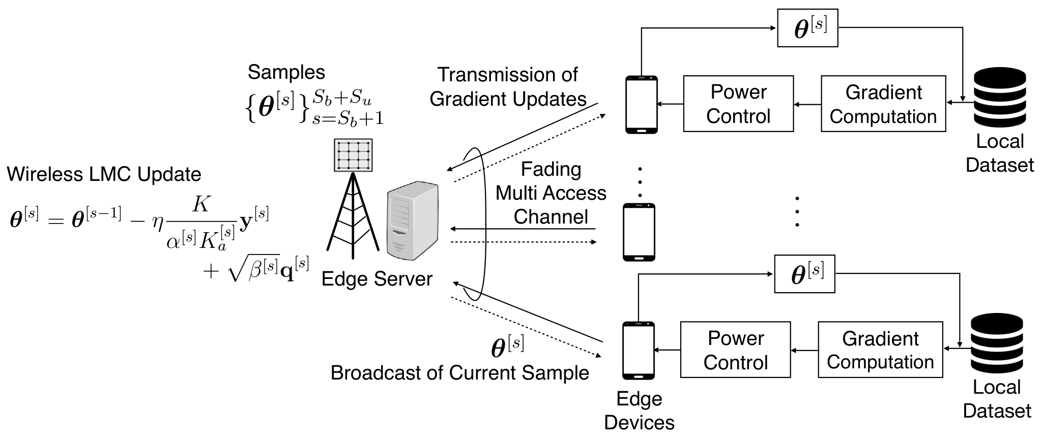
As shown in Fig. 1, we consider a wireless federated edge learning system comprising a single-antenna edge server and edge devices connected through it via a shared wireless channel. Each device , equipped with a single antenna, has its own local dataset encompassing data samples . For supervised learning applications, each data sample is in turn partitioned into a covariate vector and a label ; while, for unsupervised learning applications such as generative modeling, it consists of a single vector . The global data set is denoted as . The goal of the system is to carry out Bayesian learning via gradient-based Monte Carlo (MC) sampling. Accordingly, through communication with devices, the server wishes to obtain a number of random samples of the model parameter vector that are approximately distributed according to the global posterior distribution . Unlike [33], which studied one-shot protocols, the gradient-based MC methods studied in this paper are iterative, in a manner similar to standard federated learning protocols such as FedAvg.
II-A Langevin Monte Carlo
The machine learning model adopted by the system is defined by a likelihood function as well as by a prior distribution . Accordingly, the likelihood of the data at device is
| (1) |
where the likelihoods may be different across devices. The goal of Bayesian learning is to compute the global posterior
| (2) |
The global posterior can be expressed in terms of the local posteriors at each device , i.e.,
| (3) |
since we have the equality
| (4) |
In contrast, frequentist learning is concerned with the optimization of the global cost function
| (5) |
which is the log-loss evaluated from the unnormalized posterior (2). Minimizing the global cost function (5) yields the maximum a posterior (MAP) solution of frequentist learning. The global cost function (5) can be expressed in terms of the local cost functions
| (6) |
since we have the equality .
Directly computing the global posterior distribution (2) is generally of prohibitive complexity. To address this problem, Monte Carlo (MC) methods represent the global posterior distribution (2) in terms of samples approximately distributed from it. Specifically, Markov Chain MC (MCMC) techniques produce a sequence of samples with with the key property that as grows large, the marginal distribution of sample tends to the desired posterior distribution. As discussed in Sec. I, in this paper, we specifically adopt Langevin MC (LMC), a fundamental MCMC technique that has been widely studied as a means to strike a practical balance between complexity and efficiency (see, e.g., [12, 13]). LMC is a gradient-based MCMC sampling scheme building on the global cost function (5). As we elaborate on next, the LMC update is derived as an approximation of a continuous-time differential process that has the desired property of asymptotically producing samples drawn from the global posterior (2).
To start, we first introduce the continuous-time Langevin diffusion process (LDP) follows the stochastic differential equation
| (7) |
where represents Brownian motion. The Langevin diffusion process (7) has the invariant stable distribution , which corresponds to the desired global posterior (2) [35].
The integral of the stochastic differential equation (7) in the range of for integers and duration yields
| (8) |
where is a sequence of identical and independent (i.i.d.) random vectors following the Gaussian distribution . This is because we have the equality .
In the limit of a sufficiently small such that the following approximation holds
| (9) |
the discretization (8) results in Langevin MC (LMC), a gradient-based Markov chain MC (MCMC) sampling scheme that proceeds according to the iterative update rule
| (10) |
where we have and as step size. The error due to approximation (9) was studied in [32, 36], and it will be further discussed in Sec. IV-A.
In order to obtain samples approximately drawn from the global posterior distribution, LMC discards the samples produced in the first iterations (10), also known as burn-in period. The remaining samples with are retained and used for downstream applications such as ensemble prediction.
We consider LMC in this work due to its simplicity and scalability, as LMC updates amount to adding Gaussian noise to gradient descent updates. Other gradient-based MCMC methods, such as kinetic MC [14] and Hamilton MC [15], which modify higher-order updates may also be studied in a manner similar to this paper and are left for future research.
II-B Learning Protocol
The goal of the system under study is to implement LMC (10) in the described federated setting with devices, while satisfying formal differential privacy (DP) guarantees to be detailed in Sec. II-D. The protocols is organized in iterations with denoting the burn-in period, across which the server maintains sample iterates . The selection of burn-in period should avoid the regime in which the samples are too dependent on the Markov chain’s initialization. A formal test for this purpose is the Gelman-Rubin diagnostic, which is based by using multiple Markov chains. The diagnostic compares the estimated between-chains and within-chain variances for each model parameter, and chooses the burin-in period after which difference between theses variances are sufficiently small.
At each -th communication round, the edge server broadcasts the current sample to all edge devices via the downlink channel. We assume that downlink communication is ideal, so that each device receives the sample without distortion. This assumption is practically well justified when the edge server communicates through a base station with less stringent power constraint than the devices and the use of the whole downlink bandwidth for broadcasting. It is commonly made in many related papers, such as [5, 6, 7].
By using the received vector and the local dataset , each device computes the gradient of the local cost function (6) as
| (11) |
which is transmitted over the wireless shared channel to the edge server. The goal is to enable the edge server to approximate the update term in (10), namely
| (12) |
As we will see, channel noise can be repurposed to contribute to the additive random term in the LMC update (10). The steps in (11) and (10) are iterated across multiple communication rounds until a convergence condition is met. As a result, the server obtains a sequence of global model parameter vectors , with .
II-C Communication Model
The devices communicate via the uplink to the edge server on the shared wireless channel. The proposed approach leverages analog transmission in order to: (i) benefit from over-the-air computing as in many prior works [5, 17, 6]; and (ii) to repurpose channel noise for MC sampling and as a privacy mechanism. We assume a block flat-fading channel, where the channel coefficients remain constant within a communication block, and they vary in a potentially correlated way over successive blocks. Each block contains channel uses, allowing the uncoded transmission of a gradient vector via non-orthogonal multiple access (NOMA) as in [17, 6].
We assume symbol-level synchronization among the subset of devices that are scheduled in each block, enabling over-the-air computing. This can be achieved by using standard protocols such as the timing advance procedure in LTE and 5G NR [37]. In the -th communication round, the corresponding received signal is
| (13) |
where is the channel gain for device in round , is an uncoded function of the local gradient , and is channel noise i.i.d. according to distribution . The transmit power constraint of a device is given as
| (14) |
accounting for per-block power constraints.
II-D Performance Metrics
In this paper, we aim at designing a wireless federated learning protocol to implement Bayesian learning via Langevin MC under DP constraints. In this subsection, we formalize the performance criteria of interest and elaborate on the role of channel noise in achieving them.
II-D1 Approximation Error
Denoting as the distribution of the sample at the -th iteration, the quality of the sample is measured by the 2-Wasserstein distance between and the target global posterior in (2). This is defined as [32, 36]
| (15) |
where joint distribution is constrained to have marginals and . The Wasserstein distance is a standard measure of discrepancy between two distributions, and it is routinely used for the analysis of MC algorithms (see, e.g., [32, 36]). It has some useful properties with respect to other measures such as the Kullback-Leibler divergence and total variation distance. For instance, it is well defined and informative even when the two distributions have disjoint supports [38].
II-D2 Differential Privacy
We consider a “honest-but-curious” edge server that may attempt to infer information about local data sets from the received signals . We impose the standard -DP metric with some and , for each device . This amounts to the inequalities
| (16) |
for all , where is the number of communication rounds, and represents the distribution of the received signal (13) conditioned on the global data set . Condition (16) must hold for any two possible neighboring data sets and differing only by one sample, i.e., , and for all data sets of other devices.
II-D3 On the Role of Channel Noise
Without the additive random term in in (10), LMC coincides with standard gradient descent (GD) for frequentist learning, which was studied in [6] in a federated setting under the DP constraints (16). For convex models, the additive channel noise on the uplink channel (13) is harmful to the convergence rate of GD with no privacy constraints [6], although it can improve the generalization performance [4]. In [6, 28, 9], it was shown that channel noise can be repurposed to ensure the DP constraints (16) for values of that depend on the SNR level.
In this paper, we observe that, in Bayesian learning via MC, by (10), noise can potentially contribute not only to privacy but also to MC sampling, without necessarily compromising the learning performance. This idea was first introduced in [33] for one-shot MC sampling methods, and is studied here for the first time for iterative schemes. Specifically, we investigate the joint role of channel noise as a contributor to MC sampling and as a privacy-inducing mechanism. This interplay between MC sampling and DP was analyzed under ideal communication for centralized learning in [30], and the impact of channel noise in distributed settings is studied here for the first time.
II-E Assumptions on the Log-Likelihood
Finally, we list several standard assumptions we make on the global cost function in (5) and on its gradient.
Assumption 1 (Smoothness).
The global cost function is smooth with constant , that is, it is continuously differentiable and the gradient is Lipschitz continuous with constant , i.e.,
| (17) |
Assumption 2 (Strong Convexity).
The global cost function is strongly convex, i.e., the following inequality holds for some constant
| (18) |
Assumption 3 (Bounded Local Gradient).
The local gradient is bounded as
| (20) |
and some constant .
III Wireless Federated Langevin Monte Carlo (WFLMC)
In this section, we introduce wireless federated LMC (WFLMC). Specifically, we first present signal design and scheduling protocol, and then detail the rationale behind the proposed approach. The following sections will focus on the analysis of WFLMC.
III-A Signal Design and Scheduling Protocol
In each communication block, all devices transmit their local gradients simultaneously by using uncoded transmission of the form
| (21) |
for some power control parameter . Specifically, we implement truncated channel inversion as in [5, 7, 29], whereby the power control parameter is selected as
| (22) |
where gain parameter and threshold are parameters to be optimized. Accordingly, a device transmits only if its channel is large enough, i.e., . We note that this channel-aware scheduling aims to avoid deep fading channels. Other alternative scheduling policies may achieve better performance by considering also the importance of local data set, such as [41, 42]. We denote as the number of transmitting devices at round , and the corresponding set of transmitting devices.
To estimate the LMC update term (12) in (10), the received signal (13) is scaled and a Gaussian random vector is added. Specifically, wireless federated LMC (WFLMC) update is proposed as
| (23) |
where the added noise is independent of all other variables. The variance of the noise term is chosen as a function of the learning rate , channel noise , number of active users , and gain as
| (24) |
III-B Understanding WFLMC
To see the rationale behind the design (23)–(24), let us plug (13) and (21)–(22) into (23) to rewrite the WLMC update as
| (25) | ||||
| (26) |
where and are the i.i.d. sequences for , and we define
| (27) |
By (25), the power scaling (22) ensures that the gradients of the active devices sum at the receiver, and the scaling by in (23) of the received signal compensates for the resulting multiplier of the sum-gradient. The term is an empirical estimate of the gradient in (10) which is exact if .
Based on the discussion so far, in order for (25) to be an estimate of the LMC update (10), we should ideally ensure that the variance of the effective noise term be equal to . However, the power of this term, namely,
| (28) |
can only be partially controlled through power gain and added noise variance . In particular, we can always choose the added noise variance such that the variance is no smaller than . This condition is ensured by (24). In particular with (24), the effective noise in (25) can be decomposed into two parts as indicated in (26):
1) LMC noise: The term with serves the role of LMC noise with variance ;
2) Gradient estimation noise: The remaining noise, denoted as with , acts as a perturbation on the gradient estimate with variance in (27). Note that the variance of estimate noise is non-zero if the channel noise power is large.
IV Convergence and Privacy Analysis of WFLMC
In this section, we focus on the performance analysis of WFLMC in terms of (i) convergence through the 2-Wasserstein distance as defined in (15); and (ii) privacy under the DP criterion (16). In this section, we assume that the sequence of power gain and scheduling threshold parameters is fixed, and the results are given for an arbitrary sequence of channels.
IV-A Convergence Analysis
We now study the distribution of the sample produced by WFLMC via the updates (23). We recall that the goal of LMC is to produce samples distributed according to the global posterior . As discussed in Sec. II-D, we measure the approximation error via 2-Wasserstein distance (15).
There are three main contributions to the discrepancy between the distribution of and the target posterior :
- 1.
the initial discrepancy, which is measured by the 2-Wasserstein distance between the initial distribution and the posterior ;
- 2.
the gradient error in (26), namely
(29) which is caused by the excess noise and by the fact that only a subset of devices is active;
- 3.
and the discretization error due to the approximation (9), which is given as
(30)
We now bound the last two terms separately, and then use these results to bound square of the desired 2-Wasserstein distance in (15).
Lemma 1 (Upper Bound on the Gradient Error).
Proof: See Appendix -A.
The error bound (31) is comprised of two parts. The first term is the estimation error due to scheduling, which is zero if all the devices transmit in communication rounds, i.e., if . The second term is the variance of the excess noise in (27).
The discretization error is constant for for all communication round , and can be bounded by following [32, Lemma 3] as detailed in the next lemma.
Lemma 2 (Upper Bound on the Discretization Error).
Proof: The proof is detailed in Appendix -B.
Lemma 2 shows that the discretization error grows with model dimension , with the learning rate , and with the smoothness constant of the global cost function . Note that a larger implies a less smooth function .
Proposition 1 (Bound for 2-Wasserstein Distance).
Proof: The proof follows from the upper bound (see, e.g., [32])
| (36) |
where is obtained from the LDP (7), while is the sample produced by the LMC (10) with the LMC noise . Accordingly, the expectation is taken with respect to the Brownian motion in (7) and over the initial . Since, assuming the stationary of the LDP (7), the marginal of the LDP output is the target distribution for all , the bound (36) follows from the definition (15) by upper bounding the infimum with the described choice of the joint distribution of and .
Using (26) and (8), the right hand side of (36) can be computed as
| (37) |
The rest of the proof involves applying the geometric inequality for any , and using Lemma 1 and Lemma 2 as detailed in Appendix -C.
Proposition 1 indicates that the 2-Wasserstein distance depends on the initial discrepancy , whose contribution decreases exponentially with ; as well as the sum of contributions across the iteration index , with each -th error term weighted down by a factor decreasing exponentially with , i.e., as one moves towards earlier iterations. This shows that the disturbances at later communication rounds are more harmful to the approximation accuracy. Furthermore, the contribution of each iteration is given by the sum of the gradient error bounded in Lemma 1, and the discretization error bounded in Lemma 2.
Another interesting aspect highlighted by the bound (1) concerns the optimal choice of the learning rate . The upper bound (1) increases with in (33), and the minimum value of is attained when . However, a large learning rate causes the gradient error bound (31) and the discretization error bound (32) to increase by Lemma 1 and Lemma 2. Thus, the optimal learning rate is in the range of .
IV-B Differential Privacy Analysis
The WFLMC scheme implicitly implements a Gaussian DP mechanism [8, 30], since the channel noise in (25) is added to the disclosed function . Note that the noise in (25) is added by the edge server, and hence it does not contribute to privacy. Furthermore, while only part of the channel noise is useful for LMC (see (26)), the entire variance contributes to DP.
For the Gaussian mechanism, the privacy level depends on the sensitivity of the disclosed information and on the variance of the added noise [8, 6]. In a manner consistent to the definition (16) of DP, the sensitivity quantifies the maximum change of the disclosed function by replacing a single data point. The sensitivity for device is accordingly defined as
| (38) |
where and are computed by using data sets and respectively, and we have . By the triangular inequality and Assumption 3, we plug in the definition of (22) and have the bound
| (39) |
Following [6, Lemma 1], one can interpret the ratio as the privacy loss in each communication rounds. This is formalized in the following proposition.
Proposition 2 (DP Guarantees).
For any given sequence of parameters and channels , after communication rounds, WFLMC guarantees -DP if the following condition is satisfied
| (40) |
where is the inverse function of , and is the indicator function.
Proof: The result follows from [6, Lemma 1], although reference [6] did not account for the threshold-based scheduling in (22). The extension is direct by redefining the effective channel gain as .
In accordance to the discussion above, the left-hand side of (40) quantifies the overall privacy loss across rounds. Importantly, as anticipated, by (40) the channel noise power contributes in full to the DP performance. In contrast, by (26), only a portion of the channel noise contributes, in general, to the LMC update.
V Optimal Power Allocation and Scheduling
In this section, we leverage Proposition 1 and Proposition 2 to address the problem of minimizing the convergence error under the -DP constraint (40) and the power constraints (14) over power gain parameters and thresholds in (22). We recall that WFLMC carries out communication rounds for the burn-in period, which are followed by additional rounds to obtain the samples for use in downstream applications. The learning objective is to maximize the quality of the last samples under the mentioned privacy and power constraints, which apply for the total of communication rounds.
Throughout this section, we assume that the sequence of channels is known in advance in order to enable optimization. This assumption can be relaxed at the cost of additional communication overhead. Extensions to an online approach can be directly obtained by iterative one-step-ahead optimization based on predicted values for the future parameters as detailed in [6]. The optimization is conducted at the edge server. To control AirComp transmission, the edge server broadcasts the optimized at each communication round, which consumes a negligible amount of communication resources as compared with model broadcasting.
The joint power allocation and scheduling problem of interest is formulated as the min-max optimization
| (41a) | ||||
| (41b) | ||||
| (41c) | ||||
The maximization in (41a) aims at ensuring that the worst-case 2-Wasserstein distance is minimized across all samples after the burn-in period, under the DP constraint (41b) and the power constraint (41c). With its focus on the distribution of model parameters, problem (41) is notably distinct from the optimization problem for frequentist learning in [6], which only considers the quality of a single vector of model parameters in terms of training loss.
The problem (41) is non-convex since the objective function is non-differentiable in the thresholds . In fact, by (22), the threshold affects the objective function through the number of active users. To make progress, we fix the scalar thresholds and optimize over the power gain parameter .
V-A Zero Additive Noise is Optimal
We start by simplifying problem (41) through the following observation.
Lemma 3 (Zero Additive Noise).
Without compromising optimality, the variance of additive noise in (23) can be set as , which is equivalent to imposing the following constraint on the power gain parameters
| (42) |
Proof: Assume by contradiction that we had at an optimal solution. By (24), this would imply that the optimal satisfies the inequality . But one can always choose the smaller value , which achieves the same value of the objective function, while reducing the left-hand sides of the privacy and power constraints (41b)-(41c). This yields a contradiction, completing the proof.
The inequality (42) distinguishes two distinct regimes of operation of the system. If the equality (42) is active, the gradient estimation noise power in (27) is zero, and hence the channel noise contributes in full to the LMC updates. In contrast, when the inequality is strict, only a fraction of the channel noise is useful for LMC, and the rest contributes to the gradient estimation noise power .
V-B Optimization of Power Gain Parameters: Single-Sample and Constant Channels
We now tackle the optimization (41) over power gain parameters for the special case , and with constant channels and scheduling thresholds
| (43) | ||||
| (44) |
The solution in this special case will turn out to be especially insightful, and the more general problem will be studied in the next subsection. Under theses simplifying assumptions, and using Lemma 3, the min-max optimization in (41) reduces to the problem
| (45a) | ||||
| (45b) | ||||
| (45c) | ||||
| (45d) | ||||
Theorem 1.
Under Assumptions 1-3, and assuming static channels and thresholds as in (43)–(44), the optimal solutions of problem (45) depends on power and learning rate according to the three regimes illustrated in Fig. 2, which are detailed as follows.
- 1.
LMC-limited Regime: If the condition
(46) holds, the optimal power gain parameter is given as
(47) - 2.
Power-limited Regime: If the condition
(48) holds, the optimal power gain parameter is given as
(49) - 3.
DP-limited Regime: Otherwise, we have optimal solution
(50) where the value of can be obtained by bisection to satisfy the condition for the active devices .
Proof: The problem is seen to be convex by changing variables and the solution approach involves applying Lagrange multiplier method and Karush-Kuhn-Tucker (KKT) conditions in a manner similar to [6, Theorem 1]. Details can be found in Appendix -D.
The three regimes highlighted in Fig. 2 correspond to settings where each of the corresponding constraints, i.e., (47), (49) or (50), are active. Accordingly, we have the following observations:
In the LMC-limited regime, the channel noise contributes in full to LMC update, and hence the presence of channel noise and DP does not affect the performance of LMC. In contrast, in the other two regimes, the additional gradient noise causes a loss as compared to a noiseless implementation of LMC.
In the DP-limited regime, the privacy constraint affects the performance of WFLMC, while in the other regimes, privacy is obtained “for free”, i.e., as a direct consequence of the presence of channel noise. To optimize the learning performance, the power control parameter should be adaptive across the iterations.
V-C Optimization of Power Gain Parameters: General Case
In this subsection, we consider the general optimization problem (41) with any and under time-varying channels. To this end, we include LMC noise requirement leveraging Lemma 3, and start by rewriting the min-max optimization (41) in the epigraph form
| (51a) | ||||
| (51b) | ||||
| (51c) | ||||
| (51d) | ||||
| (51e) | ||||
Having made the change of variables , problem (51) can be easily seen to be convex. Therefore, it can be solved using standard numerical tools.
V-D Optimization of Truncated Thresholds
In this subsection, we turn to the problem of optimizing (41a) over the thresholds . As mentioned, this problem is characterized by a non-differentiable objective function, and it should be addressed jointly with the optimization of the power gain parameters . To make progress, we propose a sub-optimal approach that decouples the two problems by setting the value of to ensure equality in the constraint (41c) as
| (52) |
Note that the choice in (52) is only made for the purpose of optimizing the thresholds. After the thresholds are optimized as explained next, the power gain parameters are selected by following the previous subsections.
Using (52), the min-max problem (41a) over can be expressed as the sum of gradient error over communication rounds, for
| (53) |
where we have dropped the constraints since they are assumed to be dealt with by the subsequent optimization over . The minimization (53) can be addressed as parallel optimizations, and it is equivalent to focus on as
| (54) |
where the second term is obtained by the definition of in (27). The first term is estimation error depends on the bound of the norm of the local gradient as per Assumption 3. We note that this result can be directly extended to device-dependent bounds for each device . With this extension, the threshold in the scheduling rule (22) would depend on the properties of the local data set via constants .
The threshold affects the objective function (54) through the number of active users. Decreasing aggravates the estimation error (first term) due to partial scheduling, while providing a chance to alleviate the excess noise (second term) by silencing the devices with the worst channels. The objective function (54) can take at most different values that are attained by setting as one of the channel gains . Therefore, we can limit the search to these values without loss of optimality. It follows that the optimal solution for each threshold can be obtained by exhaustive search over the values by minimizing (54).
VI Numerical Results
In this section, we investigate the effectiveness of the proposed scheme, WFLMC, as a mechanism to implement LMC on wireless channels using numerical experiments. We emphasize that our goal is not that of comparing the performance of Bayesian and frequentist techniques. This is a subject that has been extensively explored in the literature (see Sec. I), and we consider it to be beyond the scope of this contribution. Rather, our focus is on evaluating the effectiveness of the specific proposed implementation mechanism of LMC as compared to more conventional solutions. To this end, we consider the following benchmark schemes.
- 1)
WFMLC with equal power allocation: This reference scheme follows the approach in [28] of dividing up the DP constraint equally across all communication rounds. By Lemma 2, this corresponds to imposing the constraint
(55) for each communication round. Condition (55), along with the power constraint (41c) and LMC noise requirement (42) yield the power scaling gains
(56) - 2)
WFLMC without DP constraint: In this scheme, the power gain parameter is set as
(57) which corresponds to the optimal solution without the DP constraint.
We also consider for reference a scenario characterized by ideal communication without fading (i.e., ), and channel noise (i.e., ). To guarantee privacy and implement LMC update, noise is added at each devices before transmission as
| (58) |
and . The variance depends on the DP constraint. Specifically, following the analysis in WFLMC, we can define the following two additional benchmark schemes.
- 3)
- 4)
As for the learning model, we consider a Gaussian linear regression with likelihood
| (59) |
and the prior is assumed to follow Gaussian distribution . Therefore, the posterior is the Gaussian , where is the data matrix and is the label vector. The strong convexity parameter and smoothness parameter are computed as the smallest and largest eigenvalues of the data Gramian matrix . We will also consider experiments with the MNIST data set at the end of this section.
We consider a synthetic data set with following the model (59) with covariates drawn i.i.d. from Gaussian distribution where , and ground-truth model parameter . The Wasserstein distance between two Gaussian distribution and is computed as [44]
| (60) |
Unless stated otherwise, we consider homogeneous local data distributions by dividing the data set equally among the devices. In this regard, we observe that Bayesian learning is generally not impacted by “non-i.i.d.” data distributions in the sense that global posterior is well defined irrespective of data homogeneity or heterogeneity at the devices. That said, in the presence of privacy constraint, the need for clipping causes centralized and federated implementations of LMC to be different, and the performance loss of federated against centralized LMC becomes more pronounced for a smaller clipping threshold in the presence of heterogeneous distribution. Here we set the clipping threshold to , and leave an investigation of the interplay between data heterogeneity and clipping to future work. Furthermore, the initial sample is drawn from prior with discrepancy .
VI-A Single-Sample Case
We now focus on single-sample case () by applying the optimal power allocation detailed in Theorem 1 while scheduling all devices (). As in Theorem 1, the channels are constant and set to for all devices ; the number of communication burn-in periods is set to ; DP parameters are given as and .
Impact of the SNR: In Fig. 3, we plot the bound (1) on the 2-Wasserstein distance versus SNR, defined as , by varying transmitted power . The learning rate is set as and in order to illustrate the different regimes defined in Fig. 2. In Fig. 3(a), under the larger learning rate, the performance is limited by the power constraint until dB, after which it becomes limited by DP. In the DP-limited regime, optimized power allocation attains better performance than static power allocation. For dB, the performance under optimized power allocation becomes equivalent to that of the system with ideal noiseless communication with the DP, showing that all channel noise is repurposed for DP mechanism while only partial is for MC sampling. That is, imposing the DP constraint causes some performance loss due to the need of scaling down the transmission power to decrease the effective SNR. In line with the results in Fig. 2, Fig. 3(b) shows the transition from power-limited regime to LMC-limited regime for the smaller learning rate. In the LMC-limited regime, all the schemes have same performance since the channel noise variance is only determined by the LMC constraint.
Impact of the learning rate: We now further elaborate on the impact of the learning rate in Fig. 4 by setting dB and dB. First, with , by Fig. 2, we are in the LMC-limited regime where all the schemes have same performance. When , the performance of optimized power allocation is shown to be power-limited for dB in Fig. 4(a), as it is identical to that without the DP constraint. In contrast, when dB, as seen in Fig. 4(b), the performance of optimized power allocation is limited by DP for . As for the static power allocation, the performance is always limited by DP for , and increasing the SNR is not helpful in reducing the approximation error.
Impact of the privacy level: Fig. 6 plots the bound (1) on the 2-Wasserstein distance as a function of the privacy level . The performance of WFLMC is limited by DP until , after which it becomes limited by the transmitted power and the DP constraint does not cause a performance loss. In the DP-limited regime, the proposed optimized power allocation outperforms static power allocation. Furthermore, under a stricter DP requirement, i.e., with , the performance of optimized power allocation is equivalent to that under ideal communication, and the existence of channel noise does not impair performance.
VI-B Multi-Sample Case
We obtain the power control strategy in the multi-sample case by solving the convex problem (51) under the suboptimal scheduling policy in (54). The optimized parameters are then used to implement WLMC. To evaluate the 2-Wasserstein distance, we numerically estimate the mean and covariance matrices of the samples over 100 experiments, and compare with the true posterior via (60). The results present as the worst performance after the burn-in period, as given in the objective (41a). Unless stated otherwise, the channels are randomly generated following for all ; the number of communication round is set to ; DP parameters are set to and .
Impact of the SNR: We first study the impact of the with number of samples . The Wasserstein distances of all the wirelesses LMC schemes are seen to decrease with the SNR until approaching the DP-limited regime for optimized power allocation, and the LMC-limited regime for the scheme without DP constraint. The results emphasize the importance of optimizing power allocation in high SNR regime where the static power allocation is seen to have a significant performance degradation in DP-limited regime. Furthermore, they validate the insights obtained for the analysis under the simplified assumptions considered in Theorem 1.
Impact of the Burn-in Period: In Fig. 8, we investigate the impact of the number of communication periods, , allocated for the burn-in period where we fix as the total number of communication rounds. In this experiment, the SNR is set to dB. Fig. 8 shows that increasing the communication rounds in the burn-in period helps improve the quality of the samples produced after the burn-in period, as the Wasserstein distances of all the schemes are seen to decrease with the burn-in period. We also note that the enhanced sample quality costs at the cost of sample quantity. The performance of LMC is limited by the bias in discretization error that is determined by the learning rate and can not be diminished by increasing the duration of the burn-in period. Overall, the results emphasize that sample quality can be enhanced by optimizing the power allocation strategy.
VI-C MNIST Data Set
We now consider the problem of multinomial logistic regression on the MNIST data set, which is comprised of classes representing handwritten digits. We use data points, and data points for each class are randomly selected from the MINST training set. The original data, with dimension , is pre-processed by projecting the input images into a subspace of lower dimension via principal component analysis (PCA). This is motivated by the fact that the MNIST images are known to be approximately supported on a manifold with intrinsic dimension lower than 30 [45].
For the learning model, the likelihood is considered as
| (60) |
where we have . The prior of the model parameters is a produced Gaussian distribution for . To set the parameters and , we leverage the inequality for the Hessian matrix , where is a matrix with all elements , and represents Kronecker product. Specifically, we compute the minimum and maximum eigenvalues of the lower bound and upper bound respectively to set and . The channels are randomly generated following the distribution for all ; the number of communication round is set to ; the number of communication burn-in periods is set to ; the clipping threshold in (20) is set to ; and DP parameters are set to and . The results are averaged over 50 experiments.
For tractability, the optimization problem aims at minimizing the averaged Wasserstein distances across the samples after the burn-in period. The problem is convex and can be solved by the method in Sec V-B. We use the test set of MNIST to evaluate the expected calibration error [10]. Furthermore, we implemented scalable Bayesian federated learning (SBFL) in [19] as another benchmark. We recall that SBFL is a frequentist learning protocol that aggregates the local gradients at the server via a point estimate that incorporates prior knowledge on the gradients. Under the assumption of orthogonal multiple access in [19], the iteration time is set as for a fair comparison.
Fig. 8 plots the expected calibration error versus SNR with the number of samples . First, the figure verifies the advantage of Bayesian learning, as all WFLMC schemes are seen to significantly outperform SBFL. Furthermore, by increasing the number of communication rounds, optimized power allocation can outperform the equal power allocation scheme.
VII Conclusions
In this paper, we have proposed a novel Bayesian federated learning (FL) protocol that implements Langevin Monte Carlo (LMC) via uncoded wireless transmission from devices to edge server. The learning protocol is enabled by over-the-air computing, which is akin to previous works on wireless (frequentist) FL [5, 6], as well as by the novel idea of repurposing channel noise for MC sampling in Bayesian FL. The goal is to obtain samples at the edge server that are approximately drawn according to the global posterior distribution. The key idea of this work is to leverage the channel noise for both MC sampling and privacy preservation. Under simplified assumptions, the analysis has revealed that system operating different regimes limited by LMC, DP or power constraints, depending on the values of learning rate, privacy parameters, and transmitted power. As for the general case, the problem of optimizing power allocation was proved to be convex. Simulation results have validated the analysis, yielding insights into conditions under which channel noise is not harmful to the system performance.
As an extension of the current work, it is interesting to optimize the learning rate schedule, which may not only benefit learning performance but also enhance privacy. Another direction is to study digital implementations of wireless federated LMC as in [7]. The current work can also be further generalized to multi-hop device-to-device (D2D) network topologies. The analysis could also be extended to the scenario of non-ideal downlink communication as in [46, 47].
-A Proof of Lemma 1
-B Proof of Lemma 2
The vector is the continuous-time Langevin diffusion process in (7) and its distribution is assumed to be invariant, so that we have for all . The proof follows from [32, Lemma 3] with the caveat that we bound of in lieu of . This is done as:
| (61) |
where and are consequences of Cauchy-Schwarz inequality and of the interchanging the order of expectation and integral; is obtained by Assumption 1 and (8); is derived using [32, Lemma 2].
-C Proof of Proposition 1
For any , the error (IV-A) is bounded as
| (62) |
where the value of controls the convergence rate as detailed later. Furthermore, the first term is bounded by
| (63) |
where if ; and if . The proof starts with (II-E) through [32, Lemma 1]. Specifically, plugging Lemmas 1 and 2 and (63) into (-C), and setting yield
| (64) |
The desired result in Proposition 1 is obtained by using the inequality , applying (-C) recursively, and the initial point is set to satisfy .
-D Proof of Theorem 1
Substituting with , and , the optimization problem (45) is equivalent to the following convex program
| (65a) | ||||
| (65b) | ||||
| (65c) | ||||
| (65d) | ||||
To solve this problem, the partial Lagrange function is defined as
| (66) |
where , , and are the Lagrange multipliers associated respectively with the DP constraint, non-negative parameter constraints, joint transmit power and non-negative noise variance constraints. Then, applying the KKT conditions leads to the following necessary and sufficient conditions for optimality
| (67a) | ||||
| (67b) | ||||
| (67c) | ||||
| (67d) | ||||
| (67e) | ||||
| (67f) | ||||
| (67g) | ||||
Combing (67a) and (67d) we have
| (68) |
On the other hand, (67c) indicates, that if , then we have
| (69) |
Furthermore, according to (67b), if condition
| (70) |
holds, we have , and thus for all with the optimal value of given in (69). Otherwise we have the following equality
| (71) |
and the optimal solution is
| (72) |
The solution of is obtained by solving (71). Reverting to the original variables via and separating the solution (69) into and yield desired results in the theorem.
References
- [1] J. Park, S. Samarakoon, M. Bennis, and M. Debbah, “Wireless network intelligence at the edge,” Proc. IEEE, vol. 107, no. 11, pp. 2204–2239, 2019.
- [2] G. Zhu, D. Liu, Y. Du, C. You, J. Zhang, and K. Huang, “Toward an intelligent edge: wireless communication meets machine learning,” IEEE Commun. Mag., vol. 58, pp. 19–25, Jan. 2020.
- [3] T. Sery, N. Shlezinger, K. Cohen, and Y. C. Eldar, “Over-the-air federated learning from heterogeneous data,” IEEE Trans. Signal Process., vol. 69, pp. 3796–3811, June 2021.
- [4] H. H. Yang, Z. Chen, T. Q. Quek, and H. V. Poor, “Revisiting analog over-the-air machine learning: The blessing and curse of interference,” [Online]. Available: https://arxiv.org/pdf/2107.11733.pdf, 2021.
- [5] G. Zhu, Y. Wang, and K. Huang, “Broadband analog aggregation for low-latency federated edge learning,” IEEE Trans. Wireless Commun., vol. 19, pp. 491–506, Oct. 2019.
- [6] D. Liu and O. Simeone, “Privacy for free: Wireless federated learning via uncoded transmission with adaptive power control,” IEEE J. Sel. Areas Commun., vol. 39, pp. 170–185, Nov. 2020.
- [7] G. Zhu, Y. Du, D. Gündüz, and K. Huang, “One-bit over-the-air aggregation for communication-efficient federated edge learning: Design and convergence analysis,” IEEE Trans. Wireless Commun., vol. 20, pp. 2120–2135, March 2021.
- [8] C. Dwork, A. Roth, et al., “The algorithmic foundations of differential privacy,” Foundations and Trends® in Theoretical Computer Science, vol. 9, no. 3–4, pp. 211–407, 2014.
- [9] Y. Koda, K. Yamamoto, T. Nishio, and M. Morikura, “Differentially private aircomp federated learning with power adaptation harnessing receiver noise,” in Proc. IEEE Glob. Commun. Conf. (GLOBECOM), (Virtual), Dec. 2020.
- [10] C. Guo, G. Pleiss, Y. Sun, and K. Q. Weinberger, “On calibration of modern neural networks,” in Proc. Intl. Conf. Mach. Learning (ICML), (Sydney, Australia), pp. 1321–1330, Aug. 2017.
- [11] B. Lakshminarayanan, A. Pritzel, and C. Blundell, “Simple and scalable predictive uncertainty estimation using deep ensembles,” [Online]. Available: https://arxiv.org/pdf/1612.01474.pdf, 2016.
- [12] E. Angelino, M. J. Johnson, and R. P. Adams, “Patterns of scalable bayesian inference,” [Online]. Available: https://arxiv.org/pdf/1602.05221.pdf, 2016.
- [13] Y.-A. Ma, T. Chen, and E. Fox, “A complete recipe for stochastic gradient MCMC,” in Proc. Adv. Neural Info. Proc. Syst. (NIPS), vol. 28, (Montreal, Canada), Dec. 2015.
- [14] A. S. Dalalyan and L. Riou-Durand, “On sampling from a log-concave density using kinetic langevin diffusions,” Bernoulli, vol. 26, no. 3, pp. 1956–1988, 2020.
- [15] D. Zou and Q. Gu, “On the convergence of hamiltonian monte carlo with stochastic gradients,” in Proc. Conf. Mach. Learning (ICML), (Virtual), pp. 13012–13022, July 2021.
- [16] D. Alistarh, D. Grubic, J. Li, R. Tomioka, and M. Vojnovic, “QSGD: Communication-efficient SGD via gradient quantization and encoding,” in Proc. Adv. Neural Info. Proc. Syst. (NIPS), (Long Beach, USA), Dec. 2017.
- [17] T. Sery and K. Cohen, “On analog gradient descent learning over multiple access fading channels,” IEEE Trans. Signal Process., vol. 68, pp. 2897–2911, 2020.
- [18] D. Fan, X. Yuan, and Y.-J. A. Zhang, “Temporal-structure-assisted gradient aggregation for over-the-air federated edge learning,” [Online]. Available: https://arxiv.org/pdf/2103.02270.pdf, 2021.
- [19] S. Lee, C. Park, S.-N. Hong, Y. C. Eldar, and N. Lee, “Bayesian federated learning over wireless networks,” [Online]. Available: https://arxiv.org/pdf/2012.15486.pdf, 2020.
- [20] H.-Y. Chen and W.-L. Chao, “Fedbe: Making bayesian model ensemble applicable to federated learning,” in Proc. Intl. Conf. Learning Representations (ICLR), (Virtual), May 2021.
- [21] Z. Zhu, J. Hong, and J. Zhou, “Data-free knowledge distillation for heterogeneous federated learning,” [Online]. Available: https://arxiv.org/pdf/2105.10056.pdf, 2021.
- [22] L. Corinzia and J. M. Buhmann, “Variational federated multi-task learning,” [Online]. Available: https://arxiv.org/pdf/1906.06268.pdf, 2019.
- [23] R. Kassab and O. Simeone, “Federated generalized bayesian learning via distributed stein variational gradient descent,” [Online]. Available: https://arxiv.org/pdf/2009.06419.pdf, 2020.
- [24] K. el Mekkaoui, D. Mesquita, P. Blomstedt, and S. Kaski, “Federated stochastic gradient langevin dynamics,” in Proc. 37th Conf. Uncertain. Artif. Intell. (UAI), (Virtual), July 2021.
- [25] M. Vono, V. Plassier, A. Durmus, A. Dieuleveut, and E. Moulines, “QLSD: Quantised Langevin stochastic dynamics for Bayesian federated learning,” [Online]. Available: https://arxiv.org/pdf/2106.00797.pdf, 2021.
- [26] V. Gandikota, R. K. Maity, and A. Mazumdar, “vqSGD: Vector quantized stochastic gradient descent,” [Online]. Available: https://arxiv.org/pdf/1911.07971.pdf, 2019.
- [27] N. Agarwal, A. T. Suresh, F. X. X. Yu, S. Kumar, and B. McMahan, “cpSGD: Communication-efficient and differentially-private distributed SGD,” in Proc. Adv. Neural Info. Proc. Syst. (NIPS), (Montreal, Canada), Dec. 2018.
- [28] M. Seif, R. Tandon, and M. Li, “Wireless federated learning with local differential privacy,” in Proc. IEEE Intl. Symp. Info. Theory (ISIT), (Los Angeles, USA), June 2020.
- [29] Z. Zhang, G. Zhu, R. Wang, V. K. Lau, and K. Huang, “Turning channel noise into an accelerator for over-the-air principal component analysis,” [Online]. Available: https://arxiv.org/pdf/2104.10095.pdf, 2021.
- [30] Y.-X. Wang, S. Fienberg, and A. Smola, “Privacy for free: Posterior sampling and stochastic gradient Monte Carlo,” in Proc. Conf. Mach. Learning (ICML), (Lille, France), July 2015.
- [31] B. Li, C. Chen, H. Liu, and L. Carin, “On connecting stochastic gradient MCMC and differential privacy,” in Proc. Intl. Conf. Artif. Intell. Stat. (AISTATS), (Naha, Japan), April 2019.
- [32] A. Dalalyan, “Further and stronger analogy between sampling and optimization: Langevin monte carlo and gradient descent,” in Proc. Conf. Learning Theory (COLT), (Amsterdam, Netherlands), July 2017.
- [33] D. Liu and O. Simeone, “Channel-driven Monte Carlo sampling for Bayesian distributed learning in wireless data centers,” [Online]. Available: https://arxiv.org/pdf/2103.01351.pdf, 2021.
- [34] M. Rabinovich, E. Angelino, and M. I. Jordan, “Variational consensus Monte Carlo,” in Proc. Adv. Neural Info. Proc. Syst. (NIPS), (Montreal, Canada), Dec. 2015.
- [35] R. Bhattacharya et al., “Criteria for recurrence and existence of invariant measures for multidimensional diffusions,” The Annals of Probability, vol. 6, no. 4, pp. 541–553, 1978.
- [36] N. Chatterji, N. Flammarion, Y. Ma, P. Bartlett, and M. Jordan, “On the theory of variance reduction for stochastic gradient monte carlo,” in Proc. Intl. Conf. Mach. Learning (ICML), (Stockholm, Sweden), pp. 764–773, July 2018.
- [37] A. Mahmood, M. I. Ashraf, M. Gidlund, J. Torsner, and J. Sachs, “Time synchronization in 5G wireless edge: Requirements and solutions for critical-mtc,” IEEE Commun. Mag., vol. 57, pp. 45–51, Dec. 2019.
- [38] M. Arjovsky, S. Chintala, and L. Bottou, “Wasserstein generative adversarial networks,” in Proc. Intl. Conf. Mach. Learning (ICML), (Sydney, Australia), pp. 214–223, Aug. 2017.
- [39] S. Bubeck, “Convex optimization: Algorithms and complexity,” Found. Trends Mach. Learn., vol. 8, pp. 231–357, Nov. 2015.
- [40] X. Chen, Z. S. Wu, and M. Hong, “Understanding gradient clipping in private SGD: A geometric perspective,” in Proc. Adv. Neural Info. Proc. Syst. (NIPS), (Virtual), Dec. 2020.
- [41] J. Ren, Y. He, D. Wen, G. Yu, K. Huang, and D. Guo, “Scheduling for cellular federated edge learning with importance and channel awareness,” IEEE Trans. Wireless Commun., vol. 19, no. 11, pp. 7690–7703, 2020.
- [42] D. Liu, G. Zhu, J. Zhang, and K. Huang, “Data-importance aware user scheduling for communication-efficient edge machine learning,” IEEE Transactions on Cognitive Communications and Networking, vol. 7, no. 1, pp. 265–278, 2020.
- [43] D. Liu and O. Simeone, “Wireless federated langevin monte carlo: Repurposing channel noise for bayesian sampling and privacy,” [Online]. Available: https://arxiv.org/pdf/2108.07644.pdf, 2021.
- [44] C. Sun, H. Yan, X. Qiu, and X. Huang, “Gaussian word embedding with a wasserstein distance loss,” [Online]. Available: https://arxiv.org/pdf/1808.07016.pdf, 2018.
- [45] M. Hein and J.-Y. Audibert, “Intrinsic dimensionality estimation of submanifolds in rd,” in Proc. Intl. Conf. Mach. Learning (ICML), (Bonn, Germany), Aug. 2005.
- [46] X. Wei and C. Shen, “Federated learning over noisy channels: Convergence analysis and design examples,” [Online]. Available: https://arxiv.org/pdf/2101.02198.pdf, 2021.
- [47] M. M. Amiri, D. Gündüz, S. R. Kulkarni, and H. V. Poor, “Convergence of federated learning over a noisy downlink,” IEEE Transactions on Wireless Communications, 2021.