Light Field Image Super-Resolution with Transformers
Abstract
Light field (LF) image super-resolution (SR) aims at reconstructing high-resolution LF images from their low-resolution counterparts. Although CNN-based methods have achieved remarkable performance in LF image SR, these methods cannot fully model the non-local properties of the 4D LF data. In this paper, we propose a simple but effective Transformer-based method for LF image SR. In our method, an angular Transformer is designed to incorporate complementary information among different views, and a spatial Transformer is developed to capture both local and long-range dependencies within each sub-aperture image. With the proposed angular and spatial Transformers, the beneficial information in an LF can be fully exploited and the SR performance is boosted. We validate the effectiveness of our angular and spatial Transformers through extensive ablation studies, and compare our method to recent state-of-the-art methods on five public LF datasets. Our method achieves superior SR performance with a small model size and low computational cost. Code is available at https://github.com/ZhengyuLiang24/LFT.
Index Terms:
Light field, image super-resolution, transformerI Introduction
Light field (LF) cameras record both intensity and directions of light rays, and enable many applications such as post-capture refocusing[1, 2], depth sensing [3, 4], saliency detection[5] and de-occlusion [6, 7]. Since high-resolution (HR) images are required in various applications, it is necessary to use the complementary information among different views (i.e., angular information) to achieve LF image super-resolution (SR).
In the past few years, convolutional neural networks (CNNs) have been the dominant architectures of LF image SR. Yoon et al. [8] proposed the first CNN-based method called LFCNN to improve the resolution of LF images. Then, some works[9, 10, 11, 12, 13] combined CNN-based method with the epipoloar geometry of LF images to improve the SR performance. Several works [14, 15, 16, 17] organized LF images into the sub-aperture and macro-pixel patterns to achieve LF image SR. Meng et al.[18] designed a high-dimensional dense residual network to learn the geometry information encoded in multiple adjacent views.
Although the SR performance has been continuously improved via delicate network designs, most existing CNN-based LF image SR methods have the following two limitations. First, these methods either use part of views to reduce the complexity of the 4D LF structure [8, 9, 10, 11], or integrate angular information without considering view position and image content [15, 16, 13]. The under-use of the rich angular information results in performance degradation especially on complex scenes (e.g., occlusions and non-Lambertain surfaces). Second, existing CNN-based methods extract spatial features by applying (cascaded) convolutions on SAIs. The local receptive field of convolutions hinders these methods to capture long-range spatial dependencies from input images. In summary, existing CNN-based LF image SR methods cannot fully exploit both angular and spatial information, and thus face a bottleneck for further performance improvement.
Recently, Transformers have been demonstrated effective in modeling positional and long-range correlations, and were applied to various computer vision tasks such as image classification [19], object detection [20, 21], semantic segmentation [22], depth estimation [23] and super-resolution[24, 25]. More research and details about Transformers can be referred to Section II. Inspired by the recent advances of Transformers, in this paper, we propose a Transformer-based network (i.e., LFT) to address the aforementioned limitations of CNN-based methods. Specifically, we design an angular Transformer to model the relationship among different views, and design a spatial Transformer to capture both local and non-local context information within each SAI. Compared to CNN-based methods, our LFT can discriminately incorporate the information from all angular views, and capture long-range spatial dependencies in each SAI.
The contributions of this paper can be summarized as: 1) We adapt Transformers to LF image processing and propose a simple but strong baseline for LF image SR. 2) We propose a novel paradigm (i.e., angular and spatial Transformers) to incorporate angular and spatial information in an LF. The effectiveness of our paradigm is validated through extensive ablation studies. 3) With a small model size and low computational cost, our LFT achieves superior SR performance than other state-of-the-art methods.

II Related Work
II-A LF Image SR
Since the CNNs are first introduced to the area of LF image SR [8], CNNs have been widely used and the performance of reconstruction has been continuously developed [9, 10, 11, 12, 13, 14, 15, 16, 17, 18]. Yuan et al. [9] applied EDSR [26] to super-resolve each sub-aperture image (SAI) independently, and developed an EPI-enhancement network to refine the super-resolved images. Yeung et al.[14] proposed LFSSR to alternately shuffle LF features between sub-aperture and macro-pixel patterns for convolution. Zhang et al. [11] proposed a multi-branch residual network to incorporate the multi-directional epipolar geometry prior for LF image SR. More recently, Zhang et al. [12] divided LF images into several image stacks according to multiple epipolar geometry, and fed them into different branches to effectively learn sub-pixel information. Since both view-wise angular information and image-wise spatial information contribute to the SR performance, state-of-the-art CNN-based methods [13, 15, 16, 17, 18] designed different network structures to leverage both angular and spatial information for LF image SR. In [15], the spatial and angular features can be separately extracted from LF images, and then repetitively interacted to progressively incorporate spatial and angular information. Jin et al. [13] proposed an all-to-one framework to super-resolve each view using all the remaining views, and designed a structure-aware loss to preserve the parallax structure of LF images. Meng et al. [18] designed a high-dimensional dense residual network (i.e., HDDRNet), and applied 4D convolutions to learn the geometry information encoded in multiple adjacent views.
II-B Vision Transformers
Different from the convolutions that process an image locally, vision Transformers regards an image as a sequence of tokens, and build the relationship between the pairs of all tokens by self-attention mechanism. Thanks to the capability of modeling long-range dependencies (i.e., the relationship of all tokens), Transformers have achieved competitive performance on many vision tasks, e.g., object detection [21], classification [20] and semantic segmentation [22]. Among them, Carion et al. [21] first applied Transformers to object detection to model the relations of objects and global image contexts, and directly generate the set of predictions in detection. Dosovitskiy et al. [19] designed a pure Transformer model (i.e., ViT) for classification tasks, and ViT achieves competitive results as compared to CNN-based methods. Zheng et al. [22] treated semantic segmentation as a sequence-to-sequence prediction task, and designed a pure Transformer encoder and a CNN-based decoder to model global context and pixel-level segmentation, respectively. In the area of low-level vision, Chen et al. [27] developed an image processing Transformer with multi-heads and multi-tails. Their method achieves state-of-the-art performance on image denoising, deraining, and SR. Wang et al.[24] proposed a hierarchical U-shaped Transformer to capture both local and non-local context information for image restoration. Cao et al. [25] proposed a Transformer-based network to exploit correlations among different frames for video SR.
III Method
We formulate an LF as a 4D tensor , where and represent angular dimensions, and represent spatial dimensions. Following [11, 14, 18, 13, 15], we achieve LF image SR using SAIs distributed in a square array (i.e., ==). As shown in Fig. 1(a), our network consists of three stages including initial feature extraction, Transformer-based feature incorporation, and up-sampling.
III-A Angular Transformer
The input LF images are first processed by cascaded 33 convolutions to generate initial features . The extracted features are then fed to the angular Transformer to model the angular dependencies. Our angular Transformer is designed to correlate highly relevant features in the angular dimension and can fully exploit the complementary information among all the input views.
Specifically, feature is first reshaped into a sequence of angular tokens , where represents the batch dimension, is the length of the sequence and denotes the embedding dimension of each angular token. Then, we perform angular positional encoding to model the positional correlation of different views [28], i.e.,
| (1) |
| (2) |
where represents the angular position and denotes the channel index in embedding dimension. It is worth mentioning that each dimension of the positional encoding vector is regarded as a sinusoid, and represents the wavelength of sinusoids to form a geometric progression from 2 to 2 for the angular positional encoding. Following [28], we set to 10000 in our experiments.
As shown in Fig. 1(b) and Fig. 1(d), the angular position codes are directly added to , and passed through a layer normalization (LN) to generate query and key , i.e., . Value is directly assigned as , i.e., . Afterwards, we apply the multi-head self-attention (MHSA) to learn the relationship among different angular tokens. Similar to other MHSA approaches [28, 27, 19], the embedding dimension of , and is split into groups, where is the number of heads. For each attention head, the calculation can be formulated as:
| (3) |
where denotes the index of head groups. , and are the linear projection matrices. In summary, the MHSA can be formulated as:
| (4) |
where is output projection matrix, denotes the concatenation operation.
As shown in Fig. 1(b), to further incorporate the correlations built by MHSA, the tokens are further fed to a feed forward network (FFN), which consists of a LN and a multi-layer perception (MLP) layer. In summary, the calculation process of our angular Transformer can be formulated as:
| (5) |
| (6) |
Finally, is reshaped into and fed to the subsequent spatial Transformer to incorporate spatial context information.
III-B Spatial Transformer
The goal of our spatial Transformer is to leverage both local context information and long-range spatial dependencies within each SAI. Specifically, the input feature is first unfolded in each 33 neighbor region [29], and then fed to an MLP to achieve local feature embedding. That is,
| (7) |
where denotes an arbitrary spatial coordinate on feature . The local assembled feature is then cropped into overlapping spatial tokens , where denotes the batch dimension, represents the length of the sequence, and represents the embedding dimension of the spatial tokens.
By performing feature unfolding and overlapped cropping, the local context information can be fully integrated into the generated spatial tokens, which enables our spatial Transformer to model both local and non-local dependencies. To further model the spatial position information, we perform 2D positional encoding on spatial tokens:
| (8) |
| (9) |
where denotes the spatial position, denotes the index in the embedding dimension and parameter is set as 10000. Then, , and can be calculated according to:
| (10) |
| (11) |
As shown in Fig. 1(c), similar to the proposed angular Transformer, we use the MHSA and FFN to build our spatial Transformer. That is,
| (12) |
| (13) |
Then, is reshaped into and fed to the next angular Transformer. After passing through all the angular and spatial Transformers, both angular and spatial information in an LF can be fully incorporated. Finally, we apply pixel shuffling [30] to achieve feature up-sampling, and obtain the super-resolved LF image .
IV Experiments
| Methods | ||||||||||
| EPFL | HCInew | HCIold | INRIA | STFgantry | EPFL | HCInew | HCIold | INRIA | STFgantry | |
| Bicubic | 29.74/0.941 | 31.89/0.939 | 37.69/0.979 | 31.33/0.959 | 31.06/0.954 | 25.14/0.833 | 27.61/0.853 | 32.42/0.931 | 26.82/0.886 | 25.93/0.847 |
| VDSR [31] | 32.50/0.960 | 34.37/0.956 | 40.61/0.987 | 34.43/0,974 | 35.54/0.979 | 27.25/0.878 | 29.31/0.883 | 34.81/0.952 | 29.19/0.921 | 28.51/0.901 |
| EDSR [26] | 33.09/0.963 | 34.83/0.959 | 41.01/0.988 | 34.97/0.977 | 36.29/0.982 | 27.84/0.886 | 29.60/0.887 | 35.18/0.954 | 29.66/0.926 | 28.70/0.908 |
| RCAN [32] | 33.16/0.964 | 34.98/0.960 | 41.05/0.988 | 35.01/0.977 | 36.33/0.983 | 27.88/0.886 | 29.63/0.888 | 35.20/0.954 | 29.76/0.927 | 28.90/0.911 |
| resLF[11] | 33.62/0.971 | 36.69/0.974 | 43.42/0.993 | 35.39/0.981 | 38.36/0.990 | 28.27/0.904 | 30.73/0.911 | 36.71/0.968 | 30.34/0.941 | 30.19/0.937 |
| LFSSR [14] | 33.68/0.974 | 36.81/0.975 | 43.81/0.994 | 35.28/0.983 | 37.95/0.990 | 28.27/0.908 | 30.72/0.912 | 36.70/0.969 | 30.31/0.945 | 30.15/0.939 |
| LF-ATO [13] | 34.27/0.976 | 37.24/0.977 | 44.20/0.994 | 36.15/0.984 | 39.64/0.993 | 28.52/0.912 | 30.88/0.914 | 37.00/0.970 | 30.71/0.949 | 30.61/0.943 |
| LF-InterNet [15] | 34.14/0.972 | 37.28/0.977 | 44.45/0.995 | 35.80/0.985 | 38.72/0.992 | 28.67/0.914 | 30.98/0.917 | 37.11/0.972 | 30.64/0.949 | 30.53/0.943 |
| LF-DFnet [16] | 34.44/0.977 | 37.44/0.979 | 44.23/0.994 | 36.36/0.984 | 39.61/0.993 | 28.77/0.917 | 31.23/0.920 | 37.32/0.972 | 30.83/0.950 | 31.15/0.949 |
| MEG-Net [12] | 34.30/0.977 | 37.42/0.978 | 44.08/0.994 | 36.09/0.985 | 38.77/0.991 | 28.74/0.916 | 31.10/0.918 | 37.28/0.972 | 30.66/0.949 | 30.77/0.945 |
| LF-IINet [17] | 34.68/0.977 | 37.74/0.979 | 44.84/0.995 | 36.57/0.985 | 39.86/0.994 | 29.11/0.920 | 31.36/0.921 | 37.62/0.974 | 31.08/0.952 | 31.21/0.950 |
| DPT [33] | 34.48/0.976 | 37.35/0.977 | 44.31/0.994 | 36.40/0.984 | 39.52/0.993 | 28.93/0.917 | 31.19/0.919 | 37.39/0.972 | 30.96/0.950 | 31.14/0.949 |
| LFT(ours) | 34.80/0.978 | 37.84/0.979 | 44.52/0.995 | 36.59/0.986 | 40.51/0.994 | 29.25/0.921 | 31.46/0.922 | 37.63/0.974 | 31.20/0.952 | 31.86/0.955 |
IV-A Implementation Details
Following [16], we used 5 public LF datasets [34, 35, 36, 37, 38] to validate our method. All LF images in the training and test set have an angular resolution of 55. In the training stage, we cropped LF images into patches of 6464128128 for 24 SR, and used the bicubic downsampling approach to generate LR patches of size 3232.
We used peak signal-to-noise ratio (PSNR) and structural similarity (SSIM) [39] as quantitative metrics for performance evaluation. To obtain the metric score for a dataset with scenes, we calculated the metrics on the SAIs of each scene separately, and obtained the score for this dataset by averaging all the scores.
All experiments were implemented in Pytorch on a PC with four Nvidia GTX 1080Ti GPUs. The weights of our network were initialized using the Xavier method [40], and optimized using the Adam method [41]. The batch size was set to 48 for 24 SR. The learning rate was set to 2 and halved for every 15 epochs. The training was stopped after 80 epochs.
IV-B Comparison to state-of-the-art methods
We compare our LFT to several state-of-the-art methods, including 3 single image SR methods [31, 26, 32] and 8 LF image SR methods [11, 14, 13, 15, 16, 12, 17, 33]. We retrained all these methods on the same training datasets as our LFT.


IV-B1 Quantitative Results
Table I shows the quantitative results achieved by our method and other state-of-the-art SR methods. Our LFT achieves the competitive PSNR and SSIM results on all the 5 datasets for both 2 and 4 SR. Note that, the superiority of our LFT is very significant on the STFgantry dataset [38] (i.e., 0.65 dB higher than the second top-performing method [17] for both 2 and 4 SR). That is because, LF images in the STFgantry dataset have more complex structures and larger disparity variations. By using our angular and spatial Transformers, our method can well handle these complex scenes while maintaining state-of-the-art performance on other datasets.
IV-B2 Qualitative Results
Figures 2 and 3 show the qualitative results achieved by different methods. Our LFT can well preserve the textures and details in the SR images and achieves competitive visual performance. Moreover, we provide a demo video11 1 https://wyqdatabase.s3.us-west-1.amazon aws.com/LFT_video.mp4 for a visual comparison of the angular consistency.
IV-B3 Efficiency
We compare our LFT to several competitive methods [11, 14, 13, 15, 16, 12, 17, 33] in terms of the number of parameters and FLOPs. Specifically, DPT [33] is a recently proposed Transformer-based LF image SR method. As shown in Table II, compared to other methods, our LFT achieves higher accuracy with smaller model size and lower computational cost, which demonstrates the high efficiency of our method.
| Methods | ||||||
| #Param. | FLOPs | PSNR/SSIM | #Param. | FLOPs | PSNR/SSIM | |
| resLF | 7.98M | 79.63G | 37.50/0.982 | 8.65M | 85.47G | 31.25/0.932 |
| LFSSR | 0.89M | 91.06G | 37.51/0.983 | 1.77M | 455.04G | 31.56/0.937 |
| LF-ATO | 1.22M | 1815.36G | 38.30/0.985 | 1.36M | 1898.91G | 31.54/0.938 |
| LF-InterNet | 4.91M | 38.97G | 38.08/0.985 | 4.96M | 40.25G | 31.59/0.939 |
| LF-DFnet | 3.94M | 57.22G | 38.42/0.985 | 3.99M | 58.49G | 31.86/0.942 |
| MEG-Net | 1.69M | 48.40G | 38.12/0.985 | 1.77M | 102.2G | 31.72/0.940 |
| LF-IINet | 4.84M | 56.16G | 38.74/0.986 | 4.89M | 57.42G | 32.08/0.944 |
| DPT | 3.73M | 57.44G | 38.40/0.985 | 3.78M | 58.64G | 31.92/0.941 |
| LFT(ours) | 1.11M | 28.00G | 38.85/0.986 | 1.16M | 29.45G | 32.28/0.945 |
| AngTr | AngPos | SpaTr | SpaPos | #Param. | EPFL | HCIold | INRIA | |
| 1 | 1.49M | 28.63 | 37.00 | 30.66 | ||||
| 2 | ✓ | 1.42M | 28.85 | 37.29 | 30.93 | |||
| 3 | ✓ | ✓ | 1.42M | 28.98 | 37.38 | 30.93 | ||
| 4 | ✓ | 1.28M | 28.93 | 37.30 | 30.97 | |||
| 5 | ✓ | ✓ | 1.28M | 28.95 | 37.41 | 30.98 | ||
| 6 | ✓ | ✓ | ✓ | ✓ | 1.16M | 29.25 | 37.46 | 31.20 |
IV-C Ablation Study
We introduce several variants with different architectures to validate the effectiveness of our method. As shown in Table III, we first introduce a baseline model (i.e., model-1) without using angular and spatial Transformers, then separately added angular Transformer (i.e., model-2) and spatial Transformer (i.e., model-4) to the baseline model. Moreover, we introduce model-3 and model-5 to validate the effectiveness of angular and spatial positional encoding.
IV-C1 Angular Transformer
We compare the performance of model-2 to model-1 and model-6 to model-5 to validate the effectiveness of the angular Transformer. As shown in Table III, by using the angular Transformer, model-2 achieves a 0.20.3 dB PSNR improvements over model-1. When the angular positional encoding is introduced, model-3 can further achieve a 0.1dB improvement over model-2 on the EPFL [34] and HCIold [36] datasets. By comparing the performance of model-5 and model-6, we can see that removing the angular Transformer (and angular positional encoding) from our LFT will cause a notable PSNR drop (around 0.2 dB). The above experiments demonstrate that our angular Transformer and angular positional encoding are beneficial to the SR performance.
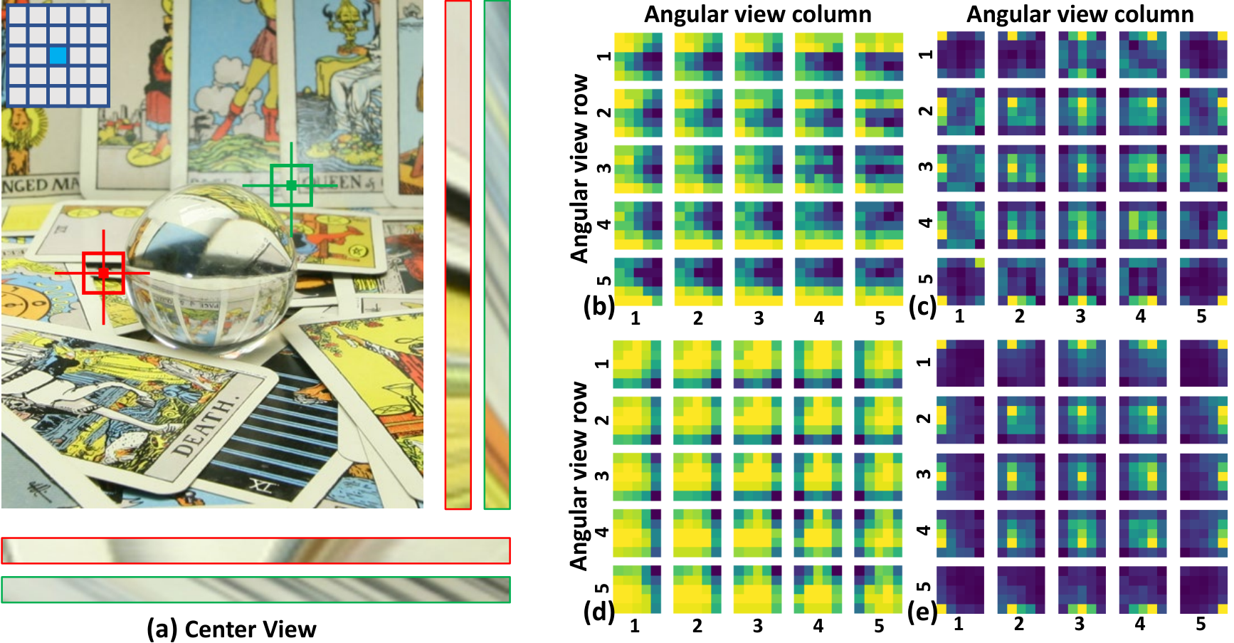
Moreover, we investigate the spatial-aware modeling capability of our angular Transformer by visualizing the local angular attention maps. Specifically, we selected two patches from scene Cards [38], and obtained the attention maps (a 2525 matrix for a spatial location in a 55 LF) produced by the MHSA in the first angular Transformer at each spatial location in the patches. Note that, larger values in the attention maps represent higher similarities between a pair of angular tokens. We then define “local angular attention” by calculating the ratios of similar tokens (with attention scores larger than 0.025) in the selected patches. Finally, we visualize the local angular attention map in Fig. 4 by assembling the calculated attention values according to their angular coordinates. It can be observed in Fig. 4(b) that the attention values in the occlusion area (red patch) are distributed unevenly, where the non-occluded pixels share larger values. It demonstrates that our angular Transformer can adapt to different image contents and achieve spatial-aware angular modeling.
Similarly, we calculate the self-correlation of the feature generated by the LF-InterNet[15] (CNN-based method) in angular dimensions, and the similarity maps of red patch and green patch are shown in Fig. 4(c) and Fig. 4(d), respectively. It can be observed that the view-wise correlation of LF-InterNet is not obvious, i.e., each view has higher similarities with its adjacent views only.
IV-C2 Spatial Transformer
We demonstrate the effectiveness of the spatial Transformer by comparing the performance of model-4 to model-1 and model-6 to model-3. As shown in Table III, model-4 achieves a 0.3 dB improvements in PSNR over model-1. Moreover, when the spatial Transformer is removed from our LFT, model-3 suffers a notable performance degradation (0.080.27 dB in PSNR). That is because, compared to cascaded convolutions, the proposed spatial Transformer can better exploit long-range context information with a global receptive field, and can capture more beneficial spatial information for image SR.
V Conclusion
In this paper, we propose a Transformer-based network (i.e., LFT) for LF image SR. By using our proposed angular and spatial Transformers, the complementary angular information among all the views and the long-range spatial dependencies within each SAI can be effectively incorporated. Experimental results have demonstrated the superior performance of our LFT over state-of-the-art CNN-based SR methods.
References
- [1] Y. Wang, J. Yang, Y. Guo, C. Xiao, and W. An, “Selective light field refocusing for camera arrays using bokeh rendering and superresolution,” IEEE Signal Processing Letters, vol. 26, no. 1, pp. 204–208, 2018.
- [2] S. Jayaweera, C. Edussooriya, C. Wijenayake, P. Agathoklis, and L. Bruton, “Multi-volumetric refocusing of light fields,” IEEE Signal Processing Letters, vol. 28, pp. 31–35, 2020.
- [3] W. Wang, Y. Lin, and S. Zhang, “Enhanced spinning parallelogram operator combining color constraint and histogram integration for robust light field depth estimation,” IEEE Signal Processing Letters, vol. 28, pp. 1080–1084, 2021.
- [4] J. Lee and R. Park, “Reduction of aliasing artifacts by sign function approximation in light field depth estimation based on foreground–background separation,” IEEE Signal Processing Letters, vol. 25, no. 11, pp. 1750–1754, 2018.
- [5] A. Wang, “Three-stream cross-modal feature aggregation network for light field salient object detection,” IEEE Signal Processing Letters, vol. 28, pp. 46–50, 2020.
- [6] Y. Wang, T. Wu, J. Yang, L. Wang, W. An, and Y. Guo, “Deoccnet: Learning to see through foreground occlusions in light fields,” in Winter Conference on Applications of Computer Vision (WACV), 2020, pp. 118–127.
- [7] S. Zhang, Z. Shen, and Y. Lin, “Removing foreground occlusions in light field using micro-lens dynamic filter,” in Proceedings of the International Joint Conference on Artificial Intelligence (IJCAI), 2021, pp. 1302–1308.
- [8] Y. Yoon, H. Jeon, D. Yoo, J. Lee, and I. Kweon, “Light-field image super-resolution using convolutional neural network,” IEEE Signal Processing Letters, vol. 24, no. 6, pp. 848–852, 2017.
- [9] Y. Yuan, Z. Cao, and L. Su, “Light-field image superresolution using a combined deep cnn based on epi,” IEEE Signal Processing Letters, vol. 25, no. 9, pp. 1359–1363, 2018.
- [10] Y. Wang, F. Liu, K. Zhang, G. Hou, Z. Sun, and T. Tan, “Lfnet: A novel bidirectional recurrent convolutional neural network for light-field image super-resolution,” IEEE Transactions on Image Processing, vol. 27, no. 9, pp. 4274–4286, 2018.
- [11] S. Zhang, Y. Lin, and H. Sheng, “Residual networks for light field image super-resolution,” in Proceedings of the IEEE Conference on Computer Vision and Pattern Recognition (CVPR), 2019, pp. 11 046–11 055.
- [12] S. Zhang, S. Chang, and Y. Lin, “End-to-end light field spatial super-resolution network using multiple epipolar geometry,” IEEE Transactions on Image Processing, vol. 30, pp. 5956–5968, 2021.
- [13] J. Jin, J. Hou, J. Chen, and S. Kwong, “Light field spatial super-resolution via deep combinatorial geometry embedding and structural consistency regularization,” in Proceedings of the IEEE Conference on Computer Vision and Pattern Recognition (CVPR), 2020, pp. 2260–2269.
- [14] H. Yeung, J. Hou, X. Chen, J. Chen, Z. Chen, and Y. Chung, “Light field spatial super-resolution using deep efficient spatial-angular separable convolution,” IEEE Transactions on Image Processing, vol. 28, no. 5, pp. 2319–2330, 2018.
- [15] Y. Wang, L. Wang, J. Yang, W. An, J. Yu, and Y. Guo, “Spatial-angular interaction for light field image super-resolution,” in European Conference on Computer Vision (ECCV). Springer, 2020, pp. 290–308.
- [16] Y. Wang, J. Yang, L. Wang, X. Ying, T. Wu, W. An, and Y. Guo, “Light field image super-resolution using deformable convolution,” IEEE Transactions on Image Processing, vol. 30, pp. 1057–1071, 2020.
- [17] G. Liu, H. Yue, J. Wu, and J. Yang, “Intra-inter view interaction network for light field image super-resolution,” IEEE Transactions on Multimedia, pp. 1–1, 2021.
- [18] N. Meng, H. So, X. Sun, and E. Lam, “High-dimensional dense residual convolutional neural network for light field reconstruction,” IEEE transactions on pattern analysis and machine intelligence, 2019.
- [19] A. Dosovitskiy, L. Beyer, A. Kolesnikov, D. Weissenborn, X. Zhai, T. Unterthiner, M. Dehghani, M. Minderer, G. Heigold, S. Gelly, J. Uszkoreit, and N. Houlsby, “An image is worth 16x16 words: Transformers for image recognition at scale,” in Proceedings of the International Conference on Learning and Representation (ICLR), 2021.
- [20] M. Zheng, P. Gao, X. Wang, H. Li, and H. Dong, “End-to-end object detection with adaptive clustering transformer,” arXiv preprint arXiv:2011.09315, 2020.
- [21] N. Carion, F. Massa, G. Synnaeve, N. Usunier, A. Kirillov, and S. Zagoruyko, “End-to-end object detection with transformers,” in European Conference on Computer Vision (ECCV). Springer, 2020, pp. 213–229.
- [22] S. Zheng, J. Lu, H. Zhao, X. Zhu, Z. Luo, Y. Wang, Y. Fu, J. Feng, T. Xiang, P. Torr et al., “Rethinking semantic segmentation from a sequence-to-sequence perspective with transformers,” in Proceedings of the IEEE Conference on Computer Vision and Pattern Recognition (CVPR), 2021, pp. 6881–6890.
- [23] R. Ranftl, A. Bochkovskiy, and V. Koltun, “Vision transformers for dense prediction,” in Proceedings of the IEEE/CVF International Conference on Computer Vision, 2021, pp. 12 179–12 188.
- [24] Z. Wang, X. Cun, J. Bao, and J. Liu, “Uformer: A general u-shaped transformer for image restoration,” arXiv preprint arXiv:2106.03106, 2021.
- [25] J. Cao, Y. Li, K. Zhang, and L. Van Gool, “Video super-resolution transformer,” arXiv preprint arXiv:2106.06847, 2021.
- [26] B. Lim, S. Son, H. Kim, S. Nah, and K. Lee, “Enhanced deep residual networks for single image super-resolution,” in Proceedings of the IEEE Conference on Computer Vision and Pattern Recognition Workshops (CVPRW), 2017, pp. 136–144.
- [27] H. Chen, Y. Wang, T. Guo, C. Xu, Y. Deng, Z. Liu, S. Ma, C. Xu, C. Xu, and W. Gao, “Pre-trained image processing transformer,” in Proceedings of the IEEE Conference on Computer Vision and Pattern Recognition (CVPR), 2021, pp. 12 299–12 310.
- [28] A. Vaswani, N. Shazeer, N. Parmar, J. Uszkoreit, L. Jones, A. Gomez, Ł. Kaiser, and I. Polosukhin, “Attention is all you need,” in Advances in neural information processing systems, 2017, pp. 5998–6008.
- [29] Y. Chen, S. Liu, and X. Wang, “Learning continuous image representation with local implicit image function,” in Proceedings of the IEEE Conference on Computer Vision and Pattern Recognition (CVPR), 2021, pp. 8628–8638.
- [30] W. Shi, J. Caballero, F. Huszár, J. Totz, A. Aitken, R. Bishop, D. Rueckert, and Z. Wang, “Real-time single image and video super-resolution using an efficient sub-pixel convolutional neural network,” in Proceedings of the IEEE Conference on Computer Vision and Pattern Recognition (CVPR), 2016, pp. 1874–1883.
- [31] J. Kim, J. Lee, and K. Lee, “Accurate image super-resolution using very deep convolutional networks,” in Proceedings of the IEEE Conference on Computer Vision and Pattern Recognition (CVPR), 2016, pp. 1646–1654.
- [32] Y. Zhang, K. Li, K. Li, L. Wang, B. Zhong, and Y. Fu, “Image super-resolution using very deep residual channel attention networks,” in European Conference on Computer Vision (ECCV), 2018, pp. 286–301.
- [33] S. Wang, T. Zhou, Y. Lu, and H. Di, “Detail preserving transformer for light field image super-resolution,” in Proceedings of the AAAI Conference on Artificial Intelligence,, 2022.
- [34] M. Rerabek and T. Ebrahimi, “New light field image dataset,” in International Conference on Quality of Multimedia Experience (QoMEX), 2016.
- [35] K. Honauer, O. Johannsen, D. Kondermann, and B. Goldluecke, “A dataset and evaluation methodology for depth estimation on 4d light fields,” in Asian Conference on Computer Vision (ACCV). Springer, 2016, pp. 19–34.
- [36] S. Wanner, S. Meister, and B. Goldluecke, “Datasets and benchmarks for densely sampled 4d light fields.” in Vision, Modelling and Visualization (VMV), vol. 13. Citeseer, 2013, pp. 225–226.
- [37] M. Pendu, X. Jiang, and C. Guillemot, “Light field inpainting propagation via low rank matrix completion,” IEEE Transactions on Image Processing, vol. 27, no. 4, pp. 1981–1993, 2018.
- [38] V. Vaish and A. Adams, “The (new) stanford light field archive,” Computer Graphics Laboratory, Stanford University, vol. 6, no. 7, 2008.
- [39] Z. Wang, A. Bovik, H. Sheikh, and E. Simoncelli, “Image quality assessment: from error visibility to structural similarity,” IEEE Transactions on Image Processing, vol. 13, no. 4, pp. 600–612, 2004.
- [40] X. Glorot and Y. Bengio, “Understanding the difficulty of training deep feedforward neural networks,” in Proceedings of the International Conference on Artificial Intelligence and Statistics (AISTATS), 2010, pp. 249–256.
- [41] D. Kingma and J. Ba, “Adam: A method for stochastic optimization,” Proceedings of the International Conference on Learning and Representation (ICLR), 2015.