Graph Contrastive Learning for Anomaly DetectionThanks:
Bo Chen and Peng Zhang are with Department of Computer Science and Technology, Tsinghua University, Beijing, China, 100084. E-mail: {cb21, zhangp18}@mails.tsinghua.edu.cn,
Jing Zhang and Xiaokang Zhang are with Information School, Renmin University of China, Beijing, China. E-mail:{zhang-jing, zhang2718}@ruc.edu.cn
Yuxiao Dong is with Department of Computer Science and Technology, Tsinghua University, Beijing, China, 100084. E-mail: yuxiaod@tsinghua.edu.cn
Jian Song is with Zhipu.AI, Beijing, China. Email: sxusjj@gmail.com.
Kaibo Xu is with Mininglamp Technology, Beijing, China. Email: xukaibo@mininglamp.com.
Evgeny Kharlamov is with Bosch Center for Artificial Intelligence, Renningen, Germany. Email: Evgeny.Kharlamov@de.bosch.com and University of Oslo, Norway. Email: Evgeny.Kharlamov@ifi.uio.no.
Jie Tang is with Department of Computer Science and Technology, Tsinghua University, and Tsinghua National Laboratory for Information Science and Technology (TNList), Beijing, China, 100084. E-mail: jietang@tsinghua.edu.cn,
*Corresponding author
Thanks:
Abstract
Graph-based anomaly detection has been widely used for detecting malicious activities in real-world applications. Existing attempts to address this problem have thus far focused on structural feature engineering or learning in the binary classification regime. In this work, we propose to leverage graph contrastive learning and present the supervised GraphCAD model for contrasting abnormal nodes with normal ones in terms of their distances to the global context (e.g., the average of all nodes). To handle scenarios with scarce labels, we further enable GraphCAD as a self-supervised framework by designing a graph corrupting strategy for generating synthetic node labels. To achieve the contrastive objective, we design a graph neural network encoder that can infer and further remove suspicious links during message passing, as well as learn the global context of the input graph. We conduct extensive experiments on four public datasets, demonstrating that 1) GraphCAD significantly and consistently outperforms various advanced baselines and 2) its self-supervised version without fine-tuning can achieve comparable performance with its fully supervised version.
Index Terms:
Graph Neural Network, Anomaly Detection, Contrastive LearningI Introduction
Anomaly detection has profound impacts on preventing malicious activities in various applications, such as detecting online review spams [34], financial frauds [50, 28], fake users [11], and misinformation [8, 43]. The most promising development is to utilizing graph structures via machine learning models for distinguishing the anomalies from normal nodes, as graphs can be used for modeling the structural dependencies underlying the data [25, 32, 10].
Recently, the advances of graph neural networks (GNNs) [23, 47, 13] have inspired and empowered various attempts to adopt GNNs for detecting anomalies [32, 10, 42, 50, 18]. The main idea of GNN-based anomaly detection is to leverage the power of GNNs to learn expressive node representations with the goal of distinguishing abnormal nodes from normal ones in the embedding space. Most of the GNN models are based on the inductive bias that two neighboring nodes tend to have the same labels. However, suspicious links between abnormal and normal nodes violate the above assumption, making GNNs produce confusing node embeddings.

To further understand the behavior of anomalies, we take the author ‘‘Jun Lu”, a professor from Yale University, from the published author profile of Google Scholar as a case study by building a graph with papers assigned to him as nodes, and connect two papers with edges if they share the same coauthors, affiliations, or venues.
The goal here is to detect wrongly assigned papers (anomalies), i.e., those are not authored by him.
This anomaly detection problem can be motivated by a news11
1
https://www.universityworldnews.com/post.php?story=
20120807160325397 reported in 2012 that another researcher named “Jun Lu” from Beijing University of Chemical Technology cheated the awards using the papers of “Jun Lu” from Yale. This event caused by the wrongly assigned papers of the same author name implies the importance of anomaly detection. Thus, we illustrate how the wrongly assigned papers can be distinguished from the right ones in Fig. 1.
Fig. 1(a) shows the t-SNE22
2
https://lvdmaaten.github.io/tsne/ projection of each node’s input features—the BERT embedding [9] of its title—with blue as normal nodes and red as abnormal ones.
We observe both abnormal and normal nodes are distributed diversely with abnormal ones being relatively more diverse.
Intuitively, we quantify this observation by computing the similarity between each node and the global context—the average of all node features, which is shown in Fig. 1(b).
It suggests that though having slight overlaps, the two similarity distributions can be clearly distinguished.
Inspired by these observations, we explore whether there is a straightforward way to capture them for distinguishing abnormal nodes from normal ones.
Present Work. In light of the recent progress in contrastive learning [56, 14], we propose to contrast each node with the global context of the input graph. The underlying assumption is that abnormal nodes tend to be more distant from the majority of nodes, namely the graph context, than normal ones. We name the model as GraphCAD, a Graph Contrastive Learning for Anomaly Detection. Specifically, we design the context-aware graph contrastive loss in a supervised manner, i.e., labeled normal and abnormal nodes are treated as positive and negative keys, respectively (Cf. Section II-B), differing it from most existing studies that use graph contrastive learning in a self-supervised pre-training setup [61, 48, 37]. Fig. 1(d) plots the similarity distributions of embeddings generated by GraphCAD compared with that by GCN [23] shown in Fig. 1(c), demonstrating GraphCAD’s striking capacity of separating abnormal nodes from normal ones when considering their distances to the global context of the graph.
In addition to the supervised GraphCAD model, we also extend it in an unsupervised pre-training manner GraphCAD-pre for handling cases with scarce labels. Straightforwardly, we need to synthesize node labels that can be directly used to replace the ground-truth labels in the supervised contrastive loss. To achieve this, we design a strategy to corrupt each part of the original graph by injecting the nodes outside this part.
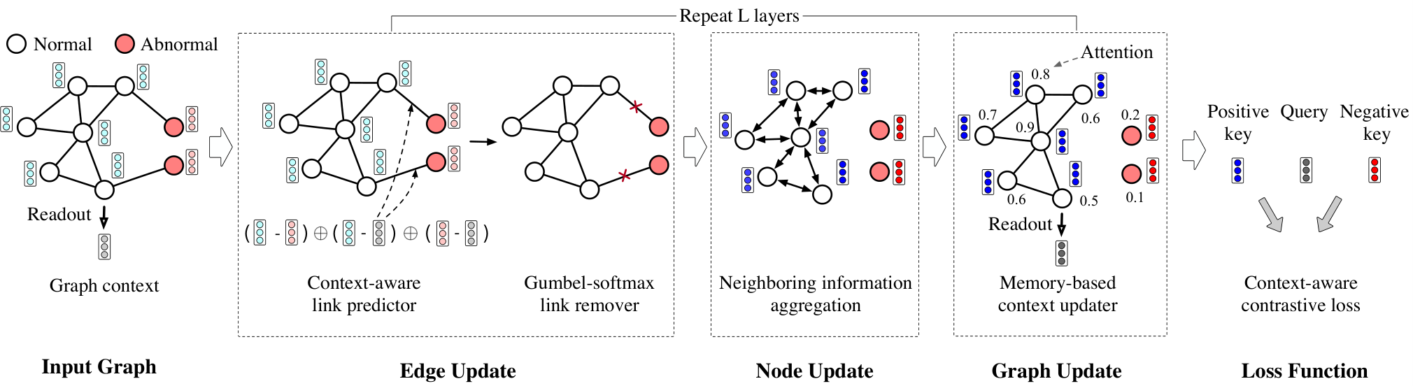
To achieve the contrastive goal, we propose a context-aware GNN encoder with three modules: edge update, node update, and graph update. First, edge update is used to estimate the suspicious likelihood of each link and then update the adjacency matrix by removing the most suspicious links. Then, node update is to update node embeddings by message passing on the updated adjacency matrix. Finally, graph update is designed to update the global context iteratively.
We verify the proposed model by two genres of anomaly detection tasks, i.e., detecting wrongly assigned papers in researchers’ profiles on two academic datasets — AMiner and MAS, and detecting users who give fraudulent ratings on two business websites — Alpha and Yelp. The academic datasets have multiple author profiles where each profile can be viewed as a graph, dubbed as the multi-graph setting. While the business datasets, which have one large graph, are viewed as the single-graph setting. Experiments show that: 1) GraphCAD yields substantial improvements on multi-graph datasets, while presenting subtle but consistent performance gain on single-graph datasets compared with state-of-the-art baselines; 2) the unsupervised GraphCAD-pre is comparable with the fully-supervised GraphCAD. With further fine-tuning, GraphCAD-pre can outperform GraphCAD on most of the datasets. In general, GraphCAD-pre yields consistently better performance than other compared graph pre-training methods. The main contributions are summarized as follows:
- •
We propose the idea of using graph contrastive learning for anomaly detection and present GraphCAD by designing context-aware graph contrastive objective.
- •
We design an effective strategy to yield synthetic labels for extending GraphCAD to unsupervised GraphCAD-pre.
- •
We devise a context-aware GNN encoder via injecting context information to obtain both node and context representations.
- •
We conduct experiments, showing the substantial improvements brought by GraphCAD and GraphCAD-pre.
II GraphCAD
In this section, we first introduce the problem definition of anomaly detection (Section II-A), and then conduct the preliminary observations to verify the motivation of GraphCAD (Section II-A). After that, we propose the learning objective with theoretical guarantees (Section II-B), and further extend the supervised objective to the unsupervised setting (Section II-C). Finally, we introduce the context-aware GNN encoder of GraphCAD and GraphCAD-pre (Section II-D).
II-A The Studied Problem
We define a graph as , where is the set of nodes, denotes the adjacency matrix, and is the corresponding feature vectors with representing the -dimensional feature vector of node . Without loss of generality, we consider as an undirected and single-relational graph, i.e., if there exists an edge between and and otherwise.
Problem 1
Graph-based Anomaly Detection. Given a graph , is the set of node labels with equals to 1 if is abnormal and 0 otherwise. The goal is to learn a function to determine whether a given node is abnormal (1) or normal (0).
To resolve this problem, most existing GNN-based models directly instantiate as a binary classifier [10, 32]. We conduct the following preliminary observations to verify the motivation of the proposed model.
Preliminary Observations. To further verify the motivation of contrasting a node with the global context in Fig. 1, we additionally extract 10,000 authors owning more than 500,000 papers from AMiner33 3 https://www.aminer.org/. Each author profile is treated as a graph with its papers as nodes and connections among papers as edges. Notably, we mainly focus on detecting anomalies in the multi-graph setting in this paper, which is a more challenging and under-explored scenario (Cf. Section 3.2). However, our proposed method can also be instantiated as the single-graph setting. Likewise, the goal here is to detect the wrongly assigned papers (anomalies). For each author, the wrongly assigned papers (anomalies) are labeled by professional annotators or the author themselves. For each paper, we obtain its BERT embedding [9] by its title. Then we calculate the cosine similarity between a pair of papers and average the pairwise cosine similarities of three groups, i.e., Normal and Normal (N-N), ABnormal and ABnormal (AB-AB), and Normal and ABnormal (N-AB). Fig. 2(a) shows the following phenomenon.
- •
Intra-Diversity: The similarities in both N-N and AB-AB are extremely diverse (being scattered within [0.2,0.8]), which is in concert with the case in Fig. 1(a);
- •
Inter-Diversity: The similarities of N-AB are also diverse, and more than 20% abnormal nodes are similar to the normal nodes (y 0.5).
We conjecture this intra-/inter- diversity will degrade the performance of distinguishing anomalies from normal ones by the traditional classifier. To verify this, we investigate the same similarities based on the embeddings generated by GCNs [23] with the binary classification loss, as shown in Fig. 2(b). It demonstrates that although the similarities in N-N increase from [0.2, 0.8] to [0.4, 1.0], the intra- and inter- diversity issues are still severe.
Previous efforts [32, 25] disclose the behavior patterns of anomalies are different from those of normal nodes, based on which they characterize the inductive bias to detect anomalies. However, most of them only focus on modifying the message passing process to reduce propagated noises, while ignoring the limited capability of the binary classification objective when the data distribution is diverse.
Inspired by the case observed in Fig. 1(b), we compute the similarity between each node and the global context---the average of all the node features44 4 The global context is later estimated by the memory-based context updater., and show the average similarities in N-GL and AB-GL in Fig. 2(c). We can see that, compared with Fig. 2(a), although still having overlaps, the two similarity distributions can be distinguished much more clearly. Furthermore, we plot the similarities based on the embeddings generated by GraphCAD in Fig. 2(d). Compared with Fig. 2(c), the resultant embeddings of normal and abnormal ones can be further distinguished.
To this, we empirically verify the motivation of the context-aware contrastive learning method — instead of directly capturing the absolute difference between normal and abnormal nodes, contrasting the relative distances between the node and global context is expected to be a more promising way to address the diversity of node distributions.
II-B Methodology
The basic idea of GraphCAD is to determine a node’s abnormality by contrasting it with the global context of the entire graph. This is motivated by the discovery that there exists a significant difference in the distance to the global context between normal and abnormal nodes. In another words, a node is more abnormal if it deviates farther away from the majority of nodes in the feature space.
In view of this, we distinguish abnormal and normal nodes in the embedding space by the graph contrastive learning (GraphCAD). Specifically, given a graph , we first create a GNN encoder that can output an embedding for each node and also an embedding for the entire graph (global context), i.e., ( with and as the trainable parameters of . We take the graph embedding as the query, a normal node’s embedding as the positive key that matches with , and the embeddings of all the abnormal nodes as the negative keys that don’t match with . For implementation, we use infoNCE [36] in a supervised manner as the concrete loss function such that:
| (1) |
where is the temperature hyperparameter. The objective function is to enforce maximizing the consistency between the positive pairs (normal node, global context) compared with negative pairs (abnormal node, global context).
Compared with the context-aware contrastive learning, the traditional normal-abnormal contrast is a node-wise contrastive pattern, which usually suffers from noisy labels. For example, [21] states that false-negative instances hinder the performance of contrastive learning. On the contrary, the proposed local-global method contrasts each abnormal node with the global context, which can reduce the negative influence of individual noisy labeled nodes.
Why does GraphCAD work? We theoretically prove the effectiveness of the proposed GraphCAD compared with the original cross-entropy loss for classification.
Theorem 1
Let 55 5 We denote random variables using upper-case letters (e.g. , ), and their realizations by the corresponding lower-case letter (e.g. , ). denote the random variable of normal node and denote its marginal distribution, thus . Likewise, we denote the abnormal node by and its marginal distribution by , . Assume and are mutually independent. Then we have: minimizing the contrastive loss in Eq. (1) forms the lower bound of 1) the cross-entropy of the two data distributions and plus 2) the entropy of . Formally,
| (2) |
In view of the two parts in Eq. (2), the contrastive loss is theoretically and analytically more robust than the cross-entropy loss and node-wise contrastive loss because of the following reasons.
First, the local-global contrast can better deal with the diverse abnormal distribution. Theorem 1 shows that the proposed local-global contrastive loss can be decomposed into the cross-entropy between the distribution of the normal node and the abnormal node plus the entropy of the abnormal node. Since the first term links to the node-wise contrastive loss [5], which is also proved to be the cross-entropy between the predicted labels and the ground truth labels [5], the proposed local-global contrastive loss has an additional entropy of the abnormal node compared with the cross-entropy loss. Such additional entropy, acting as a normalization constraint, makes the distribution of learned abnormal node features spread uniformly as much as possible in the feature space. Thus it can better deal with the diverse feature distributions, especially the abnormal diverse distribution, which can be exactly observed in the anomaly detection datasets (Cf. Fig. 1).
Second, the local-global contrast can reduce the label-imbalance issue. Maximizing the additional entropy of abnormal nodes also augments informative features of the abnormal nodes, reducing the label imbalance issue of the abnormal nodes against the normal nodes to some degree. The common assumption in anomaly detection is that the abnormal node is the minority class, because the number of abnormal nodes is much smaller than normal ones. Thus, traditional anomaly detection methods usually suffer from the class imbalance issue. To alleviate it, data augmentation techniques for generating pseudo-labels of the minority classes [3], up-sampling or down-sampling techniques for re-balancing the class distribution [4], etc., are proposed. The core insight is to augment the information of minority classes, which can balance the training bias between majority classes and minority classes. Such the balancing technique somehow agrees with the optimizing goal of the second part of Eq. (2), which augments informative features of the abnormal nodes to balance the training bias.
Proof of Eq. (2). Let = , where , then we have the normal node embedding matrix , where is the number of normal nodes. Likewise, we define = and the abnormal node embedding matrix with the node number . Note that, . Let be a deterministic readout function on graphs. Without loss of generality, we assume . Thus . From Eq. (1), we can derive
| (3) | |||||
where the “alignment” term pulls the distances between the normal nodes and the global context closer, and the “uniformity” term pushes the distances between the abnormal nodes and the global context away [52].
Since , we get
| (4) |
Note that and learned by Inter-/Intra- Diversity observations, the similarity scores between normal nodes is predominant and usually large, that is, the term is naturally large, thus the main challenge lies in optimizing the “uniformity”. Asymptotically, suppose the normal node pairs are perfectly aligned, i.e., , minimizing Eq. (3) is equivalent to optimizing the second term, i.e.
| (5) |
where the first inequality follows the Jensen Inequality based on the concavity of the log function, namely .
As and are mutually independent and the data samples from either or follow i.i.d. assumptions, minimizing the last equation of Eq. (5) is equivalent to minimizing both the sum of similarities between normal and abnormal node embeddings and the sum of the similarities between abnormal and abnormal node embeddings, i.e.
| (6) |
where the second equality is obtained by first applying exponent to the each of similarity score, and then re-scaling the expectation of the similarity scores in the logarithm form. Notably, the second equation holds true under the minimization optimization circumstance. Moreover, inspired by the entropy estimation operation in [52], the last equality can be viewed as a resubstitution entropy estimator of [1] via a von Mises-Fisher (vMF) kernel density estimation (KDE), where is the normalization constant and denote the resubstitution entropy estimator.
The results reveal that minimizing Eq. (1) is equivalent to maximizing the cross-entropy between the two data distributions, and and the entropy of .
Connection to Existing Graph CL Frameworks. GraphCAD, that performs contrastive learning in a supervised manner, differs from existing graph contrastive learning frameworks for GNN pre-training, such as GCC [37], DGI [48], GraphCL [61], because most of them are self-supervised and the contrastive instances should be constructed from the unlabeled data. For example, in GCC [37], given the embedding of a randomly sampled ego-network of a node as the query, the positive key is the embedding of another sampled ego-network of the same node, and the negative keys are those sampled from other nodes. In DGI [48], given the entire graph embedding as the query, the positive key is the embedding of a node in it, and the negative keys are those of the same node after permutating the graph. GraphCL [61] further contrasts between different graph augmentations. Given the embedding of a graph as the query, the positive key is the embedding of the graph augmented from the same graph, while the negative keys are those from different graphs. In contrast, in our objective for anomaly detection, given the graph embedding as the query, the positive and the negative keys are constrained to the normal and abnormal nodes respectively. In light of this, GraphCAD is a kind of supervised contrastive learning [22].
II-C GraphCAD-pre for Unsupervised Settings
Sufficient labels of anomalies are often arduously expensive to obtain, which is the bottleneck of most anomaly detection scenarios. Therefore, we further extend GraphCAD as an unsupervised pre-training model (GraphCAD-pre) to handle real-world applications with scarce labels.
We present a pre-training strategy for tackling the label scarce problem in anomaly detection. Inspired by the idea of context-aware contrastive objective, we propose to construct pseudo anomalies via corrupting the original graph. Considering one small part of the original graph, we inject nodes outside this part into it. The underlying assumption is that as nodes in different parts of the graph follow different distributions [37, 48], they can serve as the pseudo anomalies to the context of the small part of the original graph. Formally, a corrupt graph is defined as follows:
Definition 1
Corrupt Graph. Given a graph , we break it into parts . For each part , a corrupt graph is created by injecting a set of nodes from the parts except , i.e., , thus the corrupt nodes are the union of and , i.e., . The corrupt adjacency matrix of is obtained by slicing using the indexes in .
Fig. 3 illustrates a toy example of creating corrupt graphs. There are different ways for breaking the input graph into multiple parts w.r.t various graph distributions, which can be summarized into two categories:
- •
Single-Graph: If the original graph is a single graph, we partition it into multiple parts using clustering algorithms. Specifically, we perform the K-means algorithm based on the initial features , and determine the size of the clusters via finding the elbow point of inertia, a well-adopted clustering metric (Cf. Section III-C).
- •
Multi-Graphs: If the original graph is composed by multiple sub-graphs, without partition, these sub-graphs can be naturally viewed as different parts of the original graph.
For the corrupt graphs with injected nodes as pseudo anomalies and original nodes as normal ones, we can directly optimize the context-aware graph contrastive loss defined in Eq. (1), which can be further fine-tuned on the target graph if the ground-truth labels are available.
Connection to Graph Pre-Training Frameworks. Existing graph pre-training methods offer limited benefits to anomaly detection. For example, GAE [24] reconstruct the adjacency matrix under the local proximity assumption, which is hurt by suspicious links. GCC [37] maximizes the consistency between the sampled ego-networks of the same node compared with those sampled from different nodes, such feature consistency assumption cannot explicitly help distinguish the abnormal nodes from the normal ones. DGI [48], which contrasts a node with the whole graph, is akin to the contrastive objective of GraphCAD-pre, while the negative instances are addressed differently. In DGI, given a graph as the context, positive and negative nodes are convolved and represented in independent graphs before contrasting. But in GraphCAD-pre, negative nodes sampled from other graphs are injected and may link to normal nodes in the corrupted graph, which increases the difficulty to distinguish normal and abnormal nodes during training, and thus improves the discrimination ability of the model. Essentially, DGI focuses more on representing the normal pattern while GraphCAD-pre additionally reinforces the differences of the anomalies from the normal pattern.
II-D The GNN Encoder of GraphCAD
II-D1 Overview
To optimize the context-aware contrastive objective in Eq. (1), we design the edge update, node update, and graph update modules in the GNN encoder of GraphCAD. First, Edge update is to estimate the likelihood of each link being a suspicious one and then remove the suspicious ones. Then, node update is to update node embeddings by message passing on the updated adjacency matrix. Finally, the global context is updated via graph update. The three modules are executed at each graph convolution layer successively. After -layer forwards, the context-aware contrastive objective is optimized. The framework is illustrated in Fig. 4.
II-D2 Edge Update
We define suspicious links as the ones that connect nodes with opposite labels. For example, almost every fraudster in business websites can be linked to some benign users by the commonly rated products. Such suspicious links violate the homophily assumption between neighbors—two neighboring nodes tend to have similar features and same labels—and impact the performance of the traditional message-passing along with the suspicious links.
Although many attempts have been made to detect such suspicious links [63, 10], they merely predict the likelihood based on the linked node features regardless of the node labels. Differently, we additionally model the relative distance between nodes and the global context . The promise here is the distance can serve as implicit labels to guide the model to remove suspicious links — those connected by the nodes with distinguished distance to the global context.
Context-Aware Link Predictor. The link predictor accepts the representations of two linked nodes and as the input, and then estimates the linkage likelihood between node and by:
| (7) | |||
where is the concatenation operator and MLP is a projection layer with a sigmoid activation function to normalize the likelihood into [0,1]. explicitly denotes the similarity of two nodes, while , the distance from to the global context, implicitly indicates that two nodes—even if their local features are slightly different—can be highly probably linked given their relative positions to the global context are similar. The ablation studies in Section 3.2 empirically prove the effectiveness of this context-aware link predictor.
To accelerate the optimization of the link predictor, we optimize the prediction loss in addition to the contrastive objective in Eq. (1). Specifically, we treat links between normal nodes as positive ones and suspicious links as negative ones. The prediction loss is defined as
| (8) |
which acts as the constraint to directly maximize probabilities of normal links and minimize these of suspicious ones.
Gumbel-softmax Link Remover. We remove the suspicious links to reduce their negative influence thoroughly by employing the Bernoulli approximation, the binary case of the Gumbel-softmax reparameterization trick [33, 19] to resolve the discrete non-differentiable problem. Specifically, we define the indicator matrix , and for the link likelihood , we decide whether to keep the link or not by the following equation:
| (9) |
where Bernoulli (p) is the Bernoulli approximation with the probability p to keep the link, is the temperature hyper-parameter to control the sharpness of the sampling process (the lower is, the more links will be kept), and is the Gumbel noise for reparameterization. In the forward process, we sample according to Eq. (9) to obtain . In the backward process, a straight-through gradient estimator [3] is employed to pass the gradients to the relaxed value instead of the discrete value .
Edge Residual. Recently, RealFormer [15] verifies the effect of the residual connection of attention scores. Inspired by this, we perform the residual connection of the original edge likelihood and the estimated edge likelihood to smooth the edge evolution as follows:
| (10) |
where is a learnable parameter to balance the weight from the last layer and the estimated weight , and denotes the Hadamard product.
II-D3 Node Update
Updating node embeddings can be divided into an AGGREGATION and a COMBINE operation:
| (11) | |||||
| (12) |
where Eq. (11) is to aggregate the neighboring messages of the last layer based on the updated adjacency matrix and Eq.(12) is to combine the aggregated information with the concerned node. Generally, the two operations are flexible enough to fit any GNNs. Experiments in Section III have investigated several concrete functions.
II-D4 Graph Update
Straightforwardly, we can perform sum, max, or average pooling of all the nodes to update the global context. However, they do not distinguish the normal and abnormal nodes, which results in an inaccurate global context. To alleviate it, we introduce a memory buffer to register the global context of the last layer, based on which we calculate the contribution of each node to the global context. The assumption is a node that is deviated from the current global context should be weakened in the next update step. Such the memory-based mechanism has been successfully applied to general computation machines [2, 54]. Formally,
| (13) | |||
First, we compute the attention for each node based on its cosine similarity with the memory vector. Then we update the global context by weighted aggregating different nodes and update the memory vector . Such a memory-based graph update strategy can get rid of the negative influence of the abnormal nodes on the “positive” global context as much as possible.
Initialize the trainable parameter of ;
repeat 1
Node update to get the node embeddings: .
Graph update to get the global context:
Compute the loss function in Eq. (14).
Update by ;
until Converges; 4
II-E Training and Inference
In each epoch, we optimize both the context-aware contrastive loss in Eq. (1) and the link predictor constraint loss in Eq. (8) as follows:
| (14) |
where is a balanced hyper-parameter. We empirically set as 0.2 in our model. Algorithm 1 outlines the training process. During inference, for node to be predicted, instead of directly predicting a binary label, we estimate its abnormality score by computing the cosine similarity between its embedding and the graph embedding of the final layer (the lower, the more anomalous).
II-F Complexity
The time complexity of GraphCAD is the same order of magnitude as the vanilla GNN. Because on top of the node update step of GNN, GraphCAD adds two additional efficient steps, edge update, and graph update. The time complexity of edge update in layer is , where is the number of edges and is the embedding size in layer . The time complexity of graph update in layer is , where is the number of nodes. Since the embedding size is far smaller than the number of nodes or edges, the time complexity of GraphCAD grows linearly with the graph scale, which is the same as the vanilla GNN.
III Experiment
In this section, we perform two major experiments to verify the performance of the supervised GraphCAD and the unsupervised GraphCAD-pre respectively on two genres of anomaly detection applications. All the codes and the datasets are online now66 6 https://github.com/THUDM/GraphCAD.
| Datasets | Multi-graph | Single-graph | ||||||||||||
|---|---|---|---|---|---|---|---|---|---|---|---|---|---|---|
| AMiner | MAS | Alpha | Yelp | |||||||||||
|
|
|
|
| ||||||||||
| #Total Links | 12,669,793 | 2,543,833 | 24,186 | 3,846,979 | ||||||||||
| #Graphs | 1,104 | 2,098 | 1 | 1 | ||||||||||
| Average #nodes | 174 | 56 | - | - | ||||||||||
| Average #links | 11,476 | 1,212 | - | - | ||||||||||
| #Relation | 3 | 2 | 2 | 3 | ||||||||||
| Concentration | 0.0063 | 0.0075 | 0.0088 | 0.0003 | ||||||||||
| Normal links % | 97.23 | 97.00 | - | 77.30 | ||||||||||
III-A Experimental Setup
Datasets. We evaluate the proposed model for detecting the wrongly assigned papers in researchers’ profiles on two academic datasets and detecting users who give fraudulent ratings on two business websites. The academic datasets are both multi-graph datasets and the business datasets are both single-graph datasets. Table I shows the statistics.
- •
AMiner: is a free online academic system77 7 www.aminer.org collecting over 100 million researchers and 260 million publications [46, 62]. We extract 1,104 online researchers’ profiles, then for each profile, we build a graph by adding papers as nodes and creating a link between two papers if they share the same coauthors, venues or organizations The wrongly assigned papers are provided by human annotators.
- •
- •
Alpha [26]: is a Bitcoin trading platform. A single graph is created by adding users as nodes and the rating relationships between users as links. Benign users are the platform’s founders or users who are rated positively. Fraudsters are the users who are rated negatively by the benign users.
- •
Yelp [39]: is a platform for users to rate hotels and restaurants. A single graph is created by adding spam (abnormal) and legitimate (normal) reviews filtered by Yelp as nodes. The links are created between two reviews if they are posted by the same user, on the same product with the same rating, or in the same month.
For the two multi-graph academic datasets, we use the paper title embedded by BERT as the initial feature for each node. For Yelp, we leverage a sparse matrix of 100-dimension Bag-of-words initial features for each node [10]. For Alpha, since we do not have the side information of nodes, we conduct eigen-decomposition on the graph Laplacian s.t. with as the identity matrix, as the degree matrix, and use the top eigenvectors in U [49] as the initial 256-dimensional features for each node.
| Model | Multi-graph | Single-graph | ||||||
|---|---|---|---|---|---|---|---|---|
| AMiner | MAS | Alpha | Yelp | |||||
| AUC | MAP | AUC | MAP | AUC | MAP | AUC | MAP | |
| Graph Neural Networks | ||||||||
| GCN | 75.68 | 59.28 | 78.44 | 63.89 | 82.12 | 78.09 | 70.85 | 29.18 |
| GAT | 74.97 | 59.87 | 78.25 | 62.75 | 78.45 | 76.32 | 75.28 | 32.11 |
| GSAGE | 73.01 | 60.51 | 76.55 | 62.12 | 79.23 | 75.14 | 76.34 | 34.12 |
| GIN | 74.28 | 57.75 | 75.62 | 59.96 | 87.39 | 86.79 | 76.67 | 34.60 |
| Graph-based Anomaly Detection Models | ||||||||
| LogisticReg | 62.49 | 33.68 | 73.67 | 56.64 | 71.88 | 72.43 | 67.74 | 26.27 |
| GeniePath | 76.18 | 50.67 | 81.93 | 65.66 | 75.02 | 68.89 | 76.78 | 33.67 |
| GraphConsis | 71.37 | 52.21 | 76.67 | 60.25 | 86.99 | 86.63 | 70.27 | 26.64 |
| CARE-GNN | 77.74 | 55.38 | 80.01 | 66.98 | 84.26 | 85.20 | 77.14 | 36.84 |
| GraphCAD | 89.84 | 78.73 | 87.62 | 75.18 | 90.53 | 91.20 | 79.64 | 37.15 |
III-B Evaluation of GraphCAD
Baselines. We compare GraphCAD with four general GNNs models, including GCN [23], GAT [47], GraphSAGE [13], and GIN [58], and three specific GNN models for anomaly detection, i.e., GeniePath [31], GraphConsis [32], and CARE-GNN [10], which are further introduced in Section IV. Other GNN-based anomaly detection models such as GAS [27], FdGars [51], Semi-GNN [50], and Player2Vec [63], are empirically proven to be less powerful than the adopted baselines, thus are ignored in the experiments. We additionally compare with logistic regression by injecting top eigenvectors as features to perform node classification.
| Model | Multi-graph (GCN) | Single-graph (GIN) | ||||||
|---|---|---|---|---|---|---|---|---|
| AMiner | MAS | Alpha | Yelp | |||||
| AUC | MAP | AUC | MAP | AUC | MAP | AUC | MAP | |
| GraphCAD | 89.84 | 78.73 | 87.62 | 75.18 | 90.53 | 91.20 | 79.64 | 37.15 |
| Variant Loss Functions | ||||||||
| + CE_loss | 80.30 | 61.02 | 81.53 | 67.42 | 88.64 | 89.10 | 79.18 | 37.05 |
| Variant Edge Update Strategies | ||||||||
| - LP_constraint | 89.36 | 78.57 | 87.25 | 74.56 | 89.70 | 90.55 | 78.63 | 35.62 |
| - Global Info. | 88.67 | 77.13 | 86.78 | 73.48 | 89.93 | 90.63 | 78.61 | 35.20 |
| - Edge Update | 88.21 | 76.97 | 86.34 | 71.54 | 89.69 | 89.86 | 78.51 | 35.19 |
| Variant Node Update Strategies | ||||||||
| 89.84 | 78.73 | 87.62 | 75.18 | 85.07 | 87.09 | 73.33 | 30.64 | |
| 89.00 | 77.98 | 86.30 | 72.75 | 83.26 | 86.37 | 72.87 | 29.91 | |
| 87.84 | 75.26 | 82.86 | 68.52 | 86.54 | 87.07 | 76.52 | 33.28 | |
| 89.04 | 77.02 | 83.39 | 67.46 | 90.53 | 91.20 | 79.64 | 37.15 | |
| Variant Graph Update Strategies | ||||||||
| + Avg Pooling | 89.01 | 77.66 | 86.39 | 72.73 | 89.02 | 89.57 | 78.70 | 34.55 |
| + Sum Pooling | 86.95 | 72.09 | 86.45 | 73.98 | 88.01 | 86.69 | 76.79 | 34.11 |
| + Max Pooling | 80.91 | 61.97 | 84.06 | 70.52 | 89.25 | 88.56 | 78.54 | 33.96 |
Setup. For the multi-graph datasets, i.e., AMiner and MAS, we extract 70% graphs as the training set, 10% as the validation set, and 20% as the test set. During training, we perform GraphCAD on each graph following Algorithm 1. For testing, we rank nodes based on the cosine similarities between their node embeddings and the corresponding graph context in an ascending order, then we evaluate AUC and MAP of each graph and average the metrics of all test graphs as the final metrics. For the single-graph datasets, i.e. Alpha and Yelp, we also extract 70% of labeled nodes from the single graph as the training data, 10% as the validation set, and 20% as the test set. We perform GraphCAD on the single graph, and evaluate AUC and MAP for the ranked nodes in the test data. Notably, for GraphConsis and CARE-GNN whose inputs are the graph with multi-relation links, we use its multi-relation information, while GraphCAD merges multi-relation links between two nodes into single-relation links. We run 5 trials and report the mean results.
Implementation. For GraphCAD , the number of layers is empirically set as 2, the temperature hyperparameter is set as 0.1 in Eq. (1), and is set as 0.6 in Eq. (9). We use Adam with learning rate 1 for training. The learning rate is set as the initial value over the first 10% steps, and then linearly decay to 1/10 of the initial value.
For the GCN, GAT, GraphSAGE, and GIN, We leverage the implementations provided by Pytorch Geometric99 9 https://github.com/rusty1s/pytorch_geometric, and set the number of convolutional layers as 2 for all general GNNs. For GeniePath, GraphConsis, and CARE-GNN, we use the authors’ official codes with the same training settings. The data format is transformed appropriately to fit their settings. All models are running on Python 3.7.3, 1 NVIDIA Tesla V100 GPU, 512GB RAM, Intel(R) Xeon(R) Gold 5120 CPU @ 2.20GHz.
Overall Results. Table II presents the performance of GraphCAD and all the comparison methods on four datasets. We can see that, GraphCAD substantially improves over all other baselines, +2.5-27.35% in AUC and +0.31-28.06% in MAP, on all the datasets. Among all the baselines, logistic regression performs the worst as it only leverages the structural information and does not apply graph convolution to integrate neighbor messages. None of the specific graph-based anomaly detection methods can keep the advantage over the general GNNs on all the datasets. For example, GraphConsis [32] performs worse than GIN [58] on AMiner. The highlighted results in the table are from GraphCAD, which adopts the context-aware contrastive objective and the three-stage GNN encoder, performing stably the best over all the datasets.
Ablation Studies. To this end, there have two major differences: the context-aware contrastive objective and the three-stage GNN encoder between GraphCAD and other baselines. Thus we conduct the ablation studies to verify the efficacy of different components in GraphCAD. The four main model variants are presented as follows, and the results are illustrated in Table III.
Node Update Strategies. From Table III, we can see that GraphCAD with various node update strategies outperforms other baselines in most cases, which suggests the superiority of context-aware contrastive objective and the three-stage GNN encoder.
We also observe that different strategies have the performance gap, with less than 6% in AUC and 7% in MAP. On the multi-graph datasets, GraphCAD performs the best with the mean AGGREGATION and the concatenation COMBINE strategies in GCN [23], while on the single-graph datasets, it performs the best with the sum AGGREGATION and the concatenation COMBINE strategies in GIN [58]. Obviously, the trend of performance changes over different node update strategies is akin to that of general GNNs, as shown at the top of Table II. Thus we conjecture the instability is mainly due to the intrinsic traits of the node update strategy in GNNs.
Thus, unless stated otherwise, we only conduct experiments of GraphCAD with the best node update strategy, that is, GCN on the multi-graph datasets and GIN on the single-graph datasets, in the remaining parts.
The Contrastive Loss Function. From Table III, we see that the performance gain of GraphCAD over +CE_loss on the multi-graph datasets (+6.09-9.54% in AUC and +7.76-17.71% in MAP) is much higher than that on the single-graph datasets (+0.46-1.89% in AUC and +0.60-2.10% in MAP). Such results empirically validate Theorem 1 that the context-aware contrastive objective is more resilient than cross-entropy in terms of the generation capacity. Since the abnormal node distributions in different graphs are usually quite different, the multi-graph setting presents much more diverse abnormal distributions than the single-graph setting. Thus optimizing the entropy of abnormal nodes take a critical role to learn a more generalized model across various graphs. What’s more, our proposed context-aware contrastive loss performs slightly better than CE_loss in the single-graph datasets, which shows that our method can tackle the class imbalance issue to some degree.
Context-aware GNN Encoder. GraphCAD w/ CE_loss outperforms other state-of-the-art baselines by up to 17.81% AUC, which elucidates the powerful representation capability of the proposed context-aware GNN encoder. The improvements can give credit to two perspectives: the context-aware edge update and the memory-based global update. Thus, We further verify the effectiveness of each component.
Edge Update Strategies. GraphCAD w/o LP_constraint performs slightly worse than GraphCAD, denoting link prediction loss can not only accelerate the optimization of link predictor but also contribute to the overall improvement.
GraphCAD w/o Global Info. underperforms GraphCAD, revealing the context-aware link predictor that incorporates the distance to the global context as the implicit supervision, can benefit the suspicious link prediction.
Compared with above two variants, GraphCAD w/o Edge Update performs the worst (-0.84-1.63% in AUC), verifying the efficacy of the proposed edge update mechanism. However, the performance enhancement brought by the edge update is not significant. We speculate the norm links which connect the nodes of the same labels occupy the majority of all the links (e.g., 90.5% on AMiner and 84.4% on MAS in Table. I). Thus, removing the small amount of suspicious links by the link predictor can only exert limited effect. To verify this, we select the hard instances, i.e., the abnormal nodes that connect at least 1010 10 Empirically, is set as 1 in MAS and 3 in Alpha respectively. normal nodes, from both MAS and Alpha, and re-evaluate the variants on filtered datasets. From Fig. 5(a), we can see that GraphCAD significantly outperforms w/o Edge Update by 3.12% and 2.04% AUC on the two datasets, respectively. The results indicate that the negative influence of the suspicious links can be effectively reduced by the edge update step.
Global Update Strategies. The proposed memory-based global context update mechanism performs the best, which improves 0.83-8.93% AUC and 1.07-16.76% MAP over other variant mechanisms. Because the memory that records the global context of the last layer can help estimate the contribution of each node in the current layer, thus it will benefit the generation of precise global context in the current layer.
| Model | AMiner | MAS | Performance Drop | |
|---|---|---|---|---|
| AMiner | w/ CL | 89.84 | 87.70 | 2.14 |
| w/ CE | 80.30 | 77.05 | 3.25 | |
| MAS | w/ CL | 84.41 | 87.62 | 3.21 |
| w/ CE | 74.15 | 81.53 | 7.38 | |
Transfer Learning. To further investigate the robustness of context-aware contrastive loss compared with cross-entropy objective, we train GraphCAD and its variant w/ CE_loss on AMiner/MAS and evaluate them on MAS/AMiner1111 11 Since the feature initialization process and the embedding dimension of Alpha and Yelp are obviously different from each other, we only conduct the transfer learning experiments between AMiner and MAS.. As shown in Table IV, the performance drop of GraphCAD (-2.14-3.21% in AUC) is substantially less than that of w/ CE_loss (3.25-7.38% in AUC) under the setting of transfer learning, which shows the superior robustness ability of the context-aware contrastive objective compared with the cross-entropy objective.
III-C Evaluation of GraphCAD-pre
Baselines. We compare GraphCAD-pre with the state-of-the-art graph pre-training models, including GAE [24], GPT-GNN [17], GraphCL [61], and the graph pre-training models tailored for anomaly detection, DCI [53], ANEMONE [20], CoLA [30], in the unsupervised setting. GAE is to preserve the structural correlations via reconstructing the vertex adjacency matrix. In addition to the structural correlations, GPT-GNN preserves the attribute interplays via predicting the masked attributes. GraphCL maximizes the mutual information of two instances of the same graph obtained by graph data augmentation. DCI [53] is a cluster-based version of DGI, which maximizes the fine-grained mutual information between the embeddings of a cluster and the nodes within it and is proved to be effective for graph anomaly detection. ANEMONE and CoLA both underperform the proposed GraphCAD-pre. Although ANEMONE and CoLA propose a similar node to sub-graph contrast learning, they sample the sub-graphs by the local random walking algorithm instead of the global clustering algorithm in GraphCAD-pre. The latter can result in more diverse normal samples that are more difficult to be distinguished. On the contrary, the former ignores such difficult normal samples during training, which will reduce the model generalization. For a fair comparison, all the pre-training models adopt the same GNN encoder as GraphCAD.
Datasets. In the online AMiner system, we hide the labeled 1,104 graphs in Table I and extract additional 4,800 corrupt graphs from it. According to the multi-graph corrupting strategy in Section II-C, we first build a single large paper graph for the whole extracted AMiner dataset and then divide it into multiple graphs according to the ownership of papers to different researchers. For each graph, we corrupt it by injecting the papers from other researchers’ graphs as the anomalies with a certain corrupt ratio of 15%, i.e., the ratio between the number of injected nodes with the number of existing nodes in the graph. The links in the original graph are kept between the nodes in corrupt graphs. Then we build the MAS corrupting graph dataset in the same way.
For the single-graph datasets, Alpha and Yelp, we first cluster it into sub-graphs by classic K-means algorithm based on their input features. We perform the clustering algorithm based on the feature information instead of the structure information, because structural information is more preferred to be tampered than the feature information by the abnormal users. Although the abnormal users might perform both the attribute abnormal behaviors which result in the corrupted features and the abnormal structural behaviors which result in the suspicious links between users, the latter can produce a more negative impact on the whole graph. For example, in social network, a rumor monger usually disguises themselves as regular users by building connections with regular users and dispersing the disinformation via the connections. Thus, identifying suspicious linkages between normal and abnormal ones is more crucial in graph anomaly detection. In light of this, it is inappropriate to split the graphs by the structure information that is highly probably polluted by the suspicious links. We didn’t try to split the graph of Alpha by the feature information, as it is unavailable in the dataset.
The within-cluster correlation is measured by sum-of-squares criterion, namely inertia1212 12 https://scikit-learn.org/stable/modules/clustering.html#k-means, estimated by , where is the embeddings of -th cluster center and is disjoint clusters. To automatically set a proper , we leverage the Elbow Methods to choose the elbow point of inertia, i.e, to locate the optimal at which the trend of inertia changes from steep to stable (Cf. Fig. 7). Finally, the graph size is set as 20 on Alpha and 30 on Yelp.
Setup. Without any labeled data (0% labeled data), we train GraphCAD-pre and the baselines on the corrupt graphs and evaluate them on the same test set as the supervised GraphCAD. Then we also explore the few-shot learning settings, i.e., we further fine-tune the pre-trained models when given a proportion of labeled data.
Implementation. For GraphCAD-pre, we follow the same setting as GraphCAD. For GAE, DCI, GPT-GNN, and GraphCL, we use the authors’ official codes with the same training settings. Note that, for GraphCL, we try all the graph augmentation methods defined in the paper and and select the sub-graph augmentation that achieves the best performance in the test set without fine-tuning.
Overall Results. Fig. 6 shows the pre-training and fine-tuning performance of all the comparison methods given different percentage of labeled data on four datasets. From the results, we see that GraphCAD-pre (blue line) fine-tuned on 0%, 10%, and 60% labeled data is comparable with the fully-supervised GraphCAD (black dashed line) on AMiner, MAS, and Alpha respectively. What’s more, when GraphCAD-pre is fined-tuned on all the labeled data, it even outperforms GraphCAD by 1.72%, 2.19%, and 1.04% in AUC on AMiner, MAS, and Alpha respectively, which reveals the effectiveness of the proposed pre-training framework.
Our model also outperforms all the baselines when whatever percentage of labeled data is provided. GAE and GPT-GNN focus on reconstructing the links in the graphs. GraphCL aims to capture the normal distribution of the whole graphs. The objective of them is a little far away from anomaly detection. DCI performs the best among all the baselines. Given the global context as the query, DCI aims to contrast between the nodes within the sub-graph (normal nodes) and those from other sub-graphs (abnormal nodes). The objective is similar to GraphCAD-pre, but different from the corrupted graphs by GraphCAD-pre, the anomalies in DCI are thoroughly disconnected from the normal nodes and are independently embedded in other graphs, which may reduce the learning difficulty of the pseudo labels compared with the ground-truth labels. Both ANEMONE and CoLA under-perform the proposed GCCAD-pre. Although ANEMONE and CoLA propose a similar node to sub-graph contrast learning, they sample the sub-graphs by the local random walking algorithm instead of the global clustering algorithm in GCCAD-pre. The latter can result in more diverse normal samples which are more difficult to be distinguished. On the contrary, the former ignores such difficult normal samples during training, which will reduce the model generalization.
We also observe that on Yelp, none of pre-training models achieve prominent performance without any labeled data. On one hand, as shown in Table I, because of the smallest concentration, Yelp is the most diverse dataset, which prevents GraphCAD-pre, DCI, and GraphCL from discovering the proper normal pattern. On the other hand, since the ratio of the suspicious links on Yelp, 22.70%, is the largest among the datasets, GAE and GPT-GNN that target at preserving the link homophily will wrongly reconstruct those noisy links. However, GraphCAD-pre still performs best compared with other pre-training models on the most of the percentage of labeled data is provided, which implies the ability of GraphCAD-pre to distinguish the normal nodes from the abnormal ones.
Corrupt Ratio. Fig. 5(b) presents the correlation between the ratio of the injected nodes (corrupt ratio) and the performance of GraphCAD-pre on AMiner and Alpha without fine-tuning. The results show that the best performance is achieved when about 15% of abnormal nodes are injected. The corrupt ratio is set in the same way as other datasets.
Clustering Number. Fig. 7 presents the correlation between the graph (cluster) number and the inertia gap between and on Alpha and Yelp. The optimal that achieves the best performance of GraphCAD-pre without fine-tuning are marked as red. We observe that GraphCAD-pre performs the best when (red) is approximately around the elbow point where the trend of inertia changes from steep to stable. Although we choose the elbow points on Yelp, Yelp is so diverse that none of the graph pre-training methods can achieve desired performance.
Features for Clustering. We compare the effect of the clustering algorithm by the structure information or feature information on the pre-training performance. We perform K-means on the graph of Yelp by the structure information, and the result is much poorer than clustering by the feature information (i.e., 12.56% versus. 14.17% in terms of MAP), which indicates the more noisy structural information hampers the clustering as well as the pre-training performance.


IV Related Work
IV-A Graph-based Anomaly Detection
Graph neural networks have been studied to detect anomalies in various domains, such as detecting review spams in business websites [10, 27, 32, 29], rumors in social media [4, 55, 59], fake news [40, 35], financial fraud [31, 57, 38], insurance fraud [28], and bot fraud [60]. Most of them target how to design a proper aggregator that can distinguish the effects of different neighbors and reduce the inconsistency issue [32] during message passing. For example, GAS [27] adopts the vallina GCN [23]. SemiGNN [50] and Player2Vec [63] apply attention mechanisms to assign low weights to suspicious links. To thoroughly reduce the negative influence of the suspicious links, several attempts [12, 32] have been made to remove the suspicious links before graph convolution. CARE-GNN [10] further adopts reinforcement learning to sample links according to the suspicious likelihood. None of them are aware of the limitations caused by the objective function. To our knowledge, we are the first to change the commonly-used binary classification into the graph contrastive learning paradigm.
IV-B Graph Pre-training Schemes
With the advances of self-supervised (pre-training) techniques in visual representation learning [6, 14, 7], graph pre-training schemes have also attracted increasing attention. A naive GNN pre-training scheme is to reconstruct the vertex adjacency matrix, and GAE [24] and GraphSAGE [13] are two representative models. In addition to preserve the structure homophily, GPT-GNN [17] preserves the attribute homophily by predicting the masked node attributes. Motivated by [16], DGI [48] and Infograph [45] have been proposed to maximize the mutual information between the embeddings of the entire graph and the node within it. GraphCL [61] maximizes the mutual information between the embeddings of two graph instances, which are obtained from the same graph via graph data augmentation. Later, GCC [37] shrinks the contrast between graphs into that between ego-networks, where the ego-network instances are obtained via random walk with start from the concerned node. All of them are proven to be useful for the downstream node classification task, but are not specifically proposed to solve the anomaly detection problem. DCI [53] is a cluster-based version of DGI, which maximizes the fine-grained mutual information between the embeddings of a cluster and the nodes within it. DCI is proposed for graph anomaly detection. However, it is thoroughly unsupervised model and different from the corrupted graphs by GraphCAD-pre, the anomalies in DCI are thoroughly disconnected from the normal nodes, which may reduce the learning difficulty of the pseudo labels.
V Conclusion and Future Direction
This paper proposes GraphCAD, a graph contrastive learning model for anomaly detection. Instead of directly classifying node labels, GraphCAD contrasts abnormal nodes with normal ones in terms of their distance to the global context of the graph. We further extend GraphCAD to an unsupervised version by designing a graph corrupting strategy to generate the synthetic node labels. To achieve the contrastive goal, we design a three-stages GNN encoder to infer and remove suspicious links during message passing, as well as to learn the global context. The experimental results on four real-world datasets demonstrate that GraphCAD significantly outperforms the baselines and GraphCAD-pre without any fine-tuning can achieve comparable performance with the fully-supervised version on the two academic datasets. As the performance of GraphCAD highly resorts to the consistent representation of the global context, GraphCAD performs relatively worse on Yelp which is a large single-graph and the most diverse dataset among all the evaluated ones. To ameliorate this, one can trivially sample a sub-graph among the node to be detected as the local context. We leave this in the future work.
VI Acknowledgments
This work is supported by Natural Science Foundation of China (62076245), Technology and Innovation Major Project of the Ministry of Science and Technology of China under Grant 2020AAA0108400 and 2020AAA0108402, National Science Foundation for Distinguished Young Scholars (No. 61825602), and Natural Science Foundation of China under Grant (No. 61836013).
References
- [1] I. Ahmad and P.-E. Lin. A nonparametric estimation of the entropy for absolutely continuous distributions (corresp.). IEEE Trans. Inf. Theory, 22(3):372–375, 1976.
- [2] D. Bahdanau, K. H. Cho, and Y. Bengio. Neural machine translation by jointly learning to align and translate. In ICLR’15, 2015.
- [3] Y. Bengio, N. Léonard, and A. Courville. Estimating or propagating gradients through stochastic neurons for conditional computation. arXiv preprint arXiv:1308.3432, 2013.
- [4] T. Bian, X. Xiao, T. Xu, P. Zhao, W. Huang, Y. Rong, and J. Huang. Rumor detection on social media with bi-directional graph convolutional networks. In AAAI’20, volume 34, pages 549–556, 2020.
- [5] M. Boudiaf, J. Rony, I. M. Ziko, E. Granger, M. Pedersoli, P. Piantanida, and I. B. Ayed. A unifying mutual information view of metric learning: cross-entropy vs. pairwise losses. In ECCV’20, pages 548–564. Springer, 2020.
- [6] T. Chen, S. Kornblith, M. Norouzi, and G. Hinton. A simple framework for contrastive learning of visual representations. In ICML’20, pages 1597–1607. PMLR, 2020.
- [7] X. Chen and K. He. Exploring simple siamese representation learning. In CVPR’21, pages 15750–15758, 2021.
- [8] L. Cui, H. Seo, M. Tabar, F. Ma, S. Wang, and D. Lee. Deterrent: Knowledge guided graph attention network for detecting healthcare misinformation. In KDD’20, pages 492–502, 2020.
- [9] J. Devlin, M.-W. Chang, K. Lee, and K. Toutanova. Bert: Pre-training of deep bidirectional transformers for language understanding. In NAACL-HLT’19, pages 4171–4186, 2019.
- [10] Y. Dou, Z. Liu, L. Sun, Y. Deng, H. Peng, and P. S. Yu. Enhancing graph neural network-based fraud detectors against camouflaged fraudsters. In CIKM’20, pages 315–324, 2020.
- [11] T. Fawcett and F. J. Provost. Combining data mining and machine learning for effective user profiling. In KDD’96, pages 8–13, 1996.
- [12] L. Franceschi, M. Niepert, M. Pontil, and X. He. Learning discrete structures for graph neural networks. In ICML’19. PMLR, 2019.
- [13] W. L. Hamilton, Z. Ying, and J. Leskovec. Inductive representation learning on large graphs. In NIPS’17, pages 1024–1034, 2017.
- [14] K. He, H. Fan, Y. Wu, S. Xie, and R. Girshick. Momentum contrast for unsupervised visual representation learning. In CVPR’20, pages 9729–9738, 2020.
- [15] R. He, A. Ravula, B. Kanagal, and J. Ainslie. Realformer: Transformer likes residual attention. arXiv preprint arXiv:2012.11747, 2020.
- [16] R. D. Hjelm, A. Fedorov, S. Lavoie-Marchildon, K. Grewal, P. Bachman, A. Trischler, and Y. Bengio. Learning deep representations by mutual information estimation and maximization. In ICLR’18, 2018.
- [17] Z. Hu, Y. Dong, K. Wang, K.-W. Chang, and Y. Sun. Gpt-gnn: Generative pre-training of graph neural networks. In KDD’20, pages 1857–1867, 2020.
- [18] M. Huang, Y. Liu, X. Ao, K. Li, J. Chi, J. Feng, H. Yang, and Q. He. Auc-oriented graph neural network for fraud detection. In WWW’22, pages 1311–1321, 2022.
- [19] E. Jang, S. Gu, and B. Poole. Categorical reparameterization with gumbel-softmax. ICLR’17, 2016.
- [20] M. Jin, Y. Liu, Y. Zheng, L. Chi, Y.-F. Li, and S. Pan. Anemone: Graph anomaly detection with multi-scale contrastive learning. In CIKM’21, pages 3122–3126, 2021.
- [21] Y. Kalantidis, M. B. Sariyildiz, N. Pion, P. Weinzaepfel, and D. Larlus. Hard negative mixing for contrastive learning. NIPS’20, 33:21798–21809, 2020.
- [22] P. Khosla, P. Teterwak, C. Wang, A. Sarna, Y. Tian, P. Isola, A. Maschinot, C. Liu, and D. Krishnan. Supervised contrastive learning. NIPS’20, 33, 2020.
- [23] T. N. Kipf and M. Welling. Semi-supervised classification with graph convolutional networks. 2016.
- [24] T. N. Kipf and M. Welling. Variational graph auto-encoders. NIPS’16, 2016.
- [25] S. Kumar, B. Hooi, D. Makhija, M. Kumar, C. Faloutsos, and V. Subrahmanian. Rev2: Fraudulent user prediction in rating platforms. In WSDM’18, pages 333–341, 2018.
- [26] S. Kumar, F. Spezzano, V. Subrahmanian, and C. Faloutsos. Edge weight prediction in weighted signed networks. In ICDM’16, pages 221–230. IEEE, 2016.
- [27] A. Li, Z. Qin, R. Liu, Y. Yang, and D. Li. Spam review detection with graph convolutional networks. In CIKM’19, 2019.
- [28] C. Liang, Z. Liu, B. Liu, J. Zhou, X. Li, S. Yang, and Y. Qi. Uncovering insurance fraud conspiracy with network learning. In SIGIR’19, pages 1181–1184, 2019.
- [29] Y. Liu, X. Ao, Z. Qin, J. Chi, J. Feng, H. Yang, and Q. He. Pick and choose: A gnn-based imbalanced learning approach for fraud detection. In WWW’21, pages 3168–3177, 2021.
- [30] Y. Liu, Z. Li, S. Pan, C. Gong, C. Zhou, and G. Karypis. Anomaly detection on attributed networks via contrastive self-supervised learning. IEEE TNNLS’21, 2021.
- [31] Z. Liu, C. Chen, L. Li, J. Zhou, X. Li, L. Song, and Y. Qi. Geniepath: Graph neural networks with adaptive receptive paths. In AAAI’19, volume 33, pages 4424–4431, 2019.
- [32] Z. Liu, Y. Dou, P. S. Yu, Y. Deng, and H. Peng. Alleviating the inconsistency problem of applying graph neural network to fraud detection. In SIGIR’20, pages 1569–1572, 2020.
- [33] C. J. Maddison, A. Mnih, and Y. W. Teh. The concrete distribution: A continuous relaxation of discrete random variables. ICLR’17, 2016.
- [34] M. Nabeel, E. Altinisik, H. Sun, I. Khalil, H. Wang, and T. Yu. Cadue: Content-agnostic detection of unwanted emails for enterprise security. In RAID’21, pages 205–219, 2021.
- [35] V. Nguyen, K. Sugiyama, P. Nakov, and M. Kan. FANG: leveraging social context for fake news detection using graph representation. In Proceedings of the 29th ACM International Conference on Information and Knowledge Management, pages 1165–1174, 2020.
- [36] A. v. d. Oord, Y. Li, and O. Vinyals. Representation learning with contrastive predictive coding. arXiv preprint arXiv:1807.03748, 2018.
- [37] J. Qiu, Q. Chen, Y. Dong, J. Zhang, H. Yang, M. Ding, K. Wang, and J. Tang. Gcc: Graph contrastive coding for graph neural network pre-training. In KDD’20, pages 1150–1160, 2020.
- [38] S. X. Rao, S. Zhang, Z. Han, Z. Zhang, W. Min, Z. Chen, Y. Shan, Y. Zhao, and C. Zhang. xfraud: explainable fraud transaction detection. Proceedings of the VLDB Endowment, (3):427–436, 2021.
- [39] S. Rayana and L. Akoglu. Collective opinion spam detection: Bridging review networks and metadata. In KDD’15, 2015.
- [40] Y. Ren, B. Wang, J. Zhang, and Y. Chang. Adversarial active learning based heterogeneous graph neural network for fake news detection. In ICDE’20, 2020.
- [41] S. B. Roy, M. De Cock, V. Mandava, S. Savanna, B. Dalessandro, C. Perlich, W. Cukierski, and B. Hamner. The microsoft academic search dataset and kdd cup 2013. In Proceedings of the 2013 KDD cup 2013 workshop, pages 1–6, 2013.
- [42] F. Shi, Y. Cao, Y. Shang, Y. Zhou, C. Zhou, and J. Wu. H2-fdetector: A gnn-based fraud detector with homophilic and heterophilic connections. In WWW’22, pages 1486–1494, 2022.
- [43] A. Silva, Y. Han, L. Luo, S. Karunasekera, and C. Leckie. Propagation2vec: Embedding partial propagation networks for explainable fake news early detection. Information Processing & Management, 58(5):102618, 2021.
- [44] A. Sinha, Z. Shen, Y. Song, H. Ma, D. Eide, B.-J. Hsu, and K. Wang. An overview of microsoft academic service (mas) and applications. In WWW’15, pages 243–246, 2015.
- [45] F.-Y. Sun, J. Hoffmann, V. Verma, and J. Tang. Infograph: Unsupervised and semi-supervised graph-level representation learning via mutual information maximization. In ICLR’20, 2020.
- [46] J. Tang, J. Zhang, L. Yao, J. Li, L. Zhang, and Z. Su. Arnetminer: extraction and mining of academic social networks. In KDD’08, pages 990–998, 2008.
- [47] P. Veličković, G. Cucurull, A. Casanova, A. Romero, P. Lio, and Y. Bengio. Graph attention networks. 2017.
- [48] P. Velickovic, W. Fedus, W. L. Hamilton, P. Liò, Y. Bengio, and R. D. Hjelm. Deep graph infomax. In ICLR’19, 2019.
- [49] U. Von Luxburg. A tutorial on spectral clustering. Statistics and computing, 17(4):395–416, 2007.
- [50] D. Wang, J. Lin, P. Cui, Q. Jia, Z. Wang, Y. Fang, Q. Yu, J. Zhou, S. Yang, and Y. Qi. A semi-supervised graph attentive network for financial fraud detection. pages 598–607, 2019.
- [51] J. Wang, R. Wen, C. Wu, Y. Huang, and J. Xion. Fdgars: Fraudster detection via graph convolutional networks in online app review system. In WWW’19, pages 310–316, 2019.
- [52] T. Wang and P. Isola. Understanding contrastive representation learning through alignment and uniformity on the hypersphere. In ICML’20, pages 9929–9939. PMLR, 2020.
- [53] Y. Wang, J. Zhang, S. Guo, H. Yin, C. Li, and H. Chen. Decoupling representation learning and classification for gnn-based anomaly detection. In SIGIR’21, pages 1239–1248, 2021.
- [54] J. Weston, S. Chopra, and A. Bordes. Memory networks. arXiv preprint arXiv:1410.3916, 2014.
- [55] Y. Wu, D. Lian, Y. Xu, L. Wu, and E. Chen. Graph convolutional networks with markov random field reasoning for social spammer detection. In AAAI’20, volume 34, pages 1054–1061, 2020.
- [56] Z. Wu, Y. Xiong, S. X. Yu, and D. Lin. Unsupervised feature learning via non-parametric instance discrimination. In CVPR’18, pages 3733–3742, 2018.
- [57] B. Xu, H. Shen, B. Sun, R. An, Q. Cao, and X. Cheng. Towards consumer loan fraud detection: Graph neural networks with role-constrained conditional random field. In AAAI’21, volume 35, pages 4537–4545, 2021.
- [58] K. Xu, W. Hu, J. Leskovec, and S. Jegelka. How powerful are graph neural networks? In ICLR’18, 2018.
- [59] X. Yang, Y. Lyu, T. Tian, Y. Liu, Y. Liu, and X. Zhang. Rumor detection on social media with graph structured adversarial learning. In IJCAI’20, pages 1417–1423, 2020.
- [60] T. Yao, Q. Li, S. Liang, and Y. Zhu. Botspot: A hybrid learning framework to uncover bot install fraud in mobile advertising. In CIKM’20, pages 2901–2908, 2020.
- [61] Y. You, T. Chen, Y. Sui, T. Chen, Z. Wang, and Y. Shen. Graph contrastive learning with augmentations. NIPS’20, 33, 2020.
- [62] J. Zhang and J. Tang. Name disambiguation in aminer. Science China-information sciences, 64(4):10–1007, 2021.
- [63] Y. Zhang, Y. Fan, Y. Ye, L. Zhao, and C. Shi. Key player identification in underground forums over attributed heterogeneous information network embedding framework. In CIKM’19, 2019.
![[Uncaptioned image]](2108.07516v3/figures/bo.jpg) |
Bo Chen is a PhD candidate in the Department of Computer Science and Technology, Tsinghua University. He got his master’s degree from the information school, Renmin University of China. His research interests include data integration and knowledge graph mining. He has published some related papers at the top conferences and journals such as TKDE, AAAI, IJCAI, and so on. |
![[Uncaptioned image]](2108.07516v3/figures/zj_hp.jpg) |
Jing Zhang is an associate professor at School of Information, Renmin University of China. She received her Ph.D. degree from the Department of Computer Science and Technology in Tsinghua University. She is now interested in knowledge reasoning. She has published more than 50 papers at the top conferences/journals in the area of data mining and artificial intelligence such as KDD, SIGIR, WWW, ACL, TKDE, etc. |
![[Uncaptioned image]](2108.07516v3/figures/xiaokang.png) |
Xiaokang Zhang is an undergraduate student in Information School, Renmin University of China. His research interests includes knowledge graph mining. |
![[Uncaptioned image]](2108.07516v3/figures/yuxiao.jpg) |
Yuxiao Dong is an assistant professor of computer science at Tsinghua University. His research focuses on data mining, graph representation learning, pre-training models, and social networks, with an emphasis on developing machine learning models to addressing problems in Web-scale systems. He received the 2017 SIGKDD Dissertation Award Honorable Mention and 2022 SIGKDD Rising Star Award. |
![[Uncaptioned image]](2108.07516v3/figures/jian.jpeg) |
Jian Song is a research engineer at Zhupu.AI. His mainly work includes author name disambiguation algorithm and paper data processing pipeline. |
![[Uncaptioned image]](2108.07516v3/figures/peng.png) |
Peng Zhang is a senior engineer in the Department of Computer Science and Technology, Tsinghua University, and also a Ph.D. of Tsinghua University Innovation Leadership Project. He focused in text mining, knowledge graph construction and application. |
![[Uncaptioned image]](2108.07516v3/figures/kaibo_xu.jpg) |
Kaibo Xu received PhD (2010) in Computer Science from the University of the West of Scotland. As the principal investigator, He has received 7 governmental funds and 5 industrial funds with the total amount of 5M in the Chinese dollar. He worked as the Chief-Information-Officer (CIO) of Yunbai Clothing Retail Group, China (2016-2019). Currently, he is serving as the vice president and principal scientist of MiningLamp Tech. His research interests include graph mining, knowledge graph and knowledge reasoning. |
![[Uncaptioned image]](2108.07516v3/figures/Evgeny.jpg) |
Evgeny Kharlamov is a Senior Expert at the Bosch Centre for Artificial Intelligence and an Associate Professor at the University of Oslo. He received his PhD degree in 2011 from the Free University of Bozen-Bolzano in cooperation with INRIA Saclay and Teleocom ParisTech. His research interests are centered around Neuro-Symbolic AI methods that combine Knowledge Graphs and Machine Learning with applications in smart manufacturing. He has published more than 130 papers in major international journals and conferences. |
![[Uncaptioned image]](2108.07516v3/figures/jie.png) |
Jie Tang is a Professor and the Associate Chair of the Department of Computer Science at Tsinghua University. He is a Fellow of ACM and a Fellow of IEEE. His research interests include artificial intelligence, data mining, social networks, and machine learning. He was honored with the SIGKDD Test-of-Time Award, the UK Royal Society-Newton Advanced Fellowship Award, NSFC for Distinguished Young Scholar, and SIGKDD Service Award. |