跳到论文正文
W Papers独立论文阅读器 arXiv:2108.07457 论文正文 计算阅读时间 · 0%
引用这篇论文根据当前论文元数据生成,正式投稿前建议核对。


License: arXiv.org perpetual non-exclusive license
arXiv:2108.07457v2 [quant-ph] 14 Oct 2022

Long-lived quantum coherent dynamics of a Λ\Lambda-system driven by a thermal environment

Suyesh Koyu and Timur V. Tscherbul Note: Corresponding author. Electronic address: ttscherbul@unr.edu Affiliation:  Affiliation: Department of Physics, University of Nevada, Reno, NV, 89557, USA
August 11, 2026
Abstract

We present a theoretical study of quantum coherent dynamics of a three-level Λ\Lambda system driven by a thermal environment (such as blackbody radiation), which serves as an essential building block of photosynthetic light-harvesting models and quantum heat engines. By solving the nonsecular Bloch-Redfield master equations, we obtain analytical results for the ground-state population and coherence dynamics and classify the dynamical regimes of the incoherently driven Λ\Lambda-system as underdamped and overdamped depending on whether the ratio Δ/[r​f​(p)]\Delta/[rf(p)] is greater or less than one, where Δ\Delta is the ground-state energy splitting, rr is the incoherent pumping rate, and f⁡(p)f(p) is a function of the transition dipole alignment parameter pp. In the underdamped regime, we observe long-lived coherent dynamics that lasts for τc≃1/r\tau_{c}\simeq 1/r, even though the initial state of the Λ\Lambda-system contains no coherences in the energy basis. In the overdamped regime for p=1p=1, we observe the emergence of coherent quasi-steady states with the lifetime τc=1.34​(r/Δ2)\tau_{c}=1.34(r/\Delta^{2}), which have low von Neumann entropy compared to the conventional thermal states. We propose an experimental scenario for observing noise-induced coherent dynamics in metastable He∗ atoms driven by x-polarized incoherent light. Our results suggest that thermal excitations can generate experimentally observable long-lived quantum coherent dynamics in the ground-state subspace of atomic and molecular Λ\Lambda systems in the absence of coherent driving.

I Introduction

The quantum dynamics of multilevel atoms and molecules interacting with noisy electromagnetic fields [most notably, blackbody radiation (BBR)] plays a central role in photosynthetic energy transfer in biological systems Brumer 2018; Cao et al. 2020; Dodin and Brumer 2021a; Tscherbul and Brumer 2014a; Olšina et al. 2014, quantum thermodynamics Kosloff and Levy 2014; Scully et al. 2011; Dorfman et al. 2013 and precision measurement Beloy et al. 2006; Safronova et al. 2012; Ovsiannikov et al. 2011; Lisdat et al. 2021. In particular, the essential first steps in photosynthetic energy transfer Kassal et al. 2013; León-Montiel et al. 2014; Brumer 2018; Tscherbul and Brumer 2018; Yang and Cao 2020; Chuang and Brumer 2020 and in vision Polli et al. 2010; Schulten and Hayashi 2014; Tscherbul and Brumer 2014b; Tscherbul and Brumer 2015a; Chuang and Brumer 2022 involve photoexcitation of biological chromophore molecules by incoherent solar light, which can be approximated as a BBR source Kassal et al. 2013; León-Montiel et al. 2014. The role of quantum coherence in these primary biological processes remains incompletely understood, and continues to attract significant interest Brumer 2018; Cao et al. 2020; Dodin and Brumer 2021a. In addition, BBR shifts atomic and molecular energy levels and causes incoherent transitions between them, limiting the precision of highly accurate spectroscopic measurements Beloy et al. 2006; Safronova et al. 2012; Ovsiannikov et al. 2011; Lisdat et al. 2021.

The standard theoretical treatment of quantum dynamics of multilevel atoms and molecules driven by the blackbody radiation is based on solving the secular (Pauli) rate equations Cohen-Tannoudji et al. 2004; Blum 2011 for the time evolution of state populations. While adequate in many cases of practical interest, the rate equations rely on the secular approximation, which neglects the coherences between the atomic and/or molecular energy levels Cohen-Tannoudji et al. 2004; Blum 2011. The secular approximation cannot be justified in the presence of nearly degenerate energy levels (also known as Liouvillian degeneracies Wilhelm et al. 2007), in which case the more sophisticated Bloch-Redfield (BR) master equations, which account for the population-to-coherence coupling terms, should be used Tscherbul and Brumer 2014a; Jeske et al. 2015; Dodin et al. 2016a; Dodin et al. 2018; Koyu and Tscherbul 2018; Tscherbul and Brumer 2015b; Eastham et al. 2016; Wang et al. 2019; Liao and Liang 2021; Merkli et al. 2015; Trushechkin 2021. The population-to-coherence couplings lead to interesting and underexplored physical effects, such as the generation of noise-induced quantum coherences by thermal driving alone (i.e. in the absence of coherent driving) starting from a coherence-free initial state Fleischhauer et al. 1992; Hegerfeldt and Plenio 1993; Kozlov et al. 2006; Ou et al. 2008; Scully et al. 2011; Dorfman et al. 2013; Tscherbul and Brumer 2014a; Dodin et al. 2016a; Koyu and Tscherbul 2018; Dodin et al. 2018; Koyu et al. 2021. These noise-induced Fano coherences arise due to the interference of different incoherent transition pathways Tscherbul and Brumer 2014a; Tscherbul and Brumer 2015b; Dodin et al. 2016a; Dodin and Brumer 2021a caused by the cross-coupling terms in the light-matter interaction Hamiltonian of the form 𝝁i​k⋅𝝁j​k\bm{\mu}_{ik}\cdot\bm{\mu}_{jk} Ficek and Swain 2005, where 𝝁i​j=⟨i|𝝁|j⟩\bm{\mu}_{ij}=\langle i|\bm{\mu}|j\rangle are the transition dipole matrix elements in the system eigenstate basis. Physically, these cross couplings arise from the transitions k↔ik\leftrightarrow i and k↔jk\leftrightarrow j being driven by the same mode of the incoherent radiation field Dodin and Brumer 2021a. Importantly, these couplings do not average to zero under isotropic incoherent excitation if the corresponding transition dipole moments are non-orthogonal (𝝁i​k⋅𝝁j​k≠0\bm{\mu}_{ik}\cdot\bm{\mu}_{jk}\neq 0) Patnaik and Agarwal 1999; Tscherbul and Brumer 2014a.

Early theoretical studies of Fano coherences focused on coherent population trapping and resonance fluorescence of trapped ions Fleischhauer et al. 1992; Hegerfeldt and Plenio 1993. Ref. Fleischhauer et al. 1992 considered a four-level system driven by polarized incoherent radiation in addition to a coherent pump field, and proposed it for lasing without inversion. More recent theoretical work investigated the role of Fano coherences in suppressing spontaneous emission from three-level atoms Kapale et al. 2003, in enhancing the efficiency of quantum heat engines Scully et al. 2011; Dorfman et al. 2013, in biological processes induced by solar light Brumer 2018; Tscherbul and Brumer 2018; Jung and Brumer 2020; Yang and Cao 2020; Janković and Mančal 2020; Tomasi et al. 2021 and in negative entropy production Latune et al. 2020. We have explored the dynamical evolution of Fano coherences in a model three-level V-system excited by isotropic Tscherbul and Brumer 2014a; Dodin et al. 2016a; Koyu and Tscherbul 2018 and polarized Dodin et al. 2018; Koyu et al. 2021 incoherent light. In the latter case, we explored the properties of coherent quasi-steady states Agarwal and Menon 2001, which form in the long-time limit and differ substantially from the conventional thermal states predicted by the secular rate equations. Recently, closely related vacuum-induced Fano coherences have been detected experimentally in a cold ensemble of Rb atoms Han et al. 2021.

A three-level Λ\Lambda-system consisting of two nearly degenerate ground levels radiatively coupled to a single excited level [see Fig. 1(a)] is a paradigmatic quantum multilevel system, which serves as a fundamental building block of photosynthetic light-harvesting complexes Brumer 2018; Tscherbul and Brumer 2018; Yang and Cao 2020; Chuang and Brumer 2020, quantum heat engines Scully et al. 2011; Dorfman et al. 2013, and quantum optical systems Fleischhauer et al. 2005. However, despite its profound significance, the thermally driven Λ\Lambda-system has only been explored in the regime of degenerate ground levels (Δ=0\Delta=0) Ou et al. 2008, which is a theoretical idealization due to the presence of degeneracy-lifting Stark and Lamb shifts Ficek and Swain 2005; Altenmüller 1995. This leaves open the question of whether thermal environments can induce and sustain coherent ground-state dynamics in realistic atomic and/or molecular Λ\Lambda-systems.

Here, we study the quantum dynamics of the Λ\Lambda-system driven by a thermal environment such as BBR. By solving nonsecular Bloch-Redfield quantum master equations, we obtain analytic results for the time evolution of noise-induced Fano coherences between the ground levels of the Λ\Lambda-system and establish the existence of two distinct dynamical regimes, where the coherences exhibit either long-lived underdamped oscillations or quasi-steady states with low entropy compared to the conventional thermal states. Our results show that it is possible to generate long-lived quantum coherent dynamics between the ground states of the Λ\Lambda-system using solely BBR driving, and we suggest an experimental scenario for observing this dynamics (along with the resultant coherent steady states) in metastable He∗ atoms in an external magnetic field.

The rest of this paper is structured as follows. In Sec. IIA we formulate the theory of incoherent excitation of the Λ\Lambda system using the Bloch-Redfied quantum master equations, and present their analytical solutions. In Sec. IIB we discuss two primary regimes of population and coherence dynamics (underdamped and overdamped). In Sec. III we suggest an experimental scenario for observing noise-induced Fano coherences in the steady state using metastable He∗ atoms driven by polarized incoherent BBR. Section IV concludes by summarizing the main results of this work.

II Noise-induced coherent dynamics

II.1 Theory: Bloch-Redfield master equations and their analytical solution

The energy level structure of the Λ\Lambda-system, shown in Fig 1(a), consists of two nearly degenerate ground states |g1⟩|g_{1}\rangle and |g2⟩|g_{2}\rangle coupled to a single excited state |e⟩|e\rangle by the incoherent radiation field. As pointed out in the Introduction, the Λ\Lambda level structure can be regarded as a minimal model of a multilevel quantum system interacting with incoherent BBR. (Another widely used minimal model is the three-level V-system considered elsewhere Tscherbul and Brumer 2014a; Dodin et al. 2016a). The quantum dynamics of the Λ\Lambda-system driven by isotropic incoherent radiation is described by the Bloch-Redfield (BR) quantum master equations for the density matrix in the eigenstate basis Ou et al. 2008; Tscherbul and Brumer 2015b

ρ˙gi​gi\displaystyle\dot{\rho}_{g_{i}g_{i}} =−ri​ρgi​gi+(ri+γi)​ρe​e−p​r1​r2​ρg1​g2R\displaystyle=-r_{i}\rho_{g_{i}g_{i}}+(r_{i}+\gamma_{i})\rho_{ee}-p\sqrt{r_{1}r_{2}}\rho^{R}_{g_{1}g_{2}}
ρ˙g1​g2=−i​ρg1​g2​Δ−12​(r1+r2)​ρg1​g2+p⁡(r1​r2+γ1​γ2)​ρe​e−p2​r1​r2​(ρg1​g1+ρg2​g2)\displaystyle\begin{split}\dot{\rho}_{g_{1}g_{2}}&=-i\rho_{g_{1}g_{2}}\Delta-\frac{1}{2}(r_{1}+r_{2})\rho_{g_{1}g_{2}}\\ &+p(\sqrt{r_{1}r_{2}}+\sqrt{\gamma_{1}\gamma_{2}})\rho_{ee}-\frac{p}{2}\sqrt{r_{1}r_{2}}(\rho_{g_{1}g_{1}}+\rho_{g_{2}g_{2}})\end{split} (1)

where ρgi,gi\rho_{g_{i},g_{i}} are the ground-state populations, ρg1​g2=ρg1​g2R+i​ρg1​g2I\rho_{g_{1}g_{2}}=\rho^{R}_{g_{1}g_{2}}+i\rho^{I}_{g_{1}g_{2}} is the coherence between the ground states |g1⟩\ket{g_{1}} and |g2⟩\ket{g_{2}} [see Fig. 1 (a)] with the real and imaginary parts ρg1​g2R\rho^{R}_{g_{1}g_{2}} and ρg1​g2I\rho^{I}_{g_{1}g_{2}}, γi\gamma_{i} is the radiative decay rate of the excited state |e⟩\ket{e} into the ground state |i⟩\ket{i}, ri=n¯​γir_{i}=\bar{n}\gamma_{i} is the incoherent pumping rate, n¯\bar{n} is the average occupation number of the thermal field (n¯≃10−9\bar{n}\simeq 10^{-9} for typical sunlight-harvesting conditions Hoki and Brumer 2011; Tscherbul and Brumer 2014a), p=(𝝁g1​e⋅𝝁g2​e)/μgi​e​μg2​ep=(\bm{\mu}_{g_{1}e}\cdot\bm{\mu}_{g_{2}e})/\mu_{g_{i}e}\mu_{g_{2}e} is the transition dipole alignment factor, and 𝝁i​j\bm{\mu}_{ij} is the transition dipole matrix element between the states ii and jj.

We consider a symmetric Λ\Lambda-system (r1=r2=rr_{1}=r_{2}=r) driven by a suddenly turned on incoherent light. This restriction drastically simplifies the solution of the BR equations without losing the essential physics Tscherbul and Brumer 2014a; Dodin et al. 2016a. Equations (1) rely on the Born-Markov approximation, which is known to be very accurate for quantum optical systems Breuer and Petruccione 2006. Significantly, we do not assume the validity of the secular approximation, which cannot be justified for nearly degenerate energy levels Tscherbul and Brumer 2014a; Jeske et al. 2015; Dodin et al. 2016a; Dodin et al. 2018; Koyu and Tscherbul 2018; Tscherbul and Brumer 2015b; Eastham et al. 2016; Wang et al. 2019; Liao and Liang 2021; Merkli et al. 2015; Trushechkin 2021. This approximation is equivalent to setting p=0p=0 in Eqs. (1), which eliminates the population-to-coherence coupling terms and hence Fano coherences (see below). Several authors have shown that nonsecular BR equations Tscherbul and Brumer 2014a; Tscherbul and Brumer 2015b; Eastham et al. 2016; Wang et al. 2019; Liao and Liang 2021; Merkli et al. 2015; Trushechkin 2021 and related Lindblad-form master equations McCauley et al. 2020 generally provide a more accurate description of open quantum system dynamics than secular rate equations.

Refer to caption
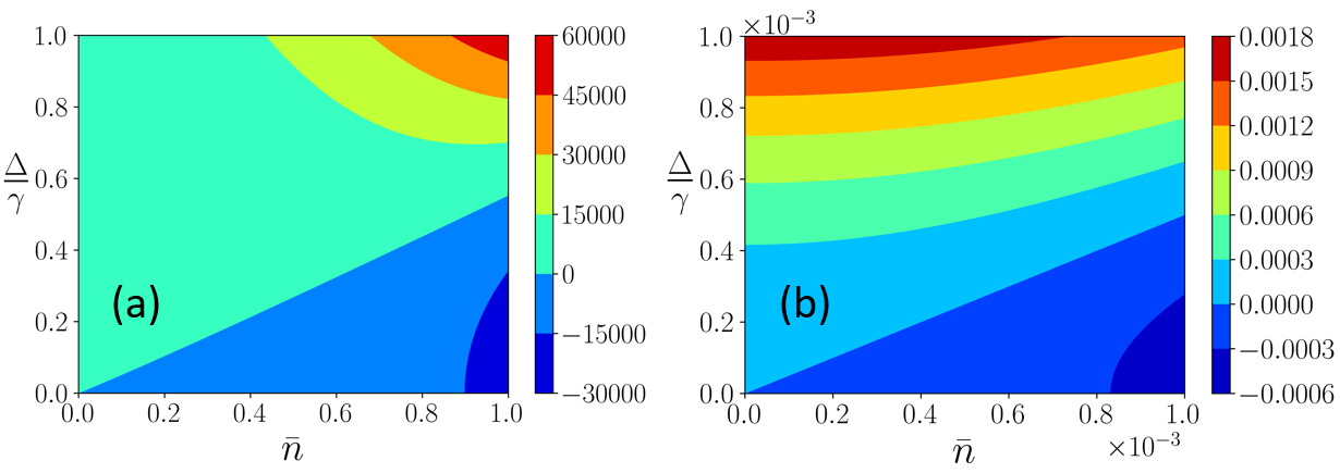
Figure 1: (a) Schematic diagram of the Λ\Lambda system with two ground states |g1⟩|g_{1}\rangle and |g2⟩\ket{g_{2}} and a single excited state |e⟩|e\rangle. (b) The discriminant DD as a function of the average photon number n¯\bar{n} and the reduced splitting Δ/γ\Delta/\gamma showing the different dynamical regimes of the incoherently driven Λ\Lambda-system. Regions of positive DD correspond to the underdamped regime; those of negative DD to the overdamped regime. (c) Coherence dynamics of the Λ\Lambda system initially in the fully mixed thermal state [ρgi​gi​(0)=1/2\rho_{g_{i}g_{i}}(0)=1/2, ρg1​g2​(0)=0\rho_{g_{1}g_{2}}(0)=0] for Δ/γ=10−2\Delta/\gamma=10^{-2}, γ=109\gamma=10^{9} s-1, n¯=10−3\bar{n}=10^{-3} and p=1p=1. Full line – numerically exact results, dashed line – analytical results. (d) Same as (c) for the initial coherent superposition [ρg1​g2​(0)=1/2\rho_{g_{1}g_{2}}(0)=1/2] with p=1p=1 (full line) and p=0p=0 (dashed line) for Δ/γ=2×10−2\Delta/\gamma=2\times 10^{-2} and n¯=10−3\bar{n}=10^{-3}.

To solve the BR equations (1) we recast them in matrix form x˙​(t)=Ax​(t)+d\dot{\textbf{x}}(t)=\textbf{A}\textbf{x}(t)+\textbf{d}, where x​(t)=(ρg1​g1,ρg1​g2R,ρg1​g2I)T\textbf{x}(t)=(\rho_{g_{1}g_{1}},\rho_{g_{1}g_{2}}^{R},\rho_{g_{1}g_{2}}^{I})^{T} is the state vector in the Liouville representation, 𝐀\mathbf{A} is the matrix of coefficients on the right-hand side of Eq. (1), d is a constant driving vector, and x0\textbf{x}_{0} defines the initial conditions for the density matrix SM. The solutions of the matrix BR equation x​(t)=eA​t​x0+∫0∞d​s​eA​(t−s)​d\textbf{x}(t)=e^{\textbf{A}t}\textbf{x}_{0}+\int_{0}^{\infty}dse^{\textbf{A}(t-s)}\textbf{d} may be expressed in terms of the eigenvalues of 𝐀\mathbf{A}, which determine the decay timescales of the different eigenmodes of the system SM. The general features of the solutions can be understood without finding the eigenvalues by considering the discriminant of the characteristic equation SM

D=B3+[C−32​A​(B+A2)]2D=B^{3}+[C-\frac{3}{2}A(B+A^{2})]^{2} (2)

where A=13​(5​r+2​γ)A=\frac{1}{3}(5r+2\gamma), B=13​[Δ2+r2+(2−p2)​r​(3​r+2​γ)]−A2B=\frac{1}{3}\big[\Delta^{2}+r^{2}+(2-p^{2})r(3r+2\gamma)\big]-A^{2}, and C=12​(3​r+2​γ)​[Δ2+(1−p2)​r2]+A3C=\frac{1}{2}(3r+2\gamma)\big[\Delta^{2}+(1-p^{2})r^{2}\big]+A^{3}. Three dynamical regimes can be distinguished depending on the sign of DD using the analogy with the damped harmonic oscillator Dodin et al. 2016a. In the underdamped regime (D>0)(D>0), 𝐀\mathbf{A} has one negative real and two complex conjugate eigenvalues, giving rise to an exponentially decaying and two oscillating eigenmodes. In the overdamped regime (D<0D<0) all of the eigenvalues are real and negative and thus the eigenmodes decay exponentially. In the critical regime (D=0D=0) all eigenvalues are real, negative, and at least two of them are equal.

As shown in the Supplementary Material SM, D=γ62916​∑k=06dk​(p,Δγ)​n¯kD=\frac{\gamma^{6}}{2916}\sum_{k=0}^{6}d_{k}(p,\frac{\Delta}{\gamma})\bar{n}^{k}. Figure 1(b) illustrates the different dynamical regimes of the incoherently driven Λ\Lambda-system obtained by solving the equation D=0D=0. We observe that the regions of positive DD are separated from those of negative DD by the critical line Δ/γ=f⁡(p)​n¯\Delta/\gamma=f(p)\bar{n}, where f⁡(p)f(p) is a universal function of pp SM, which gives the slope of the line. Thus, the overdamped regime is realized for Δ/γ<f⁡(p)​n¯\Delta/\gamma<f(p)\bar{n} and the underdamped regime for Δ/γ>f⁡(p)​n¯\Delta/\gamma>f(p)\bar{n}.

In the limit n¯→0\bar{n}\to 0 we obtain D=γ627​(Δγ)2​[(Δγ)2+4]2>0D=\frac{\gamma^{6}}{27}(\frac{\Delta}{\gamma})^{2}[(\frac{\Delta}{\gamma})^{2}+4]^{2}>0. Thus, as shown below, the Λ\Lambda-system predomonantly exhibits underdamped oscillatory dynamics under weak thermal driving, in marked contrast with the weakly driven V-system, where the underdamped regime is realized only for Δ/γ>1\Delta/\gamma>1 Tscherbul and Brumer 2014a; Dodin et al. 2016a; Koyu and Tscherbul 2018. This is because the ground states of the Λ\Lambda-system are not subject to spontaneous decay, unlike the excited states of the V-system. As a result, the two-photon coherence lifetime of the V-system scales as 1/γ1/\gamma, whereas that of the Λ\Lambda-system as 1/r1/r (as follows from Eq. (1) for p=0p=0). We note that while the overdamped regime does exist in the weakly driven Λ\Lambda-system when Δ/r<p2/2\Delta/r<p^{2}/2 SM, it is a highly restrictive condition, so we limit our discussion below to underdamped dynamics.

The eigenvalues λj\lambda_{j} of 𝐀\mathbf{A} give the decay rates of the corresponding eigenmodes SM

λj=−A+αj​B𝒯−βj​𝒯\lambda_{j}=-A+\alpha_{j}\frac{B}{\mathcal{T}}-\beta_{j}\mathcal{T} (3)

where 𝒯=E+D3\mathcal{T}=\sqrt[3]{E+\sqrt{D}}, E=[C−32​A​(B+A2)]E=[C-\frac{3}{2}A(B+A^{2})], ω=−1+i​32\omega=\frac{-1+i\sqrt{3}}{2}, and the quantities AA, BB, and CC are defined below Eq. (11) and αj\alpha_{j}, βj\beta_{j} are the cube roots of unity [(α1,β1)=(1,1)(\alpha_{1},\beta_{1})=(1,1), (α2,β2)=(ω2,ω)(\alpha_{2},\beta_{2})=(\omega^{2},\omega), and (α3,β3)=(ω,ω2)(\alpha_{3},\beta_{3})=(\omega,\omega^{2})]. We next consider the various limits of coherence dynamics defined by the sign of DD.

In the weakly driven regime (r/γ≪1r/\gamma\ll 1) the general expressions (32) can be simplified to give λ1=−(3​r+2​γ)=−2​γ\lambda_{1}=-(3r+2\gamma)=-2\gamma and λ2,3=−r​Q​(Δγ)±i​Δ\lambda_{2,3}=-rQ(\frac{\Delta}{\gamma})\pm i\Delta, where Q⁡(x)∈[1/2,1]Q(x)\in[1/2,1] is a smooth function, which increases monotonically with x=Δ/γx=\Delta/\gamma SM. The general analytical solutions of the BR equations in the underdamped regime may be written as (see the Supplementary Material SM for a derivation)

ρg1​g2R​(t)=[ρRg1​g2(0)cosΔt+ρIg1​g2(0)sinΔt)]e−r​Q​(Δγ)​t+p​r2​[4​γ2+Δ2]​[2​γ​e−2​γ​t−(2​γ​cos⁡Δ​t+Δ​sin⁡Δ​t)​e−r​Q​(Δγ)​t]\displaystyle\begin{split}\rho_{g_{1}g_{2}}^{R}(t)&=\big[\rho^{R}_{g_{1}g_{2}}(0)\cos\Delta t+\rho^{I}_{g_{1}g_{2}}(0)\sin\Delta t)\big]{e}^{-rQ(\frac{\Delta}{\gamma})t}\\ &+\frac{pr}{2[4\gamma^{2}+\Delta^{2}]}\bigg[2\gamma\text{e}^{-2\gamma t}-\left(2\gamma\cos\Delta t+\Delta\sin\Delta t\right){e}^{-rQ(\frac{\Delta}{\gamma})t}\bigg]\end{split}
ρg1​g2I​(t)=[−ρg1​g2R​(0)​sin⁡Δ​t+ρg1​g2I​(0)​cos⁡Δ​t]​e−r​Q​(Δγ)​t+p​r2​[4​γ2+Δ2]​[Δ​e−2​γ​t+(2​γ​sin⁡Δ​t−Δ​cos⁡Δ​t)​e−r​Q​(Δγ)​t].\displaystyle\begin{split}\rho_{g_{1}g_{2}}^{I}(t)&=\big[-\rho^{R}_{g_{1}g_{2}}(0)\sin\Delta t+\rho^{I}_{g_{1}g_{2}}(0)\cos\Delta t\big]\text{e}^{-rQ(\frac{\Delta}{\gamma})t}\\ &+\frac{pr}{2[4\gamma^{2}+\Delta^{2}]}\bigg[\Delta\text{e}^{-2\gamma t}+\left(2\gamma\sin\Delta t-\Delta\cos\Delta t\right)\text{e}^{-rQ(\frac{\Delta}{\gamma})t}\bigg].\end{split} (4)

Here, ρi​j​(0)\rho_{ij}(0) specify the initial conditions for the density matrix of the Λ\Lambda-system at t=0t=0, which we assume to be in an equal coherent superposition [ρg1​g1​(0)=ρg2​g2​(0)=1/2\rho_{g_{1}g_{1}}(0)=\rho_{g_{2}g_{2}}(0)=1/2].

In the important particular case of a fully mixed, coherence-free initial state, we have ρg1​g2​(0)=0\rho_{g_{1}g_{2}}(0)=0 and ρgi​gi​(0)=1/2\rho_{g_{i}g_{i}}(0)=1/2, and Eqs. (4) reduce to

ρg1​g2R​(t)\displaystyle\rho_{g_{1}g_{2}}^{R}(t) =p​r2​[4​γ2+Δ2]​[2​γ​e−2​γ​t−(2​γ​cos⁡Δ​t+Δ​sin⁡Δ​t)​e−r​Q​(Δγ)​t],\displaystyle=\frac{pr}{2[4\gamma^{2}+\Delta^{2}]}\big[2\gamma{e}^{-2\gamma t}-(2\gamma\cos\Delta t+\Delta\sin\Delta t){e}^{-rQ(\frac{\Delta}{\gamma})t}\big],
ρg1​g2I​(t)\displaystyle\rho_{g_{1}g_{2}}^{I}(t) =p​r2​[4​γ2+Δ2]​[Δ​e−2​γ​t+(2​γ​sin⁡Δ​t−Δ​cos⁡Δ​t)​e−r​Q​(ΔOPENγ)CLOSE].\displaystyle=\frac{pr}{2[4\gamma^{2}+\Delta^{2}]}[\Delta{e}^{-2\gamma t}+(2\gamma\sin\Delta t-\Delta\cos\Delta t){e}^{-rQ(\frac{\Delta}{\gamma)}}]. (5)

The concomitant population dynamics are given by

ρg1​g1​(t)=1(3​r+2​γ)​[r+γ+r2​e−2​γ​t].\rho_{g_{1}g_{1}}(t)=\frac{1}{(3r+2\gamma)}[r+\gamma+\frac{r}{2}{e}^{-2\gamma t}]. (6)

II.2 Noise-induced coherent dynamics of the Λ\Lambda-system

Figure 1(c) shows the ground-state population and coherence dynamics of the incoherently driven Λ\Lambda-system initially in the incoherent mixture of the ground states (ρgi​gi​(0)=1/2\rho_{g_{i}g_{i}}(0)=1/2) for p=1p=1 obtained by numerical solution of the BR equations. We observe that incoherent driving produces quantum beats due to Fano coherences in the absence of initial coherence in the system. The coherent oscillations decay on the timescale [r​Q​(Δγ)]−1\big[rQ(\frac{\Delta}{\gamma})\big]^{-1} in agreement with the analytical result (162). As the energy gap between the ground levels narrows down, the function Q⁡(Δγ)Q(\frac{\Delta}{\gamma}) decreases from 11 to 1/21/2 SM and the coherence lifetime increases by a factor of two. This is because the incoherent excitations |g⟩↔|ei⟩\ket{g}\leftrightarrow\ket{e_{i}} interfere more effectively at small Δ/γ\Delta/\gamma Koyu et al. 2021, as signaled by the non-negligible population-to-coherence coupling term −p​r1​r2​ρg1​g2R-p\sqrt{r_{1}r_{2}}\rho^{R}_{g_{1}g_{2}} in Eq. (1) in the limit Δ/γ≪1\Delta/\gamma\ll 1. We note that if incoherent driving is turned on gradually (rather than suddenly, as assumed here) the quantum beats will become suppressed, until they eventually disappear in the limit of adiabatically turned on incoherent driving Dodin et al. 2016b; Dodin and Brumer 2021b. However, steady-state Fano coherences generated by polarized incoherent excitation (see Sec. III) do survive the adiabatic turn-on Koyu et al. 2021.

If the Λ\Lambda-system is initialized in a coherent superposition of its ground states (ρg1​g2​(0)=1/2\rho_{g_{1}g_{2}}(0)=1/2) the dynamics under incoherent driving is given by Eq. (4) and contains additional terms proportional to ρg1​g2​(0)\rho_{g_{1}g_{2}}(0), which arise from the coherent initial condition SM. From Fig. 1(d) we observe that, in the absence of Fano interference (p=0p=0), the initially excited coherent superposition decays on the timescale 1/r1/r as expected due to incoherent transitions to the excited state |gi⟩→|e⟩|g_{i}\rangle\to|e\rangle followed by spontaneous decay to the vacuum modes of the electromagnetic field (indeed, the analytical solution of the BR equations (1) for p=0p=0 is ρg1​g2​(t)=ρg1​g2​(0)​e−(i​Δ+r)​t\rho_{g_{1}g_{2}}(t)=\rho_{g_{1}g_{2}}(0)e^{-(i\Delta+r)t}). Thus, Fano interference generated by incoherent driving “extends” the lifetime of the initial coherent superposition due to the noise-induced contribution (162).

We now turn to the overdamped dynamics of the strongly driven Λ\Lambda-system defined by the condition Δ/r<f⁡(n)\Delta/r<f(n). Expanding the eigenvalues of 𝐀\mathbf{A} in 1/n¯≪11/\bar{n}\ll 1 we find that λi\lambda_{i} do not depend on Δ/γ\Delta/\gamma for p<pcp<p_{c}, where pc≃1p_{c}\simeq 1 SM; Koyu and Tscherbul 2018. Remarkably, when the transition dipoles are nearly perfectly aligned (p>pcp>p_{c}), the scaling changes dramatically to λ2=−0.75​γn¯​(Δ/γ)2\lambda_{2}=-0.75\frac{\gamma}{\bar{n}}\left({\Delta}/{\gamma}\right)^{2}, giving rise to a coherent quasi-steady state with the lifetime τc=1.34​r/Δ2\tau_{c}=1.34{r}/{\Delta^{2}} that increases without limit as Δ→0\Delta\to 0. This point is illustrated in Figs. 2(a) and (b), where we plot the population and coherence dynamics of the Λ\Lambda-system strongly driven by incoherent light. We observe that the coherences rise quickly from zero to an intermediate “plateau” value, where they remain for t=τct=\tau_{c} before eventually decaying back to zero. Our analytical results for coherence dynamics are in excellent agreement with numerical calculations as shown in Figs. 2(a) and (b) (see the Supplementary Material SM). They reduce to prior Δ=0\Delta=0 results Ou et al. 2008 in the limit Δ→0\Delta\to 0, where the quasisteady states shown in Figs. 2(a) and (b) become true steady states.

Refer to caption
Figure 2: Ground-state population (a), coherence (b) and population difference (c) dynamics of the Λ\Lambda-system strongly driven by incoherent light (n¯=103\bar{n}=10^{3}, γ=109​s−1\gamma=10^{9}\kern 5.0pt\text{s}^{-1}, Δ/γ=10\Delta/\gamma=10 and p=1p=1). The Λ\Lambda system is initially in the fully mixed state ρ⁡(0)=12​(|g1⟩​⟨g1|+|g2⟩​⟨g2|)\rho(0)=\frac{1}{2}(|g_{1}\rangle\langle g_{1}|+|g_{2}\rangle\langle g_{2}|). (d) Time evolution of the von Neumann entropy with full Fano coherence [blue solid line] and without Fano coherence [red dashed line] for n¯=103\bar{n}=10^{3} and Δ/γ=102\Delta/\gamma=10^{2}. The ground states are initially in the coherent superposition ρ⁡(0)=12​(|g1⟩​⟨g1|+|g2⟩​⟨g2|+|g1⟩​⟨g2|+|g2⟩​⟨g1|)\rho(0)=\frac{1}{2}(|g_{1}\rangle\langle g_{1}|+|g_{2}\rangle\langle g_{2}|+|g_{1}\rangle\langle g_{2}|+|g_{2}\rangle\langle g_{1}|).

To understand the physical origin of long-lived Fano coherences in the Λ\Lambda-system, we use the effective decoherence rate model Koyu and Tscherbul 2018. As shown in Fig. 2(c) the decay of the ground-state population ρgi​gi\rho_{g_{i}g_{i}} is accompanied by a steady growth of the population inversion ρe​e−ρg1​g1\rho_{ee}-\rho_{g_{1}g_{1}}, which drives coherence generation. We observe that in the quasisteady state the time evolution of the population difference is identical to that of ρg1​g2R\rho_{g_{1}g_{2}}^{R} and that ρg1​g2I\rho^{I}_{g_{1}g_{2}} is time-independent. Neglecting the terms proportional to γ\gamma in Eq. (1), which is a good approximation in the strong pumping limit, and setting the left-land side of the resulting expression to zero, we obtain ρg1​g2I=−(Δ/r)​ρg1​g2R\rho_{g_{1}g_{2}}^{I}=-(\Delta/r)\rho^{R}_{g_{1}g_{2}} SM. This leads to a simplified equation of motion for ρg1​g2R{\rho}_{g_{1}g_{2}}^{R} valid at t>1/rt>1/r, ρ˙g1​g2R=−r⁡(1−p+Δ2/r2)​ρg1​g2R\dot{\rho}_{g_{1}g_{2}}^{R}=-r\left(1-p+{\Delta^{2}}/{r^{2}}\right)\rho_{g_{1}g_{2}}^{R}, which implies an exponential decay of the ground-state Fano coherence. The coherence lifetime

1/τdeff=r⁡(1−p+Δ2/r2),1/\tau_{d}^{\text{eff}}=r(1-p+{\Delta^{2}}/{r^{2}}), (7)

is consistent with the analytical result derived above. There are two distinct contributions to the overall decoherence rate in Eq. (170) which are similar to those identified in our previous work on the V-system Koyu and Tscherbul 2018: (i) the interplay between coherence-generating Fano interference and incoherent stimulated emission [the term r⁡(1−p)r(1-p)] and (ii) the coupling between the real and imaginary parts of the coherence due to the unitary evolution [the term Δ2/r\Delta^{2}/r]. The first mechanism does not contribute in the limit p→1p\to 1, explaining the formation of the long-lived coherent quasi-steady state shown in Fig. 2, which decays via mechanism (ii) at a rate ∝r/Δ2\propto r/\Delta^{2}.

Figure 2(d) shows the time evolution of the von Neumann entropy, 𝒮​(t)=−Tr​(ρ​ln​ρ)\mathcal{S}(t)=-\text{Tr}(\rho\text{ln}\rho), of the incoherently driven Λ\Lambda-system calculated with (p=1p=1) and without (p=0)(p=0) Fano coherence. The analytic expression for the entropy in terms of the populations and coherences is SM

𝒮⁡(t)=−[(ρg1​g1+|ρg1​g2|)​ln​(ρg1​g1+|ρg1​g2|)+(ρg1​g1−|ρg1​g2|)​ln​(ρg1​g1−|ρg1​g2|)+ρe​e​ln​ρe​e]\mathcal{S}(t)=-\Big[\big(\rho_{g_{1}g_{1}}+|\rho_{g_{1}g_{2}}|\big)\text{ln}\big(\rho_{g_{1}g_{1}}+|\rho_{g_{1}g_{2}}|\big)+\big(\rho_{g_{1}g_{1}}-|\rho_{g_{1}g_{2}}|\big)\text{ln}\big(\rho_{g_{1}g_{1}}-|\rho_{g_{1}g_{2}}|\big)+\rho_{ee}\text{ln}\rho_{ee}\Big] (8)

with ρe​e=1−ρg1​g1−ρg2​g2\rho_{ee}=1-\rho_{g_{1}g_{1}}-\rho_{g_{2}g_{2}}. We observe that the entropy of the long-lived coherent quasi-steady state is two times smaller than that of the corresponding p=0p=0 thermal state due to the presence of substantial coherences in the energy basis. The low-entropy state persists for τc∝(r/Δ2)\tau_{c}\propto(r/\Delta^{2}) before decaying to the high-entropy thermal state.

Refer to caption
Figure 3: (a) Schematic diagram of the Λ\Lambda-system configuration to detect Fano coherences in He* atoms. The Sm=±13↔P03{}^{3}S_{m=\pm 1}\leftrightarrow{{}^{3}}P_{0} transitions are indicated by double-headed arrows. The magnetic field is parallel to the propagation vector of the xx-polarized incoherent light, which defines the quantization axis. (b) Ground-state coherence dynamics of He* excited by xx-polarized incoherent light with the parameters γ=108\gamma=10^{8} s-1, n¯=10−3\bar{n}=10^{-3}, and Δ/γ=10−2\Delta/\gamma=10^{-2}.

III Proposal for experimental observation of Fano coherences in He∗ atoms

We finally turn to the question of experimental observation of Fano coherences. We suggest metastable He(23​S12^{3}S_{1}) atoms Vassen et al. 2012; Vassen et al. 2016 as a readily realizable Λ\Lambda-system, in which to observe noise-induced coherent dynamics. The Λ\Lambda-system is formed by the m=±1m=\pm 1 Zeeman sublevels of the metastable S3{}^{3}S state and the nondegenerate excited P03{}^{3}P_{0} state as shown in Fig. 3(a). The energy gap Δ\Delta between the Zeeman sublevels is continuously tunable with an external magnetic field, providing access to both the overdamped and underdamped regimes of coherence dynamics. The Sm=±13↔P03{}^{3}S_{m=\pm 1}\leftrightarrow{{}^{3}}P_{0} transitions are driven by a spectrally broadened laser field polarized in the xx-direction. This excitation scheme allows us to (i) neglect radiative transitions involving the m=0m=0 ground-state Zeeman sublevel, thereby realizing an ideal three-level Λ\Lambda-system (since He∗ has no hyperfine structure), and (ii) bypass the p=1p=1 condition needed to generate Fano interference via isotropic incoherent excitation Dodin et al. 2018; Koyu et al. 2021. Because both of the Λ\Lambda-system transitions couple to the same polarization mode of the incoherent radiation field, the BR equations (1) can be simplified by replacing r+γ→γr+\gamma\to\gamma Dodin et al. 2018; Koyu et al. 2021; SM.

Figure 3(b) shows ground-state Fano coherence dynamics of a He∗ atom driven by xx-polarized incoherent light starting from a coherence-free initial state ρgi​gi​(0)=1/2\rho_{g_{i}g_{i}}(0)=1/2. As in the case of isotropic incoherent excitation considered above, the coherences exhibit quantum beats with frequency Δ\Delta and lifetime 1/(Q​r)1/(Qr). The coherent evolution could be probed by applying a π/2\pi/2 radiofrequency pulse (as part of the standard Ramsey sequence Degen et al. 2017; Vassen et al. 2016) to convert the coherences to the populations of the m=±1m=\pm 1 atomic states, which could be measured by, e.g., state-selective photoionization Vassen et al. 2012; Vassen et al. 2016.

Significantly, as shown in Fig. 3(b), the Fano coherences generated by polarized incoherent excitation do not vanish in the steady state (t→∞)(t\to\infty) unlike those in isotropic excitation. This is a result of the imbalance between polarized incoherent excitation and spontaneous emission (the former is directional whereas the latter is isotropic), leading to a breakdown of detailed balance, and the emergence of non-equilibrium steady-states Agarwal and Menon 2001; Dodin et al. 2018; Koyu et al. 2021. The steady-state populations and coherences SM

ρgi​gi(SS)\displaystyle\rho_{g_{i}g_{i}}^{(\text{SS})} =(r+γ)​Δ2+r2​γ(3​r+2​γ)​Δ2+2​r2​γ,\displaystyle=\frac{(r+\gamma)\Delta^{2}+r^{2}\gamma}{(3r+2\gamma)\Delta^{2}+2r^{2}\gamma},
ρg1​g2R⁡(SS)=−r2​γ(3​r+2​γ)​Δ2+2​r2​γ\displaystyle\begin{split}\rho_{g_{1}g_{2}}^{R(\text{SS})}&=-\frac{r^{2}\gamma}{(3r+2\gamma)\Delta^{2}+2r^{2}\gamma}\end{split} (9)

deviate from the values expected in thermal equilibrium [ρgi​gi(SS,th)=(r+γ)/(3r+2γ)][\rho_{g_{i}g_{i}}^{(\text{SS,th})}=(r+\gamma)/(3r+2\gamma)]. As in the case of the V-system Koyu et al. 2021, this could be used to detect Fano coherences by measuring the deviation of steady-state populations from their expected values in thermodynamic equilibrium.

IV Summary

We have explored the quantum dynamics of noise-induced Fano coherences in a prototypical three-level Λ\Lambda-system driven by BBR. In contrast to its V-system counterpart Tscherbul and Brumer 2014a; Dodin et al. 2016a; Dodin et al. 2018; Koyu and Tscherbul 2018 the weakly driven Λ\Lambda-system almost always remains in the underdamped regime characterized by oscillatory coherence dynamics that decays on the timescale 1/r1/r (for OPENΔ/γ≫1)\Delta/\gamma\gg 1) or 2/r2/r (for OPENΔ/γ≪1)\Delta/\gamma\ll 1), which can be extremely long for small pumping rates r/γ≃10−9r/\gamma\simeq 10^{-9} relevant for photosynthetic solar light harvesting Hoki and Brumer 2011; Tscherbul and Brumer 2014a. This also suggests that Fano coherences may find applications in, e.g., quantum sensing Degen et al. 2017, where a qubit’s coherence time is a key figure of merit. Similarly, the long-lived coherent quasi-steady states that arise in the strongly driven Λ\Lambda-system [see Fig. (2)] have lower entropy than the corresponding thermal states, motivating further research into the origin and potential utility of these states [as well as the true coherent steady states shown in Fig. 3(b)] in multilevel quantum systems.

While both the V- and Λ\Lambda systems are three-level systems, the crucial difference between them is that the nearly degenerate levels of the V-system are subject to spontaneous emission, whereas those of the Λ\Lambda system are not. As a consequence, these systems exhibit very different noise-driven dynamics in the regime, where spontaneous emission rate is much higher than the incoherent driving rate. This occurs in the weakly driven regime (r/γ≪1)(r/\gamma\ll 1) of importance for photosynthetic light-harvesting under ambient sunlight conditions. On the other hand, if the rate of spontaneous emission is smaller than that of incoherent pumping (the strongly driven regime, r/γ≫1r/\gamma\gg 1), then one might expect the V and Λ\Lambda systems to display similar dynamical features, as is indeed the case. One notable example is provided by the long-lived coherent quasi-steady states, which have exactly the same lifetimes for both the V and Λ\Lambda systems, and can be described by the same effective decoherence rate model Koyu and Tscherbul 2018.

In addition to similar dynamical behavior, the mathematical features of both models in the strongly driven regime are fairly similar. For instance, the zero-discriminant equation of the strongly driven Λ\Lambda-system given by Eq. (21) of the Supplementary Material SM is the same as that of the V-system. Furthermore, the expressions for the population and coherence dynamics of the strongly driven Λ\Lambda- and V-systems have the same form when expressed in terms of the coefficients Ai,BiA_{i},B_{i}, and CiC_{i} (see SM, Sec. I.E2). Nevertheless, these coefficients have a completely different dependence on the transition dipole alignment factor pp for the V and Λ−\Lambda-systems.

Finally, we propose an experimental scenario for detecting Fano coherences by driving circularly polarized Sm=±13↔P03{}^{3}S_{m=\pm 1}\leftrightarrow{{}^{3}}P_{0} transitions in metastable He atoms excited by xx-polarized incoherent radiation and subject to an external magnetic field. Our results suggest that thermal driving can lead to novel long-lived quantum beats and non-thermal coherent steady states in multilevel atomic and molecular systems, motivating further studies of Fano coherences in more complex multilevel molecular systems and of their role in photosynthetic energy transfer processes and in quantum information science.

Supplementary Material

The Supplementary Material contains a detailed derivation of the analytical solutions of the BR equations presented in the main text.

Acknowledgements

We thank Prof. Amar Vutha for suggesting He∗ as an experimental realization of the Λ\Lambda-system, and Prof. Paul Brumer for a valuable discussion. This work was partially supported by NSF PHY-1912668.

References

  • Brumer (2018) P. Brumer, Shedding (incoherent) light on quantum effects in light-induced biological processes, J. Phys. Chem. Lett. 9, 2946 (2018).
  • Cao et al. (2020) J. Cao, R. J. Cogdell, D. F. Coker, H.-G. Duan, J. Hauer, U. Kleinekathöfer, T. L. C. Jansen, T. Mančal, R. J. D. Miller, J. P. Ogilvie, V. I. Prokhorenko, T. Renger, H.-S. Tan, R. Tempelaar, M. Thorwart, E. Thyrhaug, S. Westenhoff, and D. Zigmantas, Quantum biology revisited, Science Advances 6, eaaz4888 (2020).
  • Dodin and Brumer (2021a) A. Dodin and P. Brumer, Noise-induced coherence in molecular processes, J. Phys. B 54, 223001 (2021a).
  • Tscherbul and Brumer (2014a) T. V. Tscherbul and P. Brumer, Long-lived quasistationary coherences in a VV-type system driven by incoherent light, Phys. Rev. Lett. 113, 113601 (2014a).
  • Olšina et al. (2014) J. Olšina, A. G. Dijkstra, C. Wang, and J. Cao, Can natural sunlight induce coherent exciton dynamics?, arXiv:1408.5385 (2014).
  • Kosloff and Levy (2014) R. Kosloff and A. Levy, Quantum heat engines and refrigerators: Continuous devices, Annu. Rev. Phys. Chem. 65, 365 (2014).
  • Scully et al. (2011) M. O. Scully, K. R. Chapin, K. E. Dorfman, M. B. Kim, and A. Svidzinsky, Quantum heat engine power can be increased by noise-induced coherence, Proc. Natl. Acad. Sci. USA 108, 15097 (2011).
  • Dorfman et al. (2013) K. E. Dorfman, D. V. Voronine, S. Mukamel, and M. O. Scully, Photosynthetic reaction center as a quantum heat engine, Proc. Natl. Acad. Sci. USA 110, 2746 (2013).
  • Beloy et al. (2006) K. Beloy, U. I. Safronova, and A. Derevianko, High-accuracy calculation of the blackbody radiation shift in the Cs133{}^{133}\mathrm{Cs} primary frequency standard, Phys. Rev. Lett. 97, 040801 (2006).
  • Safronova et al. (2012) M. S. Safronova, M. G. Kozlov, and C. W. Clark, Blackbody radiation shifts in optical atomic clocks, IEEE Transactions on Ultrasonics, Ferroelectrics, and Frequency Control 59, 439 (2012).
  • Ovsiannikov et al. (2011) V. D. Ovsiannikov, A. Derevianko, and K. Gibble, Rydberg spectroscopy in an optical lattice: Blackbody thermometry for atomic clocks, Phys. Rev. Lett. 107, 093003 (2011).
  • Lisdat et al. (2021) C. Lisdat, S. Dörscher, I. Nosske, and U. Sterr, Blackbody radiation shift in strontium lattice clocks revisited, Phys. Rev. Research 3, L042036 (2021).
  • Kassal et al. (2013) I. Kassal, J. Yuen-Zhou, and S. Rahimi-Keshari, Does coherence enhance transport in photosynthesis?, J. Phys. Chem. Lett. 4, 362 (2013).
  • León-Montiel et al. (2014) R. d. J. León-Montiel, I. Kassal, and J. P. Torres, Importance of excitation and trapping conditions in photosynthetic environment-assisted energy transport, J. Phys. Chem. B 118, 10588 (2014).
  • Tscherbul and Brumer (2018) T. V. Tscherbul and P. Brumer, Non-equilibrium stationary coherences in photosynthetic energy transfer under weak-field incoherent illumination, J. Chem. Phys. 148, 124114 (2018).
  • Yang and Cao (2020) P.-Y. Yang and J. Cao, Steady-state analysis of light-harvesting energy transfer driven by incoherent light: From dimers to networks, J. Phys. Chem. Lett. 11, 7204 (2020).
  • Chuang and Brumer (2020) C. Chuang and P. Brumer, LH1-RC light-harvesting photocycle under realistic light–matter conditions, J. Chem. Phys. 152, 154101 (2020).
  • Polli et al. (2010) D. Polli, P. Altoè, O. Weingart, K. M. Spillane, C. Manzoni, D. Brida, G. Tomasello, G. Orlandi, P. Kukura, R. A. Mathies, M. Garavelli, and G. Cerullo, Conical intersection dynamics of the primary photoisomerization event in vision, Nature 467, 440 (2010).
  • Schulten and Hayashi (2014) K. Schulten and S. Hayashi, Quantum biology of retinal, in Quantum Effects in Biology, edited by G. S. Engel, M. B. Plenio, M. Mohseni, and Y. Omar (Cambridge University Press, Cambridge, 2014) pp. 237–263.
  • Tscherbul and Brumer (2014b) T. V. Tscherbul and P. Brumer, Excitation of biomolecules with incoherent light: Quantum yield for the photoisomerization of model retinal, J. Phys. Chem. A 118, 3100 (2014b).
  • Tscherbul and Brumer (2015a) T. V. Tscherbul and P. Brumer, Quantum coherence effects in natural light-induced processes: cis–trans photoisomerization of model retinal under incoherent excitation, Phys. Chem. Chem. Phys. 17, 30904 (2015a).
  • Chuang and Brumer (2022) C. Chuang and P. Brumer, Steady state photoisomerization quantum yield of model rhodopsin: Insights from wavepacket dynamics?, J. Phys. Chem. Lett. 13, 4963 (2022).
  • Cohen-Tannoudji et al. (2004) C. Cohen-Tannoudji, J. Dupont-Roc, and G. Grynberg, Atom-Photon Interactions: Basic Processes and Applications (Wiley-VCH, 2004).
  • Blum (2011) K. Blum, Density Matrix Theory and Applications, Chap. 8 (Springer, 2011).
  • Wilhelm et al. (2007) F. K. Wilhelm, M. J. Storcz, U. Hartmann, and M. R. Geller, Superconducting qubits ii: Decoherence, in Manipulating Quantum Coherence in Solid State Systems, edited by M. E. Flatté and I. Ţifrea (Springer Netherlands, Dordrecht, 2007) pp. 195–232.
  • Jeske et al. (2015) J. Jeske, D. J. Ing, M. B. Plenio, S. F. Huelga, and J. H. Cole, Bloch-Redfield equations for modeling light-harvesting complexes, J. Chem. Phys. 142, 064104 (2015).
  • Dodin et al. (2016a) A. Dodin, T. V. Tscherbul, and P. Brumer, Quantum dynamics of incoherently driven V-type systems: Analytic solutions beyond the secular approximation, J. Chem. Phys. 144, 244108 (2016a).
  • Dodin et al. (2018) A. Dodin, T. V. Tscherbul, R. Alicki, A. Vutha, and P. Brumer, Secular versus nonsecular Redfield dynamics and Fano coherences in incoherent excitation: An experimental proposal, Phys. Rev. A 97, 013421 (2018).
  • Koyu and Tscherbul (2018) S. Koyu and T. V. Tscherbul, Long-lived quantum coherences in a 𝖵\mathsf{V}-type system strongly driven by a thermal environment, Phys. Rev. A 98, 023811 (2018).
  • Tscherbul and Brumer (2015b) T. V. Tscherbul and P. Brumer, Partial secular Bloch-Redfield master equation for incoherent excitation of multilevel quantum systems, J. Chem. Phys. 142, 104107 (2015b).
  • Eastham et al. (2016) P. R. Eastham, P. Kirton, H. M. Cammack, B. W. Lovett, and J. Keeling, Bath-induced coherence and the secular approximation, Phys. Rev. A 94, 012110 (2016).
  • Wang et al. (2019) Z. Wang, W. Wu, and J. Wang, Steady-state entanglement and coherence of two coupled qubits in equilibrium and nonequilibrium environments, Phys. Rev. A 99, 042320 (2019).
  • Liao and Liang (2021) C.-Y. Liao and X.-T. Liang, The Lindblad and Redfield forms derived from the Born–Markov master equation without secular approximation and their applications, Comm. Theor. Phys. 73, 095101 (2021).
  • Merkli et al. (2015) M. Merkli, H. Song, and G. P. Berman, Multiscale dynamics of open three-level quantum systems with two quasi-degenerate levels, J. Phys. A 48, 275304 (2015).
  • Trushechkin (2021) A. Trushechkin, Unified Gorini-Kossakowski-Lindblad-Sudarshan quantum master equation beyond the secular approximation, Phys. Rev. A 103, 062226 (2021).
  • Fleischhauer et al. (1992) M. Fleischhauer, C. H. Keitel, M. O. Scully, and C. Su, Lasing without inversion and enhancement of the index of refraction via interference of incoherent pump processes, Opt. Commun. 87, 109 (1992).
  • Hegerfeldt and Plenio (1993) G. C. Hegerfeldt and M. B. Plenio, Coherence with incoherent light: A new type of quantum beat for a single atom, Phys. Rev. A 47, 2186 (1993).
  • Kozlov et al. (2006) V. V. Kozlov, Y. Rostovtsev, and M. O. Scully, Inducing quantum coherence via decays and incoherent pumping with application to population trapping, lasing without inversion, and quenching of spontaneous emission, Phys. Rev. A 74, 063829 (2006).
  • Ou et al. (2008) B.-Q. Ou, L.-M. Liang, and C.-Z. Li, Coherence induced by incoherent pumping field and decay process in three-level Λ\Lambda-type atomic system, Opt. Commun. 281, 4940 (2008).
  • Koyu et al. (2021) S. Koyu, A. Dodin, P. Brumer, and T. V. Tscherbul, Steady-state Fano coherences in a V-type system driven by polarized incoherent light, Phys. Rev. Research 3, 013295 (2021).
  • Ficek and Swain (2005) Z. Ficek and S. Swain, Quantum Interference and Coherence: Theory and Experiments (Springer-Verlag, New York, 2005).
  • Patnaik and Agarwal (1999) A. K. Patnaik and G. S. Agarwal, Cavity-induced coherence effects in spontaneous emissions from preselection of polarization, Phys. Rev. A 59, 3015 (1999).
  • Kapale et al. (2003) K. T. Kapale, M. O. Scully, S.-Y. Zhu, and M. S. Zubairy, Quenching of spontaneous emission through interference of incoherent pump processes, Phys. Rev. A 67, 023804 (2003).
  • Jung and Brumer (2020) K. A. Jung and P. Brumer, Energy transfer under natural incoherent light: Effects of asymmetry on efficiency, J. Chem. Phys. 153, 114102 (2020).
  • Janković and Mančal (2020) V. Janković and T. Mančal, Nonequilibrium steady-state picture of incoherent light-induced excitation harvesting, J. Chem. Phys. 153, 244110 (2020).
  • Tomasi et al. (2021) S. Tomasi, D. M. Rouse, E. M. Gauger, B. W. Lovett, and I. Kassal, Environmentally improved coherent light harvesting, J. Phys. Chem. Lett. 12, 6143 (2021).
  • Latune et al. (2020) C. L. Latune, I. Sinayskiy, and F. Petruccione, Negative contributions to entropy production induced by quantum coherences, Phys. Rev. A 102, 042220 (2020).
  • Agarwal and Menon (2001) G. S. Agarwal and S. Menon, Quantum interferences and the question of thermodynamic equilibrium, Phys. Rev. A 63, 023818 (2001).
  • Han et al. (2021) H. S. Han, A. Lee, K. Sinha, F. K. Fatemi, and S. L. Rolston, Observation of vacuum-induced collective quantum beats, Phys. Rev. Lett. 127, 073604 (2021).
  • Fleischhauer et al. (2005) M. Fleischhauer, A. Imamoglu, and J. P. Marangos, Electromagnetically induced transparency: Optics in coherent media, Rev. Mod. Phys. 77, 633 (2005).
  • Altenmüller (1995) T. P. Altenmüller, Are there quantum beats from vacuum-induced coherence?, Z. Phys. D 34, 157 (1995).
  • Hoki and Brumer (2011) K. Hoki and P. Brumer, Excitation of biomolecules by coherent vs. incoherent light: Model rhodopsin photoisomerization, Procedia Chem. 3, 122 (2011).
  • Breuer and Petruccione (2006) H.-P. Breuer and F. Petruccione, The Theory of Open Quantum Systems (Clarendon Press, Oxford, 2006).
  • McCauley et al. (2020) G. McCauley, B. Cruikshank, D. I. Bondar, and K. Jacobs, Accurate Lindblad-form master equation for weakly damped quantum systems across all regimes, npj Quantum Information 6, 74 (2020).
  • (55) See Supplementary Material at [URL] for a derivation of analytical solutions of the BR equations.
  • Dodin et al. (2016b) A. Dodin, T. V. Tscherbul, and P. Brumer, Coherent dynamics of v-type systems driven by time-dependent incoherent radiation, J. Chem. Phys. 145, 244313 (2016b).
  • Dodin and Brumer (2021b) A. Dodin and P. Brumer, Generalized adiabatic theorems: Quantum systems driven by modulated time-varying fields, PRX Quantum 2, 030302 (2021b).
  • Vassen et al. (2012) W. Vassen, C. Cohen-Tannoudji, M. Leduc, D. Boiron, C. I. Westbrook, A. Truscott, K. Baldwin, G. Birkl, P. Cancio, and M. Trippenbach, Cold and trapped metastable noble gases, Rev. Mod. Phys. 84, 175 (2012).
  • Vassen et al. (2016) W. Vassen, R. P. M. J. W. Notermans, R. J. Rengelink, and R. F. H. J. van der Beek, Ultracold metastable helium: Ramsey fringes and atom interferometry, Appl. Phys. B 122, 289 (2016).
  • Degen et al. (2017) C. L. Degen, F. Reinhard, and P. Cappellaro, Quantum sensing, Rev. Mod. Phys. 89, 035002 (2017).

Supplemental Material

This Supplementary Material presents a derivation of analytical solutions of the Bloch-Redfield (BR) quantum master equations for the Λ\Lambda-system driven by isotropic incoherent light (Sec. I). In Sec. II we derive and solve the BR equations for the Λ\Lambda-system driven by xx-polarized incoherent light.

Within Sec. I, section IA provides an overview of the BR equations and of the theoretical procedures used to obtain their analytical solutions. The dynamical regimes of the Λ\Lambda-system are classified in Sec. IB. In Secs. IC and ID we derive the expressions for the eigenvalues and eigenvectors of the coefficient matrix 𝐀\mathbf{A} (see main text). Section IE is devoted to the derivation of analytical solutions to the BR-equations in both the overdamped and the underdamped regimes of the strong pumping limit. The effective decoherence rate model used to explain the physical origin of long-lived Fano coherences is derived in Sec. IF.

Section IG is devoted to the weak pumping limit. We derive the eigenvalues of matrix 𝐀\mathbf{A}, discuss their qualitative features, and provide analytical solutions for the population and coherence dynamics. In Sec. IH, we describe the procedure of computing von Neumann entropy of the incoherently driven Λ\Lambda-system.

Section IIA presents the derivation of the BR equations for the Λ\Lambda-system driven by polarized incoherent radiation. The steady-state solutions of these equations are discussed in Sec. IIB. The coefficients relevant to the analytical solutions of the BR equations are listed in Sec. III.

I Λ\Lambda-system driven by incoherent light: The Bloch-Redfield equations and their analytical solution

I.1 Bloch-Redfield equations and their general solutions

We consider a symmetric Λ\Lambda-system (see main text and Fig. 1) that interacts with a suddenly turned on incoherent radiation field. Within the framework of the Born-Markov approximation, the time dynamics of a Λ\Lambda-system is given by the Bloch-Redfield (BR) quantum master equations Tscherbul and Brumer 2015b

ρ˙gi​gi\displaystyle\dot{\rho}_{g_{i}g_{i}} =−ri​ρgi​gi+(ri+γi)​ρe​e−p​r1​r2​ρg1​g2R\displaystyle=-r_{i}\rho_{g_{i}g_{i}}+(r_{i}+\gamma_{i})\rho_{ee}-p\sqrt{r_{1}r_{2}}\rho^{R}_{g_{1}g_{2}} (1)
ρ˙g1​g2=−12​(r1+r2)​ρg1​g2−i​ρg1​g2​Δ+p⁡(r1​r2+γ1​γ2)​ρe​e−p2​r1​r2​(ρg1​g1+ρg2​g2)\displaystyle\begin{split}\dot{\rho}_{g_{1}g_{2}}&=-\frac{1}{2}(r_{1}+r_{2})\rho_{g_{1}g_{2}}-i\rho_{g_{1}g_{2}}\Delta+p(\sqrt{r_{1}r_{2}}+\sqrt{\gamma_{1}\gamma_{2}})\rho_{ee}-\frac{p}{2}\sqrt{r_{1}r_{2}}(\rho_{g_{1}g_{1}}+\rho_{g_{2}g_{2}})\end{split} (2)

where

ρg1​g2=ρg1​g2R+i​ρg1​g2I\rho_{g_{1}g_{2}}=\rho^{R}_{g_{1}g_{2}}+i\rho^{I}_{g_{1}g_{2}} (3)

is the coherence between the ground states |g1⟩\ket{g_{1}} and |g2⟩\ket{g_{2}} with the real and imaginary parts ρg1​g2R\rho^{R}_{g_{1}g_{2}} and ρg1​g2I\rho^{I}_{g_{1}g_{2}}, γi\gamma_{i} is the radiative decay rate of level |gi⟩\ket{g_{i}} (i=1,2i=1,2), ri=n¯​γir_{i}=\bar{n}\gamma_{i} is the incoherent pumping rate, p=(𝝁g1​e⋅𝝁g2​e)/μg1​e​μg2​ep=(\bm{\mu}_{g_{1}e}\cdot\bm{\mu}_{g_{2}e})/\mu_{g_{1}e}\mu_{g_{2}e} is the transition dipole alignment factor, and 𝝁g1​e\bm{\mu}_{g_{1}e}, 𝝁g2​e\bm{\mu}_{g_{2}e} are the matrix elements of the transition dipole moment vector between the excited and ground states |e⟩\ket{e} and |gi⟩\ket{g_{i}}.

Figure 1: Schematic diagram of the Λ\Lambda-system with two quasi-degenerate ground states |g1⟩|g_{1}\rangle and |g2⟩|g_{2}\rangle and a single excited state |e⟩|e\rangle. The incoherent pumping rates are rr, the spontaneous decay rate of the excited state is γ\gamma, and the energy gap between the ground states is Δ\Delta.

For a symmetric Λ\Lambda-system, where r1=r2=rr_{1}=r_{2}=r, and γ1=γ2=γ\gamma_{1}=\gamma_{2}=\gamma, the BR equations (1) - (2) combined with Eq. (3) reduce to

ρ˙g1​g1\displaystyle\dot{\rho}_{g_{1}g_{1}} =−r​ρg1​g1+(r+γ)​ρe​e−p​r​ρg1​g2R\displaystyle=-r\rho_{g_{1}g_{1}}+(r+\gamma)\rho_{ee}-pr\rho^{R}_{g_{1}g_{2}} (4)
ρ˙g1​g2R\displaystyle\dot{\rho}^{R}_{g_{1}g_{2}} =−p​r​ρg1​g1+p⁡(r+γ)​ρe​e−r​ρg1​g2R+Δ​ρg1​g2I\displaystyle=-pr\rho_{g_{1}g_{1}}+p(r+\gamma)\rho_{ee}-r\rho^{R}_{g_{1}g_{2}}+\Delta\rho^{I}_{g_{1}g_{2}} (5)
ρ˙g1​g2I\displaystyle\dot{\rho}^{I}_{g_{1}g_{2}} =−Δ​ρg1​g2R−r​ρg1​g2I\displaystyle=-\Delta\rho^{R}_{g_{1}g_{2}}-r\rho^{I}_{g_{1}g_{2}} (6)

These equations can be expressed in matrix form

[ρ˙g1​g1ρ˙g1​g2Rρ˙g1​g2I]=[−(3​r+2​γ)−p​r0−p⁡(3​r+2​γ)−rΔ0−Δ−r]​[ρg1​g1ρg1​g2Rρg1​g2I]+[(r+γ)p⁡(r+γ)0]\begin{bmatrix}\dot{\rho}_{g_{1}g_{1}}\\ \dot{\rho}^{R}_{g_{1}g_{2}}\\ \dot{\rho}^{I}_{g_{1}g_{2}}\\ \end{bmatrix}=\begin{bmatrix}-(3r+2\gamma)&-pr&0\\ -p(3r+2\gamma)&-r&\Delta\\ 0&-\Delta&-r\\ \end{bmatrix}\begin{bmatrix}\rho_{g_{1}g_{1}}\\ \rho^{R}_{g_{1}g_{2}}\\ \rho^{I}_{g_{1}g_{2}}\\ \end{bmatrix}+\begin{bmatrix}(r+\gamma)\\ p(r+\gamma)\\ 0\\ \end{bmatrix} (7)

or

x˙​(t)=Ax​(t)+d\dot{\textbf{x}}(t)=\textbf{A}\textbf{x}(t)+\textbf{d} (8)

where x​(t)=[ρg1​g1ρg1​g2Rρg1​g2I]T\textbf{x}(t)=\begin{bmatrix}\rho_{g_{1}g_{1}}&\rho_{g_{1}g_{2}}^{R}&\rho_{g_{1}g_{2}}^{I}\end{bmatrix}^{T} is the state vector in the Liouville representation,

A=[−(3​r+2​γ)−p​r0−p⁡(3​r+2​γ)−rΔ0−Δ−r]\textbf{A}=\begin{bmatrix}-(3r+2\gamma)&-pr&0\\ -p(3r+2\gamma)&-r&\Delta\\ 0&-\Delta&-r\\ \end{bmatrix} (9)

is the matrix of coefficients on the right-hand side of Eqs. (4)-(6), and d=[(r+γ)p⁡(r+γ)0]T\textbf{d}=\begin{bmatrix}(r+\gamma)&p(r+\gamma)&0\end{bmatrix}^{T} is the driving vector.

The inhomogeneous differential equations (8) can be explicitly solved as

x​(t)=eA​t​x0+∫0td​s​eA​(t−s)​d,{\textbf{x}}(t)=e^{\textbf{A}t}\textbf{x}_{0}+\int_{0}^{t}dse^{\textbf{A}(t-s)}\textbf{d}, (10)

where x0\textbf{x}_{0} defines the initial conditions for the density matrix. Since we are interested in the generation of noise-induced coherences by incoherent driving, we choose an equal incoherent mixture of the ground states as our initial state, i.e., ρg1​g1​(t)=ρg2​g2​(t)=12\rho_{g_{1}g_{1}}(t)=\rho_{g_{2}g_{2}}(t)=\frac{1}{2} or x0=[12,0,0]T\textbf{x}_{0}=[\frac{1}{2},0,0]^{T}.

I.2 Dynamical regimes

The physical behavior of the Λ\Lambda-system as described by the BR equations (8) is governed by the eigenvalues of the coefficient matrix A. Without explicitly finding the eigenvalues, their general features can be understood by analyzing the discriminant DD of the characteristic equation for A

D=B3+[C−32​A​(B+A2)]2D=B^{3}+\Big[C-\frac{3}{2}A(B+A^{2})\Big]^{2} (11)

where,

A\displaystyle A =13​(5​r+2​γ)\displaystyle=\frac{1}{3}(5r+2\gamma) (12)
B\displaystyle B =13​[Δ2+r2+(2−p2)​r​(3​r+2​γ)]−A2\displaystyle=\frac{1}{3}\big[\Delta^{2}+r^{2}+(2-p^{2})r(3r+2\gamma)\big]-A^{2} (13)
C\displaystyle C =12​(3​r+2​γ)​[Δ2+(1−p2)​r2]+A3\displaystyle=\frac{1}{2}(3r+2\gamma)\big[\Delta^{2}+(1-p^{2})r^{2}\big]+A^{3} (14)

The dynamical regimes of a Λ\Lambda-system can be classified into three types depending on the sign of DD:

  1. 1.

    Underdamped regime (D>0D>0) The coefficient matrix A given by Eq. (9) has three roots, with one of them being real and the other two being complex conjugates of each other. The normal modes consist of an exponentially decaying eigenmode and two oscillating eigenmodes.

  2. 2.

    Overdamped regime (D<0D<0) The roots of the coefficient matrix A are all real and negative. The normal modes all decay exponentially as a function of time.

  3. 3.

    Critical regime (D=0D=0) The coefficient matrix A has three real roots with at least two of them being equal. This regime is at the boundary between the underdamped and overdamped regimes.

It is convenient to express the terms AA, BB, CC as a function of the occupation number n¯=r/γ\bar{n}=r/\gamma

A\displaystyle A =γ3​(5​n¯+2),\displaystyle=\frac{\gamma}{3}\big(5\bar{n}+2\big), (15)
B\displaystyle B =γ29​[(3​Δ2γ2−4)−(8+6​p2)​n¯−(4+9​p2)​n¯2],\displaystyle=\frac{\gamma^{2}}{9}\bigg[\Big(3\frac{\Delta^{2}}{\gamma^{2}}-4\Big)-\big(8+6p^{2}\big)\bar{n}-\big(4+9p^{2}\big)\bar{n}^{2}\bigg], (16)
C=γ354​[(54​Δ2γ2+128)+(81​Δ2γ2+120)​n¯+(354−54​p2)​n¯2+(331−81​p2)​n¯3],\displaystyle\begin{split}C&=\frac{\gamma^{3}}{54}\bigg[\Big(54\frac{\Delta^{2}}{\gamma^{2}}+128\Big)+\Big(81\frac{\Delta^{2}}{\gamma^{2}}+120\Big)\bar{n}+\Big(354-54p^{2}\Big)\bar{n}^{2}+\Big(331-81p^{2}\Big)\bar{n}^{3}\bigg],\end{split} (17)
C−32​A​(B+A2)\displaystyle C-\frac{3}{2}A(B+A^{2}) =γ354​[(36​Δ2γ2+128)+(36​Δ2γ2+48+36​p2)​n¯+(48+90​p2)​n¯2+(16+54​p2)​n¯3].\displaystyle=\frac{\gamma^{3}}{54}\bigg[\Big(36\frac{\Delta^{2}}{\gamma^{2}}+128\Big)+\Big(36\frac{\Delta^{2}}{\gamma^{2}}+48+36p^{2}\Big)\bar{n}+\Big(48+90p^{2}\Big)\bar{n}^{2}+\Big(16+54p^{2}\Big)\bar{n}^{3}\bigg]. (18)

Substituting Eqs. (16) and (18) into Eq. (11) we obtain a general expression for DD as a polynomial function of the occupation number (n¯=rγ\bar{n}=\frac{r}{\gamma})

D=γ62916​∑k=06dk​n¯k,D=\frac{\gamma^{6}}{2916}\sum\limits_{k=0}^{6}d_{k}\bar{n}^{k}, (19)

where the expansion coefficients dkd_{k} are listed in Table I.

I.2.1 Solving the equation D=0D=0 in the strong pumping limit

For large Δγ\frac{\Delta}{\gamma} and n¯\bar{n}, the significant terms in Eq. (19) are d0d_{0}, d4​n¯4d_{4}\bar{n}^{4}, and d6​n¯6d_{6}\bar{n}^{6}, and the discriminant takes the form

D=γ62916​(d0+d4​n¯4+d6​n¯6)D=\frac{\gamma^{6}}{2916}\big(d_{0}+d_{4}\bar{n}^{4}+d_{6}\bar{n}^{6}\big) (20)

To solve the equation D=0D=0, we take Δγ=y\frac{\Delta}{\gamma}=y, n¯=x\bar{n}=x and simplify as

0={4(3y2−4)3+(36y2+16)2}+{(12(4+9p2)2(3y2−4)−12(4+9p2)(8+6p2)2+(48+90p2)2+2(16+54p2)(36y2+48+36p2)}x4+{(16+54p2)2−4(4+9p2)3}x6\displaystyle\begin{split}0&=\bigg\{4\big(3y^{2}-4\big)^{3}+\big(36y^{2}+16\big)^{2}\bigg\}+\bigg\{\big(12\big(4+9p^{2}\big)^{2}(3y^{2}-4\big)-12\big(4+9p^{2}\big)\big(8+6p^{2}\big)^{2}+\big(48+90p^{2}\big)^{2}\\ &\qquad+2\big(16+54p^{2}\big)\big(36y^{2}+48+36p^{2}\big)\bigg\}x^{4}+\bigg\{\big(16+54p^{2}\big)^{2}-4\big(4+9p^{2}\big)^{3}\bigg\}x^{6}\end{split}

Dividing on both sides by x6x^{6}, we get

0=108​(yx)6+{36​(4+9​p2)2+72​(16+54​p2)2}​(yx)2−{12​(4+9​p2)​(8+6​p2)2−(48+90​p2)}​1x2+{(16+54​p2)2−4​(4+9​p2)3}\begin{split}0&=108\bigg(\frac{y}{x}\bigg)^{6}+\bigg\{36\big(4+9p^{2}\big)^{2}+72\big(16+54p^{2}\big)^{2}\bigg\}\bigg(\frac{y}{x}\bigg)^{2}-\bigg\{12\big(4+9p^{2}\big)\big(8+6p^{2}\big)^{2}-\big(48+90p^{2}\big)\bigg\}\frac{1}{x^{2}}\\ &\qquad+\bigg\{\big(16+54p^{2}\big)^{2}-4\big(4+9p^{2}\big)^{3}\bigg\}\end{split}

Neglecting the term proportional to 1x2\frac{1}{x^{2}} for large n¯=x\bar{n}=x and defining (yx)2=z(\frac{y}{x})^{2}=z, the above equation reduces to the form of a depressed cubic

z3+P​z+Q\displaystyle z^{3}+Pz+Q =0,\displaystyle=0, (21)

where

P\displaystyle P =1108​{36​(4+9​p2)2+72​(16+54​p2)2}=16+60​p2+27​p4,\displaystyle=\frac{1}{108}\bigg\{36\big(4+9p^{2}\big)^{2}+72\big(16+54p^{2}\big)^{2}\bigg\}=16+60p^{2}+27p^{4}, (22)
Q\displaystyle Q =1108​{(16+54​p2)2−(4+9​p2)3}=−9​p4​(1+3​p2).\displaystyle=\frac{1}{108}\bigg\{\big(16+54p^{2}\big)^{2}-\big(4+9p^{2}\big)^{3}\bigg\}=-9p^{4}(1+3p^{2}). (23)

We note that the coefficients PP and QQ are the same as those derived earlier for a strongly driven V-system Koyu and Tscherbul 2018, which means that the depressed cubic equation (21) is identical to the equation that defines the zero-discriminant line for the V-system Koyu and Tscherbul 2018. This implies close similarity between the discriminants and, hence, noise-induced coherent dynamics, of the strongly driven Λ\Lambda- and V-systems.

To solve the depressed cubic equation, we substitute z=u+vz=u+v into Eq.  (21) which becomes

u3+v3+(u+v)​(3​u​v+P)+Q=0u^{3}+v^{3}+\big(u+v\big)\big(3uv+P\big)+Q=0 (24)

The arbitrary variables uu, vv are chosen in such a way that

(3​u​v+P)\displaystyle\big(3uv+P\big) =0\displaystyle=0
u​v=−P3\displaystyle uv=-\frac{P}{3} (25)

Cubing Eq. (25) on both sides and expressing v3v^{3} in terms of u3u^{3}, we get

v3=−P327​1u3v^{3}=-\frac{P^{3}}{27}\frac{1}{u^{3}} (26)

Using Eqs. (25) and (26) into Eq. (24), we rearrange terms to get a quadratic equation in u3=tu^{3}=t

t2+Q​t−P327=0t^{2}+Qt-\frac{P^{3}}{27}=0 (27)

The two roots of the above equation are

t1=−Q2+Q24+P327t_{1}=-\frac{Q}{2}+\sqrt{\frac{Q^{2}}{4}+\frac{P^{3}}{27}} (28)
t2=−Q2−Q24+P327t_{2}=-\frac{Q}{2}-\sqrt{\frac{Q^{2}}{4}+\frac{P^{3}}{27}} (29)

We set u3=t1u^{3}=t_{1}, v3=t2v^{3}=t_{2} which satisfy the required conditions u3+v3=−Qu^{3}+v^{3}=-Q, u3​v3=−P327u^{3}v^{3}=-\frac{P^{3}}{27}. This shows that u=t13u=\sqrt[3]{t_{1}} and v=t23v=\sqrt[3]{t_{2}} are solutions to Eq. ((24). As z=(yx)2z=(\frac{y}{x})^{2} cannot be complex valued and t13\sqrt[3]{t_{1}}, t13\sqrt[3]{t_{1}} are real and positive for all pp, the real solution for zz is

z\displaystyle z =u+v,\displaystyle=u+v,
(yx)2\displaystyle\bigg(\frac{y}{x}\bigg)^{2} =t13+t23,\displaystyle=\sqrt[3]{t_{1}}+\sqrt[3]{t_{2}},
Δγ\displaystyle\frac{\Delta}{\gamma} =t13+t23​n¯,\displaystyle=\sqrt{\sqrt[3]{t_{1}}+\sqrt[3]{t_{2}}}\kern 5.0pt\bar{n},
Δγ\displaystyle\frac{\Delta}{\gamma} =f⁡(p)​n¯,\displaystyle=f(p)\kern 5.0pt\bar{n}, (30)

where

f⁡(p)=t13+t23f(p)=\sqrt{\sqrt[3]{t_{1}}+\sqrt[3]{t_{2}}} (31)

with t1t_{1} and t2t_{2} given by Eqs. (28) and (29).

This shows that in the strong pumping limit and for large values of Δγ\frac{\Delta}{\gamma}, and n¯\bar{n} the critical line behaves as a straight line with the slope given by m=f⁡(p)m=f(p), a function of pp only.

Refer to caption
Figure 2: (a) A contour plot of the discriminant DD for large Δ/γ\Delta/\gamma and n¯\bar{n} and p=1p=1 (b) Lines of zero discriminant that separates underdamped (D>0D>0) and overdamped regions as a function of Δ/γ\Delta/\gamma and n¯\bar{n}.

Figure 2 displays the lines of zero discriminant (D = 0) as a function of n¯≫1\bar{n}\gg 1, and ground-state energy splitting Δ/γ\Delta/\gamma for p=1p=1. The zero discriminant line separates the underdamped (D ¿ 0) and overdamped (D ¡ 0) regimes of the Λ\Lambda-system.

I.3 Eigenvalues and coherence lifetimes

The general solution of the BR equations (8) requires the evaluation of the exponential of the coefficient matrix A. To this end, we diagonalize A using the symbolic Python package SymPy to find its eigenvalues λj\lambda_{j}, the inverse of which represent the lifetimes (or decay rates) of the corresponding normal modes Vj\textbf{V}_{j}.

λj=−A+αj​B𝒯−βj​𝒯\lambda_{j}=-A+\alpha_{j}\frac{B}{\mathcal{T}}-\beta_{j}\mathcal{T} (32)

where

𝒯\displaystyle\mathcal{T} =E+D3,\displaystyle=\sqrt[3]{E+\sqrt{D}}, (33)
E\displaystyle E =[C−32​A​(B+A2)],\displaystyle=\Big[C-\frac{3}{2}A(B+A^{2})\Big], (34)
ω\displaystyle\omega =−1+i​32,\displaystyle=\frac{-1+i\sqrt{3}}{2}, (35)
ω2\displaystyle\omega^{2} =−1−i​32.\displaystyle=\frac{-1-i\sqrt{3}}{2}. (36)

Here, the terms AA, BB, CC are defined in Eqs. (12) - (14) and αj\alpha_{j}, βj\beta_{j} are the cube roots of unity with the values (α1,β1)=(1,1)(\alpha_{1},\beta_{1})=(1,1), (α2,β2)=(ω2,ω)(\alpha_{2},\beta_{2})=(\omega^{2},\omega), (α3,β3)=(ω,ω2)(\alpha_{3},\beta_{3})=(\omega,\omega^{2}).

The expressions for the discriminant (11) and the eigenvalues (32) of 𝐀\mathbf{A} (9) are completely general. Below we will consider two extreme regimes of weak pumping (n¯≪1\bar{n}\ll 1) and strong pumping (n¯≫1\bar{n}\gg 1).

I.3.1 Strong pumping limit [(n¯≫1CLOSE(\bar{n}\gg 1]

Overdamped regime [Δ/(n¯​γ)<f⁡(p)\Delta/(\bar{n}\gamma)<f(p)].

Defining a new variable x=1/n¯≪1x=1/\bar{n}\ll 1, expressing the terms 𝒟\mathcal{D} and EE in the polynomial form of x=1/n¯=γ/rx=1/\bar{n}=\gamma/r, and rearranging Eq. (18), we obtain

E=r36​∑k=03ck​x3−kE=\frac{r^{3}}{6}\sum\limits_{k=0}^{3}c_{k}x^{3-k} (37)

where the pp-dependent expansion coefficients ckc_{k} (kk = 0, 1, 2, 3) are listed in Table I.

In order to simplify the term 𝒯\mathcal{T} in the eigenvalue expression, we express D\sqrt{D} where DD in the following form

D=r3​d654​(1+α⁡(x))12,\sqrt{D}=r^{3}\frac{\sqrt{d_{6}}}{54}\big(1+\alpha(x)\big)^{\frac{1}{2}}, (38)

where

α⁡(x)=1d6​∑k=16d6−k​xk.\alpha(x)=\frac{1}{d_{6}}\sum\limits_{k=1}^{6}d_{6-k}x^{k}. (39)

In the strong pumping limit (x=1n¯≪1x=\frac{1}{\bar{n}}\ll 1), all the terms d6−kd6​xk\frac{d_{6-k}}{d_{6}}x^{k} are small compared to 1, and we have |α⁡(x)|<<1|\alpha(x)|<<1. Expanding 1+α⁡(x)\sqrt{1+\alpha(x)},

(1+α)1/2=1+12​α−18​α2+348​α3−15384​α4+1053840​α5−…,(1+\alpha)^{1/2}=1+\frac{1}{2}\alpha-\frac{1}{8}\alpha^{2}+\frac{3}{48}\alpha^{3}-\frac{15}{384}\alpha^{4}+\frac{105}{3840}\alpha^{5}-..., (40)

and evaluating the terms αk\alpha_{k} with k≤4k\leq 4 by using multinomial expansion

α2\displaystyle\alpha^{2} =(d5d6)2​x2+(2​d4​d5d62)​x3+[2​d3​d5d62+(d4d6)2]​x4+(2​d2​d5d62+2​d3​d4d62)​x5+[2​d1​d5d62+2​d2​d4d62+(d4d6)3]​x6,\displaystyle=\bigg(\frac{d_{5}}{d_{6}}\bigg)^{2}x^{2}+\bigg(2\frac{d_{4}d_{5}}{d_{6}^{2}}\bigg)x^{3}+\bigg[{2\frac{d_{3}d_{5}}{d_{6}^{2}}+\bigg(\frac{d_{4}}{d_{6}}\bigg)^{2}}\bigg]x^{4}+\bigg(2\frac{d_{2}d_{5}}{d_{6}^{2}}+2\frac{d_{3}d_{4}}{d_{6}^{2}}\bigg)x^{5}+\bigg[2\frac{d_{1}d_{5}}{d_{6}^{2}}+2\frac{d_{2}d_{4}}{d_{6}^{2}}+(\frac{d_{4}}{d_{6}})^{3}\bigg]x^{6},
α3\displaystyle\alpha^{3} =(d5d6)3​x3+(3​d4​d52d63)​x4+(3​d3​d52d63+3​d42​d5d63)​x5+[3​d2​d52d63+6​d3​d4​d5d63+(d4d6)3]​x6,\displaystyle=\bigg(\frac{d_{5}}{d_{6}}\bigg)^{3}x^{3}+\bigg(3\frac{d_{4}d_{5}^{2}}{d_{6}^{3}}\bigg)x^{4}+\bigg(3\frac{d_{3}d_{5}^{2}}{d_{6}^{3}}+3\frac{d_{4}^{2}d_{5}}{d_{6}^{3}}\bigg)x^{5}+\bigg[3\frac{d_{2}d_{5}^{2}}{d_{6}^{3}}+6\frac{d_{3}d_{4}d_{5}}{d_{6}^{3}}+\bigg(\frac{d_{4}}{d_{6}}\bigg)^{3}\bigg]x^{6},
α4\displaystyle\alpha^{4} =(d5d6)4​x4+(4​d4​d53d64)​x5+(4​d3​d53d64+6​d42​d52d64)​x6,\displaystyle=\bigg(\frac{d_{5}}{d_{6}}\bigg)^{4}x^{4}+\bigg(4\frac{d_{4}d_{5}^{3}}{d_{6}^{4}}\bigg)x^{5}+\bigg(4\frac{d_{3}d_{5}^{3}}{d_{6}^{4}}+6\frac{d_{4}^{2}d_{5}^{2}}{d_{6}^{4}}\bigg)x^{6},

we find the expression of D\sqrt{D} by substituting Eq. (40) into (38)

D=r3​(d654)​[1+∑k=16uk​xk]\sqrt{D}=r^{3}\bigg(\frac{\sqrt{d_{6}}}{54}\bigg)\bigg[1+\sum_{k=1}^{6}u_{k}x^{k}\bigg] (41)

where the expansion coefficients uku_{k} are listed in Table II. We can now evaluate the term 𝒯\mathcal{T} by substituting Eqs. (18) and (41) into Eq. (33)

𝒯\displaystyle\mathcal{T} =[r354​∑k=03ck​x3−k+r354​d6​(1+∑k=16uk​xk)]1/3\displaystyle=\bigg[\frac{r^{3}}{54}\sum_{k=0}^{3}c_{k}x^{3-k}+\frac{r^{3}}{54}\sqrt{d_{6}}\bigg(1+\sum_{k=1}^{6}u_{k}x^{k}\bigg)\bigg]^{1/3}
=r543​c3+d63​[1+∑k=13(c3−k+d6​uk)​xk(c3+d6)+∑k=46d6​uk​xk(c3+d6)]1/3\displaystyle=\frac{r}{\sqrt[3]{54}}\sqrt[3]{c_{3}+\sqrt{d_{6}}}\bigg[1+\frac{\sum_{k=1}^{3}\big(c_{3-k}+\sqrt{d_{6}}u_{k}\big)x^{k}}{(c_{3}+\sqrt{d_{6}})}+\frac{\sum_{k=4}^{6}\sqrt{d_{6}}u_{k}x^{k}}{(c_{3}+\sqrt{d_{6}})}\bigg]^{1/3}
=r​K​[1+∑k=16bk​xk]1/3\displaystyle=rK\bigg[1+\sum_{k=1}^{6}b_{k}x^{k}\bigg]^{1/3} (42)

where the term KK and the expansion coefficients bkb_{k} are listed in Table I. To further simplify the cube root, we express the above equation in the following form

𝒯=r​K​[1+β⁡(x)]13\mathcal{T}=rK[1+\beta(x)]^{\frac{1}{3}} (43)

where

β⁡(x)=∑k=16bk​xk\beta(x)=\sum_{k=1}^{6}b_{k}x^{k} (44)

In the strong pumping limit x=1n¯≪1x=\frac{1}{\bar{n}}\ll 1, the terms bk​xk,k≥1b_{k}x^{k},\kern 5.0ptk\geq 1 are all negligible compared to 1, and we have |β⁡(x)|≪1|\beta(x)|\ll 1. This allows us to use the binomial expansion of (1+β)1/3(1+\beta)^{1/3},

(1+β)13=1+13​β−19​β2+581​β3−10243​β4+22729​β5−1546561​β6+3746561​β7−…(1+\beta)^{\frac{1}{3}}=1+\frac{1}{3}\beta-\frac{1}{9}\beta^{2}+\frac{5}{81}\beta^{3}-\frac{10}{243}\beta^{4}+\frac{22}{729}\beta^{5}-\frac{154}{6561}\beta^{6}+\frac{374}{6561}\beta^{7}-... (45)

and evaluate the higher order terms βk\beta_{k} with k≤3k\leq 3 using the multinomial expansion

β2\displaystyle\beta^{2} =b12​x2+2​b1​b2​x3+(2​b1​b3+b22)​x4+(2​b1​b4+2​b2​b3)​x5+(2​b1​b5+2​b2​b4+b32)​x6+…\displaystyle=b_{1}^{2}x^{2}+2b_{1}b_{2}x^{3}+(2b_{1}b_{3}+b_{2}^{2})x^{4}+(2b_{1}b_{4}+2b_{2}b_{3})x^{5}+(2b_{1}b_{5}+2b_{2}b_{4}+b_{3}^{2})x^{6}+...
β3\displaystyle\beta^{3} =b3​x3+(3​b12​b2)​x4+(3​b12​b3+3​b1​b22)​x5+(3​b12​b4+6​b1​b2​b3+b23)​x6+…\displaystyle=b_{3}x^{3}+(3b_{1}^{2}b_{2})x^{4}+(3b_{1}^{2}b_{3}+3b_{1}b_{2}^{2})x^{5}+(3b_{1}^{2}b_{4}+6b_{1}b_{2}b_{3}+b_{2}^{3})x^{6}+...

Using Eq. (45) up to the third order in Eq. (42), we obtain

𝒯=r​K​[1+∑k=16vk​xk]\mathcal{T}=rK\bigg[1+\sum_{k=1}^{6}v_{k}x^{k}\bigg] (46)

where the coefficients vkv_{k} are listed in Table II.

Next we simplify the term 1𝒯\frac{1}{\mathcal{T}}

1𝒯=1r​K​[1+∑k=16vk​xk]−1=1r​K​[1+Λ⁡(x)]−1,\frac{1}{\mathcal{T}}=\frac{1}{rK}\bigg[1+\sum_{k=1}^{6}v_{k}x^{k}\bigg]^{-1}=\frac{1}{rK}\bigg[1+\Lambda(x)\bigg]^{-1}, (47)

where

Λ⁡(x)=∑k=16vk​xk.\Lambda(x)=\sum_{k=1}^{6}v_{k}x^{k}. (48)

In the strong pumping limit x=1n¯≪1x=\frac{1}{\bar{n}}\ll 1, the terms vk​xk,k≥1v_{k}x^{k},\kern 5.0ptk\geq 1 are all negligible compared to 1, and we find |Λ⁡(x)|≪1|\Lambda(x)|\ll 1. Taking the binomial expansion of (1+Λ)−1(1+\Lambda)^{-1}

(1+Λ)−1=1−Λ+Λ2−Λ3+Λ4−Λ5+Λ6−…,(1+\Lambda)^{-1}=1-\Lambda+\Lambda^{2}-\Lambda^{3}+\Lambda^{4}-\Lambda^{5}+\Lambda^{6}-..., (49)

we compute the terms Λk\Lambda^{k} with k≤4k\leq 4 by using the multinomial expansion

Λ2\displaystyle\Lambda^{2} =v12​x2+2​v1​v2​x3+(2​v1​v3+v22)​x4+(2​v1​v4+2​v2​v3)​x5+(2​v1​v5+2​v2​v4+v32)​x6,\displaystyle=v_{1}^{2}x^{2}+2v_{1}v_{2}x^{3}+(2v_{1}v_{3}+v_{2}^{2})x^{4}+(2v_{1}v_{4}+2v_{2}v_{3})x^{5}+(2v_{1}v_{5}+2v_{2}v_{4}+v_{3}^{2})x^{6},
Λ3\displaystyle\Lambda^{3} =v13​x3+3​v12​v2​x4+(3​v12​v3+3​v1​v22)​x5+(3​v12​v4+6​v1​v2​v3+v32)​x6,\displaystyle=v_{1}^{3}x^{3}+3v_{1}^{2}v_{2}x^{4}+(3v_{1}^{2}v_{3}+3v_{1}v_{2}^{2})x^{5}+(3v_{1}^{2}v_{4}+6v_{1}v_{2}v_{3}+v_{3}^{2})x^{6},
Λ4\displaystyle\Lambda^{4} =v14​x4+4​v13​v2​x5+(4​v13​v3+6​v12​v22)​x6.\displaystyle=v_{1}^{4}x^{4}+4v_{1}^{3}v_{2}x^{5}+(4v_{1}^{3}v_{3}+6v_{1}^{2}v_{2}^{2})x^{6}.

Substituting Eq. (49) up to the fourth order into Eq. (47), we find

1𝒯=1r​K​[1+∑k=16𝒲6​x6],\frac{1}{\mathcal{T}}=\frac{1}{rK}\bigg[1+\sum_{k=1}^{6}\mathcal{W}_{6}x^{6}\bigg], (50)

where the coefficients 𝒲k\mathcal{W}_{k} are listed in Table III. Finally we compute the second term B𝒯\frac{B}{\mathcal{T}} of the eigenvalue expression (32).

B=r29​[(3​Δ2γ2−4)​x2−(8+6​p2)​x−(4+9​p2)]B=\frac{r^{2}}{9}\bigg[\bigg(3\frac{\Delta^{2}}{\gamma^{2}}-4\bigg)x^{2}-(8+6p^{2})x-(4+9p^{2})\bigg] (51)

Multiplying Eqs. (47) and (51), we obtain

B𝒯\displaystyle\frac{B}{\mathcal{T}} =r29​[(3​Δ2γ2−4)​x2−(8+6​p2)​x−(4+9​p2)]​1r​K​[1+∑k=16𝒲6​x6]\displaystyle=\frac{r^{2}}{9}\bigg[\bigg(3\frac{\Delta^{2}}{\gamma^{2}}-4\bigg)x^{2}-(8+6p^{2})x-(4+9p^{2})\bigg]\frac{1}{rK}\bigg[1+\sum_{k=1}^{6}\mathcal{W}_{6}x^{6}\bigg]
=r9​K{−(4+9p2)−[(8+6p2)+(4+9p2)𝒲1]x+[(3Δ2γ2−4)−(8+6p2)𝒲1−(4+9p2)𝒲2]x2+[(3​Δ2γ2−4)​𝒲1−(8+6​p2)​𝒲2−(4+9​p2)​𝒲3]​x3+[(3​Δ2γ2−4)​𝒲2−(8+6​p2)​𝒲3−(4+9​p2)​𝒲4]​x4+[(3​Δ2γ2−4)​𝒲3−(8+6​p2)​𝒲4−(4+9​p2)​𝒲5]​x5+[(3​Δ2γ2−4)​𝒲4−(8+6​p2)​𝒲5−(4+9​p2)​𝒲6]​x6+[(3Δ2γ2−4)𝒲5−(8+6p2)𝒲6]x7+(3Δ2γ2−4)𝒲6x8}\displaystyle\begin{split}&=\frac{r}{9K}\bigg\{-(4+9p^{2})-\bigg[(8+6p^{2})+(4+9p^{2})\mathcal{W}_{1}\bigg]x+\bigg[\bigg(3\frac{\Delta^{2}}{\gamma^{2}}-4\bigg)-(8+6p^{2})\mathcal{W}_{1}-(4+9p^{2})\mathcal{W}_{2}\bigg]x^{2}\\ \qquad&+\bigg[\bigg(3\frac{\Delta^{2}}{\gamma^{2}}-4\bigg)\mathcal{W}_{1}-(8+6p^{2})\mathcal{W}_{2}-(4+9p^{2})\mathcal{W}_{3}\bigg]x^{3}+\bigg[\bigg(3\frac{\Delta^{2}}{\gamma^{2}}-4\bigg)\mathcal{W}_{2}-(8+6p^{2})\mathcal{W}_{3}-(4+9p^{2})\mathcal{W}_{4}\bigg]x^{4}\\ \qquad&+\bigg[\bigg(3\frac{\Delta^{2}}{\gamma^{2}}-4\bigg)\mathcal{W}_{3}-(8+6p^{2})\mathcal{W}_{4}-(4+9p^{2})\mathcal{W}_{5}\bigg]x^{5}+\bigg[\bigg(3\frac{\Delta^{2}}{\gamma^{2}}-4\bigg)\mathcal{W}_{4}-(8+6p^{2})\mathcal{W}_{5}-(4+9p^{2})\mathcal{W}_{6}\bigg]x^{6}\\ \qquad&+\bigg[\bigg(3\frac{\Delta^{2}}{\gamma^{2}}-4\bigg)\mathcal{W}_{5}-(8+6p^{2})\mathcal{W}_{6}\bigg]x^{7}+\bigg(3\frac{\Delta^{2}}{\gamma^{2}}-4\bigg)\mathcal{W}_{6}x^{8}\bigg\}\end{split} (52)

Using Eqs. (12), (42) and (52) into Eq. (32), we obtain the eigenvalue expression as a polynomial function of x=1/n¯≪1x=1/\bar{n}\ll 1

λj=r​∑k=08zj​k​xk​(j=1−3)\lambda_{j}=r\sum_{k=0}^{8}z_{jk}x^{k}\kern 5.0pt(j=1-3) (53)

where the expansion coefficients zj​kz_{jk} are listed in Table III. The above expression is valid for x≤0.01x\leq 0.01 and p>0.1p>0.1 (for Δ/γ<1\Delta/\gamma<1) and 0.89<p<10.89<p<1 (for Δ/γ>1\Delta/\gamma>1).

In the strong pumping limit (x=1/n¯≪1x=1/\bar{n}\ll 1), we can neglect the cubic and higher-order terms. The eigenvalue can thus be represented by the following quadratic equation

λj=r⁡[zj​0+zj​1​x+zj​2​x2]\lambda_{j}=r[z_{j0}+z_{j1}x+z_{j2}x^{2}] (54)

where the expansion coefficients zj​k​k=0−2z_{jk}\kern 5.0ptk=0-2 are

K\displaystyle K =c354+d6543,\displaystyle=\sqrt[3]{\frac{c_{3}}{54}+\frac{\sqrt{d_{6}}}{54}}, (55)
zj​0\displaystyle z_{j0} =53−αj9​K​(4+9​p2)−βj​K,\displaystyle=\frac{5}{3}-\frac{\alpha_{j}}{9K}(4+9p^{2})-\beta_{j}K, (56)
zj​1\displaystyle z_{j1} =23−αj9​K​[(8+6​p2)+(4+9​p2)​𝒲1]−βj​K​v1,\displaystyle=\frac{2}{3}-\frac{\alpha_{j}}{9K}[(8+6p^{2})+(4+9p^{2})\mathcal{W}_{1}]-\beta_{j}Kv_{1}, (57)
zj​2\displaystyle z_{j2} =fj​1​(Δγ)2+fj​2.\displaystyle=f_{j1}\Big(\frac{\Delta}{\gamma}\Big)^{2}+f_{j2}. (58)

where the term KK is defined in Table I, v1v_{1} in Table II. fj​1f_{j1} and fj​2f_{j2} are listed in Table IV. These parameters depend on pp only, and the coefficients zj​0z_{j0} and zj​1z_{j1} are independent of the ratio of the excited-state splitting to the radiative decay rate Δ/γ{\Delta}/{\gamma}. Conversely, the coefficient of x2x^{2} in Eq. (54) carries an explicit quadratic dependence on Δ/γ\Delta/\gamma.

Refer to caption
Figure 3: Relative contributions of the different terms to the eigenvalues λ1\lambda_{1} (a), λ2\lambda_{2} (b) and λ3\lambda_{3} (c) plotted as a function of pp for Δ/γ=10−1\Delta/\gamma=10^{-1}, n¯=103\bar{n}=10^{3}. The absolute value of zj​k​xkz_{jk}x^{k} are plotted because the zj​kz_{jk} can take negative values. Note the unusual notation in the xx-axis caption in panel (b) used to represent values of pp very close to unity, i.e., 0.5 ×\times 1e-8 + 9.9999999e-1 = 0.999999995.

In Fig. 3, we compare the different terms in Eq. (54), as a function of pp for k=0k=0 - 2. Figures 3(a) and 3(c) displays that z10z_{10}, z30z_{30} are the dominant contributions to λ1\lambda_{1} and λ3\lambda_{3} for all pp. This approximation allows us to write

λj=r​zj​0=(γ​zj​0)​n¯,(j=1,3)\lambda_{j}=rz_{j0}=(\gamma z_{j0})\bar{n},\kern 5.0pt(j=1,3) (59)

where zj​0​(p)z_{j0}(p) are given by Eq. (56). The scaling behavior given by Eq. (59) is illustrated in Fig. 4(b), which shows that the eigenvalues λ1\lambda_{1} and λ3\lambda_{3} are independent of Δ/γ{\Delta}/{\gamma} regardless of the value of pp.

On the other hand, the behavior of the eigenvalue λ2\lambda_{2} depend on the interplay of the terms z20​(p)z_{20}(p) and z22​(p)​x2z_{22}(p)x^{2}. Figure 3(b) shows that there is a critical value of p=pcp=p_{c} at which the curves z20​(p)z_{20}(p) and z22​(p)​x2z_{22}(p)x^{2} intersect, and relative contributions of the different terms to λ2\lambda_{2} change dramatically. For p<pcp<p_{c}, z20​(p)z_{20}(p) is the leading term, and λ2\lambda_{2} scales in the same way as the other eigenvalues (59). When p>pcp>p_{c}, the dominant term is z22​x2z_{22}x^{2} and the scaling of λ2\lambda_{2} with Δ/γ\Delta/\gamma is quadratic, similar to that of z22z_{22} [see Eq. (58)].

The critical value of pp is a function of Δ/γ\Delta/\gamma and n¯\bar{n} and ranges from 0.995 to 1.0 for n¯=103\bar{n}=10^{3} and Δ/γ=102−10−2\Delta/\gamma=10^{2}-10^{-2} [See Fig.  3(b)]. The different scaling relation of λ2\lambda_{2} for p<pcp<p_{c} and p>pcp>p_{c} leads to different population and coherence dynamics in these regimes (see below).

Figure 3(b) illustrates that the quadratic contribution to the second eigenvalue is much larger than the linear and constant terms, and hence we can approximate λ2≃r​zj​2​(γ/r)2\lambda_{2}\simeq rz_{j2}({\gamma}/{r})^{2}. Combining Eqs. (54) and (58) and noting that f22​(p)→0f_{22}(p)\rightarrow 0 for p>pcp>p_{c}, we find

λ2=γn¯​f21​(p)​(Δγ)2.\lambda_{2}=\frac{\gamma}{\bar{n}}f_{21}(p)\left(\frac{\Delta}{\gamma}\right)^{2}. (60)

The distinct quadratic scaling of λ2\lambda_{2} with Δ/γ\Delta/\gamma is illustrated in Fig. 4(a). The function f21​(p)f_{21}(p) (see the Appendix) increases monotonously approaching the value −0.749-0.749 in the limit p→1p\to 1. As the second eigenvalue gives the decay rate of the real part of the coherence (see Sec. 3.2.1) the coherence lifetime τc=1/|λ2|\tau_{c}=1/|\lambda_{2}| is given by

τc=1.34​n¯γ​(Δγ)−2(p>pc).\tau_{c}=1.34\frac{\bar{n}}{\gamma}\left(\frac{\Delta}{\gamma}\right)^{-2}\qquad(p>p_{c}). (61)
Refer to caption
Figure 4: (a) The eigenvalues λj​(j=1−3)\lambda_{j}(j=1-3) of matrix A as a function of Δ/γ\Delta/\gamma for n¯=103\bar{n}=10^{3} and p=1.0p=1.0. (b) Same as in (a) but for n¯=103\bar{n}=10^{3} and p=0.9p=0.9.

Underdamped regime [Δ/(n¯​γ)<f⁡(p)\Delta/(\bar{n}\gamma)<f(p)]. In the underdamped regime, we can neglect the population to coherence coupling in Eq. (4). This allows us to simplify the coefficient matrix A, and find the eigenvalues without using the general eigenvalue expressions given by Eq. (32). The coefficient matrix in Eq. (9) can be further simplified to give

A=[−(3​r+2​γ)00−p⁡(3​r+2​γ)−rΔ0−Δ−r]\textbf{A}=\begin{bmatrix}-(3r+2\gamma)&0&0\\ -p(3r+2\gamma)&-r&\Delta\\ 0&-\Delta&-r\\ \end{bmatrix} (62)

The eigenvalues of matrix A (62) are

λ1\displaystyle\lambda_{1} =−(3​r+2​γ)\displaystyle=-(3r+2\gamma) (63)
λ2\displaystyle\lambda_{2} =−r+i​Δ\displaystyle=-r+i\Delta (64)
λ3\displaystyle\lambda_{3} =−r−i​Δ\displaystyle=-r-i\Delta (65)

These expressions show that there is one real and two complex conjugate eigenvalues, as expected in the underdamped regime.

I.3.2 Weak pumping regime [(n¯≪1CLOSE(\bar{n}\ll 1]

The dynamics of a weakly driven Λ\Lambda-system is mostly in the underdamped regime as the discriminant (11) is always positive for Δ≠0\Delta\neq 0 and Δ/r>p/2\Delta/r>p/2. In the weak pumping limit, where n¯≪1\bar{n}\ll 1, we find the expression of EE by rearranging Eq. (18) as

E=γ354​∑k=02ck​n¯kE=\frac{\gamma^{3}}{54}\sum\limits_{k=0}^{2}c_{k}\bar{n}^{k} (66)

where we have neglected the terms higher than the second order in n¯\bar{n}, and the expansion coefficients ckc_{k} (kk = 0, 1, 2, 3) are listed in Table I.

In order to simplify the term 𝒯\mathcal{T} in the eigenvalue expression, we find D\sqrt{D} where DD is the discriminant from Eq. (19), by expressing it in the following form

D=γ354​d0​(1+d1d0​n¯)12=γ354​d0​(1+d12​d0​n¯)\sqrt{D}=\frac{\gamma^{3}}{54}\sqrt{d_{0}}\bigg(1+\frac{d_{1}}{d_{0}}\bar{n}\bigg)^{\frac{1}{2}}=\frac{\gamma^{3}}{54}\sqrt{d_{0}}\bigg(1+\frac{d_{1}}{2d_{0}}\bar{n}\bigg) (67)

where we have retained the terms up to the first order in n¯\bar{n} and used the binomial theorem to simplify the last equation.

We can now evaluate the term 𝒯\mathcal{T} by substituting Eqs. (18) and (67) into Eq. (33)

𝒯\displaystyle\mathcal{T} =[γ354​∑k=03ck​n¯k+γ354​d0​(1+d12​d0​n¯)]1/3\displaystyle=\bigg[\frac{\gamma^{3}}{54}\sum_{k=0}^{3}c_{k}\bar{n}^{k}+\frac{\gamma^{3}}{54}\sqrt{d_{0}}\bigg(1+\frac{d_{1}}{2d_{0}}\bar{n}\bigg)\bigg]^{1/3}
=γ​K~3​[1+∑k=13tk​n¯k]1/3=γ​K~3​[1+13​∑k=13tk​n¯k]\displaystyle=\frac{\gamma\tilde{K}}{3}\bigg[1+\sum_{k=1}^{3}t_{k}\bar{n}^{k}\bigg]^{1/3}=\frac{\gamma\tilde{K}}{3}\bigg[1+\frac{1}{3}\sum_{k=1}^{3}t_{k}\bar{n}^{k}\bigg] (68)

where the term K~\tilde{K} and expansion coefficients tkt_{k} are listed in Table XIII.

Next we simplify the term 1𝒯\frac{1}{\mathcal{T}} in the second term of the eigenvalue expression (32)

1𝒯=3γ​K~​[1+13​∑k=13tk​n¯k]−1=3γ​K~​[1−13​∑k=13tk​n¯k]\frac{1}{\mathcal{T}}=\frac{3}{\gamma\tilde{K}}\bigg[1+\frac{1}{3}\sum_{k=1}^{3}t_{k}\bar{n}^{k}\bigg]^{-1}=\frac{3}{\gamma\tilde{K}}\bigg[1-\frac{1}{3}\sum_{k=1}^{3}t_{k}\bar{n}^{k}\bigg] (69)

The second term B𝒯\frac{B}{\mathcal{T}} of the eigenvalue expression (32) takes the form

B=γ29​[(3​Δ2γ2−4)−(8+6​p2)​n¯−(4+9​p2)​n¯2]B=\frac{\gamma^{2}}{9}\bigg[\bigg(3\frac{\Delta^{2}}{\gamma^{2}}-4\bigg)-(8+6p^{2})\bar{n}-(4+9p^{2})\bar{n}^{2}\bigg] (70)

Multiplying Eqs. (69) and (70), we obtain

B𝒯\displaystyle\frac{B}{\mathcal{T}} =γ29​[(3​Δ2γ2−4)−(8+6​p2)​n¯−(4+9​p2)​n¯2]​3γ​K~​[1−13​∑k=13tk​n¯k]\displaystyle=\frac{\gamma^{2}}{9}\bigg[\bigg(3\frac{\Delta^{2}}{\gamma^{2}}-4\bigg)-(8+6p^{2})\bar{n}-(4+9p^{2})\bar{n}^{2}\bigg]\frac{3}{\gamma\tilde{K}}\bigg[1-\frac{1}{3}\sum_{k=1}^{3}{t}_{k}\bar{n}^{k}\bigg]
=γ3​K[(3Δ2γ2−4)−{(8+6p2)+13(3Δ2γ2−4)t1}n¯−{(4+9p2)−13(8+9p2)t1+13(3Δ2γ2−4)t2}n¯2+13​{(4+9​p2)​t1+(8+9​p2)​t2−13​(3​Δ2γ2−4)​t3}​n¯3+13​{(4+9​p2)​t2+(8+9​p2)​t3}​n¯4+13{(4+9p2)t3n¯5]\displaystyle\begin{split}&=\frac{\gamma}{3K}\bigg[\bigg(3\frac{\Delta^{2}}{\gamma^{2}}-4\bigg)-\bigg\{\big(8+6p^{2}\big)+\frac{1}{3}\bigg(3\frac{\Delta^{2}}{\gamma^{2}}-4\bigg)t_{1}\bigg\}\bar{n}-\bigg\{\big(4+9p^{2}\big)-\frac{1}{3}\big(8+9p^{2}\big)t_{1}+\frac{1}{3}\bigg(3\frac{\Delta^{2}}{\gamma^{2}}-4\bigg)t_{2}\bigg\}\bar{n}^{2}\\ &\qquad+\frac{1}{3}\bigg\{\big(4+9p^{2}\big)t_{1}+\big(8+9p^{2}\big)t_{2}-\frac{1}{3}\bigg(3\frac{\Delta^{2}}{\gamma^{2}}-4\bigg)t_{3}\bigg\}\bar{n}^{3}+\frac{1}{3}\bigg\{\big(4+9p^{2}\big)t_{2}+\big(8+9p^{2}\big)t_{3}\bigg\}\bar{n}^{4}\\ &\qquad+\frac{1}{3}\bigg\{\big(4+9p^{2}\big)t_{3}\bar{n}^{5}\bigg]\end{split} (71)

Using Eqs. (12), (68) and (71) into Eq. (32), we finally find the eigenvalue expression as a polynomial function of n¯≪1\bar{n}\ll 1

λj=γ​∑k=05z~j​k​n¯k​(j=1−3)\lambda_{j}=\gamma\sum_{k=0}^{5}\tilde{z}_{jk}\bar{n}^{k}\kern 5.0pt(j=1-3) (72)

where the expansion coefficients z~j​k\tilde{z}_{jk} are listed in Table XIII.

I.4 Eigenvectors in the strong pumping limit

The general expression for the eigenvectors of the coefficient matrix 𝐀\mathbf{A} is obtained by solving the system of linear equations (𝐀−λj)​Vj=0\big(\mathbf{A}-\lambda_{j}\big)V_{j}=0.

Vj=[Δ​p​(r+γ)𝒟j−Δ⁡(3​r+γ+λj)𝒟j1];j=1,2,3V_{j}=\begin{bmatrix}\frac{\Delta p(r+\gamma)}{\mathcal{D}_{j}}\\ -\frac{\Delta(3r+\gamma+\lambda_{j})}{\mathcal{D}_{j}}\\ 1\\ \end{bmatrix}\kern 5.0pt;\kern 5.0ptj=\kern 5.0pt1,\kern 5.0pt2,\kern 5.0pt3 (73)

where

𝒟j=−λj2−2​(γ+2​r)​λj−(1−p2)​γ2−4​γ​r​(1−p2)+3​r2​(1−p2)\mathcal{D}_{j}=-\lambda_{j}^{2}-2(\gamma+2r)\lambda_{j}-(1-p^{2})\gamma^{2}-4\gamma r(1-p^{2})+3r^{2}(1-p^{2}) (74)

I.4.1 Eigenvectors in the overdamped regime [Δ/(n¯​γ)<f⁡(p)\Delta/(\bar{n}\gamma)<f(p)]

In the strongly pumped regime (x≪1x\ll 1), the terms xnx^{n} with n≥3n\geq 3 can be neglected in Eq. (53) and the eigenvalues are given by

λj=r⁡[zj​0+zj​1​x+zj​2​x2]\lambda_{j}=r\Big[z_{j0}+z_{j1}x+z_{j2}x^{2}\Big] (75)

To evaluate the term 𝒟j\mathcal{D}_{j}, we evaluate the square of λj\lambda_{j} as

λj2=r2​[zj​02+2​zj​0​zj​1​x+(zj​12+2​zj​0​zj​2)​x2+2​zj​1​zj​2​x3+zj​22​x4]\lambda_{j}^{2}=r^{2}\Big[z_{j0}^{2}+2z_{j0}z_{j1}x+\Big(z_{j1}^{2}+2z_{j0}z_{j2}\Big)x^{2}+2z_{j1}z_{j2}x^{3}+z_{j2}^{2}x^{4}\Big] (76)

Substituting Eqs. (75), (76) in Eq. (74), we obtain

𝒟j=−r2∑k=04Lj​kxk,\mathcal{D}_{j}=-r^{2}\sum_{k=0}^{4}L_{jk}x^{k}, (77)

where the expansion coefficients Lj​kL_{jk} are listed in Table VI.

For the first eigenvector 𝐕1\mathbf{V}_{1}, we find

𝒟1=−r2∑k=04L1​kxk\mathcal{D}_{1}=-r^{2}\sum_{k=0}^{4}L_{1k}x^{k} (78)

In particular, the terms L10L_{10}, L11​xL_{11}x are negligible compared to other terms in Eq. (78) and are dropped.

To find 1𝒟1\frac{1}{\mathcal{D}_{1}} required to evaluate Eq. (73), we proceed as follows

1𝒟1\displaystyle\frac{1}{\mathcal{D}_{1}} =−1r2​L12​x2​[1+L13L12​x+L14L12​x2]\displaystyle=-\frac{1}{r^{2}L_{12}x^{2}\Big[1+\frac{L_{13}}{L_{12}}x+\frac{L_{14}}{L_{12}}x^{2}\Big]}
=−1r2​L12​x2​[1+α⁡(x)]−1\displaystyle=-\frac{1}{r^{2}L_{12}x^{2}}\Big[1+\alpha(x)\Big]^{-1} (79)

where

α⁡(x)=L13L12​x+L14L12​x2\alpha(x)=\frac{L_{13}}{L_{12}}x+\frac{L_{14}}{L_{12}}x^{2} (80)

For x≪1x\ll 1, α⁡(x)=(L13L12​x+L14L12​x2)≪1\alpha(x)=\Big(\frac{L_{13}}{L_{12}}x+\frac{L_{14}}{L_{12}}x^{2}\Big)\ll 1 and we can use the binomial expansion to get

(1+α)−1=1−α+α2−α3+…(1+\alpha)^{-1}=1-\alpha+\alpha^{2}-\alpha^{3}+\ldots (81)

Evaluating the terms up to the third order in α\alpha

α2\displaystyle\alpha^{2} =(L13L12)2​x2+2​L13​L14L122​x3+(L14L12)2​x4\displaystyle=\Big(\frac{L_{13}}{L_{12}}\Big)^{2}x^{2}+\frac{2L_{13}L_{14}}{L_{12}^{2}}x^{3}+\Big(\frac{L_{14}}{L_{12}}\Big)^{2}x^{4} (82)
α3\displaystyle\alpha^{3} =(L13L12)3​x3+3​L132​L14L123​x4+3​L13​L142L123​x5+(L14L12)3​x6\displaystyle=\Big(\frac{L_{13}}{L_{12}}\Big)^{3}x^{3}+\frac{3L_{13}^{2}L_{14}}{L_{12}^{3}}x^{4}+\frac{3L_{13}L_{14}^{2}}{L_{12}^{3}}x^{5}+\Big(\frac{L_{14}}{L_{12}}\Big)^{3}x^{6} (83)

and using Eqs. (80) to (83) into Eq. (I.4.1), we get

1𝒟1=−1r2​L12​x2​[1+∑m=16k1​m​xm]\frac{1}{\mathcal{D}_{1}}=-\frac{1}{r^{2}L_{12}x^{2}}\Big[1+\sum_{m=1}^{6}k_{1m}x^{m}\Big] (84)

where the expansion coefficients k1​mk_{1m} are listed in Table VI.

We can now evaluate the first component of the eigenvector 𝐕𝟏\mathbf{V_{1}} as follows

V11\displaystyle V_{11} =Δ​p​(γ+r)𝒟1=−pL12Δ​r​(1+γr)r2​(γr)2[1+∑m=16k1​mxm]=−pL12(Δγ)n¯∑m=07a1​mxm\displaystyle=\frac{\Delta p(\gamma+r)}{\mathcal{D}_{1}}=-\frac{p}{L_{12}}\frac{\Delta r(1+\frac{\gamma}{r})}{r^{2}(\frac{\gamma}{r})^{2}}\Big[1+\sum_{m=1}^{6}k_{1m}x^{m}\Big]=-\frac{p}{L_{12}}\Big(\frac{\Delta}{\gamma}\Big)\bar{n}\sum_{m=0}^{7}a_{1m}x^{m} (85)

where the expansion coefficients a1​ma_{1m} are listed in Table VI.

Proceeding in a similar way, we find the second component of the eigenvector 𝐕1\mathbf{V}_{1} as

V12=1L12​(Δγ)​n¯​∑m=08b1​m​xmV_{12}=\frac{1}{L_{12}}\Big(\frac{\Delta}{\gamma}\Big)\bar{n}\sum_{m=0}^{8}b_{1m}x^{m} (86)

where the expansion coefficients b1​mb_{1m} are listed in Table VI. The third component of the eigenvector 𝐕1\mathbf{V}_{1} is V13=1V_{13}=1.

Combining the expressions for V11V_{11}, V12V_{12} and V13V_{13}, we obtain the first eigenvector as

𝐕1=[−pL12(Δγ)n¯∑m=07a1​mxm1L12​(Δγ)​n¯​∑m=08b1​m​xm1]\mathbf{V}_{1}=\begin{bmatrix}-\frac{p}{L_{12}}\Big(\frac{\Delta}{\gamma}\Big)\bar{n}\sum_{m=0}^{7}a_{1m}x^{m}\\ \frac{1}{L_{12}}\Big(\frac{\Delta}{\gamma}\Big)\bar{n}\sum_{m=0}^{8}b_{1m}x^{m}\\ 1\\ \end{bmatrix} (87)

Proceeding in a similar way as for the first eigenvector 𝐕1\mathbf{V}_{1}, we evaluate 𝒟2\mathcal{D}_{2} and the components of the second eigenvector 𝐕2\mathbf{V}_{2}

𝐕2=[−pL22(Δγ)n¯∑m=07a2​mxm1L22​(Δγ)​n¯​∑m=08b2​m​xm1]\mathbf{V}_{2}=\begin{bmatrix}-\frac{p}{L_{22}}\Big(\frac{\Delta}{\gamma}\Big)\bar{n}\sum_{m=0}^{7}a_{2m}x^{m}\\ \frac{1}{L_{22}}\Big(\frac{\Delta}{\gamma}\Big)\bar{n}\sum_{m=0}^{8}b_{2m}x^{m}\\ 1\\ \end{bmatrix} (88)

where the coefficients L2​kL_{2k}, k2​mk_{2m}, a2​ma_{2m}, b2​mb_{2m} are listed in Table VI, and z2​kz_{2k}, k=0,1,2k=\kern 5.0pt0,\kern 5.0pt1,\kern 5.0pt2 are evaluated with α2=ω2,β2=ω\alpha_{2}=\kern 5.0pt\omega^{2},\kern 5.0pt\beta_{2}=\kern 5.0pt\omega.

For the third eigenvector 𝐕3\mathbf{V}_{3}, the term 𝒟3\mathcal{D}_{3} is given by

𝒟3=−r2∑k=04L3​kxk\mathcal{D}_{3}=-r^{2}\sum_{k=0}^{4}L_{3k}x^{k} (89)

where the coefficients L3​kL_{3k} are listed in Table VI, and z3​kz_{3k}, k=0,1,2k=\kern 5.0pt0,\kern 5.0pt1,\kern 5.0pt2 are evaluated with α3=ω,β3=ω2\alpha_{3}=\kern 5.0pt\omega,\kern 5.0pt\beta_{3}=\kern 5.0pt\omega^{2}.

In contrast to the first and second eigenvectors, the term L30L_{30} and L31​xL_{31}x are not negligible compared to other L3​k​xkL_{3k}x^{k} terms. To find 1𝒟3\frac{1}{\mathcal{D}_{3}}, we proceed as follows

1𝒟3=−1r2​L30​[1+1L30​∑k=14L3​k​xk]=−1r2​L30​[1+α⁡(x)]−1,\displaystyle\frac{1}{\mathcal{D}_{3}}=-\frac{1}{r^{2}L_{30}\Big[1+\frac{1}{L_{30}}\sum_{k=1}^{4}L_{3k}x^{k}\Big]}=-\frac{1}{r^{2}L_{30}}\Big[1+\alpha(x)\Big]^{-1}, (90)

where

α⁡(x)=1L30​∑k=14L3​k​xk.\alpha(x)=\frac{1}{L_{30}}\sum_{k=1}^{4}L_{3k}x^{k}. (91)

For x≪1x\ll 1, α⁡(x)=1L30​∑k=14L3​k​xk≪1\alpha(x)=\frac{1}{L_{30}}\sum_{k=1}^{4}L_{3k}x^{k}\ll 1. Taking the binomial expansion of Eq. (90) and evaluating the terms up to the fifth order in α\alpha and xx we find

α2\displaystyle\alpha^{2} =(L312L302)​x2+2​L31​L32L302​x3+(2​L31​L33L302+L322L30​2)​x4+(2​L31​L34L302+2​L32​L33L302)​x5+…,\displaystyle=(\frac{L_{31}^{2}}{L_{30}^{2}})x^{2}+\frac{2L_{31}L_{32}}{L_{30}^{2}}x^{3}+(\frac{2L_{31}L_{33}}{L_{30}^{2}}+\frac{L_{32}^{2}}{L_{30}{2}})x^{4}+(\frac{2L_{31}L_{34}}{L_{30}^{2}}+\frac{2L_{32}L_{33}}{L_{30}^{2}})x^{5}+..., (92)
α3\displaystyle\alpha^{3} =L313L303​x3+(3​L312​L32L303+3​L31​L322L303)​x4+3​L312​L33L303​x5+…,\displaystyle=\frac{L_{31}^{3}}{L_{30}^{3}}x^{3}+(\frac{3L_{31}^{2}L_{32}}{L_{30}^{3}}+\frac{3L_{31}L_{32}^{2}}{L_{30}^{3}})x^{4}+\frac{3L_{31}^{2}L_{33}}{L_{30}^{3}}x^{5}+..., (93)
α4\displaystyle\alpha^{4} =L314L304​x4+4​L313​L32L304​x5+…,\displaystyle=\frac{L_{31}^{4}}{L_{30}^{4}}x^{4}+\frac{4L_{31}^{3}L_{32}}{L_{30}^{4}}x^{5}+..., (94)
α5\displaystyle\alpha^{5} =L315L305​x5+….\displaystyle=\frac{L_{31}^{5}}{L_{30}^{5}}x^{5}+.... (95)

Substituting Eqs. (91) to (95) into Eq. (90), we get

1𝒟3=−1r2​L30​[1+∑m=15k3​m​xm]\frac{1}{\mathcal{D}_{3}}=-\frac{1}{r^{2}L_{30}}\Big[1+\sum_{m=1}^{5}k_{3m}x^{m}\Big] (96)

where the expansion coefficients k3​mk_{3m} are listed in Table VII.

The first component of the eigenvector 𝐕3\mathbf{V}_{3} is computed as,

V31\displaystyle V_{31} =Δ​p​(γ+r)𝒟3=−pL30Δ​r​(1+x)r2[1+∑m=15k3​mxm]=−pL30(Δγ)1n¯∑m=05a3​mxm\displaystyle=\frac{\Delta p(\gamma+r)}{\mathcal{D}_{3}}=-\frac{p}{L_{30}}\frac{\Delta r(1+x)}{r^{2}}\Big[1+\sum_{m=1}^{5}k_{3m}x^{m}\Big]=-\frac{p}{L_{30}}\Big(\frac{\Delta}{\gamma}\Big)\frac{1}{\bar{n}}\sum_{m=0}^{5}a_{3m}x^{m} (97)

where the coefficients a3​ma_{3m} are listed in Table VII. Proceeding in the same way, the second component of the eigenvector 𝐕3\mathbf{V}_{3} is evaluated as

V32=1L30​(Δγ)​1n¯​∑m=08b3​m​xmV_{32}=\frac{1}{L_{30}}\Big(\frac{\Delta}{\gamma}\Big)\frac{1}{\bar{n}}\sum_{m=0}^{8}b_{3m}x^{m} (98)

where the expansion coefficients b3​mb_{3m} are listed in Table VII. The third component of the eigenvector 𝐕3\mathbf{V}_{3} is V33=1V_{33}=1.

The third eigenvector is thus

𝐕3=[−pL30(Δγ)1n¯∑m=05a3​mxm1L30​(Δγ)​1n¯​∑m=05b3​m​xm1]\mathbf{V}_{3}=\begin{bmatrix}-\frac{p}{L_{30}}\Big(\frac{\Delta}{\gamma}\Big)\frac{1}{\bar{n}}\sum_{m=0}^{5}a_{3m}x^{m}\\ \frac{1}{L_{30}}\Big(\frac{\Delta}{\gamma}\Big)\frac{1}{\bar{n}}\sum_{m=0}^{5}b_{3m}x^{m}\\ 1\\ \end{bmatrix} (99)

Combining the expressions for the eigenvectors 𝐕𝟏\mathbf{V_{1}}, 𝐕𝟐\mathbf{V_{2}} and 𝐕𝟑\mathbf{V_{3}} we obtain the matrix of eigenvectors of 𝐀\mathbf{A} as

𝐌=[−𝐩𝐋𝟏𝟐(𝚫γ)𝐧¯∑𝐦=𝟎𝟕𝐚𝟏​𝐦𝐱𝐦−𝐩𝐋𝟐𝟐(𝚫γ)𝐧¯∑𝐦=𝟎𝟕𝐚𝟐​𝐦𝐱𝐦−𝐩𝐋𝟑𝟎(𝚫γ)𝟏𝐧¯∑𝐦=𝟎𝟓𝐚𝟑​𝐦𝐱𝐦𝟏𝐋𝟏𝟐​(𝚫γ)​𝐧¯​∑𝐦=𝟎𝟖𝐛𝟏​𝐦​𝐱𝐦𝟏𝐋𝟐𝟐​(𝚫γ)​𝐧¯​∑𝐦=𝟎𝟖𝐛𝟐​𝐦​𝐱𝐦𝟏𝐋𝟑𝟎​(𝚫γ)​𝟏𝐧¯​∑𝐦=𝟎𝟓𝐛𝟑​𝐦​𝐱𝐦𝟏𝟏𝟏]\bf{M}=\begin{bmatrix}-\frac{p}{L_{12}}\Big(\frac{\Delta}{\gamma}\Big)\bar{n}\sum_{m=0}^{7}a_{1m}x^{m}&-\frac{p}{L_{22}}\Big(\frac{\Delta}{\gamma}\Big)\bar{n}\sum_{m=0}^{7}a_{2m}x^{m}&-\frac{p}{L_{30}}\Big(\frac{\Delta}{\gamma}\Big)\frac{1}{\bar{n}}\sum_{m=0}^{5}a_{3m}x^{m}\\ \frac{1}{L_{12}}\Big(\frac{\Delta}{\gamma}\Big)\bar{n}\sum_{m=0}^{8}b_{1m}x^{m}&\frac{1}{L_{22}}\Big(\frac{\Delta}{\gamma}\Big)\bar{n}\sum_{m=0}^{8}b_{2m}x^{m}&\frac{1}{L_{30}}\Big(\frac{\Delta}{\gamma}\Big)\frac{1}{\bar{n}}\sum_{m=0}^{5}b_{3m}x^{m}\\ 1&1&1\\ \end{bmatrix} (100)

I.4.2 The determinant and the inverse of the eigenvector matrix M

Expanding Eq. (100) through second order in x<<1x<<1 and neglecting the insignificant terms, we get

𝐌=[−𝐩𝐋𝟏𝟐​(𝚫γ)​𝐧¯​(𝐚𝟏𝟎+𝐚𝟏𝟐​𝐱𝟐)−𝐩𝐋𝟐𝟐​(𝚫γ)​𝐧¯​𝐚𝟐𝟎−𝐩𝐋𝟑𝟎​(𝚫γ)​(𝟏𝐧¯)​𝐚𝟑𝟎𝟏𝐋𝟏𝟐​(𝚫γ)​𝐧¯​(𝐛𝟏𝟎+𝐛𝟏𝟐​𝐱𝟐)𝟏𝐋𝟐𝟐​(𝚫γ)​𝐧¯​𝐛𝟐𝟎𝟏𝐋𝟑𝟎​(𝚫γ)​(𝟏𝐧¯)​𝐛𝟑𝟎𝟏𝟏𝟏]\bf{M}=\begin{bmatrix}-\frac{p}{L_{12}}(\frac{\Delta}{\gamma})\bar{n}(a_{10}+a_{12}x^{2})&-\frac{p}{L_{22}}(\frac{\Delta}{\gamma})\bar{n}a_{20}&-\frac{p}{L_{30}}(\frac{\Delta}{\gamma})(\frac{1}{\bar{n}})a_{30}\\ \frac{1}{L_{12}}(\frac{\Delta}{\gamma})\bar{n}(b_{10}+b_{12}x^{2})&\frac{1}{L_{22}}(\frac{\Delta}{\gamma})\bar{n}b_{20}&\frac{1}{L_{30}}(\frac{\Delta}{\gamma})(\frac{1}{\bar{n}})b_{30}\\ 1&1&1\\ \end{bmatrix} (101)

We take,

𝐌=[𝐕𝟏𝟏𝐕𝟐𝟏𝐕𝟑𝟏𝐕𝟏𝟐𝐕𝟐𝟐𝐕𝟑𝟐𝐕𝟏𝟑𝐕𝟐𝟑𝐕𝟑𝟑]\bf{M}=\begin{bmatrix}V_{11}&V_{21}&V_{31}\\ V_{12}&V_{22}&V_{32}\\ V_{13}&V_{23}&V_{33}\\ \end{bmatrix} (102)

where the components Vi​jV_{ij}; i,j=1,2,3i,j=1,2,3 are listed in Table IX.

To simplify the expression for V11V_{11} in Eq. (100), we begin with the L12L_{12} term in the denominator

L12\displaystyle L_{12} =z112+2​z10​z12+2​z11+4​z12+(1−p2)\displaystyle=z_{11}^{2}+2z_{10}z_{12}+2z_{11}+4z_{12}+(1-p^{2})
=F11​(p)​(Δγ)2+F12​(p)\displaystyle=F_{11}(p)\Big(\frac{\Delta}{\gamma}\Big)^{2}+F_{12}(p) (103)

where the terms F11​(p)F_{11}(p), F12​(p)F_{12}(p) are listed in Table VIII.
We find that F11​(p)>>F12​(p)F_{11}(p)>>F_{12}(p) for all pp and hence

L12≈F11​(Δγ)2L_{12}\approx F_{11}\bigg(\frac{\Delta}{\gamma}\bigg)^{2} (104)

To further simplify Eq. (100) we substitute the expressions for a10a_{10} and a12a_{12} from Table VI to the expression for V11V_{11} in Eq. (100) and use Eq. (104) to get

a10\displaystyle a_{10} =1\displaystyle=1 (105)
a12\displaystyle a_{12} =k11+k12\displaystyle=k_{11}+k_{12}
=−L13L12−L14L12+(L13L12)2≈−L14L12=−f11(4+2​z10)​(Δγ)2\displaystyle=-\frac{L_{13}}{L_{12}}-\frac{L_{14}}{L_{12}}+\bigg(\frac{L_{13}}{L_{12}}\bigg)^{2}\approx-\frac{L_{14}}{L_{12}}=-\frac{f_{11}}{(4+2z_{10})}\bigg(\frac{\Delta}{\gamma}\bigg)^{2} (106)

Using

a10+a12​x2L2=1−f11(4+2​z10)​(Δγ)2​1n¯2F11​(p)​(Δγ)2\frac{a_{10}+a_{12}x^{2}}{L_{2}}=\frac{1-\frac{f_{11}}{(4+2z_{10})}\Big(\frac{\Delta}{\gamma}\Big)^{2}\frac{1}{\bar{n}^{2}}}{F_{11}(p)\Big(\frac{\Delta}{\gamma}\Big)^{2}}\\ (107)

we finally obtain a simplified expression for V11V_{11}

V11\displaystyle V_{11} =−p​n¯​(Δγ)​[1−f11(4+2​z10)​(Δγ)2​(1n¯)2F11​(p)​(Δγ)2]\displaystyle=-p\bar{n}\bigg(\frac{\Delta}{\gamma}\bigg)\Bigg[\frac{1-\frac{f_{11}}{(4+2z_{10})}(\frac{\Delta}{\gamma})^{2}(\frac{1}{\bar{n}})^{2}}{F_{11}(p)(\frac{\Delta}{\gamma})^{2}}\Bigg]
=p⁡[−1F11+f11F11​1(2​z10+4)​1n¯2​(Δγ)2]​n¯​(Δγ)−1\displaystyle=p\bigg[-\frac{1}{F_{11}}+\frac{f_{11}}{F_{11}}\frac{1}{(2z_{10}+4)}\frac{1}{\bar{n}^{2}}\bigg(\frac{\Delta}{\gamma}\bigg)^{2}\bigg]\bar{n}\bigg(\frac{\Delta}{\gamma}\bigg)^{-1} (108)

Proceeding in a similar way we obtain analytic expressions for the other matrix elements Vi​jV_{ij} listed in Table IX.

Now that we found the analytic expression for the elements of matrix 𝐌\bf{M}, we need to find its inverse.

𝐌−1=1det​(𝐌)​adj​(𝐌)\mathbf{M}^{-1}=\frac{1}{\text{det}(\mathbf{M})}\text{adj}(\mathbf{M}) (109)

where det​(𝐌)\text{det}(\bf{M}) is the determinant of 𝐌\bf{M} and adj​(𝐌)\text{adj}(\bf{M}) is the adjoint of 𝐌\bf{M}.
Using the expressions of Vi​jV_{ij} in Table IX, we evaluate the minors of 𝐌\bf{M} i.e. Ti​jT_{ij} in order to find its adjoint.

T11\displaystyle T_{11} =V22​V33−V23​V32\displaystyle=V_{22}V_{33}-V_{23}V_{32}
=(3+z20)F​21​n¯​(Δγ)−1−(3+z30)L30​1n¯​(Δγ)\displaystyle=\frac{(3+z_{20})}{F21}\bar{n}\Big(\frac{\Delta}{\gamma}\Big)^{-1}-\frac{(3+z_{30})}{L_{30}}\frac{1}{\bar{n}}\Big(\frac{\Delta}{\gamma}\Big)
=[(3+z20)F​21−(3+z30)F​31​1n¯2​(Δγ)2]​n¯​(Δγ)−1\displaystyle=\bigg[\frac{(3+z_{20})}{F21}-\frac{(3+z_{30})}{F31}\frac{1}{\bar{n}^{2}}\bigg(\frac{\Delta}{\gamma}\bigg)^{2}\bigg]\bar{n}\bigg(\frac{\Delta}{\gamma}\bigg)^{-1}
=[m1​(p)+m2​(p)​1n¯2​(Δγ)2]​n¯​(Δγ)−1\displaystyle=\bigg[m_{1}(p)+m_{2}(p)\frac{1}{\bar{n}^{2}}\bigg(\frac{\Delta}{\gamma}\bigg)^{2}\bigg]\bar{n}\bigg(\frac{\Delta}{\gamma}\bigg)^{-1} (110)

where the coefficients m1​(p)m_{1}(p), m2​(p)m_{2}(p) are listed in Table XI.

Proceeding in the same way, we evaluate the remaining minors of 𝐌\bf{M} which are listed in Table X. The coefficients mi​(p)m_{i}(p) that define Ti​jT_{ij} are listed in Table XI. All of the coefficients mi​(p)m_{i}(p), (ii = 1 to 16) are functions of pp only.
The adjoint of 𝐌\bf{M} is given by

adj​(𝐌)\displaystyle\text{adj}(\mathbf{M}) =𝐌T=[T11T12T13T21T22T23T31T32T33],\displaystyle=\mathbf{M}^{\rm T}=\begin{bmatrix}T_{11}&T_{12}&T_{13}\\ T_{21}&T_{22}&T_{23}\\ T_{31}&T_{32}&T_{33}\\ \end{bmatrix}, (111)

and the determinant of 𝐌\bf{M} is

det​(𝐌)=V11​T11+V21​T21+V31​T31.\text{det}(\mathbf{M})=V_{11}T_{11}+V_{21}T_{21}+V_{31}T_{31}. (112)

I.5 Density Matrix Evolution

Having evaluated the eigenvector matrix 𝐌\mathbf{M}, as well as its determinant and inverse in the previous section, are now in a position to derive analytic expressions for the time evolution of the density matrix of the strongly driven Λ\Lambda-system. This is done in Subsection 1 below for the overdamped regime. In Subsection 2 we will derive approximate solutions of the BR equations in the underdamped regime without evaluating the eigenvectors.

I.5.1 Analytical expression in the overdamped regime [Δ/(n¯​γ)<f⁡(p)\Delta/(\bar{n}\gamma)<f(p)]

The general solution of the Bloch-Redfield equations can be obtained from Duhamel’s formula

x​(t)​(t)=e𝐀​t​x0+∫0te𝐀⁡(t−s)​d​𝑑s\textbf{x}(t)(t)=e^{\mathbf{A}t}\textbf{x}_{0}+\int_{0}^{t}e^{\mathbf{A}(t-s)}\textbf{d}\kern 5.0ptds (113)

where,

x​(t)=[ρg1​g1ρg1​g2Rρg1​g2I]T\textbf{x}(t)=\begin{bmatrix}\rho_{g_{1}g_{1}}&\rho_{g_{1}g_{2}}^{R}&\rho_{g_{1}g_{2}}^{I}\end{bmatrix}^{T} (114)
x0=[ρg1​g1​(0)ρg1​g2R​(0)ρg1​g2I​(0)]T\textbf{x}_{0}=\begin{bmatrix}\rho_{g_{1}g_{1}}(0)&\rho_{g_{1}g_{2}}^{R}(0)&\rho_{g_{1}g_{2}}^{I}(0)\end{bmatrix}^{T} (115)

is the initial vector, and

d=[(r+γ)p⁡(r+γ)0]T\textbf{d}=\begin{bmatrix}(r+\gamma)&p(r+\gamma)&0\end{bmatrix}^{T} (116)

is the driving vector.

To solve Eq. (113) we evaluate the exponential of the coefficient matrix 𝐀\bf{A}

et​𝐀\displaystyle e^{t\bf{A}} =𝐌​et​𝚲​𝐌−1\displaystyle=\mathbf{M}e^{t\mathbf{\Lambda}}\mathbf{M}^{-1}
=1det​(𝐌)​[V11V21V31V12V22V32V13V23V33]​[eλ1​t000eλ2​t000eλ3​t]​[T11T12T13T21T22T23T31T32T33]\displaystyle=\frac{1}{\text{det}(\bf{M})}\begin{bmatrix}V_{11}&V_{21}&V_{31}\\ V_{12}&V_{22}&V_{32}\\ V_{13}&V_{23}&V_{33}\\ \end{bmatrix}\begin{bmatrix}e^{\lambda_{1}t}&0&0\\ 0&e^{\lambda_{2}t}&0\\ 0&0&e^{\lambda_{3}t}\\ \end{bmatrix}\begin{bmatrix}T_{11}&T_{12}&T_{13}\\ T_{21}&T_{22}&T_{23}\\ T_{31}&T_{32}&T_{33}\\ \end{bmatrix}
=1det​(𝐌)​[ϕ11ϕ21ϕ31ϕ12ϕ22ϕ32ϕ13ϕ23ϕ33]\displaystyle=\frac{1}{\text{det}(\bf{M})}\begin{bmatrix}\phi_{11}&\phi_{21}&\phi_{31}\\ \phi_{12}&\phi_{22}&\phi_{32}\\ \phi_{13}&\phi_{23}&\phi_{33}\\ \end{bmatrix} (117)

where 𝐌\bf{M} is the eigenvector matrix found in the previous section, 𝚲=[λ𝟏𝟎𝟎𝟎λ𝟐𝟎𝟎𝟎λ𝟑]\bf{\Lambda}=\begin{bmatrix}\lambda_{1}&0&0\\ 0&\lambda_{2}&0\\ 0&0&\lambda_{3}\\ \end{bmatrix} is the eigenvalue matrix and

ϕi​j=∑k=13eλk​t​Vk​j​Tk​i;i,j=1,2,3.\phi_{ij}=\sum_{k=1}^{3}e^{\lambda_{k}t}V_{kj}T_{ki}\kern 5.0pt;\kern 5.0pti,\kern 5.0ptj=\kern 5.0pt1,\kern 5.0pt2,\kern 5.0pt3. (118)

where λj\lambda_{j}, j=1,2,3j=1,2,3 are the eigenvalues of the coefficient matrix 𝐀\mathbf{A}.

We first find the contribution from the initial vector x0\textbf{x}_{0} in the Eq. (113)

e𝐀​t​x0\displaystyle e^{\mathbf{A}t}\textbf{x}_{0} =1det​(𝐌)​[ϕ11ϕ21ϕ31ϕ12ϕ22ϕ32ϕ13ϕ23ϕ33]​[ρg1​g1​(0)ρg1​g2R​(0)ρg1​g2I​(0)]\displaystyle=\frac{1}{\text{det}(\bf{M})}\begin{bmatrix}\phi_{11}&\phi_{21}&\phi_{31}\\ \phi_{12}&\phi_{22}&\phi_{32}\\ \phi_{13}&\phi_{23}&\phi_{33}\\ \end{bmatrix}\begin{bmatrix}\rho_{g_{1}g_{1}}(0)\\ \rho_{g_{1}g_{2}}^{R}(0)\\ \rho_{g_{1}g_{2}}^{I}(0)\end{bmatrix}
=1det​(𝐌)​[ϕ11​ρg1​g1​(0)+ϕ21​ρg1​g2R​(0)+ϕ31​ρg1​g2I​(0)ϕ12​ρg1​g1​(0)+ϕ22​ρg1​g2R​(0)+ϕ32​ρg1​g2I​(0)ϕ13​ρg1​g1​(0)+ϕ23​ρg1​g2R​(0)+ϕ33​ρg1​g2I​(0)]\displaystyle=\frac{1}{\text{det}(\bf{M})}\begin{bmatrix}\phi_{11}\rho_{g_{1}g_{1}}(0)+\phi_{21}\rho_{g_{1}g_{2}}^{R}(0)+\phi_{31}\rho_{g_{1}g_{2}}^{I}(0)\\ \phi_{12}\rho_{g_{1}g_{1}}(0)+\phi_{22}\rho_{g_{1}g_{2}}^{R}(0)+\phi_{32}\rho_{g_{1}g_{2}}^{I}(0)\\ \phi_{13}\rho_{g_{1}g_{1}}(0)+\phi_{23}\rho_{g_{1}g_{2}}^{R}(0)+\phi_{33}\rho_{g_{1}g_{2}}^{I}(0)\\ \end{bmatrix} (119)

Using Eqs. (117) and (119) in Eq. (113), we get

x​(t)\displaystyle\textbf{x}(t) =1det​(𝐌)​∫0t[ϕ11ϕ21ϕ31ϕ12ϕ22ϕ32ϕ13ϕ23ϕ33]​[rp​r0]​𝑑s\displaystyle=\frac{1}{\text{det}(\bf{M})}\int_{0}^{t}\begin{bmatrix}\phi_{11}&\phi_{21}&\phi_{31}\\ \phi_{12}&\phi_{22}&\phi_{32}\\ \phi_{13}&\phi_{23}&\phi_{33}\\ \end{bmatrix}\begin{bmatrix}r\\ pr\\ 0\\ \end{bmatrix}ds
=rdet​(𝐌)​∫0t[ϕ11+p​ϕ21ϕ12+p​ϕ22ϕ13+p​ϕ23]​𝑑s\displaystyle=\frac{r}{\text{det}(\bf{M})}\int_{0}^{t}\begin{bmatrix}\phi_{11}+p\phi_{21}\\ \phi_{12}+p\phi_{22}\\ \phi_{13}+p\phi_{23}\\ \end{bmatrix}ds (120)

I.5.2 Analytical solutions for the strongly driven Λ\Lambda system in the overdamped regime

Evaluating the integrals of x​(t)\textbf{x}(t) from Eq. (120) and considering the coherece-free initial state (𝒙0=[12,0,0]T\bm{x}_{0}=[\frac{1}{2},0,0]^{T}), we find the expressions for ρg1​g1​(t)\rho_{g_{1}g_{1}}(t), ρg1​g2R​(t)\rho_{g_{1}g_{2}}^{R}(t), and ρg1​g2I​(t)\rho_{g_{1}g_{2}}^{I}(t)

ρg1​g1​(t)\displaystyle\rho_{g_{1}g_{1}}(t) =1det​(𝐌)​[ϕ11​ρg1​g1​(0)+ϕ21​ρg1​g2R​(0)+ϕ31​ρg1​g2I​(0)]+rdet​(𝐌)​∑k=13(1−eλk​t)−λk​Vk​1​(Tk​1+p​Tk​2)\displaystyle=\frac{1}{\text{det}(\bf{M})}\big[\phi_{11}\rho_{g_{1}g_{1}}(0)+\phi_{21}\rho_{g_{1}g_{2}}^{R}(0)+\phi_{31}\rho_{g_{1}g_{2}}^{I}(0)\big]+\frac{r}{\text{det}(\bf{M})}\sum_{k=1}^{3}\frac{(1-e^{\lambda_{k}t})}{-\lambda_{k}}V_{k1}(T_{k1}+pT_{k2})
=1det​(𝐌)​∑k=1312​Vk​1​Tk​1+rdet​(𝐌)​∑k=13(1−eλk​t)−λk​Vk​1​(Tk​1+p​Tk​2)\displaystyle=\frac{1}{\text{det}(\bf{M})}\sum_{k=1}^{3}\frac{1}{2}V_{k1}T_{k1}+\frac{r}{\text{det}(\bf{M})}\sum_{k=1}^{3}\frac{(1-e^{\lambda_{k}t})}{-\lambda_{k}}V_{k1}(T_{k1}+pT_{k2}) (121)
ρg1​g2R​(t)\displaystyle\rho_{g_{1}g_{2}}^{R}(t) =1det​(𝐌)​[ϕ12​ρg1​g1​(0)+ϕ22​ρg1​g2R​(0)+ϕ32​ρg1​g2I​(0)]+rdet​(𝐌)​∑k=13(1−eλk​t)−λk​Vk​2​(Tk​1+p​Tk​2)\displaystyle=\frac{1}{\text{det}(\bf{M})}\big[\phi_{12}\rho_{g_{1}g_{1}}(0)+\phi_{22}\rho_{g_{1}g_{2}}^{R}(0)+\phi_{32}\rho_{g_{1}g_{2}}^{I}(0)\big]+\frac{r}{\text{det}(\bf{M})}\sum_{k=1}^{3}\frac{(1-e^{\lambda_{k}t})}{-\lambda_{k}}V_{k2}(T_{k1}+pT_{k2})
=1det​(𝐌)​∑k=1312​Vk​2​Tk​1+rdet​(𝐌)​∑k=13(1−eλk​t)−λk​Vk​2​(Tk​1+p​Tk​2)\displaystyle=\frac{1}{\text{det}(\bf{M})}\sum_{k=1}^{3}\frac{1}{2}V_{k2}T_{k1}+\frac{r}{\text{det}(\bf{M})}\sum_{k=1}^{3}\frac{(1-e^{\lambda_{k}t})}{-\lambda_{k}}V_{k2}(T_{k1}+pT_{k2}) (122)
ρg1​g2I​(t)\displaystyle\rho_{g_{1}g_{2}}^{I}(t) =1det​(𝐌)​[ϕ13​ρg1​g1​(0)+ϕ23​ρg1​g2R​(0)+ϕ33​ρg1​g2I​(0)]+rdet​(𝐌)​∑k=13(1−eλk​t)−λk​Vk​3​(Tk​1+p​Tk​2)\displaystyle=\frac{1}{\text{det}(\bf{M})}\big[\phi_{13}\rho_{g_{1}g_{1}}(0)+\phi_{23}\rho_{g_{1}g_{2}}^{R}(0)+\phi_{33}\rho_{g_{1}g_{2}}^{I}(0)\big]+\frac{r}{\text{det}(\bf{M})}\sum_{k=1}^{3}\frac{(1-e^{\lambda_{k}t})}{-\lambda_{k}}V_{k3}(T_{k1}+pT_{k2})
=1det​(𝐌)​∑k=1312​Vk​3​Tk​1+rdet​(𝐌)​∑k=13(1−eλk​t)−λk​Vk​3​(Tk​1+p​Tk​2)\displaystyle=\frac{1}{\text{det}(\bf{M})}\sum_{k=1}^{3}\frac{1}{2}V_{k3}T_{k1}+\frac{r}{\text{det}(\bf{M})}\sum_{k=1}^{3}\frac{(1-e^{\lambda_{k}t})}{-\lambda_{k}}V_{k3}(T_{k1}+pT_{k2}) (123)

To express these general solutions in terms of the physical parameters, we need to express the determinant of matrix 𝐌\bf{M} in terms of these parameters. The determinant of matrix 𝐌\bf{M} is obtained from Eq. (112) using the required coefficients Vi​jV_{ij}, Ti​jT_{ij} which are listed in Tables IX and X, respectively.

det(M)=p[(−m1F11+(−m2F11+f11F111(2​z10+4))1n¯2(Δγ)2)+p(−m5F21−m6F211n¯2(Δγ)2)+p(−m11L301n¯2(Δγ)2−m12L301n¯4(Δγ)4)]n¯2(Δγ)−2\begin{split}\text{det}(\textbf{M})=p\Big[\Big(-\frac{m_{1}}{F_{11}}+\Big(-\frac{m_{2}}{F_{11}}+\frac{f_{11}}{F_{11}}\frac{1}{(2z_{10}+4)}\Big)\frac{1}{\bar{n}^{2}}\Big(\frac{\Delta}{\gamma}\Big)^{2}\Big)+p\Big(-\frac{m_{5}}{F_{21}}-\frac{m_{6}}{F_{21}}\frac{1}{\bar{n}^{2}}\Big(\frac{\Delta}{\gamma}\Big)^{2}\Big)\\ +p\Big(-\frac{m_{11}}{L_{30}}\frac{1}{\bar{n}^{2}}\Big(\frac{\Delta}{\gamma}\Big)^{2}-\frac{m_{12}}{L_{30}}\frac{1}{\bar{n}^{4}}\Big(\frac{\Delta}{\gamma}\Big)^{4}\Big)\Big]\bar{n}^{2}\Big(\frac{\Delta}{\gamma}\Big)^{-2}\\ \end{split} (124)

The term proportional to OPEN1n¯4​(Δγ)4)\frac{1}{\bar{n}^{4}}(\frac{\Delta}{\gamma})^{4}) can be neglected for large n¯\bar{n} and we find

det​(𝐌)\displaystyle\text{det}(\bf{M}) =p⁡[(−m1F11−m5F21)+(−m2F11+f11F11​1(2​z10+4)−m6F21−m11L30)​1n¯2​(Δγ)2]​n¯2​(Δγ)−2\displaystyle=p\Big[\Big(-\frac{m_{1}}{F_{11}}-\frac{m_{5}}{F_{21}}\Big)+\Big(-\frac{m_{2}}{F_{11}}+\frac{f_{11}}{F_{11}}\frac{1}{(2z_{10}+4)}-\frac{m_{6}}{F_{21}}-\frac{m_{11}}{L_{30}})\frac{1}{\bar{n}^{2}}\Big(\frac{\Delta}{\gamma}\Big)^{2}\Big]\bar{n}^{2}\Big(\frac{\Delta}{\gamma}\Big)^{-2}
=[T1​(p)+T2​(p)​1n¯2​(Δγ)2]​n¯2​(Δγ)−2\displaystyle=\Big[T_{1}(p)+T_{2}(p)\frac{1}{\bar{n}^{2}}\Big(\frac{\Delta}{\gamma}\Big)^{2}\Big]\bar{n}^{2}\Big(\frac{\Delta}{\gamma}\Big)^{-2} (125)

where the coefficients T1​(p)T_{1}(p), T2​(p)T_{2}(p) are listed in Table VIII.

To find the expression for ρg1​g1​(t)\rho_{g_{1}g_{1}}(t), we calculate the following terms in Eq. (121)

V11​(T11+p​T12)\displaystyle V_{11}(T_{11}+pT_{12}) =[A1+A2​1n¯2​(Δγ)2]​n¯2​(Δγ)−2,\displaystyle=\Big[A_{1}+A_{2}\frac{1}{\bar{n}^{2}}\Big(\frac{\Delta}{\gamma}\Big)^{2}\Big]\bar{n}^{2}\Big(\frac{\Delta}{\gamma}\Big)^{-2}, (126)
V21​(T21+p​T22)\displaystyle V_{21}(T_{21}+pT_{22}) =[A3+A4​1n¯2​(Δγ)2]​n¯2​(Δγ)−2,\displaystyle=\Big[A_{3}+A_{4}\frac{1}{\bar{n}^{2}}\Big(\frac{\Delta}{\gamma}\Big)^{2}\Big]\bar{n}^{2}\Big(\frac{\Delta}{\gamma}\Big)^{-2}, (127)
V31​(T31+p​T32)\displaystyle V_{31}(T_{31}+pT_{32}) =[A5+A6​1n¯2​(Δγ)2],\displaystyle=\Big[A_{5}+A_{6}\frac{1}{\bar{n}^{2}}\Big(\frac{\Delta}{\gamma}\Big)^{2}\Big], (128)

where the coefficients Ai​(p)A_{i}(p) , ii = 1 to 6 are listed in Table XII. All the terms Ai​(p)A_{i}(p) are only functions of pp.

Using Eqs. (126) to (128) in Eq. (121) the general expression of ρg1​g1​(t)\rho_{g_{1}g_{1}}(t) can be recast in the form

ρg1​g1(t)=12​det​(𝐌)[A1n¯2(Δγ)−2eλ1​t+A3n¯2(Δγ)−2eλ2​t+A5eλ3​t]+rdet​(𝐌)[(A1+A21n¯2(Δγ)2)n¯2(Δγ)−2(1−eλ1​t−λ1)+(A3+A41n¯2(Δγ)2)n¯2(Δγ)−2(1−eλ2​t−λ2)+(A5+A61n¯2(Δγ)2)(1−eλ3​t−λ3)]\begin{split}\rho_{g_{1}g_{1}}(t)=\frac{1}{2\text{det}(\bf{M})}\Big[A_{1}\bar{n}^{2}\Big(\frac{\Delta}{\gamma}\Big)^{-2}e^{\lambda_{1}t}+A_{3}\bar{n}^{2}\Big(\frac{\Delta}{\gamma}\Big)^{-2}e^{\lambda_{2}t}+A_{5}e^{\lambda_{3}t}\Big]+\frac{r}{\text{det}(\bf{M})}\Big[\Big(A_{1}+A_{2}\frac{1}{\bar{n}^{2}}\Big(\frac{\Delta}{\gamma}\Big)^{2}\Big)\bar{n}^{2}\Big(\frac{\Delta}{\gamma}\Big)^{-2}\Big(\frac{1-e^{\lambda_{1}t}}{-\lambda_{1}}\Big)\\ +\Big(A_{3}+A_{4}\frac{1}{\bar{n}^{2}}\Big(\frac{\Delta}{\gamma}\Big)^{2}\Big)\bar{n}^{2}\Big(\frac{\Delta}{\gamma}\Big)^{-2}\Big(\frac{1-e^{\lambda_{2}t}}{-\lambda_{2}}\Big)+\Big(A_{5}+A_{6}\frac{1}{\bar{n}^{2}}\Big(\frac{\Delta}{\gamma}\Big)^{2}\Big)\Big(\frac{1-e^{\lambda_{3}t}}{-\lambda_{3}}\Big)\Big]\end{split} (129)

Proceeding in the same way as for ρg1​g1​(t)\rho_{g_{1}g_{1}}(t), we find the expressions for ρg1​g2R​(t)\rho^{R}_{g_{1}g_{2}}(t) and ρg1​g2I​(t)\rho^{I}_{g_{1}g_{2}}(t) as

ρRg1​g2(t)=12​det​(𝐌)[B1n¯2(Δγ)−2eλ1​t+B3n¯2(Δγ)−2eλ2​t+B5eλ3​t]+rdet​(𝐌)[(B1+B21n¯2(Δγ)2)n¯2(Δγ)−2(1−eλ1​t−λ1)+(B3+B41n¯2(Δγ)2)n¯2(Δγ)−2(1−eλ2​t−λ2)+(B5+B61n¯2(Δγ)2)(1−eλ3​t−λ3)]\begin{split}\rho^{R}_{g_{1}g_{2}}(t)=\frac{1}{2\text{det}(\bf{M})}\Big[B_{1}\bar{n}^{2}\Big(\frac{\Delta}{\gamma}\Big)^{-2}e^{\lambda_{1}t}+B_{3}\bar{n}^{2}\Big(\frac{\Delta}{\gamma}\Big)^{-2}e^{\lambda_{2}t}+B_{5}e^{\lambda_{3}t}\Big]+\frac{r}{\text{det}(\bf{M})}\Big[\Big(B_{1}+B_{2}\frac{1}{\bar{n}^{2}}\Big(\frac{\Delta}{\gamma}\Big)^{2}\Big)\bar{n}^{2}\Big(\frac{\Delta}{\gamma}\Big)^{-2}\Big(\frac{1-e^{\lambda_{1}t}}{-\lambda_{1}}\Big)\\ +\Big(B_{3}+B_{4}\frac{1}{\bar{n}^{2}}\Big(\frac{\Delta}{\gamma}\Big)^{2}\Big)\bar{n}^{2}\Big(\frac{\Delta}{\gamma}\Big)^{-2}\Big(\frac{1-e^{\lambda_{2}t}}{-\lambda_{2}}\Big)+\Big(B_{5}+B_{6}\frac{1}{\bar{n}^{2}}\Big(\frac{\Delta}{\gamma}\Big)^{2}\Big)\Big(\frac{1-e^{\lambda_{3}t}}{-\lambda_{3}}\Big)\Big]\end{split} (130)
ρIg1​g2(t)=12​det​(𝐌)[C1eλ1​t+C3eλ2​t+C5eλ3​t]n¯(Δγ)−1+rdet​(𝐌)[(C1+C21n¯2(Δγ)2)(1−eλ1​t−λ1)+(C3+C41n¯2(Δγ)2)(1−eλ2​t−λ2)+(C5+C61n¯2(Δγ)2)(1−eλ3​t−λ3)]n¯(Δγ)−1\begin{split}\rho^{I}_{g_{1}g_{2}}(t)=\frac{1}{2\text{det}(\bf{M})}\Big[C_{1}e^{\lambda_{1}t}+C_{3}e^{\lambda_{2}t}+C_{5}e^{\lambda_{3}t}\Big]\bar{n}\Big(\frac{\Delta}{\gamma}\Big)^{-1}+\frac{r}{\text{det}(\bf{M})}\Big[\Big(C_{1}+C_{2}\frac{1}{\bar{n}^{2}}\Big(\frac{\Delta}{\gamma}\Big)^{2}\Big)\Big(\frac{1-e^{\lambda_{1}t}}{-\lambda_{1}}\Big)\\ +\Big(C_{3}+C_{4}\frac{1}{\bar{n}^{2}}\Big(\frac{\Delta}{\gamma}\Big)^{2}\Big)\Big(\frac{1-e^{\lambda_{2}t}}{-\lambda_{2}}\Big)+\Big(C_{5}+C_{6}\frac{1}{\bar{n}^{2}}\Big(\frac{\Delta}{\gamma}\Big)^{2}\Big)\Big(\frac{1-e^{\lambda_{3}t}}{-\lambda_{3}}\Big)\Big]\bar{n}\Big(\frac{\Delta}{\gamma}\Big)^{-1}\end{split} (131)

where the coefficients Bi​(p)B_{i}(p), Ci​(p)C_{i}(p), ii=1 to 6 are listed in Table XII. All the terms Bi​(p)B_{i}(p) and Ci​(p)C_{i}(p) are only functions of pp.

The general expressions for ρg1​g1​(t)\rho_{g_{1}g_{1}}(t), ρg1​g2R​(t)\rho^{R}_{g_{1}g_{2}}(t) and ρg1​g2I​(t)\rho^{I}_{g_{1}g_{2}}(t) can take two forms depending on the value of the alignment factor pp. If the alignment factor is greater than the critical value i.e.i.e. p>pcp>p_{c}, then

λj\displaystyle\lambda_{j} =γzj​0n¯=−r|zj​0|;j=1,3\displaystyle=\gamma z_{j0}\bar{n}=-r|z_{j0}|\kern 5.0pt;\kern 5.0ptj=\kern 5.0pt1,\kern 5.0pt3 (132)

However, the second eigenvalue has a different scaling relation as shown in Sec. IC

λ2=−γ​|f21|​1n¯​(Δγ)2.\lambda_{2}=-\gamma|f_{21}|\frac{1}{\bar{n}}\bigg(\frac{\Delta}{\gamma}\bigg)^{2}. (133)

Substituting the eigenvalues from Eqs. (132), (133) into Eqs. (129) to (131), using Eq. (I.5.2) for det​(𝐌CLOSE\text{det}(\mathbf{M}) and neglecting the small term proportional to 1n¯4​(Δγ)4\frac{1}{\bar{n}^{4}}(\frac{\Delta}{\gamma})^{4} for large n¯\bar{n}, we get

ρg1​g1(t)=1[T1​(p)+T2​(p)​1n¯2​(Δγ)2]{12[A1e−γ​|z10|​n¯​t+A3e−γ​|f21|​1n¯​(Δγ)2​t+A51n¯2(Δγ)2e−γ​|z30|​n¯​t]+[(A1+A21n¯2(Δγ)2)×(1−e−γ​|z10|​n¯​t|z10|)+(A3+A41n¯2(Δγ)2)n¯2(Δγ)−2(1−e−γ​|f21|​1n¯​(Δγ)2​t|f21|)+A51n¯2(Δγ)2(1−e−γ​|z30|​n¯​t|z30|)]}\begin{split}\rho_{g_{1}g_{1}}(t)=\frac{1}{\Big[T_{1}(p)+T_{2}(p)\frac{1}{\bar{n}^{2}}\Big(\frac{\Delta}{\gamma}\Big)^{2}\Big]}\Bigg\{\frac{1}{2}\bigg[A_{1}e^{-\gamma|z_{10}|\bar{n}t}+A_{3}e^{-\gamma|f_{21}|\frac{1}{\bar{n}}\Big(\frac{\Delta}{\gamma}\Big)^{2}t}+A_{5}\frac{1}{\bar{n}^{2}}\Big(\frac{\Delta}{\gamma}\Big)^{2}e^{-\gamma|z_{30}|\bar{n}t}\bigg]+\bigg[\Big(A_{1}+A_{2}\frac{1}{\bar{n}^{2}}\Big(\frac{\Delta}{\gamma}\Big)^{2}\Big)\\ \times\Big(\frac{1-e^{-\gamma|z_{10}|\bar{n}t}}{|z_{10}|}\Big)+\Big(A_{3}+A_{4}\frac{1}{\bar{n}^{2}}\Big(\frac{\Delta}{\gamma}\Big)^{2}\Big)\bar{n}^{2}\Big(\frac{\Delta}{\gamma}\Big)^{-2}\Big(\frac{1-e^{-\gamma|f_{21}|\frac{1}{\bar{n}}\Big(\frac{\Delta}{\gamma}\Big)^{2}t}}{|f_{21}|}\Big)+A_{5}\frac{1}{\bar{n}^{2}}\Big(\frac{\Delta}{\gamma}\Big)^{2}\Big(\frac{1-e^{-\gamma|z_{30}|\bar{n}t}}{|z_{30}|}\Big)\bigg]\Bigg\}\end{split} (134)
ρRg1​g2(t)=1[T1​(p)+T2​(p)​1n¯2​(Δγ)2]{12[B1e−γ​|z10|​n¯​t+B3e−γ​|f21|​1n¯​(Δγ)2​t+B51n¯2(Δγ)2e−γ​|z30|​n¯​t]+[(B1+B21n¯2(Δγ)2)×(1−e−γ​|z10|​n¯​t|z10|)+(B3+B41n¯2(Δγ)2)n¯2(Δγ)−2(1−e−γ​|f21|​1n¯​(Δγ)2​t|f21|)+B51n¯2(Δγ)2(1−e−γ​|z30|​n¯​t|z30|)]}\begin{split}\rho^{R}_{g_{1}g_{2}}(t)=\frac{1}{\Big[T_{1}(p)+T_{2}(p)\frac{1}{\bar{n}^{2}}\Big(\frac{\Delta}{\gamma}\Big)^{2}\Big]}\Bigg\{\frac{1}{2}\bigg[B_{1}e^{-\gamma|z_{10}|\bar{n}t}+B_{3}e^{-\gamma|f_{21}|\frac{1}{\bar{n}}\Big(\frac{\Delta}{\gamma}\Big)^{2}t}+B_{5}\frac{1}{\bar{n}^{2}}\Big(\frac{\Delta}{\gamma}\Big)^{2}e^{-\gamma|z_{30}|\bar{n}t}\bigg]+\bigg[\Big(B_{1}+B_{2}\frac{1}{\bar{n}^{2}}\Big(\frac{\Delta}{\gamma}\Big)^{2}\Big)\\ \times\Big(\frac{1-e^{-\gamma|z_{10}|\bar{n}t}}{|z_{10}|}\Big)+\Big(B_{3}+B_{4}\frac{1}{\bar{n}^{2}}\Big(\frac{\Delta}{\gamma}\Big)^{2}\Big)\bar{n}^{2}\Big(\frac{\Delta}{\gamma}\Big)^{-2}\Big(\frac{1-e^{-\gamma|f_{21}|\frac{1}{\bar{n}}\Big(\frac{\Delta}{\gamma}\Big)^{2}t}}{|f_{21}|}\Big)+B_{5}\frac{1}{\bar{n}^{2}}\Big(\frac{\Delta}{\gamma}\Big)^{2}\Big(\frac{1-e^{-\gamma|z_{30}|\bar{n}t}}{|z_{30}|}\Big)\bigg]\Bigg\}\end{split} (135)
ρIg1​g2(t)=1[T1​(p)+T2​(p)​1n¯2​(Δγ)2]1n¯(Δγ){12[C1e−γ​|z10|​n¯​t+C3e−γ​|f21|​1n¯​(Δγ)2​t+C5e−γ​|z30|​n¯​t]+[(C1+C21n¯2(Δγ)2)×(1−e−γ​|z10|​n¯​t|z10|)+(C3+C41n¯2(Δγ)2)n¯2(Δγ)−2(1−e−γ​|f21|​1n¯​(Δγ)2​t|f21|)+(C5+C61n¯2(Δγ)2)(1−e−γ​|z30|​n¯​t|z30|)]}\begin{split}\rho^{I}_{g_{1}g_{2}}(t)=\frac{1}{\Big[T_{1}(p)+T_{2}(p)\frac{1}{\bar{n}^{2}}\Big(\frac{\Delta}{\gamma}\Big)^{2}\Big]}\frac{1}{\bar{n}}\Big(\frac{\Delta}{\gamma}\Big)\Bigg\{\frac{1}{2}\bigg[C_{1}e^{-\gamma|z_{10}|\bar{n}t}+C_{3}e^{-\gamma|f_{21}|\frac{1}{\bar{n}}\Big(\frac{\Delta}{\gamma}\Big)^{2}t}+C_{5}e^{-\gamma|z_{30}|\bar{n}t}\bigg]+\bigg[\Big(C_{1}+C_{2}\frac{1}{\bar{n}^{2}}\Big(\frac{\Delta}{\gamma}\Big)^{2}\Big)\\ \times\Big(\frac{1-e^{-\gamma|z_{10}|\bar{n}t}}{|z_{10}|}\Big)+\Big(C_{3}+C_{4}\frac{1}{\bar{n}^{2}}\Big(\frac{\Delta}{\gamma}\Big)^{2}\Big)\bar{n}^{2}\Big(\frac{\Delta}{\gamma}\Big)^{-2}\Big(\frac{1-e^{-\gamma|f_{21}|\frac{1}{\bar{n}}\Big(\frac{\Delta}{\gamma}\Big)^{2}t}}{|f_{21}|}\Big)+\Big(C_{5}+C_{6}\frac{1}{\bar{n}^{2}}\Big(\frac{\Delta}{\gamma}\Big)^{2}\Big)\Big(\frac{1-e^{-\gamma|z_{30}|\bar{n}t}}{|z_{30}|}\Big)\bigg]\Bigg\}\end{split} (136)

The solutions (134), (135) and (136) are plotted in Figs. 2(a) and (b) of the main text.

If the alignment factor is less than the critical value (p<pcp<p_{c}), then

λj\displaystyle\lambda_{j} =γzj​0n¯=−r|zj​0|;j=1,2,3.\displaystyle=\gamma z_{j0}\bar{n}=-r|z_{j0}|\kern 5.0pt;\kern 5.0ptj=\kern 5.0pt1,\kern 5.0pt2,\kern 5.0pt3. (137)

Substituting the eigenvalues into Eqs. (129) to (131), using Eq. (I.5.2) for det​(M)\text{det}(\textbf{M}) and neglecting the small term proportional to 1n¯4​(Δγ)4\frac{1}{\bar{n}^{4}}(\frac{\Delta}{\gamma})^{4} for large n¯\bar{n}, we get

ρg1​g1(t)=1[T1​(p)+T2​(p)​1n¯2​(Δγ)2]{12[A1e−γ​|z10|​n¯​t+A3e−γ​|z20|​n¯​t+A51n¯2(Δγ)2e−γ​|z30|​n¯​t]+[(A1+A21n¯2(Δγ)2)×(1−e−γ​|z10|​n¯​t|z10|)+(A3+A41n¯2(Δγ)2)(1−e−γ​|z20|​n¯​t|z20|)+A51n¯2(Δγ)2(1−e−γ​|z30|​n¯​t|z30|)]}\begin{split}\rho_{g_{1}g_{1}}(t)=\frac{1}{\Big[T_{1}(p)+T_{2}(p)\frac{1}{\bar{n}^{2}}\Big(\frac{\Delta}{\gamma}\Big)^{2}\Big]}\Bigg\{\frac{1}{2}\bigg[A_{1}e^{-\gamma|z_{10}|\bar{n}t}+A_{3}e^{-\gamma|z_{20}|\bar{n}t}+A_{5}\frac{1}{\bar{n}^{2}}\Big(\frac{\Delta}{\gamma}\Big)^{2}e^{-\gamma|z_{30}|\bar{n}t}\bigg]+\bigg[\Big(A_{1}+A_{2}\frac{1}{\bar{n}^{2}}\Big(\frac{\Delta}{\gamma}\Big)^{2}\Big)\\ \times\Big(\frac{1-e^{-\gamma|z_{10}|\bar{n}t}}{|z_{10}|}\Big)+\Big(A_{3}+A_{4}\frac{1}{\bar{n}^{2}}\Big(\frac{\Delta}{\gamma}\Big)^{2}\Big)\Big(\frac{1-e^{-\gamma|z_{20}|\bar{n}t}}{|z_{20}|}\Big)+A_{5}\frac{1}{\bar{n}^{2}}\Big(\frac{\Delta}{\gamma}\Big)^{2}\Big(\frac{1-e^{-\gamma|z_{30}|\bar{n}t}}{|z_{30}|}\Big)\bigg]\Bigg\}\end{split} (138)
ρRg1​g2(t)=1[T1​(p)+T2​(p)​1n¯2​(Δγ)2]{12[B1e−γ​|z10|​n¯​t+B3e−γ​|z20|​n¯​t+B51n¯2(Δγ)2e−γ​|z30|​n¯​t]+[(B1+B21n¯2(Δγ)2)×(1−e−γ​|z10|​n¯​t|z10|)+(B3+B41n¯2(Δγ)2)(1−e−γ​|z20|​n¯​t|z20|)+B51n¯2(Δγ)2(1−e−γ​|z30|​n¯​t|z30|)]}\begin{split}\rho^{R}_{g_{1}g_{2}}(t)=\frac{1}{\Big[T_{1}(p)+T_{2}(p)\frac{1}{\bar{n}^{2}}\Big(\frac{\Delta}{\gamma}\Big)^{2}\Big]}\Bigg\{\frac{1}{2}\bigg[B_{1}e^{-\gamma|z_{10}|\bar{n}t}+B_{3}e^{-\gamma|z_{20}|\bar{n}t}+B_{5}\frac{1}{\bar{n}^{2}}\Big(\frac{\Delta}{\gamma}\Big)^{2}e^{-\gamma|z_{30}|\bar{n}t}\bigg]+\bigg[\Big(B_{1}+B_{2}\frac{1}{\bar{n}^{2}}\Big(\frac{\Delta}{\gamma}\Big)^{2}\Big)\\ \times\Big(\frac{1-e^{-\gamma|z_{10}|\bar{n}t}}{|z_{10}|}\Big)+\Big(B_{3}+B_{4}\frac{1}{\bar{n}^{2}}\Big(\frac{\Delta}{\gamma}\Big)^{2}\Big)\Big(\frac{1-e^{-\gamma|z_{20}|\bar{n}t}}{|z_{20}|}\Big)+B_{5}\frac{1}{\bar{n}^{2}}\Big(\frac{\Delta}{\gamma}\Big)^{2}\Big(\frac{1-e^{-\gamma|z_{30}|\bar{n}t}}{|z_{30}|}\Big)\bigg]\Bigg\}\end{split} (139)

ρIg1​g2(t)=1[T1​(p)+T2​(p)​1n¯2​(Δγ)2]1n¯(Δγ){12[C1e−γ​|z10|​n¯​t+C3e−γ​|z20|​n¯​t+C5e−γ​|z30|​n¯​t]+[(C1+C21n¯2(Δγ)2)×(1−e−γ​|z10|​n¯​t|z10|)+(C3+C41n¯2(Δγ)2)(1−e−γ​|z20|​n¯​t|z20|)+(C5+C61n¯2(Δγ)2)(1−e−γ​|z30|​n¯​t|z30|)]}\begin{split}\rho^{I}_{g_{1}g_{2}}(t)=\frac{1}{\Big[T_{1}(p)+T_{2}(p)\frac{1}{\bar{n}^{2}}\Big(\frac{\Delta}{\gamma}\Big)^{2}\Big]}\frac{1}{\bar{n}}\Big(\frac{\Delta}{\gamma}\Big)\Bigg\{\frac{1}{2}\bigg[C_{1}e^{-\gamma|z_{10}|\bar{n}t}+C_{3}e^{-\gamma|z_{20}|\bar{n}t}+C_{5}e^{-\gamma|z_{30}|\bar{n}t}\bigg]+\bigg[(C_{1}+C_{2}\frac{1}{\bar{n}^{2}}\Big(\frac{\Delta}{\gamma}\Big)^{2}\Big)\\ \times\Big(\frac{1-e^{-\gamma|z_{10}|\bar{n}t}}{|z_{10}|}\Big)+\Big(C_{3}+C_{4}\frac{1}{\bar{n}^{2}}\Big(\frac{\Delta}{\gamma}\Big)^{2}\Big)\Big(\frac{1-e^{-\gamma|z_{20}|\bar{n}t}}{|z_{20}|}\Big)+\Big(C_{5}+C_{6}\frac{1}{\bar{n}^{2}}\Big(\frac{\Delta}{\gamma}\Big)^{2}\Big)\Big(\frac{1-e^{-\gamma|z_{30}|\bar{n}t}}{|z_{30}|}\Big)\bigg]\Bigg\}\end{split} (140)

In the limit of small energy level spacing (Δγ≪1\frac{\Delta}{\gamma}\ll 1) and large n¯\bar{n}, we can neglect terms proportional to 1n¯2​(Δγ)−2\frac{1}{\bar{n}^{2}}(\frac{\Delta}{\gamma})^{-2} and the general solution further simplifies.

For p>pcp>p_{c}, we obtain

ρg1​g1​(t)\displaystyle\rho_{g_{1}g_{1}}(t) =1T1​(p)​{12​[A1​e−γ​|z10|​n¯​t+A3​e−γ​|f21|​1n¯​(Δγ)2​t]+[A1​(1−e−γ​|z10|​n¯​t|z10|)+A4​(1−e−γ​|f21|​1n¯​(Δγ)2​t|f21|)]}\displaystyle=\frac{1}{T_{1}(p)}\Bigg\{\frac{1}{2}\bigg[A_{1}e^{-\gamma|z_{10}|\bar{n}t}+A_{3}e^{-\gamma|f_{21}|\frac{1}{\bar{n}}\Big(\frac{\Delta}{\gamma}\Big)^{2}t}\bigg]+\bigg[A_{1}\Big(\frac{1-e^{-\gamma|z_{10}|\bar{n}t}}{|z_{10}|}\Big)+A_{4}\Big(\frac{1-e^{-\gamma|f_{21}|\frac{1}{\bar{n}}\big(\frac{\Delta}{\gamma}\big)^{2}t}}{|f_{21}|}\Big)\bigg]\Bigg\} (141)
ρg1​g2R​(t)\displaystyle\rho^{R}_{g_{1}g_{2}}(t) =1T1​(p)​{12​[B1​e−γ​|z10|​n¯​t+B3​e−γ​|f21|​1n¯​(Δγ)2​t]+[B1​(1−e−γ​|z10|​n¯​t|z10|)+B4​(1−e−γ​|f21|​1n¯​(Δγ)2​t|f21|)]}\displaystyle=\frac{1}{T_{1}(p)}\Bigg\{\frac{1}{2}\bigg[B_{1}e^{-\gamma|z_{10}|\bar{n}t}+B_{3}e^{-\gamma|f_{21}|\frac{1}{\bar{n}}\Big(\frac{\Delta}{\gamma}\Big)^{2}t}\bigg]+\bigg[B_{1}\Big(\frac{1-e^{-\gamma|z_{10}|\bar{n}t}}{|z_{10}|}\Big)+B_{4}\Big(\frac{1-e^{-\gamma|f_{21}|\frac{1}{\bar{n}}\big(\frac{\Delta}{\gamma}\big)^{2}t}}{|f_{21}|}\Big)\bigg]\Bigg\} (142)
ρIg1​g2(t)=1T1​(p)(Δn¯​γ){12[C1e−γ​|z10|​n¯​t+C3e−γ​|f21|​1n¯​(Δγ)2​t+C5e−γ​|z30|​n¯​t]+[C1(1−e−γ​|z10|​n¯​t|z10|)+C4(1−e−γ​|f21|​1n¯​(Δγ)2​t|f21|)+C5(1−e−γ​|z30|​n¯​t|z30|)]}\begin{split}\rho^{I}_{g_{1}g_{2}}(t)=\frac{1}{T_{1}(p)}\Big(\frac{\Delta}{\bar{n}\gamma}\Big)\Bigg\{\frac{1}{2}\bigg[C_{1}e^{-\gamma|z_{10}|\bar{n}t}+C_{3}e^{-\gamma|f_{21}|\frac{1}{\bar{n}}\Big(\frac{\Delta}{\gamma}\Big)^{2}t}+C_{5}e^{-\gamma|z_{30}|\bar{n}t}\bigg]+\bigg[C_{1}\Big(\frac{1-e^{-\gamma|z_{10}|\bar{n}t}}{|z_{10}|}\Big)\\ +C_{4}\Big(\frac{1-e^{-\gamma|f_{21}|\frac{1}{\bar{n}}\big(\frac{\Delta}{\gamma}\big)^{2}t}}{|f_{21}|}\Big)+C_{5}\Big(\frac{1-e^{-\gamma|z_{30}|\bar{n}t}}{|z_{30}|}\Big)\bigg]\Bigg\}\end{split} (143)

For p<pcp<p_{c}, we find

ρg1​g1​(t)\displaystyle\rho_{g_{1}g_{1}}(t) =1T1​(p)​{12​[A1​e−γ​|z10|​n¯​t+A3​e−γ​|z20|​n¯​t]+[A1​(1−e−γ​|z10|​n¯​t|z10|)+A3​(1−e−γ​|z20|​n¯​t|z20|)]}\displaystyle=\frac{1}{T_{1}(p)}\Bigg\{\frac{1}{2}\bigg[A_{1}e^{-\gamma|z_{10}|\bar{n}t}+A_{3}e^{-\gamma|z_{20}|\bar{n}t}\bigg]+\bigg[A_{1}\Big(\frac{1-e^{-\gamma|z_{10}|\bar{n}t}}{|z_{10}|}\Big)+A_{3}\Big(\frac{1-e^{-\gamma|z_{20}|\bar{n}t}}{|z_{20}|}\Big)\bigg]\Bigg\} (144)
ρg1​g2R​(t)\displaystyle\rho^{R}_{g_{1}g_{2}}(t) =1T1​(p)​{12​[B1​e−γ​|z10|​n¯​t+B3​e−γ​|z20|​n¯​t]+[B1​(1−e−γ​|z10|​n¯​t|z10|)+B3​(1−e−γ​|z20|​n¯​t|z20|)]}\displaystyle=\frac{1}{T_{1}(p)}\Bigg\{\frac{1}{2}\bigg[B_{1}e^{-\gamma|z_{10}|\bar{n}t}+B_{3}e^{-\gamma|z_{20}|\bar{n}t}\bigg]+\bigg[B_{1}\Big(\frac{1-e^{-\gamma|z_{10}|\bar{n}t}}{|z_{10}|}\Big)+B_{3}\Big(\frac{1-e^{-\gamma|z_{20}|\bar{n}t}}{|z_{20}|}\Big)\bigg]\Bigg\} (145)
ρIg1​g2(t)=1T1​(p)(Δn¯​γ){12[C1e−γ​|z10|​n¯​t+C3e−γ​|z20|​n¯​t+C5e−γ​|z30|​n¯​t]+[C1(1−e−γ​|z10|​n¯​t|z10|)+C3(1−e−γ​|z20|​n¯​t|z20|)+C5(1−e−γ​|z30|​n¯​t|z30|)]}\begin{split}\rho^{I}_{g_{1}g_{2}}(t)=\frac{1}{T_{1}(p)}\Big(\frac{\Delta}{\bar{n}\gamma}\Big)\Bigg\{\frac{1}{2}\bigg[C_{1}e^{-\gamma|z_{10}|\bar{n}t}+C_{3}e^{-\gamma|z_{20}|\bar{n}t}+C_{5}e^{-\gamma|z_{30}|\bar{n}t}\bigg]+\bigg[C_{1}\Big(\frac{1-e^{-\gamma|z_{10}|\bar{n}t}}{|z_{10}|}\Big)\\ +C_{3}\Big(\frac{1-e^{-\gamma|z_{20}|\bar{n}t}}{|z_{20}|}\Big)+C_{5}\Big(\frac{1-e^{-\gamma|z_{30}|\bar{n}t}}{|z_{30}|}\Big)\bigg]\Bigg\}\end{split} (146)

I.5.3 Analytical expression in the underdamped regime [Δ/(n¯​γ)>f⁡(p)\Delta/(\bar{n}\gamma)>f(p)]; Approximate solutions

In the underdamped regime of the Λ\Lambda-system, where the ground-state splitting is large compared to the incoherent pumping rate i.e.Δ≫ri.e.\kern 5.0pt\Delta\gg r, the real part of coherence (ρg1​g2R​(t)\rho^{R}_{g_{1}g_{2}}(t)) is small in comparison to the ground state populations [ρg1​g1​(t)\rho_{g_{1}g_{1}}(t) in Eq. (1) of the main text]. We can neglect the real part of coherence to write Eq. (1) in the following form

ρ˙g1​g1\displaystyle\dot{\rho}_{g_{1}g_{1}} =−r​ρg1​g1+(r+γ)​(1−2​ρg1​g1)\displaystyle=-\textit{r}\rho_{g_{1}g_{1}}+(\textit{r}+\gamma)(1-2\rho_{g_{1}g_{1}})
=−(3​r+2​γ)​ρg1​g1+(r+γ)\displaystyle=-(3r+2\gamma)\rho_{g_{1}g_{1}}+(r+\gamma) (147)

where we have expressed the excited state population in terms of ground state populations.

We consider the situation where the system evolves from zero coherences and all the populations are in the ground state at time t=0t=0 (i.e.ρg1​g1=ρg2​g2=1/2i.e.\kern 5.0pt\rho_{g_{1}g_{1}}=\rho_{g_{2}g_{2}}=1/2 and ρg1​g2=0\rho_{g_{1}g_{2}}=0 ). The first order linear differential equation (I.5.3) can then be solved to yield

ρg1​g1​(t)=r+γ(3​r+2​γ)+r2​(3​r+2​γ)​e−(3​r+2​γ)​t\rho_{g_{1}g_{1}}(t)=\frac{r+\gamma}{(3r+2\gamma)}+\frac{r}{2(3r+2\gamma)}e^{-(3r+2\gamma)t} (148)

The explicit expression for ρg1​g1\rho_{g_{1}g_{1}} obtained above is used to simplify the coherence equation (2) of the main text which for the real part of coherence (ρg1​g2R\rho_{g_{1}g_{2}}^{R}) takes the form

ρ˙g1​g2R=−r​ρg1​g2R+Δ​ρg1​g2I−p​r2​e−(3​r+2​γ)​t\dot{\rho}^{R}_{g_{1}g_{2}}=-\textit{r}\rho^{R}_{g_{1}g_{2}}+\Delta\rho^{I}_{g_{1}g_{2}}-\frac{pr}{2}e^{-(3r+2\gamma)t} (149)

where the incoherent pumping rate r=n¯​γr=\bar{n}\gamma.

We observe that the assumption that the real part of coherence is small compared to the the excited state population [see Eq. (1) of the main text] decouples the coherence from the excited-state population. This is a valid assumption in the underdamped regime. As a result Eq. (2) of the main text reduces to a system of coupled equations with only two variables (ρa​bR\rho_{ab}^{R} and ρa​bI\rho_{ab}^{I}) along with Eq. (I.5.3)

ρ˙g1​g2R\displaystyle\dot{\rho}^{R}_{g_{1}g_{2}} =−r​ρg1​g2R+Δ​ρg1​g2I−p​r2​e−(3​r+2​γ)​t\displaystyle=-\textit{r}\rho^{R}_{g_{1}g_{2}}+\Delta\rho^{I}_{g_{1}g_{2}}-\frac{pr}{2}e^{-(3r+2\gamma)t}
ρ˙g1​g2I\displaystyle\dot{\rho}^{I}_{g_{1}g_{2}} =−Δ​ρg1​g2R−r​ρg1​g2I\displaystyle=-\Delta\rho^{R}_{g_{1}g_{2}}-\textit{r}\rho^{I}_{g_{1}g_{2}} (150)

Eq. (150), in the Liouville representation takes the form

x˙​(t)=𝐀​x+d\dot{\textbf{x}}(t)=\mathbf{A}\textbf{x}+\textbf{d} (151)

where x​(t)=[ρg1​g2R,ρg1​g2I]T\textbf{x}(t)=[\rho^{R}_{g_{1}g_{2}},\kern 5.0pt\rho_{g_{1}g_{2}}^{I}]^{T} is the state vector, d=[−p​r2​e−(3​r+2​γ)​t,0]T\textbf{d}=[-\frac{pr}{2}e^{-(3r+2\gamma)t},\kern 5.0pt0]^{T} is the driving vector and 𝐀\mathbf{A} is the coefficient matrix

𝐀=[−rΔ−Δ−r]\mathbf{A}=\begin{bmatrix}-r&\Delta\\ -\Delta&-r\end{bmatrix} (152)

The solution of Eq. (151) can be written as

x˙​(t)=e𝐀​t​x0+∫0te𝐀⁡(t−s)​d​𝑑s\dot{\textbf{x}}(t)=e^{\mathbf{A}t}\textbf{x}_{0}+\int_{0}^{t}e^{\mathbf{A}(t-s)}\kern 5.0pt\textbf{d}\kern 5.0ptds (153)

where x0=[0,0]T\textbf{x}_{0}=[0,\kern 5.0pt0]^{T} is the initial vector, so the first term on the right hand side is zero. To evaluate the second term, we need to find the integrand which is an exponential function of the coefficient matrix 𝐀\mathbf{A}. Let λi\lambda_{i} and 𝐯i\mathbf{v}_{i} be the eigenvalue and the corresponding eigenvector of the matrix 𝐀\mathbf{A} such that 𝐀𝐯i=λi𝐯i;i=1,2\mathbf{A}\mathbf{v}_{i}=\lambda_{i}\mathbf{v}_{i};\kern 5.0pti=1,2. Then, using the similarity transformation, the coefficient matrix can be recast as

𝐀=𝐌​Λ​𝐌−1\mathbf{A}=\mathbf{M}\Lambda\mathbf{M}^{-1} (154)

where Λ=[λ100λ2]\Lambda=\begin{bmatrix}\lambda_{1}&0\\ 0&\lambda_{2}\end{bmatrix} is the diagonal eigenvalue matrix, 𝐌=[𝐯1​𝐯2]T\mathbf{M}=[\mathbf{v}_{1}\kern 5.0pt\mathbf{v}_{2}]^{T} is the eigenvector matrix with the corresponding eigenvectors as columns and 𝐌−1\mathbf{M}^{-1} is the inverse of 𝐌\mathbf{M}.

Diagonalizing the coefficient matrix 𝐀\mathbf{A}, we find the eigenvalues λ1=−r+i​Δ\lambda_{1}=-r+i\Delta, λ2=−r−i​Δ\lambda_{2}=-r-i\Delta with corresponding eigenvectors 𝐯1=[1​i]T\mathbf{v}_{1}=[1\kern 5.0pti]^{T} and 𝐯2=[1−i]T\mathbf{v}_{2}=[1\kern 5.0pt-i]^{T}. So, the eigenvalue matrix and its inverse are given by

𝐌=[11i−i];𝐌−1=−12​i​[−i−1−i1]\displaystyle\mathbf{M}=\begin{bmatrix}1&1\\ i&-i\end{bmatrix};\kern 5.0pt\mathbf{M}^{-1}=-\frac{1}{2i}\begin{bmatrix}-i&-1\\ -i&1\end{bmatrix} (155)

The exponential function of the coefficient matrix in Eq. (153) now simplifies as

e𝐀⁡(t−s)\displaystyle\text{e}^{\mathbf{A}(t-s)} =𝐌​eΛ⁡(t−s)​𝐌−1\displaystyle=\mathbf{M}\text{e}^{\Lambda(t-s)}\mathbf{M}^{-1}
=−12​i​[11i−i]​[eλ1​(t−s)00eλ2​(t−s)]​[−i−1−i1]\displaystyle=-\frac{1}{2i}\begin{bmatrix}1&1\\ i&-i\end{bmatrix}\begin{bmatrix}\text{e}^{\lambda_{1}(t-s)}&0\\ 0&\text{e}^{\lambda_{2}(t-s)}\end{bmatrix}\begin{bmatrix}-i&-1\\ -i&1\end{bmatrix}
=−12​i​[−i⁡(eλ1​(t−s)+eλ2​(t−s))−(eλ1​(t−s)−eλ2​(t−s))(eλ1​(t−s)−eλ2​(t−s))−i⁡(eλ1​(t−s)+eλ2​(t−s))]\displaystyle=-\frac{1}{2i}\begin{bmatrix}-i(\text{e}^{\lambda_{1}(t-s)}+\text{e}^{\lambda_{2}(t-s)})&-(\text{e}^{\lambda_{1}(t-s)}-\text{e}^{\lambda_{2}(t-s)})\\ (\text{e}^{\lambda_{1}(t-s)}-\text{e}^{\lambda_{2}(t-s)})&-i(\text{e}^{\lambda_{1}(t-s)}+\text{e}^{\lambda_{2}(t-s)})\end{bmatrix}
=−12​i​[−i​e−r⁡(t−s)​(ei​Δ​(t−s)+e−i​Δ​(t−s))−e−r⁡(t−s)​(ei​Δ​(t−s)−e−i​Δ​(t−s))e−r⁡(t−s)​(ei​Δ​(t−s)−e−i​Δ​(t−s))−i​e−r⁡(t−s)​(ei​Δ​(t−s)+e−i​Δ​(t−s))]\displaystyle=-\frac{1}{2i}\begin{bmatrix}-i\text{e}^{-r(t-s)}(\text{e}^{i\Delta(t-s)}+\text{e}^{-i\Delta(t-s)})&-\text{e}^{-r(t-s)}(\text{e}^{i\Delta(t-s)}-\text{e}^{-i\Delta(t-s)})\\ \text{e}^{-r(t-s)}(\text{e}^{i\Delta(t-s)}-\text{e}^{-i\Delta(t-s)})&-i\text{e}^{-r(t-s)}(\text{e}^{i\Delta(t-s)}+\text{e}^{-i\Delta(t-s)})\end{bmatrix}
=−12​i​e−r⁡(t−s)​[−2​i​cos⁡Δ​(t−s)−2​i​sin⁡Δ​(t−s)2​i​sin⁡Δ​(t−s)−2​i​cos⁡Δ​(t−s)]\displaystyle=-\frac{1}{2i}\text{e}^{-r(t-s)}\begin{bmatrix}-2i\cos\Delta(t-s)&-2i\sin\Delta(t-s)\\ 2i\sin\Delta(t-s)&-2i\cos\Delta(t-s)\end{bmatrix}
=e−r⁡(t−s)​[cos⁡Δ⁡(t−s)sin⁡Δ⁡(t−s)−sin⁡Δ⁡(t−s)cos⁡Δ⁡(t−s)]\displaystyle=\text{e}^{-r(t-s)}\begin{bmatrix}\cos\Delta(t-s)&\sin\Delta(t-s)\\ -\sin\Delta(t-s)&\cos\Delta(t-s)\end{bmatrix} (156)

Substituting this result and the driving vector in the line below Eq. (151) in Eq. (153), we obtain

x​(t)\displaystyle\textbf{x}(t) =∫0te−r⁡(t−s)​[cos⁡Δ⁡(t−s)sin⁡Δ⁡(t−s)−sin⁡Δ⁡(t−s)cos⁡Δ⁡(t−s)]​[−p​r2​e−(3​r+2​γ)​s0]​𝑑s\displaystyle=\int_{0}^{t}\text{e}^{-r(t-s)}\begin{bmatrix}\cos\Delta(t-s)&\sin\Delta(t-s)\\ -\sin\Delta(t-s)&\cos\Delta(t-s)\end{bmatrix}\begin{bmatrix}-\frac{pr}{2}\text{e}^{-(3r+2\gamma)s}\\ 0\end{bmatrix}\kern 5.0ptds
=∫0te−r⁡(t−s)​[−p​r2​e−(3​r+2​γ)​s​cos⁡Δ⁡(t−s)p​r2​e−(3​r+γ)​s​sin⁡Δ⁡(t−s)]​𝑑s\displaystyle=\int_{0}^{t}\text{e}^{-r(t-s)}\begin{bmatrix}-\frac{pr}{2}\text{e}^{-(3r+2\gamma)s}\cos\Delta(t-s)\\ \frac{pr}{2}\text{e}^{-(3r+\gamma)s}\sin\Delta(t-s)\end{bmatrix}\kern 5.0ptds
=−p​r2e−r​t∫0te−2​(r+γ)​s[cos⁡Δ⁡(t−s)−sin⁡Δ⁡(t−s)]ds\displaystyle=-\frac{pr}{2}\text{e}^{-rt}\int_{0}^{t}\text{e}^{-2(r+\gamma)s}\begin{bmatrix}\cos\Delta(t-s)\\ -\sin\Delta(t-s)\end{bmatrix}\kern 5.0ptds (157)

Comparing the corresponding components of x​(t)\textbf{x}(t) on both sides of Eq. (157), we find

ρg1​g2R​(t)\displaystyle\rho_{g_{1}g_{2}}^{R}(t) =−p​r2e−r​t∫0te−2​(r+γ)​scosΔ(t−s)ds,\displaystyle=-\frac{pr}{2}\text{e}^{-rt}\int_{0}^{t}\text{e}^{-2(r+\gamma)s}\cos\Delta(t-s)\kern 5.0ptds,
ρg1​g2I​(t)\displaystyle\rho_{g_{1}g_{2}}^{I}(t) =p​r2​e−r​t​∫0te−2​(r+γ)​s​sin⁡Δ⁡(t−s)​𝑑s.\displaystyle=\frac{pr}{2}\text{e}^{-rt}\int_{0}^{t}\text{e}^{-2(r+\gamma)s}\sin\Delta(t-s)\kern 5.0ptds. (158)

Evaluating the integrals we obtain

∫0te−2​(r+γ)​s​cos⁡Δ⁡(t−s)​𝑑s\displaystyle\int_{0}^{t}\text{e}^{-2(r+\gamma)s}\cos\Delta(t-s)\kern 5.0ptds =2​(r+γ)4​(r+γ)2+Δ2​[cos⁡Δ​t−e−(2​r+2​γ)​t]+Δ4​(r+γ)2+Δ2​sin⁡Δ​t,\displaystyle=\frac{2(r+\gamma)}{4(r+\gamma)^{2}+\Delta^{2}}\big[\cos\Delta t-\text{e}^{-(2r+2\gamma)t}\big]+\frac{\Delta}{4(r+\gamma)^{2}+\Delta^{2}}\sin\Delta t,
∫0te−2​(r+γ)​s​sin⁡Δ⁡(t−s)​𝑑s\displaystyle\int_{0}^{t}\text{e}^{-2(r+\gamma)s}\sin\Delta(t-s)\kern 5.0ptds =2​(r+γ)4​(r+γ)2+Δ2​sin⁡Δ​t−Δ4​(r+γ)2+Δ2​[cos⁡Δ​t−e−(2​r+2​γ)​t].\displaystyle=\frac{2(r+\gamma)}{4(r+\gamma)^{2}+\Delta^{2}}\sin\Delta t-\frac{\Delta}{4(r+\gamma)^{2}+\Delta^{2}}\big[\cos\Delta t-\text{e}^{-(2r+2\gamma)t}\big]. (159)

Finally, substituting Eq. (159) into Eq. (158) we find the explicit expressions for the real part of coherence

ρg1​g2R​(t)\displaystyle\rho_{g_{1}g_{2}}^{R}(t) =−p​r2​e−r​t​[2​(r+γ)4​(r+γ)2+Δ2​{cos⁡Δ​t−e−(2​r+2​γ)​t}+Δ4​(r+γ)2+Δ2​sin⁡Δ​t]\displaystyle=-\frac{pr}{2}\text{e}^{-rt}\bigg[\frac{2(r+\gamma)}{4(r+\gamma)^{2}+\Delta^{2}}\Big\{\cos\Delta t-\text{e}^{-(2r+2\gamma)t}\Big\}+\frac{\Delta}{4(r+\gamma)^{2}+\Delta^{2}}\sin\Delta t\bigg]
=p​r2​[4​(r+γ)2+Δ2]​[2​(r+γ)​e−(3​r+2​γ)​t−{2​(r+γ)​cos⁡Δ​t+Δ​sin⁡Δ​t}​e−r​t].\displaystyle=\frac{pr}{2[4(r+\gamma)^{2}+\Delta^{2}]}\bigg[2(r+\gamma)\text{e}^{-(3r+2\gamma)t}-\Big\{2(r+\gamma)\cos\Delta t+\Delta\sin\Delta t\Big\}\text{e}^{-rt}\bigg]. (160)

Similarly,

ρg1​g2I​(t)\displaystyle\rho_{g_{1}g_{2}}^{I}(t) =p​r2​e−r​t​[2​(r+γ)4​(r+γ)2+Δ2​sin⁡Δ​t−Δ4​(r+γ)2+Δ2​{cos⁡Δ​t−e−(2​r+2​γ)​t}]\displaystyle=\frac{pr}{2}\text{e}^{-rt}\bigg[\frac{2(r+\gamma)}{4(r+\gamma)^{2}+\Delta^{2}}\sin\Delta t-\frac{\Delta}{4(r+\gamma)^{2}+\Delta^{2}}\Big\{\cos\Delta t-\text{e}^{-(2r+2\gamma)t}\Big\}\bigg]
=p​r2​[4​(r+γ)2+Δ2]​[Δ​e−(3​r+2​γ)​t+{2​(r+γ)​sin⁡Δ​t−Δ​cos⁡Δ​t}​e−r​t].\displaystyle=\frac{pr}{2[4(r+\gamma)^{2}+\Delta^{2}]}\bigg[\Delta\text{e}^{-(3r+2\gamma)t}+\Big\{2(r+\gamma)\sin\Delta t-\Delta\cos\Delta t\Big\}\text{e}^{-rt}\bigg]. (161)

These equations provide closed-form analytic solutions for the population and coherence dynamics of the Λ\Lambda-system in the underdamped regime, in both the strong and weak pumping limits. For the weakly driven Λ\Lambda-system (r≪γr\ll\gamma and r≪Δr\ll\Delta), we can further simplify the expressions (I.5.3) and (I.5.3) as

ρg1​g2R​(t)\displaystyle\rho_{g_{1}g_{2}}^{R}(t) =p​r2​[4​γ2+Δ2]​[2​γ​e−2​γ​t−{2​γ​cos⁡Δ​t+Δ​sin⁡Δ​t}​e−r​t]\displaystyle=\frac{pr}{2[4\gamma^{2}+\Delta^{2}]}\bigg[2\gamma\text{e}^{-2\gamma t}-\big\{2\gamma\cos\Delta t+\Delta\sin\Delta t\big\}\text{e}^{-rt}\bigg] (162)
ρg1​g2I​(t)\displaystyle\rho_{g_{1}g_{2}}^{I}(t) =p​r2​[4​γ2+Δ2]​[Δ​e−2​γ​t+{2​γ​sin⁡Δ​t−Δ​cos⁡Δ​t}​e−r​t]\displaystyle=\frac{pr}{2[4\gamma^{2}+\Delta^{2}]}\bigg[\Delta\text{e}^{-2\gamma t}+\big\{2\gamma\sin\Delta t-\Delta\cos\Delta t\big\}\text{e}^{-rt}\bigg] (163)

I.5.4 Evolution from a coherent initial state

We finally consider a more general case, where the Λ\Lambda system evolves from a coherent initial state defined by the vector x0=[ρg1​g2R​(0),ρg1​g2I​(0)]T\textbf{x}_{0}=[\rho^{R}_{g_{1}g_{2}}(0),\kern 5.0pt\rho^{I}_{g_{1}g_{2}}(0)]^{T}. In that case, the general solution contains an additional contribution from the initial vector in Eq. (153). To evaluate the contribution from the initial vector x0\textbf{x}_{0}, we perform matrix multiplication

eA​t​x0\displaystyle e^{At}\textbf{x}_{0} =e−r​t​[cos⁡Δ​tsin⁡Δ​t−sin⁡Δ​tcos⁡Δ​t]​[ρg1​g2R​(0)ρg1​g2I​(0)]=e−r​t​[ρg1​g2R​(0)​cos⁡Δ​t+ρg1​g2I​(0)​sin⁡Δ​t−ρg1​g2R​(0)​sin⁡Δ​t+ρg1​g2I​(0)​cos⁡Δ​t]\displaystyle=\text{e}^{-rt}\begin{bmatrix}\cos\Delta t&\sin\Delta t\\ -\sin\Delta t&\cos\Delta t\end{bmatrix}\begin{bmatrix}\rho^{R}_{g_{1}g_{2}}(0)\\ \rho^{I}_{g_{1}g_{2}}(0)\end{bmatrix}=\text{e}^{-rt}\begin{bmatrix}\rho^{R}_{g_{1}g_{2}}(0)\cos\Delta t+\rho^{I}_{g_{1}g_{2}}(0)\sin\Delta t\\ -\rho^{R}_{g_{1}g_{2}}(0)\sin\Delta t+\rho^{I}_{g_{1}g_{2}}(0)\cos\Delta t\end{bmatrix} (164)

Adding the corresponding terms from the above equation to (I.5.3) and (I.5.3), we obtain the following analytical solutions for the population and coherence dynamics starting from a coherent initial state

ρg1​g2R​(t)=[ρRg1​g2(0)cosΔt+ρIg1​g2(0)sinΔt)]e−r​t+p​r2​[4​(r+γ)2+Δ2]​[2​(r+γ)​e−(3​r+2​γ)​t−{2​(r+γ)​cos⁡Δ​t+Δ​sin⁡Δ​t}​e−r​t]\displaystyle\begin{split}\rho_{g_{1}g_{2}}^{R}(t)&=\big[\rho^{R}_{g_{1}g_{2}}(0)\cos\Delta t+\rho^{I}_{g_{1}g_{2}}(0)\sin\Delta t)\big]\text{e}^{-rt}\\ &+\frac{pr}{2[4(r+\gamma)^{2}+\Delta^{2}]}\bigg[2(r+\gamma)\text{e}^{-(3r+2\gamma)t}-\Big\{2(r+\gamma)\cos\Delta t+\Delta\sin\Delta t\Big\}\text{e}^{-rt}\bigg]\end{split}
ρg1​g2I​(t)=[−ρg1​g2R​(0)​sin⁡Δ​t+ρg1​g2I​(0)​cos⁡Δ​t]​e−r​t+p​r2​[4​(r+γ)2+Δ2]​[Δ​e−(3​r+2​γ)​t+{2​(r+γ)​sin⁡Δ​t−Δ​cos⁡Δ​t}​e−r​t]\displaystyle\begin{split}\rho_{g_{1}g_{2}}^{I}(t)&=\big[-\rho^{R}_{g_{1}g_{2}}(0)\sin\Delta t+\rho^{I}_{g_{1}g_{2}}(0)\cos\Delta t\big]\text{e}^{-rt}\\ &+\frac{pr}{2[4(r+\gamma)^{2}+\Delta^{2}]}\bigg[\Delta\text{e}^{-(3r+2\gamma)t}+\Big\{2(r+\gamma)\sin\Delta t-\Delta\cos\Delta t\Big\}\text{e}^{-rt}\bigg]\end{split} (165)

When the ground states of the Λ\Lambda-system are initially in the equal coherent superposition with zero phase [ρg1​g2R​(0)=1/2,ρgi​gi​(0)=1/2][\rho^{R}_{g_{1}g_{2}}(0)=1/2,\rho_{g_{i}g_{i}}(0)=1/2], the initial vector is x0=[1/2,0]T\textbf{x}_{0}=[1/2,\kern 5.0pt0]^{T}, and the general solutions in Eq. (165) become

ρg1​g2R​(t)\displaystyle\rho_{g_{1}g_{2}}^{R}(t) =12​cos⁡Δ​t​e−r​t+p​r2​[4​(r+γ)2+Δ2]​[2​(r+γ)​e−(3​r+2​γ)​t−{2​(r+γ)​cos⁡Δ​t+Δ​sin⁡Δ​t}​e−r​t]\displaystyle=\frac{1}{2}\cos\Delta t\text{e}^{-rt}+\frac{pr}{2[4(r+\gamma)^{2}+\Delta^{2}]}\bigg[2(r+\gamma)\text{e}^{-(3r+2\gamma)t}-\Big\{2(r+\gamma)\cos\Delta t+\Delta\sin\Delta t\Big\}\text{e}^{-rt}\bigg]
ρg1​g2I​(t)\displaystyle\rho_{g_{1}g_{2}}^{I}(t) =−12​sin⁡Δ​t​e−r​t+p​r2​[4​(r+γ)2+Δ2]​[Δ​e−(3​r+2​γ)​t+{2​(r+γ)​sin⁡Δ​t−Δ​cos⁡Δ​t}​e−r​t]\displaystyle=-\frac{1}{2}\sin\Delta t\text{e}^{-rt}+\frac{pr}{2[4(r+\gamma)^{2}+\Delta^{2}]}\bigg[\Delta\text{e}^{-(3r+2\gamma)t}+\Big\{2(r+\gamma)\sin\Delta t-\Delta\cos\Delta t\Big\}\text{e}^{-rt}\bigg] (166)

These equations are valid in the underdamped limit of the strongly driven Λ\Lambda-system with the ground states initially in an equal coherent superposition. The general solutions for the coherent dynamics of a weakly driven Λ\Lambda-system in the underdamped regime are discussed in Sec. IG.3.

I.6 Physical basis for long-lived Fano coherences: The effective decoherence rate model

In this section we derive an approximate equation of motion, which accurately describes the time evolution of Fano coherences at t>1/rt>1/r in the strong-pumping limit (r≫γr\gg\gamma). As in our previous work on the strongly driven V-system Koyu and Tscherbul 2018, this equation admits a transparent physical interpretation in terms of the various coherence-generating and destroying processes as described in the main text.

In the limit r≫γr\gg\gamma we can neglect the terms proportional to γ\gamma and further simplify the BR equations for the real and imaginary parts of the Fano coherence ρg1​g2=ρg1​g2R+i​ρg1​g2I\rho_{g_{1}g_{2}}=\rho_{g_{1}g_{2}}^{R}+i\rho_{g_{1}g_{2}}^{I} to find

ρ˙g1​g2R\displaystyle\dot{\rho}_{g_{1}g_{2}}^{R} =−r​ρg1​g2R+p​r​(ρe​e−ρg1​g1)+ρg1​g2I​Δ\displaystyle=-r\rho_{g_{1}g_{2}}^{R}+pr(\rho_{ee}-\rho_{g_{1}g_{1}})+\rho_{g_{1}g_{2}}^{I}\Delta (167)
ρ˙g1​g2I\displaystyle\dot{\rho}_{g_{1}g_{2}}^{I} =−r​ρg1​g2I−ρg1​g2R​Δ\displaystyle=-r\rho_{g_{1}g_{2}}^{I}-\rho_{g_{1}g_{2}}^{R}\Delta (168)

The above equations describe the production and decay of Fano coherences ρg1​g2\rho_{g_{1}g_{2}} due to quantum interference between the incoherent excitation pathways e→g1e\to g_{1} and e→g2e\to g_{2} originating from the excited state. The coherence generation rate p​r​ρe​epr\rho_{ee} is proportional to the transition dipole alignment parameter pp, which quantifies the degree of interference between the two transitions. We note that the real part of coherence is generated directly via the interference process. The imaginary coherence is decoupled from the population dynamics, but contributes nontrivially as a result of its coupling to the real part of the coherence [the ρg1​g2R​Δ\rho_{g_{1}g_{2}}^{R}\Delta term in Eq. (168)]. The coherences evolve unitarily in time according to the terms proportional to Δ\Delta and decay via stimulated emission described by the term −r​ρg1​g2-r\rho_{g_{1}g_{2}} in Eq. (168). An additional interference term p​r​(ρe​e−ρg1​g1)pr(\rho_{ee}-\rho_{g_{1}g_{1}}) in Eq. (167) causes decoherence at a rate proportional to the population difference between the ground and excited levels.
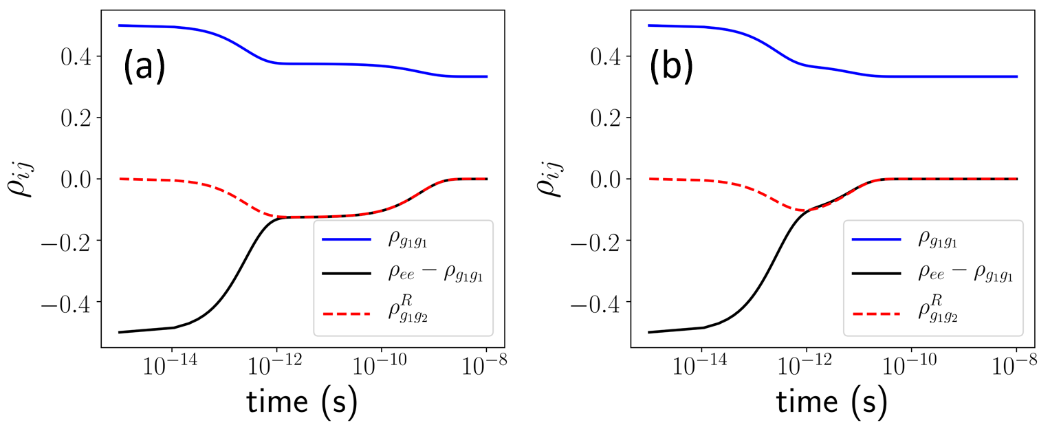
Refer to caption
Figure 5: Population and coherence dynamics of the symmetric Λ\Lambda-system with coherence-free initial state (ρg1​g2R=0\rho^{R}_{g_{1}g_{2}}=0) in the strong-pumping limit ( n¯=103\bar{n}=10^{3}) for Δ/γ=50{\Delta}/{\gamma}=50. The transition dipole alignment parameter pp is set to 1 [panel (a)] and to 0.9 [panel (b)].

To illustrate the interplay between the different coherence-generating and coherence-destroying mechanisms, we plot in Fig. 5 the time evolution of the populations and coherences that enter Eq. (167). The decay of the ground-state population ρe​e\rho_{ee} is accompanied by a steady growth of excited-state populations and coherences. In the quasi-steady state formed on the timescale 1/r<t<τc1/r<t<\tau_{c} the population inversion term ρe​e−ρg1​g1\rho_{ee}-\rho_{g_{1}g_{1}} drives coherence generation. From Fig. 5, we observe the quasisteady state (1) the time evolution of the population difference ρe​e−ρg1​g1\rho_{ee}-\rho_{g_{1}g_{1}} is identical to that of the real part of the coherence ρg1​g2R\rho_{g_{1}g_{2}}^{R} and (2) the imaginary part of the coherence remains constant in time. Setting the left-land side of Eq. (168) to zero, we obtain the imaginary part of the quasisteady coherence as ρg1​g2I=−(Δ/r)​ρg1​g2R\rho_{g_{1}g_{2}}^{I}=-(\Delta/r)\rho^{R}_{g_{1}g_{2}} (we verified this result numerically in the overdamped regime). These considerations allow us to simplify Eq. (167) to yield

ρ˙g1​g2R=−r⁡(1−p+Δ2r2)​ρg1​g2R(t>1/r),\dot{\rho}_{g_{1}g_{2}}^{R}=-r\left(1-p+\frac{\Delta^{2}}{r^{2}}\right)\rho_{g_{1}g_{2}}^{R}\qquad(t>1/r), (169)

which describes coherence decay on the timescale t>1/rt>1/r (note that coherence generation occurs on shorter timescales given by t≃1/rt\simeq 1/r). The simple form of Eq. (169) enables us to introduce an effective decoherence rate γdeff​(p)=r⁡(1−p+Δ2r2)\gamma_{d}^{\text{eff}}(p)=r(1-p+\frac{\Delta^{2}}{r^{2}}) and the effective coherence time

τdeff=1r⁡(1−p+Δ2r2)\tau_{d}^{\text{eff}}=\frac{1}{r(1-p+\frac{\Delta^{2}}{r^{2}})} (170)

The effective decoherence rate model thus establishes that the lifetime of noise-induced coherences is determined by two mechanisms: (1) the interplay between coherence-generating Fano interference and incoherent stimulated emission discussed above [the term r⁡(1−p)r(1-p)] and (2) the coupling between the real and imaginary parts of the coherence [the term Δ2/r\Delta^{2}/r]. The second mechanism is due to the unitary interconversion between the real and imaginary parts of the coherence, which occurs at a rate Δ\Delta. Because the imaginary coherence decays at a rate rr [Eq. (168)], this unitary interconversion makes a small second-order contribution to the overall decay rate proportional to r​Δ2r\Delta^{2}. The two mechanisms contribute equally for p=pceffp=p_{c}^{\text{eff}} where

pceff=1−Δ2r2,p_{c}^{\text{eff}}=1-\frac{\Delta^{2}}{r^{2}}, (171)

which is close to the exact result derived above pc=1−Δ2/r2≃1−12​Δ2r2p_{c}=\sqrt{1-\Delta^{2}/r^{2}}\simeq 1-\frac{1}{2}\frac{\Delta^{2}}{r^{2}} in the overdamped limit (Δ/(n¯​γ)≪1)(\Delta/(\bar{n}\gamma)\ll 1).

Our expression for the effective decoherence rate (170) clarifies the physical origin of the different regimes of coherent dynamics. At p>pceffp>p_{c}^{\text{eff}} the term r⁡(1−p)r(1-p) is small compared with Δ2/r2\Delta^{2}/r^{2}, the rate of coherence generation (via Fano interference) and decay (via incoherent stimulated emission) are almost exactly balanced. As a result, the effective decoherence rate is dominated by the second-order mechanism (2) and Eq. (170) yields τdeff=r/Δ2=n¯​γ/Δ2\tau_{d}^{\text{eff}}={r}/{\Delta^{2}}=\bar{n}\gamma/\Delta^{2}, which is identical to the exact result to within the factor 1.34. Remarkably, the effective decoherence model correctly predicts the linear scaling of the coherence lifetime with both n¯\bar{n} and Δ/γ\Delta/\gamma in the p>pcp>p_{c} regime.

We note that the transition dipole alignment parameter pp can be thought of as controlling the relative contribution of mechanisms (1) and (2) leading to the overall effective decoherence rate (170). In the strong-pumping regime, mechanism (1) is much more efficient in destroying the coherence than mechanism (2). Significantly, mechanism (1) is pp-dependent and can be suppressed by taking p→1p\to 1, leading to the long-lived coherent regime governed by mechanism (2).

I.7 Weak pumping regime

In this section we will specifically consider the weak pumping limit, where incoherent driving is much slower than spontaneous decay (r≪γr\ll\gamma). In this regime, the average photon number of the radiation field is small (n¯≪1\bar{n}\ll 1).

I.7.1 Solving the equation D=0D=0 in the weak pumping limit

For small Δγ\frac{\Delta}{\gamma} and n¯\bar{n}, the discriminant in Eq. (19) is well represented by the zeroth and second order terms d0d_{0}, d2​n¯2d_{2}\bar{n}^{2} only, and it can be written as

D=γ62916​(d0+d2​n¯2)D=\frac{\gamma^{6}}{2916}\big(d_{0}+d_{2}\bar{n}^{2}\big) (172)

where d0d_{0}, and d2d_{2} are the expansion coefficients listed in Table I, which are further simplified as

d0\displaystyle d_{0} =108​(Δγ)2​[(Δγ)2+4]2\displaystyle=108\Big(\frac{\Delta}{\gamma}\Big)^{2}\Big[\Big(\frac{\Delta}{\gamma}\Big)^{2}+4\Big]^{2}
d2\displaystyle d_{2} =−9​(47+108​p2)​(Δγ)4+72​(64+87​p2+18​p4)​(Δγ)2−432​p4\displaystyle=-9(47+108p^{2})\Big(\frac{\Delta}{\gamma}\Big)^{4}+72(64+87p^{2}+18p^{4})\Big(\frac{\Delta}{\gamma}\Big)^{2}-432p^{4} (173)

Our goal is to find a relationship between Δγ\frac{\Delta}{\gamma} and n¯\bar{n} by solving the equation D=0D=0. Using the expansion coefficients in Eq. (173), Eq. (172) can be recast

n¯2\displaystyle\bar{n}^{2} =−d0d2=108​(Δγ)2​[(Δγ)2+4]2[9​(47+108​p2)​(Δγ)4−72​(64+87​p2+18​p4)​(Δγ)2+432​p4]\displaystyle=-\frac{d_{0}}{d_{2}}=\frac{108\Big(\frac{\Delta}{\gamma}\Big)^{2}\Big[\Big(\frac{\Delta}{\gamma}\Big)^{2}+4\Big]^{2}}{\Big[9(47+108p^{2})\Big(\frac{\Delta}{\gamma}\Big)^{4}-72(64+87p^{2}+18p^{4})\Big(\frac{\Delta}{\gamma}\Big)^{2}+432p^{4}\Big]} (174)

We rearrange the above equation to obtain the ratio of (Δ/γ)(\Delta/\gamma) to n¯\bar{n} in the following form

1n¯2​(Δγ)2\displaystyle\frac{1}{\bar{n}^{2}}\Big(\frac{\Delta}{\gamma}\Big)^{2} =[9​(47+108​p2)​(Δγ)4−72​(64+87​p2+18​p4)​(Δγ)2+432​p4]108​[(Δγ)2+4]2\displaystyle=\frac{\Big[9(47+108p^{2})\Big(\frac{\Delta}{\gamma}\Big)^{4}-72(64+87p^{2}+18p^{4})\Big(\frac{\Delta}{\gamma}\Big)^{2}+432p^{4}\Big]}{108\Big[\Big(\frac{\Delta}{\gamma}\Big)^{2}+4\Big]^{2}} (175)

For small values of Δ/γ\Delta/\gamma, we can neglect the (Δ/γ)2(\Delta/\gamma)^{2} and (Δ/γ)4(\Delta/\gamma)^{4} terms on the right-hand side to obtain

(Δr)2=p44\Big(\frac{\Delta}{r}\Big)^{2}=\frac{p^{4}}{4} (176)

Finally, we take the square root on both sides of Eq. (176) to find the equation for the critical line

Δr=p22\frac{\Delta}{r}=\frac{p^{2}}{2} (177)
Refer to caption
Figure 6: (a) A contour plot of the discriminant DD for small Δ/γ\Delta/\gamma and n¯\bar{n} and p=1.0p=1.0. (b) An expanded view of the region close to the origin (Δ/γ≪1\Delta/\gamma\ll 1, n¯≪1\bar{n}\ll 1 and p=1.0p=1.0).

Therefore, for small values of Δγ\frac{\Delta}{\gamma} and n¯\bar{n}, the critical line is a straight line with the slope given by m=p2/2m=p^{2}/2. The dynamical regimes for small n¯\bar{n} are illustrated in the contour plot of Fig. 6(a), (b), which displays that the line of zero discriminant passes through the origin. The underdamped and overdamped regimes are defined by the conditions Δr>p22\frac{\Delta}{r}>\frac{p^{2}}{2} and Δr<p22\frac{\Delta}{r}<\frac{p^{2}}{2}, respectively. Because one expects Δ/r>1\Delta/r>1 to be the case for very small rr, overdamped dynamics are strongly suppressed in the weak pumping limit.

For completeness, we also consider the case of the weakly driven degenerate Λ\Lambda-system (Δ=0\Delta=0), where the zeroth and first order coefficients d0​(p)d_{0}(p) and d1​(p)d_{1}(p) in Eq. (19) vanish and the discriminant becomes

D=−432​p2​n¯2D=-432p^{2}\bar{n}^{2} (178)

The discriminant is always negative for p≠0p\neq 0. This implies that the degenerate Λ\Lambda-system always exhibits dynamics either in the overdamped regime (p≠0p\neq 0) or the critical regime (p=0p=0). This is in contrast to the weakly driven non-degenerate Λ\Lambda-system considered above, whose dynamics are primarily in the underdamped regime.

In the strong pumping regime, the discriminant (19) of the degenerate Λ\Lambda-system becomes

D=−108​p2​n¯2​[4+4​p2​(5+2​p2)​n¯+p2​(37+36​p2)​n¯2+6​p2​(5+9​p2)​n¯3+9​p2​(1+3​p2)​n¯4]D=-108p^{2}\bar{n}^{2}\big[4+4p^{2}(5+2p^{2})\bar{n}+p^{2}(37+36p^{2})\bar{n}^{2}+6p^{2}(5+9p^{2})\bar{n}^{3}+9p^{2}(1+3p^{2})\bar{n}^{4}\big] (179)

We observe that the discriminant is either zero or negative. Thus, the dynamics of the strongly driven degenerate Λ\Lambda-system are restricted to either overdamped (p≠0p\neq 0) or critical (p=0p=0) regimes. This is again different from the strongly driven non-degenerate Λ\Lambda-system, which shows dynamics in all three regimes.

I.7.2 Eigenvalues and coherence lifetimesin the underdamped regime [Δ/r>p2/2\Delta/r>p^{2}/2]

The eigenvalues in the weak pumping regime can be expressed as a polynomial function of n¯≪1\bar{n}\ll 1 (see above)

λj=γ​∑k=05z~j​k​n¯k​(j=1−3).\lambda_{j}=\gamma\sum_{k=0}^{5}\tilde{z}_{jk}\bar{n}^{k}\kern 5.0pt(j=1-3). (180)

Neglecting the terms with k>2k>2 we find

λj=γ⁡[z~j​0+z~j​1​n¯+z~j​2​n¯2]​(j=1−3).\lambda_{j}=\gamma\big[\tilde{z}_{j0}+\tilde{z}_{j1}\bar{n}+\tilde{z}_{j2}\bar{n}^{2}\big]\kern 5.0pt(j=1-3). (181)

Equation (181) is a general expression for the eigenvalues of the coefficient matrix (9) in the weak pumping limit. The above expression is valid for n¯≤0.01\bar{n}\leq 0.01 and it converges quickly with n¯\bar{n}. The expansion coefficients z~j​k\tilde{z}_{jk} are listed in Table XIII.

Refer to caption
Figure 7: Relative contributions of the different terms to the eigenvalues λ1\lambda_{1} (a), Real (b) and Imaginary (c) part of λ2\lambda_{2} plotted as a function of Δ/γ\Delta/\gamma in the weak pumping limit with n¯=10−3\bar{n}=10^{-3} and p=1p=1. Note that λ3\lambda_{3} is complex conjugate of λ2\lambda_{2}.

Next we compare the relative contributions of the different z~j​k​n¯k\tilde{z}_{jk}\bar{n}^{k} terms in Eq. (181) as a function of Δ/γ\Delta/\gamma in Figure 7. From Fig. 7(a), we observe that the zeroth order term z~10\tilde{z}_{10} is the dominant term for |λ1||\lambda_{1}| which can be written as

λ1=|z~10|​γ,\lambda_{1}=|\tilde{z}_{10}|\gamma, (182)

where the pp-dependent coefficient z~10\tilde{z}_{10} is listed in Table XIII.

Similarly, the real and imaginary parts of the eigenvalue λ2\lambda_{2} as a function of Δ/γ\Delta/\gamma are plotted in Figs. 7(b) and (c). We see that the imaginary part of |Im​(λ2)||\text{Im}(\lambda_{2})| depends significantly on the zeroth order term (Im​(z~20)\text{Im}(\tilde{z}_{20})) similar to λ1\lambda_{1}. However, it is the first-order term Re​(z~20)​n¯\text{Re}(\tilde{z}_{20})\bar{n} that is dominant in the real part of |Re​(λ2)||\text{Re}(\lambda_{2})|. This approximation permits us to express the real and imaginary parts of λ2\lambda_{2} in the following form

Re​(λ2)\displaystyle\text{Re}(\lambda_{2}) =Re​(z~21)​r,\displaystyle=\text{Re}(\tilde{z}_{21})r,
Im​(λ2)\displaystyle\text{Im}(\lambda_{2}) =Im​(z~20)​γ,\displaystyle=\text{Im}(\tilde{z}_{20})\gamma, (183)

where the coefficients z~20\tilde{z}_{20} and z~21\tilde{z}_{21} are listed in Table XIII. Here, we note that the eigenvalue λ3\lambda_{3} exhibits same features as λ2\lambda_{2} as they are complex conjugates of each other.

The eigenvalues in the weak pumping regime can be evaluated more simply by assuming the decoupling of the coherence term in Eq. (1). This is a valid assumption for the strong pumping regime (Δ/r≥1\Delta/r\geq 1) as long as Δ/γ>1\Delta/\gamma>1. In the weak pumping limit with Δ/γ>1\Delta/\gamma>1, the coefficient matrix (62) after diagonalization results in the following three eigenvalues

λ1\displaystyle\lambda_{1} =−2​γ\displaystyle=-2\gamma (184)
λ2\displaystyle\lambda_{2} =−r+i​Δ\displaystyle=-r+i\Delta (185)
λ3\displaystyle\lambda_{3} =−r−i​Δ\displaystyle=-r-i\Delta (186)

The eigenvalue spectrum λk\lambda_{k} of the coefficient matrix A consists of one real and two complex conjugate eigenvalues. Thus, the dynamics of the Λ\Lambda-system weakly driven by incoherent radiation is in the underdamped regime as discussed above. It is important to note that we can not neglect the incoherent driving rate rr in the eigenvalues λ2,3\lambda_{2,3} in spite of its small magnitude in the weak pumping limit.

If the ground state splitting is small in comparison to the spontaneous decay rate (Δ/γ<1\Delta/\gamma<1), the eigenvalue (184) is in complete agreement with the eigenvalue evaluated in (182). However, the eigenvalues (185)-(186) deviate from the exact values. Next, we compute the eigenvalues (λ2\lambda_{2}) using Eq. (181) for which the expansion coefficients z~2​k\tilde{z}_{2k} are evaluated with (α2,β2)=(ω2,ω)(\alpha_{2},\beta_{2})=(\omega^{2},\omega).

Substituting the coefficients z~2​k\tilde{z}_{2k}, ω=(−1+i​3)/2\omega=(-1+i\sqrt{3})/2, ω2=(−1−i​3)/2\omega^{2}=(-1-i\sqrt{3})/2 in Eq. (183), we obtain

Re​(λ2)\displaystyle\text{Re}(\lambda_{2}) =r⁡{−53+16​K~​(8+6​p2)+118​K~​(3​Δ2γ2−4)​t1+118​K~​t1}\displaystyle=r\bigg\{-\frac{5}{3}+\frac{1}{6\tilde{K}}(8+6p^{2})+\frac{1}{18\tilde{K}}\Big(3\frac{\Delta^{2}}{\gamma^{2}}-4\Big)t_{1}+\frac{1}{18}\tilde{K}t_{1}\bigg\} (187)
Im​(λ2)\displaystyle\text{Im}(\lambda_{2}) =−3γ{16​K~(3Δ2γ2−4)+K~6)}\displaystyle=-\sqrt{3}\gamma\bigg\{\frac{1}{6\tilde{K}}\Big(3\frac{\Delta^{2}}{\gamma^{2}}-4\Big)+\frac{\tilde{K}}{6}\bigg)\bigg\} (188)
Refer to caption
Figure 8: The real (a) and imaginary (b) parts of the eigenvalue λ2\lambda_{2} in Eqs. (187) and (188) vs. Δ/γ\Delta/\gamma for n¯=10−3\bar{n}=10^{-3} and p=1p=1.

Figure 8 displays the absolute values of the real and imaginary parts of (λ2\lambda_{2}) as a function of Δ/γ\Delta/\gamma for p=1p=1. We observe from Fig. 8(a) that the real part of λ2\lambda_{2} increases by a factor of two when going from the region of large to small ground state splitting. Furthermore, the real part of λ2\lambda_{2} attains asymptotic limits for large and small Δ/γ\Delta/\gamma. In contrast, the imaginary part of the eigenvalue λ2\lambda_{2} is a constant, equal to the ground state splitting (Δ\Delta), for a wide range of Δ/γ\Delta/\gamma (10−2≤Δ/γ≤10210^{-2}\leq\Delta/\gamma\leq 10^{2}) as shown in Fig. 8(b).

To evaluate the real part of λ2\lambda_{2} at the limiting values of Δ/γ\Delta/\gamma, we first consider the case of large Δ/γ≫1\Delta/\gamma\gg 1. We begin by evaluating the various terms that define λ2\lambda_{2}

c0\displaystyle c_{0} =36​(Δγ)2,d0=108​(Δγ)6,K~=3​(Δγ),b0=3​(Δγ)2,b1=−(8+6​p2),t1=2​3(Δγ)\displaystyle=36(\frac{\Delta}{\gamma})^{2},\kern 5.0ptd_{0}=108(\frac{\Delta}{\gamma})^{6},\kern 5.0pt\tilde{K}=\sqrt{3}(\frac{\Delta}{\gamma}),\kern 5.0ptb_{0}=3(\frac{\Delta}{\gamma})^{2},\kern 5.0ptb_{1}=-(8+6p^{2}),\kern 5.0ptt_{1}=\frac{2\sqrt{3}}{(\frac{\Delta}{\gamma})} (189)

Using Eq. (189) in Eq. (187), we find

Re​(λ2)\displaystyle\text{Re}(\lambda_{2}) =r⁡[−53−12​{−(8+6​p2)3​K~−3​(Δγ)2​t19​K~}+118​3​(Δγ)​t1]\displaystyle=r\bigg[-\frac{5}{3}-\frac{1}{2}\bigg\{\frac{-(8+6p^{2})}{3\tilde{K}}-\frac{3(\frac{\Delta}{\gamma})^{2}t_{1}}{9\tilde{K}}\bigg\}+\frac{1}{18}\sqrt{3}\Big(\frac{\Delta}{\gamma}\Big)t_{1}\bigg]
=r⁡[−53+16​K~​{(8+6​p2)+(Δγ)2​2​3(Δγ)}+118​3​(Δγ)​2​3(Δγ)]\displaystyle=r\bigg[-\frac{5}{3}+\frac{1}{6\tilde{K}}\bigg\{(8+6p^{2})+\Big(\frac{\Delta}{\gamma}\Big)^{2}\frac{2\sqrt{3}}{(\frac{\Delta}{\gamma})}\bigg\}+\frac{1}{18}\sqrt{3}\Big(\frac{\Delta}{\gamma}\Big)\frac{2\sqrt{3}}{(\frac{\Delta}{\gamma})}\bigg]
=r⁡[−53+16​3​(Δγ)​{(8+6​p2)+2​3​(Δγ)}+13]\displaystyle=r\bigg[-\frac{5}{3}+\frac{1}{6\sqrt{3}(\frac{\Delta}{\gamma})}\bigg\{(8+6p^{2})+2\sqrt{3}\Big(\frac{\Delta}{\gamma}\Big)\bigg\}+\frac{1}{3}\bigg]
=r⁡[−43+16​3​(Δγ)​(8+6​p2)+13]=r⁡[−1+16​3​(Δγ)​(8+6​p2)]=−r\displaystyle=r\bigg[-\frac{4}{3}+\frac{1}{6\sqrt{3}(\frac{\Delta}{\gamma})}(8+6p^{2})+\frac{1}{3}\bigg]=r\bigg[-1+\frac{1}{6\sqrt{3}(\frac{\Delta}{\gamma})}(8+6p^{2})\bigg]=-r (190)

where we have neglected the last term 16​3​(Δγ)​(8+6​p2)\frac{1}{6\sqrt{3}(\frac{\Delta}{\gamma})}(8+6p^{2}) for large Δ/γ\Delta/\gamma. From Eq. (190), we observe that real part of the eigenvalue λ2\lambda_{2} is independent of the dipole alignment factor (pp), and takes the asymptotic value of rr as seen in Fig. 8(a).

Next we calculate the real part of eigenvalue λ2\lambda_{2} when Δ/γ≪1\Delta/\gamma\ll 1. We proceed by finding the terms relevant for λ2\lambda_{2} as in the previous case

c0\displaystyle c_{0} =16,d0=0,K~=2,b0=−4,b1=−(8+6​p2),t1=(12+9​p2)4\displaystyle=16,\kern 5.0ptd_{0}=0,\kern 5.0pt\tilde{K}=2,\kern 5.0ptb_{0}=-4,\kern 5.0ptb_{1}=-(8+6p^{2}),\kern 5.0ptt_{1}=\frac{(12+9p^{2})}{4} (191)

Using Eq. (191) in Eq. (187), we find

Re​(λ2)\displaystyle\text{Re}(\lambda_{2}) =r⁡[−53−12​{−(8+6​p2)3​K~−−4​(12+9​p2)49​K~}+118​K~​(12+9​p2)4]\displaystyle=r\bigg[-\frac{5}{3}-\frac{1}{2}\bigg\{\frac{-(8+6p^{2})}{3\tilde{K}}-\frac{-4\frac{(12+9p^{2})}{4}}{9\tilde{K}}\bigg\}+\frac{1}{18}\tilde{K}\frac{(12+9p^{2})}{4}\bigg]
=r⁡[−53+112​(8+6​p2)+136​(12+9​p2)−136​(12+9​p2)]\displaystyle=r\bigg[-\frac{5}{3}+\frac{1}{12}(8+6p^{2})+\frac{1}{36}(12+9p^{2})-\frac{1}{36}(12+9p^{2})\bigg]
=r⁡[−53+112​(8+6​p2)]=r⁡[(p2−2)2]\displaystyle=r\bigg[-\frac{5}{3}+\frac{1}{12}(8+6p^{2})\bigg]=r\bigg[\frac{(p^{2}-2)}{2}\bigg] (192)

The above expression shows that Re​(λ2)\text{Re}(\lambda_{2}) depends on the dipole alignment factor pp. In the absence of Fano coherence (p=0p=0), Re​(λ2)=−r\text{Re}(\lambda_{2})=-r and with full Fano coherence (p=1p=1), Re(λ2)=−r/2\text{Re}(\lambda_{2})=-r/2 as demonstrated in Fig. 8(a). This result shows that the coherence time, which is the inverse of the absolute value of the real part of the eigenvalue λ2\lambda_{2}, is enhanced two-fold in the presence of Fano coherence when the ground state splitting is small (Δ≤γ\Delta\leq\gamma).

I.7.3 Population and Coherence dynamics in the underdamped regime [Δ/r>p2/2\Delta/r>p^{2}/2]

Here, we derive the analytical solutions of the BR equations for a weakly driven Λ\Lambda-system. For r≪γr\ll\gamma and r≪Δr\ll\Delta, the excited-state population and coherences [see, e.g, Eq. (I.5.3)] can be further simplified as

ρg1​g1​(t)\displaystyle\rho_{g_{1}g_{1}}(t) =12​e−2​γ​t+(r+γ3​r+2​γ)​(1−e−2​γ​t)=r+γ(3​r+2​γ)+r2​(3​r+2​γ)​e−2​γ​t\displaystyle=\frac{1}{2}\text{e}^{-2\gamma t}+\bigg(\frac{r+\gamma}{3r+2\gamma}\bigg)(1-\text{e}^{-2\gamma t})=\frac{r+\gamma}{(3r+2\gamma)}+\frac{r}{2(3r+2\gamma)}\text{e}^{-2\gamma t} (193)
ρg1​g2R​(t)\displaystyle\rho_{g_{1}g_{2}}^{R}(t) =p​r2​[4​γ2+Δ2]​[2​γ​e−2​γ​t−{2​γ​cos⁡Δ​t+Δ​sin⁡Δ​t}​e−r​t]\displaystyle=\frac{pr}{2[4\gamma^{2}+\Delta^{2}]}\bigg[2\gamma\text{e}^{-2\gamma t}-\big\{2\gamma\cos\Delta t+\Delta\sin\Delta t\big\}\text{e}^{-rt}\bigg] (194)
ρg1​g2I​(t)\displaystyle\rho_{g_{1}g_{2}}^{I}(t) =p​r2​[4​γ2+Δ2]​[Δ​e−2​γ​t+{2​γ​sin⁡Δ​t−Δ​cos⁡Δ​t}​e−r​t]\displaystyle=\frac{pr}{2[4\gamma^{2}+\Delta^{2}]}\bigg[\Delta\text{e}^{-2\gamma t}+\big\{2\gamma\sin\Delta t-\Delta\cos\Delta t\big\}\text{e}^{-rt}\bigg] (195)
Refer to caption
Figure 9: Numerical [blue solid line] vs analytical [red dashed line] solutions of BR equations (1) - (2) in the underdamped regime. (a) Excited-state population [(a)] and coherence [(b), (c)] dynamics of the symmetric Λ\Lambda-system irradiated by incoherent light in the weak pumping limit with n¯=10−3\bar{n}=10^{-3} and Δ/γ=10{\Delta}/{\gamma}=10.
Refer to caption
Figure 10: Numerical [blue solid line] vs analytical [red dashed line] solutions of BR equations (1) - (2) in the underdamped regime. (a) Excited-state population [(a)] and coherence [(b), (c)] dynamics of the symmetric Λ\Lambda-system irradiated by incoherent light in the weak pumping limit with n¯=10−3\bar{n}=10^{-3} and Δ/γ=10−1{\Delta}/{\gamma}=10^{-1}.

Equations (193) - (195) give the exact population and coherence dynamics of the weakly driven Λ\Lambda-system when the ground state splitting is large in comparison to the spontaneous decay rate (Δ>γ\Delta>\gamma). Figure 9 shows a nearly perfect agreement of the analytical and numerical solutions for Δ>γ\Delta>\gamma. From the above equations, we note that there are two separate time scales 1/2​γ1/2\gamma and 1/r1/r for the evolution of coherence. Figure 9(b) - (c) exhibits the emergence of coherence from the coherence-free initial state which oscillates with a frequency of Δ\Delta that decays on the timescale 1/r1/r.

However, the analytical and numerical solutions for Δ/γ≤1\Delta/\gamma\leq 1 displayed in Fig. 10 disagree at later times. This discrepancy can be understood from the behavior of λ2,3\lambda_{2,3} as a function of Δ/γ\Delta/\gamma discussed in the previous section. While Im​(λ2,3)=Δ\text{Im}(\lambda_{2,3})=\Delta for a wide range of Δ/γ\Delta/\gamma, Re​(λ2,3)\text{Re}(\lambda_{2,3}) vary from rr to r/2r/2 as Δ/γ\Delta/\gamma decreases. This implies that the coherences decay on the time scale 2/r2/r when Δ/γ<1\Delta/\gamma<1. In this limit, the analytical solutions for coherence dynamics takes the form

ρg1​g2R​(t)\displaystyle\rho_{g_{1}g_{2}}^{R}(t) =p​r2​[4​γ2+Δ2]​[2​γ​e−2​γ​t−{2​γ​cos⁡Δ​t+Δ​sin⁡Δ​t}​e−r2​t]\displaystyle=\frac{pr}{2[4\gamma^{2}+\Delta^{2}]}\bigg[2\gamma\text{e}^{-2\gamma t}-\big\{2\gamma\cos\Delta t+\Delta\sin\Delta t\big\}{e}^{-\frac{r}{2}t}\bigg] (196)
ρg1​g2I​(t)\displaystyle\rho_{g_{1}g_{2}}^{I}(t) =p​r2​[4​γ2+Δ2]​[Δ​e−2​γ​t+{2​γ​sin⁡Δ​t−Δ​cos⁡Δ​t}​e−r2​t]\displaystyle=\frac{pr}{2[4\gamma^{2}+\Delta^{2}]}\bigg[\Delta\text{e}^{-2\gamma t}+\big\{2\gamma\sin\Delta t-\Delta\cos\Delta t\big\}\text{e}^{-\frac{r}{2}t}\bigg] (197)

To interpolate between the two limits, we introduce a dimensionless function Q⁡(x)=R​e​(λ2)/rQ(x)=Re(\lambda_{2})/r plotted in Fig. 8(a), in terms of which

ρg1​g2R​(t)\displaystyle\rho_{g_{1}g_{2}}^{R}(t) =p​r2​[4​γ2+Δ2]​[2​γ​e−2​γ​t−{2​γ​cos⁡Δ​t+Δ​sin⁡Δ​t}​e−r​Q​(Δγ)​t]\displaystyle=\frac{pr}{2[4\gamma^{2}+\Delta^{2}]}\bigg[2\gamma\text{e}^{-2\gamma t}-\big\{2\gamma\cos\Delta t+\Delta\sin\Delta t\big\}\text{e}^{-{r}{Q(\frac{\Delta}{\gamma}})t}\bigg] (198)
ρg1​g2I​(t)\displaystyle\rho_{g_{1}g_{2}}^{I}(t) =p​r2​[4​γ2+Δ2]​[Δ​e−2​γ​t+{2​γ​sin⁡Δ​t−Δ​cos⁡Δ​t}​e−r​Q​(Δγ)​t].\displaystyle=\frac{pr}{2[4\gamma^{2}+\Delta^{2}]}\bigg[\Delta\text{e}^{-2\gamma t}+\big\{2\gamma\sin\Delta t-\Delta\cos\Delta t\big\}\text{e}^{-{r}{Q(\frac{\Delta}{\gamma}})t}\bigg]. (199)

We finally consider a weakly driven Λ\Lambda-system with the ground states initially in an equal coherent superposition. For r≪γr\ll\gamma and r≪Δr\ll\Delta, the coherent dynamics governed by Eq. (166) can be recast as

ρg1​g2R​(t)=[ρRg1​g2(0)cosΔt+ρIg1​g2(0)sinΔt)]e−r​t+p​r2​[4​γ2+Δ2][2γe−2​γ​t−{2γcosΔt+ΔsinΔt}e−r​t]\displaystyle\begin{split}\rho_{g_{1}g_{2}}^{R}(t)&=\big[\rho^{R}_{g_{1}g_{2}}(0)\cos\Delta t+\rho^{I}_{g_{1}g_{2}}(0)\sin\Delta t)\big]\text{e}^{-rt}+\frac{pr}{2[4\gamma^{2}+\Delta^{2}]}\bigg[2\gamma\text{e}^{-2\gamma t}-\Big\{2\gamma\cos\Delta t+\Delta\sin\Delta t\Big\}\text{e}^{-rt}\bigg]\end{split}
ρg1​g2I​(t)=[−ρRg1​g2(0)sinΔt+ρIg1​g2(0)cosΔt]e−r​t+p​r2​[4​γ2+Δ2][Δe−2​γ​t+{2γ)sinΔt−ΔcosΔt}e−r​t]\displaystyle\begin{split}\rho_{g_{1}g_{2}}^{I}(t)&=\big[-\rho^{R}_{g_{1}g_{2}}(0)\sin\Delta t+\rho^{I}_{g_{1}g_{2}}(0)\cos\Delta t\big]\text{e}^{-rt}+\frac{pr}{2[4\gamma^{2}+\Delta^{2}]}\bigg[\Delta\text{e}^{-2\gamma t}+\Big\{2\gamma)\sin\Delta t-\Delta\cos\Delta t\Big\}\text{e}^{-rt}\bigg]\end{split} (200)

Equations (200) accurately describe the coherent dynamics of a weakly driven Λ\Lambda-system if the ground state splitting is greater than the spontaneous decay rate (Δ>γ\Delta>\gamma). However, in the opposite limit (Δ≤γ\Delta\leq\gamma) these analytical solutions deviate from numerical solutions at later times. Following the same procedure as described above, we introduce a dimensionless function Q⁡(x)=R​e​(λ2)/rQ(x)=Re(\lambda_{2})/r that interpolates between the two limits of the eigenvalue λ2\lambda_{2} to find the general solutions in the form

ρg1​g2R​(t)=[ρRg1​g2(0)cosΔt+ρIg1​g2(0)sinΔt)]e−r​Q​(Δγ)​t+p​r2​[4​γ2+Δ2][2γe−2​γ​t−{2γcosΔt+ΔsinΔt}e−r​Q​(Δγ)​t]\displaystyle\begin{split}\rho_{g_{1}g_{2}}^{R}(t)&=\big[\rho^{R}_{g_{1}g_{2}}(0)\cos\Delta t+\rho^{I}_{g_{1}g_{2}}(0)\sin\Delta t)\big]\text{e}^{-rQ(\frac{\Delta}{\gamma})t}+\frac{pr}{2[4\gamma^{2}+\Delta^{2}]}\bigg[2\gamma\text{e}^{-2\gamma t}-\Big\{2\gamma\cos\Delta t+\Delta\sin\Delta t\Big\}\text{e}^{-rQ(\frac{\Delta}{\gamma})t}\bigg]\end{split}
ρg1​g2I​(t)=[−ρg1​g2R​(0)​sin⁡Δ​t+ρg1​g2I​(0)​cos⁡Δ​t]​e−r​Q​(Δγ)​t+p​r2​[4​γ2+Δ2]​[Δ​e−2​γ​t+{2​γ​sin⁡Δ​t−Δ​cos⁡Δ​t}​e−r​Q​(Δγ)​t]\displaystyle\begin{split}\rho_{g_{1}g_{2}}^{I}(t)&=\big[-\rho^{R}_{g_{1}g_{2}}(0)\sin\Delta t+\rho^{I}_{g_{1}g_{2}}(0)\cos\Delta t\big]\text{e}^{-rQ(\frac{\Delta}{\gamma})t}+\frac{pr}{2[4\gamma^{2}+\Delta^{2}]}\bigg[\Delta\text{e}^{-2\gamma t}+\Big\{2\gamma\sin\Delta t-\Delta\cos\Delta t\Big\}\text{e}^{-rQ(\frac{\Delta}{\gamma})t}\bigg]\end{split} (201)

This completes the derivation of Eqs. (4) of the main text.

I.8 von Neumann Entropy

Here, we describe the procedure of computing the von Neumann entropy of the quantum states generated by incoherent driving of the Λ\Lambda-system. The von Neumann entropy of a quantum system described by the density operator ρ\rho is defined as

𝒮​(t)=−Tr​(ρ​ln​ρ)\mathcal{S}(t)=-\text{Tr}(\rho\text{ln}\rho) (202)

where Tr is the trace operation.

By diagonalizing the density operator we can express it in the following form

ρ=∑iλi​|i⟩​⟨i|\rho=\sum_{i}\lambda_{i}\ket{i}\bra{i} (203)

where |i⟩\ket{i} is the eigenvector of ρ\rho with the eigenvalue λi\lambda_{i}. The von-Neumann entropy in the eigenbasis of ρ\rho then becomes

𝒮(t)=−∑iλilnλi\mathcal{S}(t)=-\sum_{i}\lambda_{i}\text{ln}{\lambda_{i}} (204)

The density operator of the Λ\Lambda-system driven by incoherent light in the energy eigenbasis is

ρ=(ρe​e000ρg1​g1ρg1​g20ρg2​g1ρg2​g2)\rho=\begin{pmatrix}\rho_{ee}&0&0\\ 0&\rho_{g_{1}g_{1}}&\rho_{g_{1}g_{2}}\\ 0&\rho_{g_{2}g_{1}}&\rho_{g_{2}g_{2}}\end{pmatrix} (205)
Refer to caption
Figure 11: Comparison of von Neumann Entropy defined in Eq. (208) with full Fano coherence [blue solid line] vs without Fano coherence [red dashed line] as a function of time in the weak pumping limit with n¯=10−3\bar{n}=10^{-3}. (a) Panels [(a)] and [(b)] display the evolution of the von Neumann entropy with Δ/γ=10−1\Delta/\gamma=10^{-1} and 10−210^{-2}, and the ground states of the Λ\Lambda-system initially in a coherent superposition. (b) Panel [(c)] von Neumann entropy is evaluated for Δ/γ=10−1\Delta/\gamma=10^{-1}, and no initial coherence between the ground states. (c) Panel [(d)] same as panels[(b)]-[(c)] for Δ/γ=10\Delta/\gamma=10. Note that time is given in the units of r−1r^{-1}.

The eigenvalues of ρ\rho are

λ1\displaystyle\lambda_{1} =ρe​e\displaystyle=\rho_{ee}
λ2,3\displaystyle\lambda_{2,3} =12​[(ρg1​g1+ρg2​g2)±(ρg1​g1−ρg2​g2)2+4​ρg1​g2​ρg2​g1]\displaystyle=\frac{1}{2}\Big[\big(\rho_{g_{1}g_{1}}+\rho_{g_{2}g_{2}}\big)\pm\sqrt{\big(\rho_{g_{1}g_{1}}-\rho_{g_{2}g_{2}}\big)^{2}+4\rho_{g_{1}g_{2}}\rho_{g_{2}g_{1}}}\Big] (206)

For the symmetric Λ\Lambda-system, these expressions simplify to

λ1\displaystyle\lambda_{1} =ρe​e\displaystyle=\rho_{ee}
λ2,3\displaystyle\lambda_{2,3} =ρg1​g1±|ρg1​g2|\displaystyle=\rho_{g_{1}g_{1}}\pm|\rho_{g_{1}g_{2}}| (207)

Plugging Eqs. (I.8) into Eq. (204), we obtain the von-Neumann entropy of the symmetric Λ\Lambda-system

𝒮⁡(t)=−[(ρg1​g1+|ρg1​g2|)​ln​(ρg1​g1+|ρg1​g2|)+(ρg1​g1−|ρg1​g2|)​ln​(ρg1​g1−|ρg1​g2|)+ρe​e​ln​ρe​e]\mathcal{S}(t)=-\Big[\big(\rho_{g_{1}g_{1}}+|\rho_{g_{1}g_{2}}|\big)\text{ln}\big(\rho_{g_{1}g_{1}}+|\rho_{g_{1}g_{2}}|\big)+\big(\rho_{g_{1}g_{1}}-|\rho_{g_{1}g_{2}}|\big)\text{ln}\big(\rho_{g_{1}g_{1}}-|\rho_{g_{1}g_{2}}|\big)+\rho_{ee}\text{ln}\rho_{ee}\Big] (208)

Substituting the time-dependent density matrix elements calculated above, we obtain the time evolution of von Neumann entropy in the weak and strong pumping limits plotted in Figs. 11 and 12, respectively.

Refer to caption
Figure 12: von Neumann Entropy defined in Eq. (208) with full Fano coherence [blue solid line] vs without Fano coherence [red dashed line] as a function of time in the strong pumping limit. (a) Panels [(a)] and [(b)] display the evolution of von Neumann entropy for n¯=103\bar{n}=10^{3}, Δ/γ=102\Delta/\gamma=10^{2} with no initial coherence between the ground states, and the ground states initially in an equal coherent superposition. (b) Panels [(c)] and [(d)] show the evolution of von Neumann entropy for n¯=102\bar{n}=10^{2}, Δ/γ=103\Delta/\gamma=10^{3} with no initial coherence between the ground states, and the ground states initially in a coherent superposition. Note that time is given in the units of γ−1\gamma^{-1}.

II Λ\Lambda-system driven by polarized incoherent light: The Bloch-Redfield equations and the steady-state solution

II.1 Bloch-Redfield equations for a Λ\Lambda-system driven by polarized incoherent radiation

Consider a beam of He∗ atoms irradiated by incoherent light, propagating along the z{{z}}-direction, and linearly polarized in the x{{x}}-direction. A uniform magnetic field applied in the z{z}-direction produces a tunable Zeeman shift between the ground states Δ=2​μB​Bz\Delta=2\mu_{B}B_{z}, where μB\mu_{B} is the Bohr magneton and BzB_{z} is the magnitude of the applied magnetic field. Due to the polarized nature of the radiation field, the average number of photons depends on the direction of propagation 𝒌^=k/k\hat{\bm{k}}=\textbf{k}/k

⟨nk,λ⟩=δk^,z^​δ𝜺k​λ,x^​n¯k,\langle n_{\textbf{k},\lambda}\rangle=\delta_{\hat{\textbf{k}},\hat{\textbf{z}}}\kern 5.0pt\delta_{\bm{\varepsilon}_{\textbf{k}\lambda},\hat{\textbf{x}}}\kern 5.0pt\bar{n}_{k}, (209)

where n¯k\bar{n}_{k} is the average photon number of the radiation field, k is the wave-vector, λ\lambda is the polarization mode index and 𝜺k​λ\bm{\varepsilon}_{\textbf{k}\lambda} represents the polarization vector for the field mode (k,λ)(\textbf{k},\lambda).

The coupling between the polarized incoherent radiation field and the Λ\Lambda system is given by Dodin et al. 2018; Koyu et al. 2021

C=∑i​j∑k​l∑k​λgk​λ(i,j)​gk​λ(k,l)​⟨a^k​λ†​a^k​λ⟩=(ℏ​ωk2​ϵ0​V)​∑i​j∑k​l∑k​λ(𝝁i​j⋅𝜺k​λ)​(𝝁k​l⋅𝜺k​λ)​⟨nk​λ⟩C=\sum_{ij}\sum_{kl}\sum_{\textbf{k}\lambda}g^{(i,j)}_{\textbf{k}\lambda}g^{(k,l)}_{\textbf{k}\lambda}\langle\hat{a}^{\dagger}_{\textbf{k}\lambda}\hat{a}_{\textbf{k}\lambda}\rangle=\bigg(\frac{\hbar\omega_{\textbf{k}}}{2\epsilon_{0}V}\bigg)\sum_{ij}\sum_{kl}\sum_{\textbf{k}\lambda}(\bm{\mu}_{ij}\cdot\bm{\varepsilon}_{\textbf{k}\lambda})(\bm{\mu}_{kl}\cdot\bm{\varepsilon}_{\textbf{k}\lambda})\langle n_{\textbf{k}\lambda}\rangle (210)

The He∗ Λ\Lambda-system under consideration consists of two quasi-degenerate ground states |gm⟩\ket{g_{m}} and |gm′⟩\ket{g_{m^{\prime}}} with a common excited state |e⟩\ket{e}. We identify i,k→|e⟩i,k\rightarrow\ket{e}, j→|gm⟩j\rightarrow\ket{g_{m}} and l→|gm′⟩l\rightarrow\ket{g_{m^{\prime}}} in the above equation to find the coupling term

C=(ℏ​ωk2​ϵ0​V)​∑k(𝝁e,gm⋅𝜺k​λ)​(𝝁e,gm′⋅𝜺k​λ)​⟨nk​λ⟩.C=\bigg(\frac{\hbar\omega_{\textbf{k}}}{2\epsilon_{0}V}\bigg)\sum_{\textbf{k}}(\bm{\mu}_{e,g_{m}}\cdot\bm{\varepsilon}_{\textbf{k}\lambda})(\bm{\mu}_{e,g_{m^{\prime}}}\cdot\bm{\varepsilon}_{\textbf{k}\lambda})\langle n_{\textbf{k}\lambda}\rangle. (211)

While spontaneous emission from incoherently driven He∗ atoms occurs in all possible directions, stimulated emission is constrained to the direction of the beam of polarized light (𝒙^\hat{\bm{x}}). Thus, the cross-coupling term in Eq. (211) responsible for spontaneous emission is independent of whether the Λ\Lambda-system is driven by polarized or isotropic incoherent light. This term depends on the transition dipole alignment factor p=𝝁^e,gm⋅𝝁^e,gm′p=\hat{\bm{\mu}}_{e,g_{m}}\cdot\hat{\bm{\mu}}_{e,g_{m^{\prime}}} Koyu et al. 2021, which can be evaluated for the metastable He∗ Λ\Lambda-system as 𝝁^e,g1=⟨3P0|𝝁|3Sm=1⟩=12(x^+y^)\hat{\bm{\mu}}_{e,g_{1}}=\langle^{3}P_{0}|\bm{\mu}|^{3}S_{m=1}\rangle=\frac{1}{\sqrt{2}}(\hat{x}+\hat{y}) and 𝝁^e,g1=⟨3P0|𝝁|3Sm=−1⟩=12(x^−y^)\hat{\bm{\mu}}_{e,g_{1}}=\langle^{3}P_{0}|\bm{\mu}|^{3}S_{m=-1}\rangle=\frac{1}{\sqrt{2}}(\hat{x}-\hat{y}), where x^\hat{x} and y^\hat{y} are the unit vectors along the XX and YY axes. Therefore, 𝝁e,g1⟂𝝁e,g−1\bm{\mu}_{e,g_{1}}\perp\bm{\mu}_{e,g_{-1}} and hence p=0p=0 which means the cross-coupling term vanishes for spontaneous emission.

To calculate the cross-coupling term due to stimulated emission, we substitute 𝜺𝒌​λ=𝒙^\bm{\varepsilon}_{\bm{k}\lambda}=\hat{\bm{x}} in Eq. (211) to find

C=(ℏ​ωk2​ϵ0​V)​∑kμe,gm​μe,gm′​(𝝁^e,gm⋅𝒙^)​(𝝁^e,gm′⋅𝒙^)​n¯kC=\bigg(\frac{\hbar\omega_{\textbf{k}}}{2\epsilon_{0}V}\bigg)\sum_{\textbf{k}}\mu_{e,g_{m}}\mu_{e,g_{m^{\prime}}}(\hat{\bm{\mu}}_{e,g_{m}}\cdot\hat{\bm{x}})(\hat{\bm{\mu}}_{e,g_{m^{\prime}}}\cdot\hat{\bm{x}})\bar{n}_{k} (212)

Simplifying the scalar products as 𝝁^g,e±1⋅𝒙^=12​(x^±y^)⋅𝒙^=12\hat{\bm{\mu}}_{g,e_{\pm 1}}\cdot\hat{\bm{x}}=\frac{1}{\sqrt{2}}(\hat{x}\pm\hat{y})\cdot\hat{\bm{x}}=\frac{1}{\sqrt{2}}, we compute the coupling term for the stimulated emission process as

C=(ℏ​ωk2​ϵ0​V)​∑kμe,gm​μe,gm′2​n¯kC=\bigg(\frac{\hbar\omega_{\textbf{k}}}{2\epsilon_{0}V}\bigg)\sum_{\textbf{k}}\frac{\mu_{e,g_{m}}\mu_{e,g_{m^{\prime}}}}{2}\bar{n}_{k} (213)

The coupling term is thus non-zero. The incoherent pumping rates for m=m′m=m^{\prime} are evaluated as

r±=316​π​γ±​n¯k=316​π​γ​n¯k,r_{\pm}=\frac{3}{16\pi}\gamma_{\pm}\bar{n}_{k}=\frac{3}{16\pi}\gamma\bar{n}_{k}, (214)

where γ+=γ−=γ\gamma_{+}=\gamma_{-}=\gamma and r+=r−=rr_{+}=r_{-}=r for the symmetric Λ\Lambda-system. Note that the polarized pumping are attenuated by the factor 16​π/316\pi/3 compared to their isotropic counterparts due to the directed nature of the polarized beam, as in the case of the V-system explored before Koyu et al. 2021.

Following a procedure similar to that described in the Appendix of Ref. Koyu et al. 2021, we obtain the BR equations for the Λ\Lambda-system driven by polarized incoherent radiation

ρ˙gi​gi\displaystyle\dot{\rho}_{g_{i}g_{i}} =−ri​ρgi​gi+(ri+γi)​ρe​e−r1​r2​ρg1​g2R\displaystyle=-r_{i}\rho_{g_{i}g_{i}}+(r_{i}+\gamma_{i})\rho_{ee}-\sqrt{r_{1}r_{2}}\rho^{R}_{g_{1}g_{2}} (215)
ρ˙g1​g2=−12​(r1+r2)​ρg1​g2−i​ρg1​g2​Δ+r1​r2​ρe​e−12​r1​r2​(ρg1​g1+ρg2​g2)\displaystyle\begin{split}\dot{\rho}_{g_{1}g_{2}}&=-\frac{1}{2}(r_{1}+r_{2})\rho_{g_{1}g_{2}}-i\rho_{g_{1}g_{2}}\Delta+\sqrt{r_{1}r_{2}}\rho_{ee}-\frac{1}{2}\sqrt{r_{1}r_{2}}(\rho_{g_{1}g_{1}}+\rho_{g_{2}g_{2}})\end{split} (216)

where γi\gamma_{i} is the spontaneous decay rate, which is the same as in the isotropic driving case, and the pumping rates ri=rr_{i}=r are given by Eq. (214). We note that these equations are distinct from Eq. (1) of the main text. The latter is the Bloch-Redfield equation for the Λ\Lambda-system driven by isotropic incoherent radiation, which contains the interference term p⁡[r1​r2+γ1​γ2]​ρe​ep[\sqrt{r_{1}r_{2}}+\sqrt{\gamma_{1}\gamma_{2}}]\rho_{ee} that couples the ground-state coherence to the excited state population.

In contrast, Eqs. (215) and (216) are the BR equations for the metastable He∗ Λ\Lambda-system driven by polarized incoherent radiation, as derived above. The transition dipole vectors between the ground states of the metastable He∗ Λ\Lambda-system and the common excited state |e⟩|e\rangle are orthogonal, i.e, p=0p=0. Thus, there is no cross-coupling in spontaneous emission, which implies that the p​γ1​γ2​ρe​ep\sqrt{\gamma_{1}\gamma_{2}}\rho_{ee} term in the original BR equations (2) vanishes. Note that the cross terms due to incoherent driving do not vanish because the orthogonal transition dipoles interact with the same x-polarized mode of the incoherent radiation, as discussed previously for the V-system Koyu et al. 2021.

II.2 Steady State Solution

We consider a symmetric Λ\Lambda-system with γ1=γ2=γ\gamma_{1}=\gamma_{2}=\gamma and r1=r2=rr_{1}=r_{2}=r for which the BR equations (215) - (216) may be written as

ρ˙g1​g1\displaystyle\dot{\rho}_{g_{1}g_{1}} =−(3​r+2​γ)​ρg1​g1−r​ρg1​g2R+(r+γ)\displaystyle=-(3r+2\gamma)\rho_{g_{1}g_{1}}-r\rho^{R}_{g_{1}g_{2}}+(r+\gamma)
ρ˙g1​g2R\displaystyle\dot{\rho}^{R}_{g_{1}g_{2}} =−3​r​ρg1​g1−r​ρg1​g2R+Δ​ρg1​g2I+r\displaystyle=-3r\rho_{g_{1}g_{1}}-r\rho^{R}_{g_{1}g_{2}}+\Delta\rho^{I}_{g_{1}g_{2}}+r
ρ˙g1​g2I\displaystyle\dot{\rho}^{I}_{g_{1}g_{2}} =−Δ​ρg1​g2R−r​ρg1​g2I\displaystyle=-\Delta\rho^{R}_{g_{1}g_{2}}-r\rho^{I}_{g_{1}g_{2}} (217)

where we used ρe​e=1−ρg1​g1−ρg2​g2\rho_{ee}=1-\rho_{g_{1}g_{1}}-\rho_{g_{2}g_{2}} to eliminate ρe​e\rho_{ee} from Eq. (216). In matrix-vector form, the BR equations are expressed as

𝐱˙​(t)=𝐀𝐱​(t)+𝐝,\dot{\mathbf{x}}(t)=\mathbf{A}\mathbf{x}(t)+\mathbf{d}, (218)

where, as above, 𝐱⁡(t)=[ρg1​g1​(t),ρg1​g2R​(t),ρg1​g2I​(t)]T\mathbf{x}(t)=[\rho_{g_{1}g_{1}}(t),\rho^{R}_{g_{1}g_{2}}(t),\rho^{I}_{g_{1}g_{2}}(t)]^{T} is the state vector in the Liouville representation, 𝐝=[r+γ,r,0]T\mathbf{d}=[r+\gamma,r,0]^{T} is the driving vector, and the matrix 𝐀\mathbf{A} in Eq. (218) is

𝐀=[−(3​r+2​γ)−r0−3​r−rΔ0−Δ−r]\mathbf{A}=\begin{bmatrix}-(3r+2\gamma)&-r&0\\ -3r&-r&\Delta\\ 0&-\Delta&-r\end{bmatrix} (219)

To explore the steady-state behavior of the Λ\Lambda-system driven by polarized incoherent light, we set 𝐱˙​(t)=0\dot{\mathbf{x}}(t)=0 and obtain the state vector in the steady state from Eq. (218)

𝐱s=−𝐀−1​𝐝\mathbf{x}_{s}=-\mathbf{A}^{-1}\mathbf{d} (220)

For the steady-state solution 𝐱s\mathbf{x}_{s} to be unique, we must have det​(𝐀)≠0\text{det}(\mathbf{A})\neq 0 Koyu et al. 2021. The determinant is given by det​(𝐀)=−[(3​r+2​γ)​Δ2+2​r2​γ]\text{det}(\mathbf{A})=-[(3r+2\gamma)\Delta^{2}+2r^{2}\gamma], which is non zero in general, and thus the steady-state vector (220) is unique. The inverse of the coefficient matrix 𝐀\mathbf{A} is evaluated as

𝐀−1=1det​(𝐀)​[Δ2+r2−r2−r​Δ−3​r2r⁡(3​r+2​γ)Δ⁡(3​r+2​γ)3​r​Δ−Δ⁡(3​r+2​γ)OPEN2​r​γ)]\mathbf{A}^{-1}=\frac{1}{\text{det}(\mathbf{A})}\begin{bmatrix}\Delta^{2}+r^{2}&-r^{2}&-r\Delta\\ -3r^{2}&r(3r+2\gamma)&\Delta(3r+2\gamma)\\ 3r\Delta&-\Delta(3r+2\gamma)&2r\gamma)\\ \end{bmatrix} (221)

Finally, we substitute Eq. (221) and the expression for the driving vector into Eq. (220) and compare the corresponding components to find the expressions for the ground-state population and the coherences in the steady state

ρg1​g1\displaystyle\rho_{g_{1}g_{1}} =(r+γ)​Δ2+r2​γ(3​r+2​γ)​Δ2+2​r2​γ,\displaystyle=\frac{(r+\gamma)\Delta^{2}+r^{2}\gamma}{(3r+2\gamma)\Delta^{2}+2r^{2}\gamma},
ρg1​g2R\displaystyle\rho^{R}_{g_{1}g_{2}} =−r2​γ(3​r+2​γ)​Δ2+2​r2​γ,\displaystyle=-\frac{r^{2}\gamma}{(3r+2\gamma)\Delta^{2}+2r^{2}\gamma},
ρg1​g2I\displaystyle\rho^{I}_{g_{1}g_{2}} =−Δr​ρg1​g2R.\displaystyle=-\frac{\Delta}{r}\rho^{R}_{g_{1}g_{2}}. (222)

We note that the steady-state populations given by Eq. (222) deviate from their canonical values in thermal equilibrium

ρg1​g1(0)=r+γ(3​r+2​γ)\rho^{(0)}_{g_{1}g_{1}}=\frac{r+\gamma}{(3r+2\gamma)} (223)

where the superscript ’(0)’ indicates the canonical steady state. We note that both the real and the imaginary coherences in Eq. (222) are non-zero in the steady-state, in contrast to the isotropic excitation case considered in Sec. I.

III Tables

The following Tables list the coefficients parametrizing the analytical solutions of the BR equations derived in Sec. I.

Table I: The expansion coefficients ckc_{k}, dkd_{k} and bkb_{k}
ckc_{k} dkd_{k} bkb_{k}
c0=36​Δ2γ2+16c_{0}=36\frac{\Delta^{2}}{\gamma^{2}}+16 d0=4​(3​Δ2γ2−4)3+(36​Δ2γ2+16)2d_{0}=4\Big(3\frac{\Delta^{2}}{\gamma^{2}}-4\Big)^{3}+\Big(36\frac{\Delta^{2}}{\gamma^{2}}+16\Big)^{2} K=c354+d6543K=\sqrt[3]{\frac{c_{3}}{54}+\frac{\sqrt{d_{6}}}{54}}
c1=36​Δ2γ2+48+36​p2c_{1}=36\frac{\Delta^{2}}{\gamma^{2}}+48+36p^{2} d1=−12​(8+6​p2)​(3​Δ2γ2−4)2+2​(36​Δ2γ2+16)​(36​Δ2γ2+48+36​p2)d_{1}=-12(8+6p^{2})\Big(3\frac{\Delta^{2}}{\gamma^{2}}-4\Big)^{2}+2\Big(36\frac{\Delta^{2}}{\gamma^{2}}+16\Big)\Big(36\frac{\Delta^{2}}{\gamma^{2}}+48+36p^{2}\Big) b1=c2+d6​u1(c3+d6)b_{1}=\frac{c_{2}+\sqrt{d_{6}}u_{1}}{(c_{3}+\sqrt{d_{6}})}
c2=48+90​p2c_{2}=48+90p^{2} d2=12​(8+6​p2)2​(3​Δ2γ2−4)−12​(4+9​p2)​(3​Δ2γ2−4)2+(36​Δ2γ2+48+36​p2)2+2​(48+90​p2)​(36​Δ2γ2+16)d_{2}=12(8+6p^{2})^{2}\Big(3\frac{\Delta^{2}}{\gamma^{2}}-4\Big)-12(4+9p^{2})\Big(3\frac{\Delta^{2}}{\gamma^{2}}-4\Big)^{2}+\Big(36\frac{\Delta^{2}}{\gamma^{2}}+48+36p^{2}\Big)^{2}+2(48+90p^{2})\Big(36\frac{\Delta^{2}}{\gamma^{2}}+16\Big) b2=c1+d6​u2(c3+d6)b_{2}=\frac{c_{1}+\sqrt{d_{6}}u_{2}}{(c_{3}+\sqrt{d_{6}})}
c3=16+54​p2c_{3}=16+54p^{2} d3=24​(8+6​p2)​(4+9​p2)​(3​Δ2γ2−4)−4​(8+6​p2)3+2​(16+54​p2)​(36​Δ2γ2+16)+2​(48+90​p2)​(36​Δ2γ2+48+36​p2)d_{3}=24(8+6p^{2})(4+9p^{2})\Big(3\frac{\Delta^{2}}{\gamma^{2}}-4\Big)-4(8+6p^{2})^{3}+2(16+54p^{2})\Big(36\frac{\Delta^{2}}{\gamma^{2}}+16\Big)+2(48+90p^{2})\Big(36\frac{\Delta^{2}}{\gamma^{2}}+48+36p^{2}\Big) b3=c0+d6​u3(c3+d6)b_{3}=\frac{c_{0}+\sqrt{d_{6}}u_{3}}{(c_{3}+\sqrt{d_{6}})}
0 d4=12​(4+9​p2)2​(3​Δ2γ2−4)−12​(8+6​p2)2​(4+9​p2)+(48+90​p2)2+2​(16+54​p2)​(36​Δ2γ2+48+36​p2)d_{4}=12(4+9p^{2})^{2}\Big(3\frac{\Delta^{2}}{\gamma^{2}}-4\Big)-12(8+6p^{2})^{2}(4+9p^{2})+(48+90p^{2})^{2}+2(16+54p^{2})\Big(36\frac{\Delta^{2}}{\gamma^{2}}+48+36p^{2}\Big) b4=d6​u4(c3+d6)b_{4}=\frac{\sqrt{d_{6}}u_{4}}{(c_{3}+\sqrt{d_{6}})}
0 d5=−12​(8+6​p2)​(4+9​p2)2+2​(48+90​p2)​(16+54​p2)d_{5}=-12(8+6p^{2})(4+9p^{2})^{2}+2(48+90p^{2})(16+54p^{2}) b5=d6​u5(c3+d6)b_{5}=\frac{\sqrt{d_{6}}u_{5}}{(c_{3}+\sqrt{d_{6}})}
0 d6=−4​(4+9​p2)3+(16+54​p2)2d_{6}=-4(4+9p^{2})^{3}+(16+54p^{2})^{2} b6=d6​u6(c3+d6)b_{6}=\frac{\sqrt{d_{6}}u_{6}}{(c_{3}+\sqrt{d_{6}})}

Table II: The expansion coefficients uku_{k} and vkv_{k} in the expressions for 𝒟\sqrt{\mathcal{D}} and Λ⁡(x)\Lambda(x)
uku_{k} vkv_{k}
u1=12​d5d6u_{1}=\frac{1}{2}\frac{d_{5}}{d_{6}} v1=b13v_{1}=\frac{b_{1}}{3}
u2=12​d4d6−18​(d5d6)2u_{2}=\frac{1}{2}\frac{d_{4}}{d_{6}}-\frac{1}{8}(\frac{d_{5}}{d_{6}})^{2} v2=b23−b129v_{2}=\frac{b_{2}}{3}-\frac{b_{1}^{2}}{9}
u3=12​d3d6−18​2​d4​d5d62+348​(d5d6)3u_{3}=\frac{1}{2}\frac{d_{3}}{d_{6}}-\frac{1}{8}2\frac{d_{4}d_{5}}{d_{6}^{2}}+\frac{3}{48}(\frac{d_{5}}{d_{6}})^{3} v3=b33−2​b1​b29+5​b1381v_{3}=\frac{b_{3}}{3}-\frac{2b_{1}b_{2}}{9}+\frac{5b_{1}^{3}}{81}
u4=12​d2d6−18​(2​d3​d5d62+(d4d6)2)+348​(3​d4​d52d63)−15384​(d5d6)4u_{4}=\frac{1}{2}\frac{d_{2}}{d_{6}}-\frac{1}{8}({2\frac{d_{3}d_{5}}{d_{6}^{2}}+(\frac{d_{4}}{d_{6}})^{2}})+\frac{3}{48}(3\frac{d_{4}d_{5}^{2}}{d_{6}^{3}})-\frac{15}{384}(\frac{d_{5}}{d_{6}})^{4} v4=b43−(2​b1​b3+b22)9+5​(3​b12​b2)81v_{4}=\frac{b_{4}}{3}-\frac{(2b_{1}b_{3}+b_{2}^{2})}{9}+\frac{5(3b_{1}^{2}b_{2})}{81}
u5=12​d1d6−18​(2​d2​d5d62+2​d3​d4d62)+348​(3​d3​d52d63+3​d42​d5d63)−15384​(4​d4​d53d64)u_{5}=\frac{1}{2}\frac{d_{1}}{d_{6}}-\frac{1}{8}(2\frac{d_{2}d_{5}}{d_{6}^{2}}+2\frac{d_{3}d_{4}}{d_{6}^{2}})+\frac{3}{48}(3\frac{d_{3}d_{5}^{2}}{d_{6}^{3}}+3\frac{d_{4}^{2}d_{5}}{d_{6}^{3}})-\frac{15}{384}(4\frac{d_{4}d_{5}^{3}}{d_{6}^{4}}) v5=b53−(2​b1​b4+2​b2​b3)9+5​(3​b12​b3+3​b1​b22)81v_{5}=\frac{b_{5}}{3}-\frac{(2b_{1}b_{4}+2b_{2}b_{3})}{9}+\frac{5(3b_{1}^{2}b_{3}+3b_{1}b_{2}^{2})}{81}
u6=12​d0d6−18​(2​d1​d5d62+2​d2​d4d62+(d3d6)3)+348​(3​d2​d52d63+6​d3​d4​d5d63+(d4d6)3)−15384​(4​d3​d53d64+6​d42​d52d64)u_{6}=\frac{1}{2}\frac{d_{0}}{d_{6}}-\frac{1}{8}(2\frac{d_{1}d_{5}}{d_{6}^{2}}+2\frac{d_{2}d_{4}}{d_{6}^{2}}+(\frac{d_{3}}{d_{6}})^{3})+\frac{3}{48}(3\frac{d_{2}d_{5}^{2}}{d_{6}^{3}}+6\frac{d_{3}d_{4}d_{5}}{d_{6}^{3}}+(\frac{d_{4}}{d_{6}})^{3})-\frac{15}{384}(4\frac{d_{3}d_{5}^{3}}{d_{6}^{4}}+6\frac{d_{4}^{2}d_{5}^{2}}{d_{6}^{4}}) v6=b63−(2​b1​b5+2​b2​b4+b32)9+5​(3​b12​b4+6​b1​b2​b3+b23)81v_{6}=\frac{b_{6}}{3}-\frac{(2b_{1}b_{5}+2b_{2}b_{4}+b_{3}^{2})}{9}+\frac{5(3b_{1}^{2}b_{4}+6b_{1}b_{2}b_{3}+b_{2}^{3})}{81}
Table III: The expansion coefficients 𝒲k\mathcal{W}_{k} and zj​kz_{jk} in the expression of 1𝒯\frac{1}{\mathcal{T}} in Eq. (50) and λj\lambda_{j} in Eq. (53)
𝒲k\mathcal{W}_{k} zj​kz_{jk}
0 zj​0=−53−αj9​K​(4+9​p2)−βj​Kz_{j0}=-\frac{5}{3}-\frac{\alpha_{j}}{9K}(4+9p^{2})-\beta_{j}K
𝒲1=−v1\mathcal{W}_{1}=-v_{1} zj​1=−23−αj9​K​[(8+6​p2)+(4+9​p2)​𝒲1]−βj​K​v1z_{j1}=-\frac{2}{3}-\frac{\alpha_{j}}{9K}[(8+6p^{2})+(4+9p^{2})\mathcal{W}_{1}]-\beta_{j}Kv_{1}
𝒲2=−v2+v12\mathcal{W}_{2}=-v_{2}+v_{1}^{2} zj​2=αj9​K[(3Δ2γ2−4)−(8+6p2)𝒲1−(4+9p2)𝒲2)]−βjKv2z_{j2}=\frac{\alpha_{j}}{9K}[(3\frac{\Delta^{2}}{\gamma^{2}}-4)-(8+6p^{2})\mathcal{W}_{1}-(4+9p^{2})\mathcal{W}_{2})]-\beta_{j}Kv_{2}
𝒲3=−v3+2​v1​v2−v13\mathcal{W}_{3}=-v_{3}+2v_{1}v_{2}-v_{1}^{3} zj​3=αj9​K[(3Δ2γ2−4)𝒲1−(8+6p2)𝒲2−(4+9p2)𝒲3)]−βjKv3z_{j3}=\frac{\alpha_{j}}{9K}[(3\frac{\Delta^{2}}{\gamma^{2}}-4)\mathcal{W}_{1}-(8+6p^{2})\mathcal{W}_{2}-(4+9p^{2})\mathcal{W}_{3})]-\beta_{j}Kv_{3}
𝒲4=−v4+(2​v1​v3+v22)−3​v12​v2+v14\mathcal{W}_{4}=-v_{4}+(2v_{1}v_{3}+v_{2}^{2})-3v_{1}^{2}v_{2}+v_{1}^{4} zj​4=αj9​K[(3Δ2γ2−4)𝒲2−(8+6p2)𝒲3−(4+9p2)𝒲4)]−βjKv4z_{j4}=\frac{\alpha_{j}}{9K}[(3\frac{\Delta^{2}}{\gamma^{2}}-4)\mathcal{W}_{2}-(8+6p^{2})\mathcal{W}_{3}-(4+9p^{2})\mathcal{W}_{4})]-\beta_{j}Kv_{4}
𝒲5=−v5+(2​v1​v4+2​v2​v3)−(3​v12​v3+3​v1​v22)+4​v13​v2−v15\mathcal{W}_{5}=-v_{5}+(2v_{1}v_{4}+2v_{2}v_{3})-(3v_{1}^{2}v_{3}+3v_{1}v_{2}^{2})+4v_{1}^{3}v_{2}-v_{1}^{5} zj​5=αj9​K[(3Δ2γ2−4)𝒲3−(8+6p2)𝒲4−(4+9p2)𝒲5)]−βjKv5z_{j5}=\frac{\alpha_{j}}{9K}[(3\frac{\Delta^{2}}{\gamma^{2}}-4)\mathcal{W}_{3}-(8+6p^{2})\mathcal{W}_{4}-(4+9p^{2})\mathcal{W}_{5})]-\beta_{j}Kv_{5}
𝒲6=−v6+(2​v1​v5+2​v2​v4+v32)−(3​v12​v4+6​v1​v2​v3+v32)+(4​v13​v3+6​v12​v22)+v16\mathcal{W}_{6}=-v_{6}+(2v_{1}v_{5}+2v_{2}v_{4}+v_{3}^{2})-(3v_{1}^{2}v_{4}+6v_{1}v_{2}v_{3}+v_{3}^{2})+(4v_{1}^{3}v_{3}+6v_{1}^{2}v_{2}^{2})+v_{1}^{6} zj​6=αj9​K[(3Δ2γ2−4)𝒲4−(8+6p2)𝒲5−(4+9p2)𝒲6)]−βjKv6z_{j6}=\frac{\alpha_{j}}{9K}[(3\frac{\Delta^{2}}{\gamma^{2}}-4)\mathcal{W}_{4}-(8+6p^{2})\mathcal{W}_{5}-(4+9p^{2})\mathcal{W}_{6})]-\beta_{j}Kv_{6}
0 zj​7=αj9​K[(3Δ2γ2−4)𝒲5−(8+6p2)𝒲6)]z_{j7}=\frac{\alpha_{j}}{9K}[(3\frac{\Delta^{2}}{\gamma^{2}}-4)\mathcal{W}_{5}-(8+6p^{2})\mathcal{W}_{6})]
0 zj​8=αj9​K​[(3​Δ2γ2−4)​𝒲6]z_{j8}=\frac{\alpha_{j}}{9K}[(3\frac{\Delta^{2}}{\gamma^{2}}-4)\mathcal{W}_{6}]
Table IV: Coefficients zj​2z_{j2} and v2v_{2}
zj​2z_{j2} v2v_{2}
fj​1​(p)=αj3​K+[αj9​K​(4+9​p2)−βj​K]​s1​(p)f_{j1}(p)=\frac{\alpha_{j}}{3K}+[\frac{\alpha_{j}}{9K}(4+9p^{2})-\beta_{j}K]s_{1}(p) s1​(p)=l1​(p)3s_{1}(p)=\frac{l_{1}(p)}{3}
fj​2​(p)=−αj9​K​[4−(8+6​p2)​v1+(4+9​p2)​v12]+[αj9​K​(4+9​p2)−βj​K]​s2​(p)f_{j2}(p)=-\frac{\alpha_{j}}{9K}[4-(8+6p^{2})v_{1}+(4+9p^{2})v_{1}^{2}]+[\frac{\alpha_{j}}{9K}(4+9p^{2})-\beta_{j}K]s_{2}(p) s2​(p)=l2​(p)3−[127​K3​{(8+15​p2)+p2​(5+9​p2)(1+3​p2)​3​(1+3​p2)​i}]2s_{2}(p)=\frac{l_{2}(p)}{3}-[\frac{1}{27K^{3}}\{(8+15p^{2})+p^{2}\frac{(5+9p^{2})}{(1+3p^{2})}\sqrt{3(1+3p^{2})}i\}]^{2}

Table V: Coefficients d4d_{4}, u2u_{2} and b2b_{2} in the expansion of zj​2z_{j2}
b2b_{2} u2u_{2} d4d_{4}
l1​(p)=23​K3+p23​K3​3​(1+3​p2)​g1​(p)​il_{1}(p)=\frac{2}{3K^{3}}+\frac{p^{2}}{3K^{3}}\sqrt{3(1+3p^{2})}g_{1}(p)i g1​(p)=−h1​(p)1944​p4​(1+3​p2)g_{1}(p)=-\frac{h_{1}(p)}{1944p^{4}(1+3p^{2})} h1​(p)=108​(16+60​p2+27​p4)h_{1}(p)=108(16+60p^{2}+27p^{4})
l2​(p)=2​(4+3​p2)9​K3+p23​K3​3​(1+3​p2)​g2​(p)​il_{2}(p)=\frac{2(4+3p^{2})}{9K^{3}}+\frac{p^{2}}{3K^{3}}\sqrt{3(1+3p^{2})}g_{2}(p)i g2​(p)=−h2​(p)1944​p4​(1+3​p2)−118​(5+9​p21+3​p2)2g_{2}(p)=-\frac{h_{2}(p)}{1944p^{4}(1+3p^{2})}-\frac{1}{18}(\frac{5+9p^{2}}{1+3p^{2}})^{2} h2​(p)=−108​p2​(37+36​p2)h_{2}(p)=-108p^{2}(37+36p^{2})

Table VI: Coefficients for the eigenvectors VjV_{j}, jj = 1, 2 in Eq. (87) and (88)
Lj​k;j=1,2,3L_{jk};j=1,2,3 kj​m;j=1,2k_{jm};j=1,2 aj​m;j=1,2a_{jm};j=1,2 bj​m;j=1,2b_{jm};j=1,2
Lj​0=zj​02+4​zj​0+3​(1−p2)L_{j0}=z_{j0}^{2}+4z_{j0}+3(1-p^{2}) 0 aj​0=1a_{j0}=1 bj​0=3+zj​0b_{j0}=3+z_{j0}
Lj​1=2​zj​0​zj​1+2​zj​0+4​zj​1+4​(1−p2)L_{j1}=2z_{j0}z_{j1}+2z_{j0}+4z_{j1}+4(1-p^{2}) kj​1=−Lj​3Lj​2k_{j1}=-\frac{L_{j3}}{L_{j2}} aj​1=1+kj​1a_{j1}=1+k_{j1} bj​1=(1+zj​1)+(3+zj​0)​kj​1b_{j1}=(1+z_{j1})+(3+z_{j0})k_{j1}
Lj​2=zj​12+2​zj​0​zj​2+2​zj​1+4​zj​2+(1−p2)L_{j2}=z_{j1}^{2}+2z_{j0}z_{j2}+2z_{j1}+4z_{j2}+(1-p^{2}) kj​2=−Lj​4Lj​2+(Lj​3Lj​2)2k_{j2}=-\frac{L_{j4}}{L_{j2}}+(\frac{L_{j3}}{L_{j2}})^{2} aj​2=kj​1+kj​2a_{j2}=k_{j1}+k_{j2} bj​2=(1+zj​1)​kj​1+(3+zj​0)​kj​2+zj​2b_{j2}=(1+z_{j1})k_{j1}+(3+z_{j0})k_{j2}+z_{j2}
Lj​3=2​zj​1​zj​2+2​zj​2L_{j3}=2z_{j1}z_{j2}+2z_{j2} kj​3=2​Lj​3​Lj​4Lj​22−(Lj​3Lj​2)3k_{j3}=\frac{2L_{j3}L_{j4}}{L_{j2}^{2}}-(\frac{L_{j3}}{L_{j2}})^{3} aj​3=kj​2+kj​3a_{j3}=k_{j2}+k_{j3} bj​3=(1+zj​1)​kj​2+(3+zj​0)​kj​3+zj​2​kj​1b_{j3}=(1+z_{j1})k_{j2}+(3+z_{j0})k_{j3}+z_{j2}k_{j1}
Lj​4=zj​22L_{j4}=z_{j2}^{2} kj​4=(Lj​4Lj​2)2−3​Lj​32​Lj​4Lj​23k_{j4}=(\frac{L_{j4}}{L_{j2}})^{2}-\frac{3L_{j3}^{2}L_{j4}}{L_{j2}^{3}} aj​4=kj​3+kj​4a_{j4}=k_{j3}+k_{j4} bj​4=(1+zj​1)​kj​3+(3+zj​0)​kj​4+zj​2​kj​2b_{j4}=(1+z_{j1})k_{j3}+(3+z_{j0})k_{j4}+z_{j2}k_{j2}
0 kj​5=−3​Lj​3​Lj​42Lj​23k_{j5}=-\frac{3L_{j3}L_{j4}^{2}}{L_{j2}^{3}} aj​5=kj​4+kj​5a_{j5}=k_{j4}+k_{j5} bj​5=(1+zj​1)​kj​4+(3+zj​0)​kj​5+zj​2​kj​3b_{j5}=(1+z_{j1})k_{j4}+(3+z_{j0})k_{j5}+z_{j2}k_{j3}
0 kj​6=−(Lj​4Lj​2)2k_{j6}=-(\frac{L_{j4}}{L_{j2}})^{2} aj​6=kj​5+kj​6a_{j6}=k_{j5}+k_{j6} bj​6=(1+zj​1)​kj​5+(3+zj​0)​kj​6+zj​2​kj​4b_{j6}=(1+z_{j1})k_{j5}+(3+z_{j0})k_{j6}+z_{j2}k_{j4}
0 0 aj​7=kj​6a_{j7}=k_{j6} bj​7=(1+zj​1)​kj​6+(3+zj​0)​kj​7+zj​2​kj​5b_{j7}=(1+z_{j1})k_{j6}+(3+z_{j0})k_{j7}+z_{j2}k_{j5}
0 0 0 bj​8=zj​2​kj​6b_{j8}=z_{j2}k_{j6}

Table VII: Coefficients for the eigenvector VjV_{j}, jj = 3 in Eq. (99)
kj​m;j=3k_{jm};j=3 aj​m;j=3a_{jm};j=3 bj​m;j=3b_{jm};j=3
0 a30=1a_{30}=1 b30=3+z30b_{30}=3+z_{30}
k31=−L31L30k_{31}=-\frac{L_{31}}{L_{30}} a31=1+k31a_{31}=1+k_{31} b31=(1+z31)+(3+z30)​k31b_{31}=(1+z_{31})+(3+z_{30})k_{31}
k32=−L32L30+(L31L30)2k_{32}=-\frac{L_{32}}{L_{30}}+(\frac{L_{31}}{L_{30}})^{2} a32=k31+k32a_{32}=k_{31}+k_{32} b32=(1+z31)​k31+(3+z30)​k32+z32b_{32}=(1+z_{31})k_{31}+(3+z_{30})k_{32}+z_{32}
k33=−L33L30+2​L31​L32L302−(L31L30)3k_{33}=-\frac{L_{33}}{L_{30}}+\frac{2L_{31}L_{32}}{L_{30}^{2}}-(\frac{L_{31}}{L_{30}})^{3} a33=k32+k33a_{33}=k_{32}+k_{33} b33=(1+z31)​k32+(3+z30)​k33+z32​k31b_{33}=(1+z_{31})k_{32}+(3+z_{30})k_{33}+z_{32}k_{31}
k34=−L34L30+(2​L31​L33L302+(L32L30)2)−(3​L312​L32L303+3​L31​L322L303)+(L31L30)4k_{34}=-\frac{L_{34}}{L_{30}}+(\frac{2L_{31}L_{33}}{L_{30}^{2}}+(\frac{L_{32}}{L_{30}})^{2})-(\frac{3L_{31}^{2}L_{32}}{L_{30}^{3}}+\frac{3L_{31}L_{32}^{2}}{L_{30}^{3}})+(\frac{L_{31}}{L_{30}})^{4} a34=k33+k34a_{34}=k_{33}+k_{34} b34=(1+z31)​k33+(3+z30)​k34+z32​k32b_{34}=(1+z_{31})k_{33}+(3+z_{30})k_{34}+z_{32}k_{32}
k35=(2​L31​L34L302+2​L32​L33L302)−3​L312​L33L303+(4​L313​L32L304−(L31L30)5)k_{35}=(\frac{2L_{31}L_{34}}{L_{30}^{2}}+\frac{2L_{32}L_{33}}{L_{30}^{2}})-\frac{3L_{31}^{2}L_{33}}{L_{30}^{3}}+(\frac{4L_{31}^{3}L_{32}}{L_{30}^{4}}-(\frac{L_{31}}{L_{30}})^{5}) a35=k34+k35a_{35}=k_{34}+k_{35} b35=(1+z31)​k34+(3+z30)​k35+z32​k33b_{35}=(1+z_{31})k_{34}+(3+z_{30})k_{35}+z_{32}k_{33}

Table VIII: Coefficients for Lj​2;j=1,2L_{j2};j=1,2 and the determinant of the eigenvector matrix 𝐌\bf{M}
Lj​2;j=1,2L_{j2};\kern 5.0ptj=1,\kern 5.0pt2 det(𝐌\bf{M})
Fj​1​(p)=(4+2​zj​0​(p))​fj​1​(p)F_{j1}(p)=(4+2z_{j0}(p))f_{j1}(p) T1​(p)=p⁡(−m1F11−m5F21)T_{1}(p)=p(-\frac{m_{1}}{F_{11}}-\frac{m_{5}}{F_{21}})
Fj​2​(p)=(4+2​zj​0​(p))​fj​2​(p)+(zj​1​(p)2+2​zj​1​(p)+(1−p2))F_{j2}(p)=(4+2z_{j0}(p))f_{j2}(p)+(z_{j1}(p)^{2}+2z_{j1}(p)+(1-p^{2})) T2​(p)=p⁡(−m2F11+f11F11​1(2​z10+4)−m6F21−m11L30)T_{2}(p)=p(-\frac{m_{2}}{F_{11}}+\frac{f_{11}}{F_{11}}\frac{1}{(2z_{10}+4)}-\frac{m_{6}}{F_{21}}-\frac{m_{11}}{L_{30}})
Table IX: Components Vi​j;i,jV_{ij};i,j = 1, 2, 3 of the eigenvector matrix 𝐌\bf{M} in Eq. (101)
V1​iV_{1i} V2​iV_{2i} V3​iV_{3i}
V11=p⁡[−1F11+f11F11​1(2​z10+4)​1n¯2​(Δγ)2]​n¯​(Δγ)−1V_{11}=p[-\frac{1}{F_{11}}+\frac{f_{11}}{F_{11}}\frac{1}{(2z_{10}+4)}\frac{1}{\bar{n}^{2}}(\frac{\Delta}{\gamma})^{2}]\bar{n}(\frac{\Delta}{\gamma})^{-1} V21=−pF21​n¯​(Δγ)−1V_{21}=-\frac{p}{F_{21}}\bar{n}(\frac{\Delta}{\gamma})^{-1} V31=−pL30​(1n¯)​(Δγ)V_{31}=-\frac{p}{L_{30}}(\frac{1}{\bar{n}})(\frac{\Delta}{\gamma})
V12=[(3+z10)F11+(f11F11)​(1+z10)(4+2​z10)​(1n¯)2​(Δγ)2]​n¯​(Δγ)−1V_{12}=[\frac{(3+z_{10})}{F_{11}}+(\frac{f_{11}}{F_{11}})\frac{(1+z_{10})}{(4+2z_{10})}(\frac{1}{\bar{n}})^{2}(\frac{\Delta}{\gamma})^{2}]\bar{n}(\frac{\Delta}{\gamma})^{-1} V22=(3+z20)F21​n¯​(Δγ)−1V_{22}=\frac{(3+z_{20})}{F_{21}}\bar{n}(\frac{\Delta}{\gamma})^{-1} V32=(3+z30)L30​(1n¯)​(Δγ)V_{32}=\frac{(3+z_{30})}{L_{30}}(\frac{1}{\bar{n}})(\frac{\Delta}{\gamma})
V13=1V_{13}=1 V23=1V_{23}=1 V33=1V_{33}=1

Table X: Cofactors Ti​j;i,jT_{ij};i,j = 1, 2, 3 of the eigenvector matrix 𝐌\bf{M} in Eq. (101)
T1​iT_{1i} T2​iT_{2i} T3​iT_{3i}
T11=[m1​(p)+m2​(p)​1n¯2​(Δγ)2]​n¯​(Δγ)−1T_{11}=[m_{1}(p)+m_{2}(p)\frac{1}{\bar{n}^{2}}(\frac{\Delta}{\gamma})^{2}]\bar{n}(\frac{\Delta}{\gamma})^{-1} T21=[m5​(p)+m6​(p)​1n¯2​(Δγ)2]​n¯​(Δγ)−1T_{21}=[m_{5}(p)+m_{6}(p)\frac{1}{\bar{n}^{2}}(\frac{\Delta}{\gamma})^{2}]\bar{n}(\frac{\Delta}{\gamma})^{-1} T31=[m11​(p)+m12​(p)​1n¯2​(Δγ)2]​n¯​(Δγ)−1T_{31}=[m_{11}(p)+m_{12}(p)\frac{1}{\bar{n}^{2}}(\frac{\Delta}{\gamma})^{2}]\bar{n}(\frac{\Delta}{\gamma})^{-1}
T12=[m3​(p)+m4​(p)​1n¯2​(Δγ)2]​n¯​(Δγ)−1T_{12}=[m_{3}(p)+m_{4}(p)\frac{1}{\bar{n}^{2}}(\frac{\Delta}{\gamma})^{2}]\bar{n}(\frac{\Delta}{\gamma})^{-1} T22=[m7​(p)+m8​(p)​1n¯2​(Δγ)2]​n¯​(Δγ)−1T_{22}=[m_{7}(p)+m_{8}(p)\frac{1}{\bar{n}^{2}}(\frac{\Delta}{\gamma})^{2}]\bar{n}(\frac{\Delta}{\gamma})^{-1} T32=[m13​(p)+m14​(p)​1n¯2​(Δγ)2]​n¯​(Δγ)−1T_{32}=[m_{13}(p)+m_{14}(p)\frac{1}{\bar{n}^{2}}(\frac{\Delta}{\gamma})^{2}]\bar{n}(\frac{\Delta}{\gamma})^{-1}
T13=pF21​L30​(z20−z30)T_{13}=\frac{p}{F_{21}L_{30}}(z_{20}-z_{30}) T23=[m9​(p)+m10​(p)​1n¯2​(Δγ)2]T_{23}=[m_{9}(p)+m_{10}(p)\frac{1}{\bar{n}^{2}}(\frac{\Delta}{\gamma})^{2}] T33=[m15​(p)+m16​(p)​1n¯2​(Δγ)2]​n¯2​(Δγ)−2T_{33}=[m_{15}(p)+m_{16}(p)\frac{1}{\bar{n}^{2}}(\frac{\Delta}{\gamma})^{2}]\bar{n}^{2}(\frac{\Delta}{\gamma})^{-2}

Table XI: Coefficients mi​(p)m_{i}(p) for the cofactors Ti​jT_{ij} of the eigenvector matrix 𝐌\bf{M}
m1​(p)=(3+z20)F​21m_{1}(p)=\frac{(3+z_{20})}{F21} m5​(p)=−(3+z10)F11m_{5}(p)=-\frac{(3+z_{10})}{F_{11}} m9​(p)=pF11​L30​(z10+z30+6)m_{9}(p)=\frac{p}{F_{11}L_{30}}(z_{10}+z_{30}+6) m13​(p)=p⁡(1F11−1F21)m_{13}(p)=p(\frac{1}{F_{11}}-\frac{1}{F_{21}})
m2​(p)=−(3+z30)F​31m_{2}(p)=-\frac{(3+z_{30})}{F31} m6​(p)=−(f11F11​(1+z10)(4+2​z10)−(3+z30)L30)m_{6}(p)=-(\frac{f_{11}}{F_{11}}\frac{(1+z_{10})}{(4+2z_{10})}-\frac{(3+z_{30})}{L_{30}}) m10​(p)=p⁡(f11F11​L30)​(z10−z30−2)(2​z10+4)m_{10}(p)=p(\frac{f_{11}}{F_{11}L_{30}})\frac{(z_{10}-z_{30}-2)}{(2z_{10}+4)} m14​(p)=−(f11F11​1(2​z10+4))m_{14}(p)=-(\frac{f_{11}}{F_{11}}\frac{1}{(2z_{10}+4)})
m3​(p)=pF​21m_{3}(p)=\frac{p}{F21} m7​(p)=−pF11m_{7}(p)=-\frac{p}{F_{11}} m11​(p)=((3+z10)F11−(3+z20)F21)m_{11}(p)=(\frac{(3+z_{10})}{F_{11}}-\frac{(3+z_{20})}{F_{21}}) m15​(p)=p⁡((z10−z20)F11​F21)m_{15}(p)=p(\frac{(z_{10-z_{20}})}{F_{11}F_{21}})
m4​(p)=−pL30m_{4}(p)=-\frac{p}{L_{30}} m8​(p)=p⁡(f11F11​1(2​z10+4)+1L30)m_{8}(p)=p(\frac{f_{11}}{F_{11}}\frac{1}{(2z_{10}+4)}+\frac{1}{L_{30}}) m12​(p)=(f11F11)​(1+z10)(4+2​z10)m_{12}(p)=(\frac{f_{11}}{F_{11}})\frac{(1+z_{10})}{(4+2z_{10})} m16​(p)=p⁡(f11F11​F21​(z10+z20+4)(2​z10+4))m_{16}(p)=p(\frac{f_{11}}{F_{11}F_{21}}\frac{(z_{10}+z_{20}+4)}{(2z_{10}+4)})

Table XII: Coefficients Ai​(p)A_{i}(p), Bi​(p)B_{i}(p) and Ci​(p)C_{i}(p) for the population and coherence terms in Eqs. (129) to (131)
AiA_{i} BiB_{i} CiC_{i}
A1=−pF11​(m1+p​m3)A_{1}=-\frac{p}{F_{11}}(m_{1}+pm_{3}) B1=(3+z10)F11​(m1+p​m3)B_{1}=\frac{(3+z_{10})}{F_{11}}(m_{1}+pm_{3}) C1=(m1+p​m3)C_{1}=(m_{1}+pm_{3})
A2=p⁡(f11F11​1(2​z10+4)​(m1+p​m3)−1F11​(m2+p​m4))A_{2}=p(\frac{f_{11}}{F_{11}}\frac{1}{(2z_{10}+4)}(m_{1}+pm_{3})-\frac{1}{F_{11}}(m_{2}+pm_{4})) B2=(f11F11​1(2​z10+4)​(m1+p​m3)+(3+z10)F11​(m2+p​m4))B_{2}=(\frac{f_{11}}{F_{11}}\frac{1}{(2z_{10}+4)}(m_{1}+pm_{3})+\frac{(3+z_{10})}{F_{11}}(m_{2}+pm_{4})) C2=(m2+p​m4)C_{2}=(m_{2}+pm_{4})
A3=−pF21​(m5+p​m7)A_{3}=-\frac{p}{F_{21}}(m_{5}+pm_{7}) B3=(3+z20)F21​(m5+p​m7)B_{3}=\frac{(3+z_{20})}{F_{21}}(m_{5}+pm_{7}) C3=(m5+p​m7)C_{3}=(m_{5}+pm_{7})
A4=−pF21​(m6+p​m8)A_{4}=-\frac{p}{F_{21}}(m_{6}+pm_{8}) B4=(3+z20)F21​(m6+p​m8)B_{4}=\frac{(3+z_{20})}{F_{21}}(m_{6}+pm_{8}) C4=(m6+p​m8)C_{4}=(m_{6}+pm_{8})
A5=−pL30​(m11+p​m13)A_{5}=-\frac{p}{L_{30}}(m_{11}+pm_{13}) B5=(3+z30)L30​(m11+p​m13)B_{5}=\frac{(3+z_{30})}{L_{30}}(m_{11}+pm_{13}) C5=(m11+p​m13)C_{5}=(m_{11}+pm_{13})
A6=−pL30​(m12+p​m14)A_{6}=-\frac{p}{L_{30}}(m_{12}+pm_{14}) B6=(3+z30)L30​(m12+p​m14)B_{6}=\frac{(3+z_{30})}{L_{30}}(m_{12}+pm_{14}) C6=(m12+p​m14)C_{6}=(m_{12}+pm_{14})

Table XIII: The expansion coefficients K~\tilde{K}, tkt_{k} and z~j​k​(p)\tilde{z}_{jk}(p) for the eigenvalues in weak pumping limit
tkt_{k} z~j​k\tilde{z}_{jk}
K~=c02+d023\tilde{K}=\sqrt[3]{\frac{c_{0}}{2}+\frac{\sqrt{d_{0}}}{2}} z~j​0=−23+αj3​K~​(3​Δ2γ2−4)−13​βj​K~\tilde{z}_{j0}=-\frac{2}{3}+\frac{\alpha_{j}}{3\tilde{K}}\big(3\frac{\Delta^{2}}{\gamma^{2}}-4\big)-\frac{1}{3}\beta_{j}\tilde{K}
t1=c1+d12​d0c0+d0t_{1}=\frac{c_{1}+\frac{d_{1}}{2\sqrt{d_{0}}}}{c_{0}+\sqrt{d_{0}}} z~j​1=−53−αj3​K~​[(8+6​p2)+13​(3​Δ2γ2−4)​t1]−13​βj​K~​t1\tilde{z}_{j1}=-\frac{5}{3}-\frac{\alpha_{j}}{3\tilde{K}}\Big[(8+6p^{2})+\frac{1}{3}\big(3\frac{\Delta^{2}}{\gamma^{2}}-4\big)t_{1}\Big]-\frac{1}{3}\beta_{j}\tilde{K}t_{1}
t2=c2+d22​d0c0+d0t_{2}=\frac{c_{2}+\frac{d_{2}}{2\sqrt{d_{0}}}}{c_{0}+\sqrt{d_{0}}} z~j​2=−αj3​K~​[(4+9​p2)−13​(8+6​p2)​t1+13​(3​Δ2γ2−4)​t2]−19​βj​K~​t2\tilde{z}_{j2}=-\frac{\alpha_{j}}{3\tilde{K}}\Big[(4+9p^{2})-\frac{1}{3}(8+6p^{2})t_{1}+\frac{1}{3}\big(3\frac{\Delta^{2}}{\gamma^{2}}-4\big)t_{2}\Big]-\frac{1}{9}\beta_{j}\tilde{K}t_{2}
t3=c3+d32​d0c0+d0t_{3}=\frac{c_{3}+\frac{d_{3}}{2\sqrt{d_{0}}}}{c_{0}+\sqrt{d_{0}}} z~j​3=αj9​K~​[(4+9​p2)​t1+(8+6​p2)​t2−(3​Δ2γ2−4)​t3]−19​βj​K~​t3\tilde{z}_{j3}=\frac{\alpha_{j}}{9\tilde{K}}\Big[(4+9p^{2})t_{1}+(8+6p^{2})t_{2}-\big(3\frac{\Delta^{2}}{\gamma^{2}}-4\big)t_{3}\Big]-\frac{1}{9}\beta_{j}\tilde{K}t_{3}
0 z~j​4=αj9​K~​[(4+9​p2)​t2+(8+6​p2)​t3]\tilde{z}_{j4}=\frac{\alpha_{j}}{9\tilde{K}}\Big[(4+9p^{2})t_{2}+(8+6p^{2})t_{3}\Big]
0 z~j​5=αj9​K~​(4+9​p2)​t3\tilde{z}_{j5}=\frac{\alpha_{j}}{9\tilde{K}}(4+9p^{2})t_{3}