Active fault tolerant control for twin wind turbine subject to asymmetric fault
Abstract
This paper addresses the problem of control of a twin wind turbine which is subject to an electrical fault affecting only one stator phase of one turbine. An active fault tolerant control is proposed. The performance and robustness of the proposed control, comparing to a passive fault tolerant one developed in the literature, are shown through numerical simulations.
Index Terms:
Fault-tolerant control, electrical machine control, renewable energy source, twin wind turbineI Introduction
The concept of Twin Wind Turbine (TWT), patented in [1], which is composed of two
identical turbines is subject of this paper. The main advantage of this structure is the fact that rotation is ensured without the need of a dedicated actuator but by creating difference between drag force of each turbine.
The objective of control strategies applicated to the twin wind turbine is to control the whole structure position by keeping it in front of the wind direction at all times, in order to optimize energy production whereas the second objective is to control the electrical generator. Knowing that, electrical machines can be inevitably be damaged or afflicted by numerous failures as well as eccentricities, short winding fault, sensor faults and permanent magnet demagnetization fault [2], [3], an active fault tolerant control should be considered. Indeed, as shown in [4], the fault tolerance of the healthy control strategy developed in [4] is very questionable when considering some electrical faults. Some works have been performed on turbine control.
In [4], the healthy control used in [5] has been tested with taking into consideration an insulation fault in the
Permanent Magnet Synchronous Machine (PMSM) of only one turbine while keeping the second turbine without any defect. Nonetheless, the used control after its robustification (see [4] for more details) was not sufficient and its fault tolerant capabilities was limited.
In [6], observer based on Fault Detection and Isolation FDI for wind turbines is proposed and extended in [7] in which accommodation schemes and fault detection of benchmark model were be presented. Focus on pitch system fault, a Kalman-Bucy filter based diagnosis was developed in [8] to detect faults relating to blade sensors. Both active and passive fault tolerant controllers indeed a robust controller are designed in [9] in order to accommodate the pitch fault and to compensate aerodynamic model uncertainties respectively. Vidal et al. [10] develops a fault tolerant control of pitch actuators in wind turbine to handle parameter variations and to robust the pitch system under faults.
In this work, an active fault tolerant control of the twin wind turbine is investigated in presence of an asymmetric fault which affect one stator phase of one turbine. As the inter-turns short circuit is the most common fault, this case will be considered here. Due to this fault, the symmetry of the three stator phases of the PMSM is not yet been adequately respected. A classical control based on the symmetries is totally ineffective for asymmetric faults greater than . Consequently, the control model is done in -frame instead of -frame in order to stabilize the imbalance caused by this fault and allow the structure to continue operating until the presence of the defect.
The paper is organized as follows. In section II, after description of the twin wind turbine dynamics, specific attentions of electrical part are done for both healthy and faulty dynamics in -frame. In the next section, an active fault tolerant control is presented. This control is based on -frame in order to take into account the asymmetry effect. In section IV, the proposed active fault tolerant control is compared with a passive fault tolerant control. The simulation results highlight the interest of the proposed method. Conclusion and open problems for future research are drawn in the section V.
II Problem statement
II-A Healthy twin wind turbine description
In this paper, a specific concept of wind turbine is considered [1]. As shown in Fig. 1., the twin wind turbine is composed of two turbines mounted on the same tower. As mentioned above, the orientation in front of wind is ensured without need an actuator. Furthermore, to keep this orientation while maintain optimal power production requires a robust control. More details on twin wind turbine description can be found in [11].

Mechanical powers from kinetic energy and aerodynamic torques applied to the rotor by the wind are respectively given by:
| (1) | ||||
| (2) |
where denotes the first and the second turbines, is the wind speed and is the radius of blade, is the air density. The angle represents the angle between the wind direction and the fixed direction and the angle is defined as the angle between horizontal axis of structure and the fixed direction. The power coefficient [12], characterized by nonlinear functions depend on , the tip speed ratio and , the pitch angle of blade. The tip speed ratio is proportional to the rotor angular speed, and reads as:
| (3) |
To extract the maximum of wind energy, the twin wind turbine must be oriented face to wind and this is realized when the angle of orientation attain its reference . It can be argued that this orientation is the common input of the two turbines.
This orientation is made by the torque extracted from the difference between forces generated by the two turbines which enables system rotation around its vertical axis. Thus, dynamics of system rotation is:
| (4) |
where is the inertia moment, is the friction coefficient associated to yaw motion, is the distance between the horizontal and vertical axis of structure and is the difference between the two drag forces. The drag force is defined by:
| (5) |
Among objectives, optimal power production has to be achieved. For that, power coefficients
which correspond to and [12], have to reach their optimal values.
Otherwise, in this concept, adjusting the pitch angles is addressing not only to maximize power but also to enable the rotation of the system (drag force of each turbine depend on its pitch blade (5)).
The twin wind turbine is equipped with two salient permanent magnet synchronous machines. The models of both safe and faulty machines are elaborated in detail.
For each turbine, the three-phase permanent magnet synchronous machine model in coordinates is represented by the following equations:
| (6) |
where and are respectively the voltage and current vectors of the three phases. The stator resistance and the inductance matrix containing self inductance of each winding, and the mutual inductance are respectively and . Due to saliency, this matrix depends on the rotor electrical angular position . The electromotive force vector depends on the flux linkage produced by the permanent magnet. Its elements can be done by the following functions:
II-B Faulty twin wind turbine description
The robustness of control based on -frame with a fault which affects only one turbine, on performances of the TWT has been investigated in [4]. The validity domain of the proposed control was limited. In this paper, an active fault-tolerant control in -frame is developed for largest validity domain because the -transformation can no longer be used due to the strong electrical asymmetry. So, for faulty case, -model is considered.
For sake of simple presentation, inter-turns short circuit failure in the -phase is considered. Remark that the model can be easily adjusted on and phases by index permutation. Recognizing that the fault persists in only one turbine, the index here will denote the faulty turbine 1 or 2.
Notice that the severity can be defined as the factor of the short-circuited turns devising by the total number of -phase winding . is the fault inductance matrix expressed by (9). For a healthy machine, the inductance has the same expression of the fault inductance with respect to .
| (9) | ||||
Self inductance of each winding are the diagonal elements , and the rest of elements design the mutual inductance between different phase winding . Elements of the above inductance matrix are highly nonlinear and depend on , which may the applicability of -phase model comes at the expense of model complexity.
With respect to this model, in the next section, an active fault-tolerant control will be proposed in order to broaden the validity domain of fault severity. Remark that, the passive fault-tolerant control used in [4] is only efficient on .
III Active fault-tolerant control
This section focus on the active fault tolerant control. Comparing to a passive fault tolerant control, in this paper the assumption of symmetric phases is not supposed due to the presence of the fault. Consequently, due to this asymmetry, it is not relevant to design a control in the -frame. This approach leads to two additional states in the state vector ( three-phase currents are considered instead of two-phase currents ) and in the same way, two extra inputs are introduced ( instead of ). Therefore, in this work, an extended nonlinear system based on -frame is given by:
| (13) |
with and are respectively the vector and the matrix given in the appendix, the state and the input vectors can be written as:
Figure 2. shows two possibilities of control. These strategies take into account the phase in which the defect occurs, so they can be adapted for the healthy case. Nevertheless, the passive fault control after robustification is limited to fault smaller to whereas the active fault tolerant control is efficient for severity largely higher than . The objectives of the control is to compensate the effect of the fault on electrical part with respect to the mechanical part. Consequently, from the mechanical point view, the faulty machine must have the same behavior of the healthy machine. For that, a well-driven electrical torque is assigned only with where the direct current and the homopolar component are assigned to zero in order to avoid ripple effects on electromagnetic torque. Regarding that the angular velocity depends on electromagnetic torque (16) which is proportional to the quadratic current , it might not be very useful to control directly . The electromagnetic torque is given by:
| (16) |
where , are -axis inductance and is the pole-pair number. As it is mentioned above, for the non-symmetric phases case, the direct current indeed the homopolar component must be controlled to zero. This latter doesn’t be considered on the control based on -rotating frame. So, the difference between the two control strategies is that to consider outputs instead in [4]. Outputs of control are then choosing as :
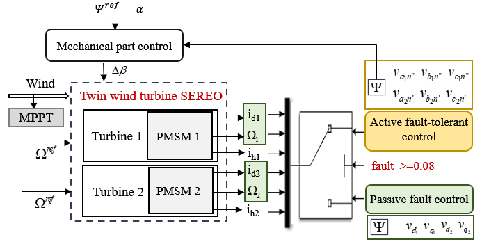
The successive derivatives of the outputs lead to the following equation:
| (24) |
where , with , for .
Note that are the relative degrees of respectively. The vector field and the decoupling matrix , identifying in the appendix, correspond to the successive derivatives of .
Since is a regular matrix, the following
decoupling control based on a new control while respecting homogeneity arguments could be obtained as:
| (25) |
| (26) |
The expressions of , , can be calculated based on [5] and the different homogeneity degrees is given by:
| (27) |
Knowing that , so there is a zero dynamics of dimension 1.
| (28) |
Comparing with [4], the dynamics of zero is even input-to-state stable (input: ) [13]. From equation (28), the dynamic of zero depends on the external input which is not directly influenced by the defect.
The advantage of the active fault-tolerant control, that it use the estimation of the fault. This estimation may be done by many diagnosis methods for example [14], [15]. Nevertheless, estimation of fault is not the topic of this paper.
IV Simulation results and discussion
In the case of a classical control, the voltage references are generated in terms of the -rotating frame [16], [17] and then transformed back into -frame. However, ones the fault occurs only on one phase, the three-phases currents increase and generate an uncontrolled direct current .
In order to stabilize these currents, the gains related to the direct currents and in equation (26) are increased (”robustified”), as it was proposed in [4].
As it can be seen in Fig. 3. and Fig. 4., the fault occurs at the time with the severity of . This recent ”robustification", gives a satisfactory behavior with respect to minor faults but it is not efficient if the defect exceeds (Fig. 5.).


As it was described in section III, more tougher faults can not be consider by classical control. In the next, simulation results of the proposed active fault tolerant control are presented. Based on the fact that an inter-turn short circuit on the stator -phase persists with an important severity (equal to ), it seems necessary to use the -model for the control design.


Figure Fig. 6 shows the three-phase currents of the faulty machine after active fault tolerant control. Despite of asymmetric phases in the PMSM under faulty conditions, the sum of the three-phase currents are equal to zero. This reflects the fact that the direct current and the homo-polar component are controlled to be equal to zero (Fig. 8.).
Thus, from Figures Fig. 9. and Fig. 10, it appears that the angular speed as well as the angle orientation follow their references. These highlight that all control objectives are achieved even if the fault is sever.
V Conclusion
In this paper, it was shown that with respect to asymmetric electrical faults, it is necessary to use the -frame. Consequently, an active fault-tolerant control strategy for a twin wind turbine was proposed in this frame. This control is tested for both healthy and faulty cases, when the presence or not of fault and its severity are well estimated. Simulation results highlight the well founded of the proposed approach.
In future research, an estimation method of the fault based on sparsity assumptions [19] coupled with the proposed active fault-tolerant control will be investigated.
The main problem of active fault-tolerant control based on faults estimation process, is its global stability. Because, even if, the faults estimation process is stable and the active fault-tolerant control is also stable, these do not guarantee that the coupling of both is stable.
References
- [1] André Herskovits, Olivier Laffitte, Philippe Thome, and Alain Tobie. V-shaped, bi-rotor wind generator on a spar floating structure. French Patent WO2014060420 A, 1:2014, 2012.
- [2] Pragasan Pillay and Ramu Krishnan. Modeling of permanent magnet motor drives. IEEE Transactions on industrial electronics, 35(4):537–541, 1988.
- [3] Jian-wei Yang, Man-feng Dou, and Zhi-yong Dai. Modeling and fault diagnosis of interturn short circuit for five-phase permanent magnet synchronous motor. Journal of Electrical and Computer Engineering, 2015, 2015.
- [4] Mariem Makni, Ihab Haidar, Jean-Pierre Barbot, Franck Plestan, Nabih Feki, and Mohamed Slim Abbes. Analysis and control of twin wind turbine subject to asymmetric fault. In 2020 IEEE Conference on Control Technology and Applications (CCTA), pages 1–6. IEEE, 2020.
- [5] Elias Tahoumi, Franck Plestan, Malek Ghanes, and Jean-Pierre Barbot. Robust control schemes based on higher order sliding mode with energy reduction. In 2019 18th European Control Conference (ECC), pages 3109–3113. IEEE, 2019.
- [6] Wei Chen, Steven X Ding, Adel Haghani, Amol Naik, Abdul Qayyum Khan, and Shen Yin. Observer-based fdi schemes for wind turbine benchmark. IFAC Proceedings Volumes, 44(1):7073–7078, 2011.
- [7] Peter Fogh Odgaard, Jakob Stoustrup, and Michel Kinnaert. Fault-tolerant control of wind turbines: A benchmark model. IEEE Transactions on control systems Technology, 21(4):1168– 1182, 2013.
- [8] Xiukun Wei, Michel Verhaegen, and T Van den Engelen. Sensor fault diagnosis of wind turbines for fault tolerant. IFAC Proceedings Volumes, 41(2):3222–3227, 2008.
- [9] Christoffer Sloth, Thomas Esbensen, and Jakob Stoustrup. Robust and fault-tolerant linear parameter-varying control of wind turbines. Mechatronics, 21(4):645–659, 2011.
- [10] Yolanda Vidal, Christian Tutivén, José Rodellar, and Leonardo Acho. Fault diagnosis and fault-tolerant control of wind turbines via a discrete time controller with a disturbance compensator. Energies, 8(5):4300–4316, 2015.
- [11] Ibrahim Guenoune, Franck Plestan, Ali Chermitti, and Carolina Evangelista. Modeling and robust control of a twin wind turbines structure. Control engineering practice, 69:23–35, 2017.
- [12] Ibrahim Guenoune. Commandes non linéaires robustes de systèmes éoliens. PhD thesis, Ecole centrale de Nantes; Université Abou Bekr Belkaid (Tlemcen, Algérie), 2018.
- [13] Hassan Khalil. High-gain observers in nonlinear feedback control. SIAM, 2017.
- [14] Wafa Torki, Jean-Pierre Barbot, Malek Ghanes, and Lassaad Sbita. Sparse recovery diagnosis method applied to hybrid dynamical system: The case of three-phase dc-ac inverter for wind turbine. Open Access Library Journal, 7(9):1–15, 2020.
- [15] Syrine Derbel, Nabih Feki, Florentina Nicolau, Jean Pierre Barbot, Mohamed Slim Abbes, and Mohamed Haddar. Diagnosis methods for mechatronic systems. In International Conference Mechatronics, pages 43–55. Springer, 2019.
- [16] Li Liu. Robust fault detection and diagnosis for permanent magnet synchronous motors. 2006.
- [17] Lukas Otava, Miroslav Graf, and Ludek Buchta. Interior permanent magnet synchronous motor stator winding fault modelling. IFAC-PapersOnLine, 48(4):324–329, 2015.
- [18] Arie Levant. Homogeneity approach to high-order sliding mode design. Automatica, 41(5):823–830, 2005.
- [19]
Syrine Derbel, Florentina Nicolau, Nabih Feki, Jean-Pierre Barbot, Mohamed Slim Abbes, and Mohamed Haddar. Fault diagnosis via a dynamical sparse recovery method and application to a gearbox system. Journal of Vibration and Control, page 1077546320942698, 2020.