Deep Self-Adaptive Hashing for Image RetrievalConference: Proceedings of the 30th ACM International Conference on Information and Knowledge Management; November 1–5, 2021; Virtual Event, QLD, AustraliaProceedings of the 30th ACM International Conference on Information and Knowledge Management (CIKM ’21), November 1–5, 2021, Virtual Event, QLD, AustraliaPrice: 15.00DOI: 10.1145/3459637.3482247ISBN: 978-1-4503-8446-9/21/11CCS: Information systems Novelty in information retrieval
Abstract.
Hashing technology has been widely used in image retrieval due to its computational and storage efficiency. Recently, deep unsupervised hashing methods have attracted increasing attention due to the high cost of human annotations in the real world and the superiority of deep learning technology. However, most deep unsupervised hashing methods usually pre-compute a similarity matrix to model the pairwise relationship in the pre-trained feature space. Then this similarity matrix would be used to guide hash learning, in which most of the data pairs are treated equivalently. The above process is confronted with the following defects: 1) The pre-computed similarity matrix is inalterable and disconnected from the hash learning process, which cannot explore the underlying semantic information. 2) The informative data pairs may be buried by the large number of less-informative data pairs. To solve the aforementioned problems, we propose a Deep Self-Adaptive Hashing (DSAH) model to adaptively capture the semantic information with two special designs: Adaptive Neighbor Discovery (AND) and Pairwise Information Content (PIC). Firstly, we adopt the AND to initially construct a neighborhood-based similarity matrix, and then refine this initial similarity matrix with a novel update strategy to further investigate the semantic structure behind the learned representation. Secondly, we measure the priorities of data pairs with PIC and assign adaptive weights to them, which is relies on the assumption that more dissimilar data pairs contain more discriminative information for hash learning. Extensive experiments on several datasets demonstrate that the above two technologies facilitate the deep hashing model to achieve superior performance.
Keywords:
Image Retrieval; Deep Unsupervised Hashing1. Introduction
With the rapid development of the Internet, the explosive growth of multimedia data poses huge challenges to accurate nearest-neighbor based searching methods. Instead, due to its high efficiency, the approximate nearest neighbor (ANN) (Indyk and Motwani 1998) based search methods have attracted increasing attention. Among them, hashing technologies contribute remarkably to their fast query speed and low storage overhead.
To be specific, hashing techniques can be divided into supervised and unsupervised categories. Supervised hashing (Shen et al. 2015; Shen et al. 2015; Kang et al. 2016; Gui et al. 2017; Jiang and Li 2017; Luo et al. 2018; Chen et al. 2019; Tu et al. 2021; Tu et al. 2020b) methods use the label information to train hashing models, which achieve fine performance. However, the annotations are highly time-consuming and also expensive to collect, which limits these methods in many practical applications. Due to this scenario, unsupervised hashing methods (Salakhutdinov and Hinton 2009; Kong and Li 2012; Gong et al. 2012; He et al. 2013; Wang et al. 2018; He et al. 2019) have drawn a large amount of attention. Many unsupervised hashing methods have been proposed in the past decade, including Spectral Hashing (SH) (Weiss et al. 2009), Hashing with Graphs (AGH) (Liu et al. 2011), Iterative Quantization (ITQ) (Gong et al. 2012), Stochastic Generative Hashing (SGH) (Dai et al. 2017) , etc. The previous unsupervised hashing methods have made progress in this area, however, they normally adopt shallow architectures and severely depend on hand-crafted features (such as SIFT features (Lowe 1999)), which degrade the learning performance.
In recent years, numerous deep learning techniques have been introduced into unsupervised hashing methods (Lin et al. 2016; Li et al. 2017a; Tu et al. 2019) due to their powerful feature representation capability. With the lack of labels, most of the unsupervised deep hashing methods construct a pairwise similarity matrix with pre-trained deep features. For example, Yang et al. 2018 compute the similarity matrix based on the observation that the distribution of the cosine distance for point pairs can be estimated by two half Gaussian distributions. Once the similarity matrix is built, in most of the existing methods, it will be fixed to guide the hash code learning process. However, such a similarity matrix may be unreliable because it is computed with the pre-trained deep features and ignores the semantic information in the downstream retrieval task. To tackle this issue, Shen et al. 2018 employ a straightway by reconstructing a similarity graph with the fine-tuning features through the Gaussian kernel. However, such specific construction schemes mainly focus on the local structure, which limits the model performance, and also, the reconstruction strategy suffers from high computational costs.
In addition, most of the existing methods (Xia et al. 2014; Cao et al. 2016; Deng et al. 2019) ignore the semantic importance of data pairs during their design of the similarity-preserving loss function. As such data pairs are treated equivalently in the learning process. A few of works (Yang et al. 2018; Zhang et al. 2020b; Zhang et al. 2020a; Qin et al. 2020) primitively divide the data pairs into different types like confident or unconfident, they still fail to provide a fine-grained measurement of the importance of different data pairs. The pairs in the same class are still treated equivalently. However, the priority of different data pairs should be different. Intuitively, the dissimilar data pairs might contain more discriminative information, and be more informative for model training. Otherwise, the informative data pairs will be buried by large number of less-informative training pairs and decline hash learning.
To deal with the aforementioned issues, we propose a novel Deep Self-Adaptive Hashing (DSAH) method to adaptively explore the semantic information under training, and provide two innovative components. The pipeline is shown in Figure 1. In particular, to overcome the disadvantage of fixed pre-computed similarity, we adopt an Adaptive Neighbor Discovery (AND) technique, which mines underlying neighbor relationships behind the fine-tuning features gradually during training, and update the initial similarity graph continuously. Further, we introduce an adjustable pairwise weight term Pairwise Information Content (PIC) to distinguish the different importance of data pairs. In this way, the data pairs with more information would gain greater weights and contribute more to model learning. These two techniques enable DSAH to fully explore the semantic information behind the data pairs and learn better hash codes in a self-adaptive manner. The main contributions of this paper can be summarized as follows:
- •
We propose a novel DSAH method to yield better hash codes in a self-adaptive manner with the full exploration of semantic information behind the data pairs.
- •
We propose the AND technique to refine the pre-computed similarity matrix with the fine-tuned representations during the learning process, which can adaptively capture the implicit neighbor relationships and improve the hash learning performance.
- •
We propose the PIC to measure the importance of different data pairs and use it to weigh them during training, where more dissimilar data pairs will be assigned larger weights to augment their discriminative power. These weights are further adaptively updated with the pairwise similarity distribution when the training iterates.
- •
The extensive experiments on several benchmark datasets show that our DSAH is indeed effective and achieves superior performance, which achieves 6.2%, 8.7%, 2.7% improvement over the best baseline on CIFRA-10, FLICKR25K, and NUS-WIDE datasets, respectively.

2. Notation and Problem Definition
Let us introduce some notations for this paper. We use boldface uppercase letters to represent a matrix, in which represents the -th row of , represents the element of which is in the -th row and the -th column. denotes the L2 norm and represents the Frobenius norm. is the indicator function. is the hyperbolic tangent function. is the sign function, which outputs for positive numbers, or otherwise.
| (1) |
Given a dataset contain samples without human annotations, where is the dimension of samples. The goal of hashing is to learn a function that maps the dataset into a set of compact binary hash codes where is the length of codes.
3. Related Work
In this section, we briefly review the traditional shallow hashing methods and recent deep hashing methods. These methods can be divided into supervised and unsupervised categories, and we mainly focus on unsupervised hashing methods.
3.1. Shallow Hashing
Generally, traditional shallow hashing methods can be classified into two categories: data-independent hashing methods and data-dependent methods. Data-independent hashing methods (Gionis et al. 1999; Andoni and Indyk 2006; Kulis and Grauman 2009) typically use random projection to generate binary code. Locally Sensitive Hashing (LSH) (Andoni and Indyk 2006) is a representative data-independent hashing method, which enables similar data to share similar hash codes in Hamming space. However, data-independent hashing methods require longer binary codes to achieve higher accuracy, which also results in higher storage costs. The data-dependent hashing methods (Weiss et al. 2009; Liu et al. 2011; Gong et al. 2012; Dai et al. 2017) have also received increasing attention in recent years, which aim to learn compact and high-quality binary codes from specific data. One of the most classical data-dependent hashing methods is Spectral Hashing (SH) (Weiss et al. 2009), which was developed to learn binary codes by preserving local manifold structures. The objective function of SH can be written as:
| (2) |
where is the similarity weight between and . is the balance parameter. The optimization of Eq. 2 is equivalent to balanced graph partitioning and is an NP-hard problem. SH solves this problem by introducing spectral relaxation, which removes the discrete constraint. The objective function of SH is to binarize the input so that the Hamming distance approximates the Euclidean distance. Generally, the shallow hashing methods usually encode the input images with hand-crafted features (e.g, of ), which is insufficient to characterize the semantic information of data and thus degrade the performance.
3.2. Deep Hashing
Recently, deep hashing methods (Li et al. 2015; Erin Liong et al. 2015; Li et al. 2017b; Qiu et al. 2017; Cao et al. 2017; Liu et al. 2019; Yang et al. 2019) show promising performance compared with the shallow hashing methods. Xia et al. 2014 is one of the earliest works that introduces the deep neural networks into hashing function learning, where the hash codes are learned by minimizing the following loss function
| (3) |
where is the inner product between deep features. is the relaxation of hash codes since it is difficult to directly optimize the discrete variables. Suggested by Cao et al. 2016, cosine similarity might be a better choices to mitigate the diversity of code lengths and improve the performance, which defined as:
| (4) |
where of Eq.3 is the binary pairwise similarity, which is equal to if and are semantically similar, or otherwise.
In supervised cases, is constructed according to labels. But in the unsupervised settings, the labels are unavailable. To tackle this problem, Yang et al. 2018 empirically study the deep feature statistics and estimate two half Gaussian distributions to calculate the similarity. Song et al. 2018 employs the Nearest Neighborhoods (-NN) to compute a binary similarity with pre-trained features. While Zhang et al. 2020b construct a hybrid-similarity matrix in advance. Tu et al. 2020a utilizes the local manifold structure to construct the similarity graph. However, in these methods, the semantic similarity matrix is pre-computed on the original feature space and is separated from the hash learning process. Intuitively, a good similarity representation is beneficial to hashing function learning, and also, hashing function might provide meaningful feedback to similarity representation. Therefore we hope that the similarity matrix and hashing function can be learned simultaneously, which inspires us to design an adaptive similarity updating method rather than reconstructing a similarity structure based on the updated features (Shen et al. 2018). Moreover, the existing similarity-preservation loss function (e.g, Eq.3) usually neglects the priorities between different data pairs in the learning process. Though several works (Cao et al. 2017; Yang et al. 2018; Zhang et al. 2020b; Qin et al. 2020) divide the data pairs into different groups based on their pairwise similarity, these partitions are also pre-defined and fail to capture the fine-grained priority between data pairs since the pairs within the same group are still treated fairly. Thus the informative data pairs may be buried in a large number of uninformative training pairs.
4. Methodology
In this section, we develop our Deep Self-Adaptive Hashing model. The overall architecture of DSAH is illustrated in Figure 1, which contains three modules: Feature Extraction, Adaptive Neighbor Discovery and Pairwise Information Content. We will demonstrate each module in the following section in detail.
4.1. Feature Extraction
We apply the VGG-19 (Simonyan and Zisserman 2014) for hash function learning and denote it as with network parameters . VGG-19 contains five convolutional layers and three fully-connected layers, to make the network suitable for hash learning, we replace the last layers with a fully-connected layer with 1000 hidden units and followed by a hash layer, in which the number of neurons is equal to hash codes length . To resolve the ill-posed gradient of , we adopt the as the activation function of the hash layer and then we get the approximation of hash code as follows:
| (5) |
Once we finish the training process, we can obtain the discrete hash code as follows:
| (6) |
4.2. Adaptive Neighbor Discovery
In this subsection, we propose the AND, which consists of two steps: similarity matrix initialization and updating.
4.2.1. Initialization
Recent works (Song et al. 2018; Yang et al. 2018; Zhang et al. 2020b; Tu et al. 2020a) have shown that the rich semantic structure can be captured via an elaborately designed similarity matrix. In our AND, we construct an initial similarity matrix at the beginning based on -NN.
We first extract deep features from the relu-7 layer of a pre-trained VGG-19 model and then select images with the highest cosine similarity as the neighbors of each image. Then we construct a Low-order similarity matrix as follows:
| (7) |
Notably, we consider that if the neighbors of two images are highly similar, then these two images should also be very similar. Thus we calculate the similarity of two images neighbors using the expression . Then we select the top samples to construct a High-order similarity matrix as:
| (8) |
In order to take full advantage of these two similarity matrices, we define our initial similarity matrix by combining and together, which is based on the assumption that two similar images should not only be similar in feature space but also share similar neighbors.
| (9) |
However, a drawback of is that it is built with the pre-trained features, which might contain noisy data. Ideally, we hope that the similarity maintains consistency with the fine-tuning features, while the reconstruction is time-consuming. Hence, we next propose an efficient updating strategy to refine the .
4.2.2. Updating
AND provides a progressive mechanism for similarity updating. Given a similarity matrix in the -th round (or in beginning), we first use it to update the model parameters . (e.g, Optimizing the in Eq. 3). Next, we measure the pairwise cosine similarity over the training data pairs through Eq.4 and estimate a threshold by
| (10) |
where the and denote the mean and standard derivation of cosine similarity for those data pairs with , which is defined as:
| (11) |
where is equal to , which counts the number of neighbors in . is a hyper-parameter that control the threshold. Finally, we renew the as follows:
| (12) |
Analysis. The AND is motivated by the prediction interval, aiming to design a dynamic criterion Eq.10 based on the global distribution of learned features. The tuition behind Eq.12 is that these dissimilar data pairs with similarity higher than average similarity of similar pair sets could probably be treated as candidate similar data pairs in next epoch, where controls the tolerance, a larger is more serious while a smaller is looser. The reason why we focus on similar pairs instead of dissimilar pairs is that the neighborhoods-based contains only a few similar pairs (). There is still a lot of information (e.g, neighbors) worth mining in a large number of dissimilar pairs, as the model capacity increases, this information would be better distinguished. Therefore, AND is able to adaptively adjust the similarity according to the learned representation, in a progressive mechanism.
4.3. Pairwise Information Content
In PIC, we discuss the priority of different data pairs for model training. Though Eq. 3 provides a scheme to learn hash codes from similarity matrix , it neglects the importance of different data pairs. All the data pairs with their similarities are treated fairly when calculating loss, so that some informative data pairs may be buried in a large number of samples. To tackle this issue, we propose the PIC, which assigns an adaptive weight for each data pair. If a data pair is more important, it will receive a larger weight and contribute more to hashing function learning. So, we define the following loss function:
| (13) |
where is the weight for the data pair which represents the importance of this data pair.
According to the information theory (Shannon 1948), given an event with probability , its information content is defined as the negative log-likelihood:
| (14) |
If an event has a probability 1 of occurring, then its information content is and yields no information. While an event with probability 0, its information content is . Inspired by Eq. 14, we design the following definition:
Definition 4.1.
Given a data pair , we define an event with probability . The indicates that the image is the top-1 retrieval result of the given query image , which is an optimum matching of image retrieval. Based on this, we define the pairwise information content as:
| (15) |
Typically, if an image is the top-1 retrieval result of the query image , then and should be the most similar. Therefore probability can be expressed as a measure of relative similarity between image and image , and we define as
| (16) |
where is a temperature parameter and is the pairwise cosine similarity in Eq. 4.
Analysis. Given a data pair , if is higher, then the information content that the image can be retrieved through the image is lower. (A special case is to use an image to retrieve itself, then should be lowest or close to 0.) On the contrary, retrieving an image via a highly dissimilar query would bring a lot of information. Figure.2 shows an example, given a query image of Dog, if we retrieve a Car, we would be more surprised than retrieving a Cat. So that we have while , where denotes the pairwise similarity. The tuition behind PIC can work is that a data pair contains highly dissimilar images would provide richer distinctive information, so it should be given a larger weight contributing to the hashing learning. The PIC is based on the pairwise similarity distribution , it is adjustable and adaptive. Moreover, our PIC could also be expressed as a kind of pairwise attention mechanism. Particularly, when is equal to constant 1, the importance of data pairs will be the same and the Eq. 13 will degenerate to Eq. 3.

4.4. Objective Function
In addition, to guarantee the quality of learned hash codes, we introduce a loss to minimize the quantization error between the variables and the binary codes . Therefore, the total loss function can be formulated as
| (17) | ||||
4.5. Optimization
Our DSAH consists of two main parts and since the AND is not end-to-end, we separate the optimization process into two alternate steps. First, we fix the similarity matrix and optimize the network parameter by back propagation (BP) with a mini-batch sampling.
| (18) |
where is the learning rate and represents a derivative of .
Second, we fix the and update the similarity matrix according to Eq. 12. Once the model training is completed, we can obtain the discrete hash code through Eq. 6. The detailed algorithm of our proposed DSAH is described in Algorithm 1.
| CIFAR-10 | FLICKR25K | NUS-WIDE | |||||||||||
| Method | Reference | 16 bits | 32 bits | 64 bits | 128 bits | 16 bits | 32 bits | 64 bits | 128 bits | 16 bits | 32 bits | 64 bits | 128 bits |
| LSH+VGG (Andoni and Indyk 2006) | STOC-02 | 0.177 | 0.192 | 0.261 | 0.304 | 0.596 | 0.619 | 0.650 | 0.666 | 0.385 | 0.455 | 0.446 | 0.567 |
| SH+VGG (Weiss et al. 2009) | NeurIPS-09 | 0.254 | 0.248 | 0.229 | 0.293 | 0.661 | 0.608 | 0.606 | 0.614 | 0.508 | 0.449 | 0.441 | 0.505 |
| ITQ+VGG (Gong et al. 2012) | PAMI-13 | 0.269 | 0.295 | 0.316 | 0.350 | 0.709 | 0.696 | 0.684 | 0.720 | 0.519 | 0.576 | 0.598 | 0.651 |
| AGH+VGG (Liu et al. 2011) | ICML-11 | 0.397 | 0.428 | 0.441 | 0.435 | 0.744 | 0.735 | 0.771 | 0.703 | 0.563 | 0.698 | 0.725 | 0.722 |
| SP+VGG (Xia et al. 2015) | CVPR-15 | 0.280 | 0.343 | 0.365 | 0.406 | 0.726 | 0.705 | 0.713 | 0.703 | 0.581 | 0.603 | 0.673 | 0.681 |
| SGH+VGG (Dai et al. 2017) | ICML-17 | 0.286 | 0.320 | 0.347 | 0.395 | 0.608 | 0.657 | 0.693 | 0.689 | 0.463 | 0.588 | 0.638 | 0.670 |
| GH (Su et al. 2018) | NeurIPS-18 | 0.355 | 0.424 | 0.419 | 0.416 | 0.702 | 0.732 | 0.753 | 0.760 | 0.599 | 0.657 | 0.695 | 0.712 |
| SSDH (Yang et al. 2018) | IJCAI-18 | 0.241 | 0.239 | 0.256 | 0.246 | 0.710 | 0.696 | 0.737 | 0.760 | 0.542 | 0.629 | 0.635 | 0.606 |
| BGAN (Song et al. 2018) | AAAI-18 | 0.535 | 0.575 | 0.587 | 0.591 | 0.766 | 0.770 | 0.795 | 0.802 | 0.719 | 0.745 | 0.761 | 0.759 |
| MLS3RDUH (Tu et al. 2020a) | IJCAI-20 | 0.562 | 0.588 | 0.595 | 0.582 | 0.797 | 0.809 | 0.809 | 0.804 | 0.730 | 0.754 | 0.764 | 0.769 |
| TBH (Shen et al. 2020) | CVPR-20 | 0.432 | 0.459 | 0.455 | 0.474 | 0.779 | 0.794 | 0.797 | 0.799 | 0.678 | 0.717 | 0.729 | 0.739 |
| DSAH | Proposed | 0.596 | 0.617 | 0.622 | 0.635 | 0.805 | 0.816 | 0.831 | 0.836 | 0.747 | 0.769 | 0.787 | 0.793 |
5. Experiments
In this section, we conduct experiments on several public benchmark datasets and evaluate our DSAH method. Particularly, we design the experiments to study the following questions:
- •
Q1: Compared with the state-of-the-art unsupervised hashing algorithms, does our DSAH method outperform them?
- •
Q2: How do the components: PIC and AND, affect the performance of DSAH separately? How do they work?
- •
Q3: Is DSAH sensitive to hyper-parameters?
- •
Q4: How about the efficiency of DSAH?
- •
Q5: What is the qualitative result of DSAH?
5.1. Datasets
Following most hashing-based retrieval methods (Song et al. 2018; Deng et al. 2019; Qin et al. 2020), we adopt the following three widely used public benchmark datasets to evaluate the model performance: CIFAR-10, FLICKR25K and NUS-WIDE. The basic information is listed in Table.2, while the setting details be introduced as follows:
| Dataset | CIFAR-10 | FLICKR25K | NUS-WIDE |
| Multi-Label | |||
| # Images | 60,000 | 25,000 | 269,648 |
| # Classes | 10 | 24 | 21 |
| # Train Set | 10,000 | 10,000 | 10,500 |
| # Query Set | 1,000 | 1,000 | 2,100 |
| # Retrieval Set | 59,000 | 24,000 | 267,548 |
CIFAR-10 (Krizhevsky et al. 2009): Followed the setting of (Song et al. 2018), we randomly selected 100 images for each class as the query set, 1,000 in total. Then we used the remaining images as the retrieval set, among them, we randomly selected 1,000 images per class as the training set.
FLICKR25K (Huiskes and Lew 2008): We randomly selected 1000 images as query set and the remaining images were left for retrieval set. In the retrieval set, we randomly chose 10,000 images as the training set.
NUS-WIDE (Chua et al. 2009): According to the setting in (Zhu et al. 2016), we selected 21 most frequent classes from the dataset and each class contains at least 5,000 related images. We randomly selected 2100 images as the query set and the remaining images were used as a retrieval set. We also randomly selected 10,500 images for training.
For the latter two multi-label datasets, if the retrieved image shares at least one label with the query image, it is considered to be associated with the query image.
5.2. Experiment Setup
Metrics: Similar to (Wang et al. 2017; Shen et al. 2018; Yang et al. 2018), we employed four widely used evaluation metrics to evaluate the retrieval performance, including Mean Average Precision (MAP), Precision of the top N retrieved images (Precision@N), Precision curve (Precision Curve), and Precision-Recall curves (PR Curve). For a fair comparison, all the methods used the same training and query sets.
Baseline methods: We compared our method with eleven unsupervised hashing methods, including six shallow hashing methods: LSH (Andoni and Indyk 2006), SH (Weiss et al. 2009), ITQ (Gong et al. 2012), AGH (Liu et al. 2011), SP (Xia et al. 2015), SGH (Dai et al. 2017) and five deep hashing methods: GH (Su et al. 2018), SSDH (Yang et al. 2018), BGAN (Song et al. 2018), MLS3RDUH (Tu et al. 2020a) and TBH (Shen et al. 2020). The parameters and architectures of the compared methods were according to the setting provided by the original papers. For a fair comparison, all shallow hashing methods used 4096-dimensional features generated by the relu7 layer of VGG19 (Simonyan and Zisserman 2014) pre-trained on ImageNet, as same as the deep features used in the five deep hashing methods during their similarity structures construction.
Implementation details: Our DSAH is implemented based on the Tensorflow framework, while all the experiments are conducted on a workstation with an Intel l5-8500 CPU, and an Nvidia GTX2080 GPU. In the initial similarity construction (Sec 4.2.1), the and are set to the same value 500. When training the network, each training image was resized to as input. We set equal to 10 and adopt the adam optimization with learning rate equal to 1e-4, and the batch size was set to 50. The is set to 1, while the is set to {1, 0, 1} for CIFAR-10, FLICKR25K and NUS-WIDE datasets respectively. And the and are set to 3 and 10 respectively.
5.3. Comparison Results and Discussions (Q1)
5.3.1. MAP & Precision
The performance of our DSAH and baseline methods in terms of MAP@5000 are shown in Table. 1. We can observe that our proposed method significantly outperforms other methods on the three datasets. On CIFAR-10, DSAH obtains an increase of 6.1% (16 bits), 4.9% (32 bits), 4.5% (64 bits), 9.1% (128 bits) comparing with the best competitor MLS3RDUH respectively. On FLICKR-25K and NUS-WIDE, DSAH achieves average 8.7% and 2.7% improvement compared to the MLS3RDUH.
In the practical scenarios, we pay more attention to the top retrieval responses. Thus, we further evaluate the performance on the precision of the top-100 for each method. The results are demonstrated in Table. 3, where we display the result of the shortest (16 bits) and longest (128 bits) binary codes. On FLICKR25K, DSAH achieves 1.5% (16 bits) and 2.3% (128 bits) increases comparing with TBH. On NUS-WIDE, DSAH is improved by 1.7% (16 bits) and 2.9% (128 bits) compared to BGAN. Therefore, both the Table.1 and Table.3 demonstrate that DSAH achieves better performance compared to previous unsupervised hashing methods.
| Dataset | CIFAR-10 | FLICKR25K | NUS-WIDE | |||
|---|---|---|---|---|---|---|
| Methods | 16 bits | 128 bits | 16 bits | 128 bits | 16 bits | 128 bits |
| LSH+VGG (Andoni and Indyk 2006) | 0.175 | 0.411 | 0.608 | 0.745 | 0.393 | 0.651 |
| SH+VGG (Weiss et al. 2009) | 0.291 | 0.446 | 0.715 | 0.700 | 0.518 | 0.625 |
| ITQ+VGG (Gong et al. 2012) | 0.283 | 0.458 | 0.760 | 0.818 | 0.545 | 0.739 |
| AGH+VGG (Liu et al. 2011) | 0.444 | 0.617 | 0.794 | 0.877 | 0.572 | 0.794 |
| SP+VGG (Xia et al. 2015) | 0.284 | 0.514 | 0.788 | 0.852 | 0.601 | 0.756 |
| SGH+VGG (Dai et al. 2017) | 0.285 | 0.536 | 0.622 | 0.814 | 0.457 | 0.764 |
| GH (Su et al. 2018) | 0.410 | 0.519 | 0.773 | 0.843 | 0.651 | 0.777 |
| SSDH (Yang et al. 2018) | 0.216 | 0.269 | 0.753 | 0.800 | 0.595 | 0.662 |
| BGAN (Song et al. 2018) | 0.591 | 0.691 | 0.839 | 0.884 | 0.749 | 0.794 |
| MLS3RDUH (Tu et al. 2020a) | 0.618 | 0.677 | 0.851 | 0.868 | 0.748 | 0.791 |
| TBH (Shen et al. 2020) | 0.499 | 0.586 | 0.849 | 0.877 | 0.702 | 0.775 |
| DSAH | 0.616 | 0.691 | 0.862 | 0.897 | 0.762 | 0.817 |
5.3.2. Precision Curve & PR Curve
To further illustrate the effectiveness of DSAH, we display the Precision curve and PR curve of 64 and 128 bits in Figure. 3. The PR Curve Figure.3 (a)(c)(e)(g)(i)(k) clearly displays the precision at different recall values, which is a good representation of overall performance. In general, a larger area under the PR curve indicates better performance. It can be seen that our PR curve covers more areas in most cases, which means that when the precision is equal, the proposed method will recall more related images; when the number of recall related images is equal, the proposed method has higher precision. Thus, DSAH yields a stable and superior performance. Similar to the PR Curve setting, we display the Precision Curves in Figure.3 (b)(d)(f)(h)(j)(l). It can be seen that the precisions of our methods is relatively higher than the precisions of other methods in most cases. which indicates that given a fixed number of retrieval samples, our method can obtain higher precision outperform other methods.
5.4. Ablation Study (Q2)
Since our method consists of two major components: PIC and AND, we further verify their effectiveness.
5.4.1. Effect of PIC
In order to validate the efficiency of PIC, we design the following variants with different in Eq. 13:
- •
PIC0: is equal to constant 1, and it would degenerate to Eq. 3. This could be treated as a baseline.
- •
PIC: is equal to . This is our proposed PIC.
- •
PIC-: is equal to . This could be regarded as an opposite version of our PIC.
We report the experimental results on the three datasets in Figure 4, which are evaluated with MAP@5000. As shown in Figure. 4 (a)-(c), we could observe that: Firstly, compared with baseline PIC0, introducing PIC weights is able to obtain average 8.2%, 1.2%, 2.1% MAP improvements on CIFAR-10, FLICKR25K and NUS-WIDE datasets, respectively. These results indicate that PIC indeed improves the discriminative power of our model. Secondly, the performance degradation of the third PIC- shows that assigning large weights to similar data pairs will degenerate the performance, which indicates that dissimilar data pairs should receive more attention rather than similar data pairs. These results validate the effectiveness of our proposed weighting method PIC.
How PIC works. To further understand PIC, we display the heatmap of pairwise similarity and their PIC weights within a batch size in Figure. 5. It is shown that those data pairs with higher similarity, especially in the diagonal (self-similar), would receive a lower weight after PIC assignment and dissimilar pairs will reach higher weights.


5.4.2. Effect of AND
To reveal the effectiveness of AND, we conduct an experiment to compare the following variants:
We report the results evaluated with MAP@5000 on the three datasets in Figure. 6. By employing the AND, the baseline model can be generally improved, achieving 1.7%, 1.8%, 1.0% average improvements on three datasets, respectively. Furthermore, the performance can be greatly improved by introducing both PIC and AND, resulting in 8.9%, 3.4% and 3.8% average improvements over baseline in three datasets. The above experiments reveal the effectiveness of PIC and AND of DSAH.
How AND works. To better understand the mechanism of AND, we enlarge the round to 10 and record the changing of threshold and the number of neighbors pairs . Also, to monitor the quality of the updated similarity matrix , we compute an indicator matrix , which element is equal to iff data pairs belong to same class, otherwise equal to . Next, we treat AND as a binary classification problem and as ground-truth, and then design a metric to measure the quality of updated matrix , which is inspired by F-score:
where is equal to , denotes the precision of updated similarity matrix . And denotes the recall of , defined as . In Figure. 7. We could see that in each round, additional data pairs are added to the neighbors set, and the number of similar data pairs converges eventually. This is mainly controlled by the increase of the adjustable threshold . Notably, the climbing confirms the effect of AND, which indeed refines the quality of the similarity matrix and leads to the model’s improvement, especially in the first updating.
5.5. Parameter Sensitivity (Q3)
5.5.1. Study of
In Figure. 8 (a), we study the influence of the quantization effect with different over three datasets, where the code length is 64. From this figure, the performance will degrade when is larger than 10. And the recommended value for is 10, which would bring 4.3%, 3.1% and 2.8% MAP improvements in CIFAR-10, FLICKR25K and NUS-WIDE, respectively.
5.5.2. Study of PIC
In Figure. 8 (b), we investigate the influence of hyper-parameter in PIC. It shows that the proposed method is sensitive and deteriorates when . When is larger than 1, the model performance tends to stabilize and slightly decline, and the recommended value for is 1.0.
5.5.3. Study of AND
In Figue. 9, we evaluate the effectiveness of different hyper-parameters in AND on (a) CIFAR-10 and (b) FLICKR25K datasets, where from -1.0 to 1.0 with a step of 0.25 and the maximum is set to 10, the code length is 64. The diagram in Figure. 9(a) indicates that MAP will increase with increases and then converges around 3 on CIFAR-10 dataset, and a large () might be a good choice. On FLICKR25K, it is noteworthy that when is smaller than , a significant increment would happen in the second round. This is due to the increase of similar pairs, but later proved that this threshold was too loose, leading to model degradation.


5.6. Efficiency Analysis (Q4)
In Table.4, we conduct an experiment to compare the training time of different deep methods on CIFAR-10 dataset. The results indicate that DSAH is efficient and only takes nearly one-third time of the fastest baseline SSDH; Also, DSAH achieves significantly performance with only a fifth of MLS3RDUH’s computation time.
| Methods | MAP@5000 | Training Time (h) |
|---|---|---|
| SSDH (Yang et al. 2018) | 0.256 | 3.0 |
| BGAN (Song et al. 2018) | 0.587 | 5.0 |
| MLS3RDUH (Tu et al. 2020a) | 0.595 | 4.8 |
| DSAH | 0.622 | 1.2 |
5.7. Qualitative Result (Q5)
5.7.1. t-SNE visualization
To better understand the manifold structure of learned hashing code, We compare the t-SNE visualization (Maaten and Hinton 2008) of BGAN, MLS3RDUH, and DSAH in Figure. 10, in which the data points within the same colors belong to the same class. It could be visually found that DSAH shows a clearer structure, in which we can find some meaningful clusters. Those scatter points within the same class (color) thus own smaller hamming distances with each other.


5.7.2. Retrieval Result
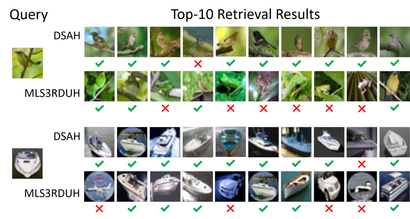
In Figure 11, we display some retrieval examples that return the top-10 samples based on the Hamming ranking distance on the CIFAR-10 dataset (64-bit). Comparing to the best baseline, our DSAH has fewer fault images. Specially, we found that MLS3RDUH confusing birds in a green scene and flags, while the high-quality prediction of DSAH demonstrates that DSAH could well-distinguish the semantic information of images rather than the low-level feature.
6. Conclusions
In this paper, we propose a novel deep unsupervised hashing method DSAH to yield binary codes with fully exploring semantic information behind the data pairs. Particularly, DSAH provides two innovative designs: AND and PIC. To overcome the limitation of fixed semantic similarity, we adopt AND technique to refine the pre-computed similarity matrix with the learned representation and adaptively capture the implicit semantic structure behind the data distribution. Further, we employ PIC to distinguish the different importance of data pairs and assign an adjustable weight to each data pair, which fully explores the discriminative information of training data pairs. By combining PIC and AND in one framework, DSAH learns better hash codes in a self-adaptive manner. The extensive experiments on three benchmarks datasets demonstrate the effectiveness of our techniques, and DSAH can achieve competitive performance.
7. Acknowledgements
This work is jointly supported by the 2021 Tencent Rhino-Bird Research Elite Training Program, and the Major Project of the New Generation of Artificial Intelligence (No. 2018AAA0102900), NSFC under Grant No. 61773268, Natural Science Foundation of SZU (Grant No. 000346).
References
- (1)
- Andoni and Indyk (2006) Alexandr Andoni and Piotr Indyk. 2006. Near-optimal hashing algorithms for approximate nearest neighbor in high dimensions. In 2006 47th annual IEEE symposium on foundations of computer science (FOCS’06). IEEE, 459–468.
- Cao et al. (2016) Yue Cao, Mingsheng Long, Jianmin Wang, Han Zhu, and Qingfu Wen. 2016. Deep quantization network for efficient image retrieval. In Proceedings of the AAAI Conference on Artificial Intelligence, Vol. 30.
- Cao et al. (2017) Zhangjie Cao, Mingsheng Long, Jianmin Wang, and Philip S Yu. 2017. Hashnet: Deep learning to hash by continuation. In Proceedings of the IEEE international conference on computer vision. 5608–5617.
- Chen et al. (2019) Yudong Chen, Zhihui Lai, Yujuan Ding, Kaiyi Lin, and Wai Keung Wong. 2019. Deep supervised hashing with anchor graph. In Proceedings of the IEEE International Conference on Computer Vision. 9796–9804.
- Chua et al. (2009) Tat-Seng Chua, Jinhui Tang, Richang Hong, Haojie Li, Zhiping Luo, and Yantao Zheng. 2009. NUS-WIDE: a real-world web image database from National University of Singapore. In Proceedings of the ACM international conference on image and video retrieval. 1–9.
- Dai et al. (2017) Bo Dai, Ruiqi Guo, Sanjiv Kumar, Niao He, and Le Song. 2017. Stochastic generative hashing. In Proceedings of the 34th International Conference on Machine Learning-Volume 70. 913–922.
- Deng et al. (2019) Cheng Deng, Erkun Yang, Tongliang Liu, Jie Li, Wei Liu, and Dacheng Tao. 2019. Unsupervised semantic-preserving adversarial hashing for image search. IEEE Transactions on Image Processing 28, 8 (2019), 4032–4044.
- Erin Liong et al. (2015) Venice Erin Liong, Jiwen Lu, Gang Wang, Pierre Moulin, and Jie Zhou. 2015. Deep hashing for compact binary codes learning. In Proceedings of the IEEE conference on computer vision and pattern recognition. 2475–2483.
- Gionis et al. (1999) Aristides Gionis, Piotr Indyk, Rajeev Motwani, et al. 1999. Similarity search in high dimensions via hashing. In Vldb, Vol. 99. 518–529.
- Gong et al. (2012) Yunchao Gong, Svetlana Lazebnik, Albert Gordo, and Florent Perronnin. 2012. Iterative quantization: A procrustean approach to learning binary codes for large-scale image retrieval. IEEE transactions on pattern analysis and machine intelligence 35, 12 (2012), 2916–2929.
- Gui et al. (2017) Jie Gui, Tongliang Liu, Zhenan Sun, Dacheng Tao, and Tieniu Tan. 2017. Fast supervised discrete hashing. IEEE transactions on pattern analysis and machine intelligence 40, 2 (2017), 490–496.
- He et al. (2013) Kaiming He, Fang Wen, and Jian Sun. 2013. K-means hashing: An affinity-preserving quantization method for learning binary compact codes. In Proceedings of the IEEE conference on computer vision and pattern recognition. 2938–2945.
- He et al. (2019) Xiangyu He, Peisong Wang, and Jian Cheng. 2019. K-nearest neighbors hashing. In Proceedings of the IEEE Conference on Computer Vision and Pattern Recognition. 2839–2848.
- Huiskes and Lew (2008) Mark J Huiskes and Michael S Lew. 2008. The MIR flickr retrieval evaluation. In Proceedings of the 1st ACM international conference on Multimedia information retrieval. 39–43.
- Indyk and Motwani (1998) Piotr Indyk and Rajeev Motwani. 1998. Approximate nearest neighbors: towards removing the curse of dimensionality. In Proceedings of the thirtieth annual ACM symposium on Theory of computing. 604–613.
- Jiang and Li (2017) Qing-Yuan Jiang and Wu-Jun Li. 2017. Asymmetric deep supervised hashing. arXiv preprint arXiv:1707.08325 (2017).
- Kang et al. (2016) Wang-Cheng Kang, Wu-Jun Li, and Zhi-Hua Zhou. 2016. Column sampling based discrete supervised hashing.. In AAAI. 1230–1236.
- Kong and Li (2012) Weihao Kong and Wu-Jun Li. 2012. Isotropic hashing. In Advances in neural information processing systems. 1646–1654.
- Krizhevsky et al. (2009) Alex Krizhevsky, Geoffrey Hinton, et al. 2009. Learning multiple layers of features from tiny images. (2009).
- Kulis and Grauman (2009) Brian Kulis and Kristen Grauman. 2009. Kernelized locality-sensitive hashing for scalable image search. In 2009 IEEE 12th international conference on computer vision. IEEE, 2130–2137.
- Li et al. (2017b) Qi Li, Zhenan Sun, Ran He, and Tieniu Tan. 2017b. Deep supervised discrete hashing. In Advances in neural information processing systems. 2482–2491.
- Li et al. (2017a) Tong Li, Sheng Gao, and Yajing Xu. 2017a. Deep multi-similarity hashing for multi-label image retrieval. In Proceedings of the 2017 ACM on Conference on Information and Knowledge Management. 2159–2162.
- Li et al. (2015) Wu-Jun Li, Sheng Wang, and Wang-Cheng Kang. 2015. Feature learning based deep supervised hashing with pairwise labels. arXiv preprint arXiv:1511.03855 (2015).
- Lin et al. (2016) Kevin Lin, Jiwen Lu, Chu-Song Chen, and Jie Zhou. 2016. Learning compact binary descriptors with unsupervised deep neural networks. In Proceedings of the IEEE Conference on Computer Vision and Pattern Recognition. 1183–1192.
- Liu et al. (2011) Wei Liu, Jun Wang, Sanjiv Kumar, and Shih-Fu Chang. 2011. Hashing with graphs. In ICML.
- Liu et al. (2019) Xuanwu Liu, Zhao Li, Jun Wang, Guoxian Yu, Carlotta Domenicon, and Xiangliang Zhang. 2019. Cross-modal zero-shot hashing. In 2019 IEEE International Conference on Data Mining (ICDM). IEEE, 449–458.
- Lowe (1999) David G Lowe. 1999. Object recognition from local scale-invariant features. In Proceedings of the seventh IEEE international conference on computer vision, Vol. 2. Ieee, 1150–1157.
- Luo et al. (2018) Xin Luo, Liqiang Nie, Xiangnan He, Ye Wu, Zhen-Duo Chen, and Xin-Shun Xu. 2018. Fast scalable supervised hashing. In The 41st International ACM SIGIR Conference on Research & Development in Information Retrieval. 735–744.
- Maaten and Hinton (2008) Laurens van der Maaten and Geoffrey Hinton. 2008. Visualizing data using t-SNE. Journal of machine learning research 9, Nov (2008), 2579–2605.
- Qin et al. (2020) Qibing Qin, Lei Huang, Zhiqiang Wei, Kezhen Xie, and Wenfeng Zhang. 2020. Unsupervised Deep Multi-Similarity Hashing with Semantic Structure for Image Retrieval. IEEE Transactions on Circuits and Systems for Video Technology (2020).
- Qiu et al. (2017) Zhaofan Qiu, Yingwei Pan, Ting Yao, and Tao Mei. 2017. Deep semantic hashing with generative adversarial networks. In Proceedings of the 40th International ACM SIGIR Conference on Research and Development in Information Retrieval. 225–234.
- Salakhutdinov and Hinton (2009) Ruslan Salakhutdinov and Geoffrey Hinton. 2009. Semantic hashing. International Journal of Approximate Reasoning 50, 7 (2009), 969–978.
- Shannon (1948) Claude E Shannon. 1948. A mathematical theory of communication. The Bell system technical journal 27, 3 (1948), 379–423.
- Shen et al. (2015) Fumin Shen, Chunhua Shen, Wei Liu, and Heng Tao Shen. 2015. Supervised discrete hashing. In Proceedings of the IEEE conference on computer vision and pattern recognition. 37–45.
- Shen et al. (2018) Fumin Shen, Yan Xu, Li Liu, Yang Yang, Zi Huang, and Heng Tao Shen. 2018. Unsupervised deep hashing with similarity-adaptive and discrete optimization. IEEE transactions on pattern analysis and machine intelligence 40, 12 (2018), 3034–3044.
- Shen et al. (2020) Yuming Shen, Jie Qin, Jiaxin Chen, Mengyang Yu, Li Liu, Fan Zhu, Fumin Shen, and Ling Shao. 2020. Auto-Encoding Twin-Bottleneck Hashing. In Proceedings of the IEEE/CVF Conference on Computer Vision and Pattern Recognition. 2818–2827.
- Simonyan and Zisserman (2014) Karen Simonyan and Andrew Zisserman. 2014. Very deep convolutional networks for large-scale image recognition. arXiv preprint arXiv:1409.1556 (2014).
- Song et al. (2018) Jingkuan Song, Tao He, Lianli Gao, Xing Xu, Alan Hanjalic, and Heng Tao Shen. 2018. Binary generative adversarial networks for image retrieval. In Proceedings of the AAAI Conference on Artificial Intelligence, Vol. 32.
- Su et al. (2018) Shupeng Su, Chao Zhang, Kai Han, and Yonghong Tian. 2018. Greedy hash: Towards fast optimization for accurate hash coding in cnn. In Advances in neural information processing systems. 798–807.
- Tu et al. (2019) Rong-Cheng Tu, Xian-Ling Mao, Bo-Si Feng, and Shu-Ying Yu. 2019. Object detection based deep unsupervised hashing. (2019).
- Tu et al. (2021) Rong-Cheng Tu, Xian-Ling Mao, Jia-Nan Guo, Wei Wei, and Heyan Huang. 2021. Partial-Softmax Loss based Deep Hashing. In Proceedings of the Web Conference 2021. 2869–2878.
- Tu et al. (2020b) Rong-Cheng Tu, Xian-Ling Mao, Bing Ma, Yong Hu, Tan Yan, Wei Wei, and Heyan Huang. 2020b. Deep cross-modal hashing with hashing functions and unified hash codes jointly learning. IEEE Transactions on Knowledge and Data Engineering (2020).
- Tu et al. (2020a) Rong-Cheng Tu, Xian-Ling Mao, and Wei Wei. 2020a. MLS3RDUH: Deep Unsupervised Hashing via Manifold based Local Semantic Similarity Structure Reconstructing. In Proceedings of the Twenty-Ninth International Joint Conference on Artificial Intelligence. 3466–3472.
- Wang et al. (2018) Bingning Wang, Kang Liu, and Jun Zhao. 2018. Deep Semantic Hashing with Multi-Adversarial Training. In Proceedings of the 27th ACM International Conference on Information and Knowledge Management. 1453–1462.
- Wang et al. (2017) Jingdong Wang, Ting Zhang, Nicu Sebe, Heng Tao Shen, et al. 2017. A survey on learning to hash. IEEE transactions on pattern analysis and machine intelligence 40, 4 (2017), 769–790.
- Weiss et al. (2009) Yair Weiss, Antonio Torralba, and Rob Fergus. 2009. Spectral hashing. In Advances in neural information processing systems. 1753–1760.
- Xia et al. (2014) Rongkai Xia, Yan Pan, Hanjiang Lai, Cong Liu, and Shuicheng Yan. 2014. Supervised hashing for image retrieval via image representation learning.. In AAAI, Vol. 1. 2.
- Xia et al. (2015) Yan Xia, Kaiming He, Pushmeet Kohli, and Jian Sun. 2015. Sparse Projections for High-Dimensional Binary Codes. In Proceedings of the IEEE Conference on Computer Vision and Pattern Recognition (CVPR).
- Yang et al. (2018) Erkun Yang, Cheng Deng, Tongliang Liu, Wei Liu, and Dacheng Tao. 2018. Semantic structure-based unsupervised deep hashing. In Proceedings of the 27th International Joint Conference on Artificial Intelligence. 1064–1070.
- Yang et al. (2019) Erkun Yang, Tongliang Liu, Cheng Deng, Wei Liu, and Dacheng Tao. 2019. Distillhash: Unsupervised deep hashing by distilling data pairs. In Proceedings of the IEEE Conference on Computer Vision and Pattern Recognition. 2946–2955.
- Zhang et al. (2020a) Haofeng Zhang, Yifan Gu, Yazhou Yao, Zheng Zhang, Li Liu, Jian Zhang, and Ling Shao. 2020a. Deep Unsupervised Self-evolutionary Hashing for Image Retrieval. IEEE Transactions on Multimedia (2020).
- Zhang et al. (2020b) Wanqian Zhang, Dayan Wu, Yu Zhou, Bo Li, Weiping Wang, and Dan Meng. 2020b. Deep Unsupervised Hybrid-similarity Hadamard Hashing. In Proceedings of the 28th ACM International Conference on Multimedia. 3274–3282.
- Zhu et al. (2016) Han Zhu, Mingsheng Long, Jianmin Wang, and Yue Cao. 2016. Deep hashing network for efficient similarity retrieval. In Thirtieth AAAI Conference on Artificial Intelligence.