General relativistic rotational energy extraction from black holes-accretion disk systems
Abstract
The determination of mass and spin parameters of the black holes (BHs) is crucial in the analysis of the merger of BHs and BHs formation and evolution, including accretion. Here we constrain the BH spin with the evaluation of the dimensionless parameter representing the total rotational energy extracted versus the mass of the BH, following procedure introduced in Daly0 that is independent from the details of the specific extraction process. The energy extraction can power an outflow which can be then observed. We relate the energy extraction to the accreting configurations and the accretion processes occurring in a cluster of agglomerate corotating and counter-rotating tori orbiting one central Kerr SMBH, associating to the characteristics of the accretion processes. We relate the regions of tori parameters to features of the energy extraction processes, binding to properties of light surfaces by using the bundles developed in remnant, relating measures in different regions of the spacetimes. We evaluate properties of the BH accretions disks, and correlate spacetimes prior and after their transition due to the energy extraction. Light surfaces are related to the generators of Killing horizons, proving limiting frequency of the stationary observers of the geometries. We consider the photon limiting curves of the stationary observers as constraints for various processes regulated by these frequencies, to relate different BH states, prior and after the energy extraction, investigating regions close to the BH horizons and rotational axis. From methodological view-point we used a naked singularity -BH correspondence defined with metric bundles to predict observational characteristics of the BH–accretion disk system. The analysis points relevant BH spins , and . We show the relation between the rotational law of the tori, the characteristic frequency of the bundle and the relativistic velocity defining the von Zeipel surfaces. The inferior limit on the formation of corotating tori is , for counter-rotating tori ( is the fluids specific angular momentum).
Keywords:
Black holes– Accretion disks–Accretion; Hydrodynamics –Galaxies: active – Galaxies: jetsI Introduction
We examine the extraction of the rotational energy from a Kerr black hole (BH) in the presence of accretion disks. The orbiting accretion matter is considered in the form of aggregates of pressure supported geometrically thick disks of perfect fluids, analyzing purely hydrodynamic models of both tori corotating and counterotating with respect to the central Kerr BH, and centered on the Kerr BH equatorial plane. This model of tori aggregate is known as eRAD, or RAD when the toroidal components are also misaligned with respect to each others and the rotational axis of BHringed; open; dsystem; letter; fi-ringed. Our investigation is centered on the exploitation of a connection between supermassive black holes (SMBHs) and their accretion tori and the states of BHs before and after the process of energy extraction.
The BH rotational energy is supposed to be source of many processes of the high energy astrophysics as the active galactic nuclei (AGN) large-scale outflows Daly0; Daly2; Daly3; GarofaloEvans. The relation between BH spin–disk rotational law, accretion and rotational energy extraction is manifold. The luminosity intensity of the AGNs for example is generally attributed to the fall of gas from the accretion disk on the SMBH, located at the center of the galaxy, therefore en-powering the observed jet emission (see for example recent analysis of the galaxy in the X-band NGC2992 Marinucci, and Mgquasar for a discussion of high-resolution image of the interaction between gas clouds and jets of material ejected from a SMBH at the center of the quasar galaxy MG J0414+0534). However, in different phases of SMBHs evolution cocoons of matter may envelop the hole Gilli2–consequently SMBHs can also be darkened by surrounding material which can be observed on the X-ray band produced by the accreting fluids11 1 For example mission to explore the X-ray emission sector: XMM-Newton X-ray Multi-Mirror Mission)http://sci.esa.int/science-e/www/area/index.cfm?fareaid=23, RXTE (Rossi X-ray Timing Explorer) http://heasarc.gsfc.nasa.gov/docs/xte/xtegof.html or ATHENA http://the-athena-x-ray-observatory.eu/. These plasma concentrations, can show a remarkable variation in their luminosity following the phases of BHs growing – impacting; Ricci. A model of a cluster of misaligned (inclined) tori orbiting a central static SMBH has been developed in the RAD frame in embedded-mnras; embedded-cqg as an orbiting aggregate composed by tori with different inclination angles relative to a central SMBH. The RAD accreting agglomeration can be seen, depending on the tori thickness, as a (multipole) gobules of orbiting matter, with different toroidal spin orientations, covering the embedded central SMBH. BH spin and galactic morphology have been argued to be strongly connected, for example SMBHs in elliptical galaxies possess higher spins than those in spiral galaxies apite1. The spins seem to be related also to the redshift parameter.
In this regard the investigation is increasingly directed to find correlations between different phenomena framed in the BH-disk system: for example in the BH populations and galaxy age correlation and BH–spin shift–accretion disk correlation and in the jet-accretion correlation–see for example Hamb1; Sadowski:2015jaa; Madau(1988); Ricci:2017wmr; Narayan:2013gca; Mewes:2015gma; Morningstar:2014hea; Yu:2015lqj; Volonteri:2002vz; Yoshida; Regan:2017vre; Yang:2017slb; Xie:2017jbz. The BH spin variation follows BH interaction with its environment, therefore many approaches in the evaluation of the BHs parameters and estimation of BH accretion history are connected to the accretion disk physics, based for example on the evaluation of the disk luminosity or accretion rates. It has been shown that the dimensionless spin of a central BH () and the morphological and equilibrium properties of its accreting disks, are strongly related multy. SMBHs spin depends on the angular momentum of the infalling materials tracing back a story of BH accretions in diverse epochs of the BH history LiWangHO. However, an issue of these methods consists also in the fact that the SMBHs spin (with mass of , being solar mass) is strictly correlated with the “mass-problem” and connected with the evaluation of the main features of the accretion processes as the BH accretion rate or the location of the inner edge of the accretion disk. These methods are clearly model dependent Capellupo:2017qpt; McClintock:2006xd; Daly:2008zk, constituting a relevant issue considering that even the definition of the inner edge of an accreting disk is controversial -see for example Krolik:2002ae; BMP98; 2010A&A…521A..15A; Agol:1999dn; Paczynski:2000tz; open; long. On the other hand gravitational waves detection from coalescence of BHs in a binary system may serve, in future, as a further possible method to fix a BH spin parameter Farr:2017uvj; vanPutten:2015eda; vanPutten:2016wpa; 2016PhRvD..93h4042P; 2016ApJ…826…91A.
In this work we consider the approach introduced in Daly0, focused on the definition of SMBH (irriducible) mass function and the definition of rotational energy, and the BH classical thermodynamical law adapted for the analysis of the accretion history of SMBHs in presence of episodic accretion and spin shifts. This approach bridges the BH classical thermodynamic laws with the physical processes, leading to a BH transition through interaction with the surrounding environment.
SMBHs are powerful engines of ejections of matter and energy where the radiative efficiency of energy extraction from rotational energy depends on the spin. In numerous examinations of the energy extraction through the accretion process, the rotational energy converted into radiation corresponds to the binding energy of the fluid, connecting the angular momentum of the accreting material with the radiative efficiency. Furthermore, the SMBHs mass growth rate can be connected with a luminosity function of the host galaxy. Here we consider BHs accreting at (super) Eddington luminosity, and super Eddington accretion disks which are geometrically thick and opaque, pressure supported and cooled by advection–Universe; 2005MPLA…20..561S; 2009CQGra..26u5013S; 2017EPJC…77..860K.
From methodological view-point, we use geometrically thick, "stationary" disks as largely adopted as the initial conditions in the set up for simulations of the GRMHD (magnetohydrodynamic) accretion structures for the numerical analysis–Fragile:2007dk; DeVilliers; Porth:2016rfi; Shafee. The RAD and eRAD models are essentially "constraining-models", providing initial data for dynamical situations. The location of the inner edge of an accreting torus is indeed a key element of the BHs spin estimation, and it is usually identified with marginally stable orbit or with a radius in the region bounded by marginally bounded circular orbit and marginally stable circular orbit according to the accretion disk model, geometrically thick or thin, and the mass of the central attractor. Thick (stationary) disks give a striking good approximation of several aspects of accretion also for more complex dynamical models, estimating the tori elongation on their symmetry plane, the location of the inner edge of quiescent and accreting disks, the location of critical pressure points, an evaluation of the tori thickness, their maximum height.
The inner ringed structure of the eRAD offers a set of interesting scenarios that include its unstable states. More points of accretion can be present in the eRAD inside the ringed structure, which may also include inner shells of jets. Jet in the BH-accretion disk systems can also change the accretion disk inner edge NL2009; Fender:2004aw; Fender:2009re; Soleri:2010fz; Tetarenko18; AGNnoBH; FangMurase2018; 1998NewAR..42..593F; 1998MNRAS.300..573F; 1999MNRAS.304..865F; Fender(2001). In this article we discuss also the correlation between the dimensionless spin of the central BH and the specific angular momentum of the fluid in the orbiting tori, characterizing the system with the rationalized specific angular momenta of the fluid as or , and functions of these variables, supported by considerations related to the general relativistic features typical of the Kerr geometry and describing the rotational law of the eRAD.
The approach introduced in Daly0 for the determination of SMBHs spin, is based on the evaluation of the dimensionless ratio, , of the released energy versus the BH mass, considering the definition of irreducible mass of BH and the BHs thermodynamical laws connecting the BH spin as function of the spin energy and the BH mass. This approach is quite independent from the details of the specific process of energy extraction22 2 Note that the rotation energy extraction process is usually connected with the magnetic fields around the BHs, e.g, the jets are usually connected with the Blandford-Znajek process BZ that could be considered as specific form of the magnetic Penrose process Penrose; Dad2018 that can demonstrate such extraordinary phenomena as acceleration of protons and ions to high energy Universe due to the so called chaotic scattering studied in Stuchlik:2015nlt. Quite recently a new variation of the Penrose process has been presented in cts, that represents new efficient way of extraction of rotational energy related to radiation reaction of charged particles in magnetic fields.. Therefore the quantity , which could be measured eventually as energy released from jet ejection for example, can provide an indication of the lower limit on the BH. The BH spin can be evaluated by the observation of the BH mass and the energy outflowYan-Rong. In the non-isolated SMBHs the outflows, related to the orbiting accretion matter, provide an indication of features of the BH-accretion disks systems. In this scenario a relevant topic is represented by the assumption of counterrotating material which is an intrinsic feature of the eRAD model, as well as the presence of a magnetosphere. This estimation implies the black hole spin changes only due to the BH mass using definition of irreducible mass, grounded on assumption that energy outflow would be powered by the BH rotational energy only Daly:2008zk.
We constrain the BH rotational energy estimating parameters of accretion features in the eRAD frame and the frequencies of light surfaces related to the analysis of many aspects of BHs physics, limits of stationary observers frequencies, connecting measures in different points of spacetime accessible to the observer and points of different space-times before and after the transition induced by the energy release. We use the concept of metric Killing bundles (MBs) introduced in remnant, which are conformal invariant and can be easy read in terms of the light surfaces. Metric Killing bundles define also properties of the local causal structure and thermodynamical properties of BHs as the surface gravity, temperature and luminosityLQG-bundles. Metric bundles can be used to investigate properties of the geometries close to the horizons, connecting the different metrics of the bundles. The observer could extract information (locally) of the region close to the horizons – and connecting different geometries of the metric family considering local properties of causal structure with the analysis of photon-like orbits. Metric bundles of the Kerr geometry are defined as the sets of all Kerr spacetimes having equal limiting light-like (stationary) orbital frequency, which is the asymptotic limiting value for time-like stationary observers (as measured at infinity) and also limits of the tori fluid relativistic velocity. Therefore MBs satisfy the condition , where is a Killing field of the geometry – remnant; observers; ergon; remnant0; remnant1; inprep . The event horizons of a spinning BH are Killing horizons with respect to the Killing field , where is the angular velocity of the horizons. Conditions on constant represents the BH rigid rotation. Characteristic frequencies of the MBs are also the horizons frequencies33 3 In general, a Killing horizon is a light-like hypersurface, generated by the flow of a Killing vector, where the norm of a Killing vector is null. The hypersurface null generators coincide with the orbits of an one-parameter group of isometries, thus there exists a Killing field , which is normal to the null surface.. Metric bundles are defined as curves in an extended plane, , where is the metrics family parameter and is a radial distance. In the extended plane we can consider the horizons confinement and the horizons replicas. For a property of the horizon as distinguished in the extended plane, as the horizon frequency , there is a replica of the horizon, in the same spacetime when there is a orbit (radius) such that , where is a point of the horizon curve in the extended plane. There are horizon replicas in different geometries along the bundle curves, i.e. there is a and a , where and are values of the extended plane parameter , corresponding to two different geometries (distinguished with two horizontal lines of the extended plane) such that: . In both points, , there is equal light-like orbital frequency. The horizon confinement is viceversa interpreted as the presence of a region of the extended plane where MBs are entirely confined-i.e., there are no horizon replicas in any other region of the extended plane, particularly in any other geometry. However this definition is often specified to the confinement of the property in the same geometry. In the Kerr spacetime, this region is upper bounded in the extended plane by the a portion of the horizon curve corresponding to the set of the inner horizon BHs–remnant; remnant0; remnant1; inprep.
In this article we consider phenomenology and processes constrained and regulated by the characteristic frequencies of the bundles. We investigate the extraction of rotational energy in dependence of the accretion features and in relation to the light surfaces through MBs by extrapolating information of the physics close to the BH rotational axis and BHs horizons with the concept of replicas. We predict the possibility of observational evidence of the presence of replicas of the horizon, and indications of the replicas along the bundle curves evident in the thermodynamical transitions of the BH after energy release. We claim that it should be possible to observe the replicas along the axis of the black hole. MBs connect different BH states, prior and after the energy extraction. We consider also the rotational law of the fluid in dependence on the central BH spin.
We note that in more general contexts there can be a different setup on the initial and final state of the BH accretion system, a different outflow contribution and the establishment of special instabilities which can change the BH disks system or even change the BH spin orientation due to Bardeen–Petterson effect, where the BH spin changes under the action of the disk torques-BP75. We base our analysis on the hypothesis that the energy outflow to be measured is powered by the BH spin energy only, however more generally the extracted energy can be determined considering the ratio between the outflow energy versus the spin energy while we consider here the two quantities be coincident. The establishment of runaway instability and the tori self-gravity are also factors neglected in this model that may be relevant, requiring a different characterization of the energy outflow. Furthermore we assume that, from an initial Kerr BH, the final stage of extraction process is a static spherically symmetric Schwarzschild spacetime and we do not consider the contribution of the mass and momentum to the BH subsequent to accretion while geometrically thick disks have large accretion rates (with super Eddington luminosity).
The article plan is as follows: In Sec. (II) we introduce the eRAD model. Sec. (III) focuses on the energy extraction processes: discussion on the energy-spin relations is in Sec. (III.1). Metric bundles, horizon replicas and photon frequencies are the focus of Sec. (III.2). Tori energetics and accretion is discussed in Sec. (III.3). Sec. (IV) contains notes on the RAD and BH-accretion disk spin correlation: the discussion is deepened in Sec. (IV.1), while special sets of tori are introduced in Sec. (IV.2). discussion and concluding remarks follow in Sec. (V). Four Appendix sections close this article: in Sec. (A) and Sec. (B) are some explicit solutions, while in Sec. (C) the relation between Von Zeipel surfaces, metric Killing bundles and tori is investigated and in Sec. (D) an adapted solution parametrization is discussed.
II Fluid configurations on the Kerr spacetime
We consider geometrically thick tori of perfect fluids orbiting a central Kerr SMBH. The metric tensor of the spacetime background can be written in Boyer-Lindquist (BL) coordinates as follows
| (1) | |||
| (2) |
where are the outer and inner Killing horizons respectively, is the outer ergosurface. Here is the (ADM and Komar) mass parameter and the specific angular momentum is given as , where is the total angular momentum of the gravitational source. There is on the planes and is on the equatorial plane . In the region [ (outer ergoregion or simply ergoregion) there is and -Boyer-Lindquist coordinate becomes spacelike. This fact implies that static observers cannot exist inside the ergoregion. For convenience we introduce quantities
| (3) |
where
| (4) |
the lapse function and the frequency of the zero angular momentum fiducial observer (or ZAMOS) observers, whose four velocity is which is orthogonal to the surface of constant . Since the metric is independent of and , the covariant components and of a fluid four–momentum are conserved along its geodesic.


Consequently and are constants of motion for test particle orbits, where is the Killing field representing the stationarity of the Kerr geometry and is the rotational Killing field (the vector becomes spacelike in the ergoregion). It is convenient to introduce also the fluid angular frequency and the fluid specific angular momentum as follows
| (5) |
The case of an orbiting circular or toroidal configuration is defined by the constraint , as we assume the motion on the fixed equatorial plane which is also the plane of symmetry of each toroid of the configurations (), besides no motion is in the angular direction and it is . We mainly consider in our analysis the case of positive values of for corotating and counter-rotating orbits, or for corotating and counter-rotating fluids. Couple of orbiting toroids, , with are said corotating while toroids having are said counterotating. The geodesic structures, composed by the radii regulating the particle dynamics, regulate also large part of the disks dynamics especially in the case of geometrically thick tori, namely the marginally circular orbit for timelike particles , which is also the photon orbit, the marginally bounded orbit is , and the marginally stable circular orbit is for corotating and counter-rotating motion. Radii of geodesic structures are relevant to the accretion physics. We consider also the radius as solution of , and the set of radii and or more generally where
| (6) |
where there is .
Each toroid is described by a one-species particle perfect fluid (simple fluid) energy momentum tensor where
| (7) |
where from the conservation of the energy momentum tensor projected along each fluid four velocity and the related 3-sheet spatial metric tensor projector we obtain the continuity (density evolution) equation and Euler equation for the pressure respectively
| (8) |
where and are the total energy density and pressure as measured by an observer moving with the fluid. Properly chosen boundary conditions determine the inner ringed structure of the tori agglomerate. Then model constructed in ringed; open; dsystem; letter; multy; long; proto-jet; embedded-mnras; embedded-cqg is known as ringed accretion disk (RAD) for tori with a generic inclination with respect the central attractor (aggregates of tilted tori). For the case we consider here, where all tori are centered on the equatorial plane of the attractor the model is distinguished as eRAD, Figs (1). For the symmetries of the problem, we always assume and , being a generic spacetime tensor (we can refer to this assumption as the condition of ideal hydrodynamics of equilibrium). As consequences of this choice, the motion of the fluid is described by the Euler equation only. We assume moreover a barotropic equation of state . From the Euler equation (8) we obtain
| (9) |
where is the effective potential and the function is Paczynski-Wiita (P-W) potential. Assuming the fluid is characterized by the specific angular momentum constant (see also pugtot), we consider the equation for constant obtaining the toroidal configurations as surfaces of constant pressure or constant for , where it is indeed and for . The toroidal surfaces are obtained from the equipotential surfaces, critical points of the effective potential . This set of results is known as von Zeipel solutions.
The function is related to the energy of the test particle as it is . Clearly there is and it is . Models of geometrically thick tori allow the determination of a wide number of aspects of disks morphology, dynamics and stability. The inner and outer edges of an equilibrium torus are also strongly constrained. For each torus, the extrema of the effective potential functions fix the center , as minimum point of the effective potential and the maximum point for the hydrostatic pressure. Cusped equipotential surfaces are associated to tori accreting onto the central BH, due to the Paczynski-Wiita (P-W) hydro-gravitational instability mechanism at the cusp Pac-Wii. More specifically, the matter outflows because of a violation of mechanical equilibrium of the tori, due to an instability in the balance of the gravitational and inertial forces and the pressure gradients in the fluid. The cusp , inner edge of the accreting torus, corresponds to the maximum point of the effective potential and also the zero point for the hydrostatic pressure. The distribution of these critical points, fixing the distribution of tori in the eRAD, as well as features of stability properties, are governed by the RAD rotational law , regulating the distribution of tori in the RAD. Function on the other hand provides the values of at the critical pressure points inside each torus of the agglomerate. Thus the equipressure surfaces at constant, could be closed, determining equilibrium or quiescent configurations, cusped for the "accreting" tori, or also open for proto-jet configurations related to jets open; proto-jet; Koz-Jar-Abr:1978:ASTRA:; Pac-Wii; abrafra, constituting funnels of matter with a cusp on the equatorial plane, characterizing the possible inter-disk activity in the agglomerate, such as the arising of proto-jets shells, collision or double accretion long; open. Each orbiting toroid is governed by the general relativistic hydrodynamic Boyer condition of equilibrium configurations of rotating perfect fluid. Within the so called “Boyer’s condition”, we can determine the boundary of stationary, barotropic, perfect fluid body as the surfaces of constant pressure (also equipotential surfaces) which are also called Boyer surfacesBoy:1965:PCPS:.
We can define the ranges of fluids specific angular momentum governing the fluids and tori topology as follows (we adopt the notation for any quantity evaluated on a radius ):
: for there are quiescent and cusped tori–where . Therefore tori have topologies ; the accretion point is in and the center with maximum pressure in (for tori with ).
: for there are quiescent tori and proto-jets–. Topologies are possible; the unstable point is and center with maximum pressure ; For these configurations there is .
: for there are only quiescent tori – : and center .


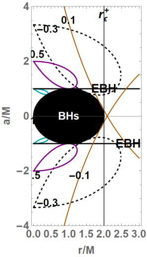
For illustration of the presented definition see Figs (2): left panel shows the open surfaces and the limiting cusped surfaces with cusps at for counterrotating and corotating fluids respectively, enlightening the spatial separations between the two sets of fluids, and the vertical direction parallel to the BH rotational axis. Center and right panels show radii solutions of for corotating and counterrotating tori used in Eq. (6), the separation is the distance between the center of maximum pressure and minimum pressure in the disk (cusp) when the minimum is defined. The distance depends on the BH spin and the rotation orientation of the fluid respect to the central BH (there is and ).
III Energy extraction
In order to look for global characteristics of rotational energy extraction from black holes we have to introduce specific functions of the black hole spin, which will be addressed in Sec. (III.1). It is also convenient to introduce here some notable BH spins:
| (10) | |||
| (11) |
related to the cross of the radii with the , outer ergosurface on the equatorial plane. We proceed in Sec. (III.1) with the analysis of the BH rotational energy in the eRAD context, while we expand the discussion with the inclusion of the metric bundles, and the concept of horizon replicas in Sec. (III.2). This section closes in Sec. (III.3) with an estimation of the mass-flux, the enthalpy-flux and the flux thickness, determined by the geometric properties of spacetime via the torus effective potential.
III.1 The energy-spin relations
We start by considering the spin function :
| (12) |
relating the dimensionless BH spin to the dimensionless ratio representing the total released rotational energy versus BH mass (measured by an observer at infinity, that is where is the irreducible BH mass), assuming a process ending with the total extraction of the rotational energy of the central Kerr BH–Figs (3). (Here and in the following where we do not intend differently, we shall use dimensionless quantities, viceversa where necessary we will make explicit the dependence on the mass.). We can express Eq. (12) in the form
| (13) |
relating directly the energy parameter to the horizons–see Figs (3). However, as there is (here has units of mass ), only solution has to be considered. Considering , solving for we find the eight functions
| (14) |
Note the general solution , for a couple of spins , provides eight functions , four for each spin and according to the four (not related) signs and –see Figs (6). The surface area of the event horizon identifies the BH irreducible (or rest) mass. The total BH mass can be decomposed into the mass , the rotational energy and, eventually, the electromagnetic energy contribution in the Kerr-Newman solution. Therefore there is (here , black hole’s angular momentum, has units of mass as measured in the asymptotical flat region). The maximum rotational energy which can be extracted from the black hole is . A result of Christodolou and Ruffini gives an upper limit on the energy extraction from the Kerr BH, to the rotational energy extraction, assuming a final stage of the process resulting a static Schwarzschild BH CRR. The bottom limit of , at the end of extraction process, has to be . More precisely, considering and the mass and angular momentum of the initial state of the BH, the upper limit for the energy extracted during the stationary process bringing the BH to the state is . All the quantities are evaluated at the state prior the process, therefore all the quantities evaluated here inform on the status of the BH-accretion disk system at its initial state (0), by evaluating the related parameter. The BH angular momentum in the final state is zero. Obtaining the limit of of energy extraction (hence ) where at the state (prior the extraction) there is an extreme Kerr spacetime (having spin ). Eq. (12) has been found considering the rotational (spin) energy , where is the light velocity and is the BH irreducible mass. The rotational energy is equal to the extracted total energy of the outflow .
Consider the state prior the extraction, there is
| (15) |
the variation is thus
| (16) |
( is the frequency of for the outer Killing horizon.). From the first law of thermodynamic , and (extracted rotational) energy emission is essentially44 4 We note that analogue reasoning guides a first evaluation of the energy radiated by gravitational waves following two black holes collisions resulting in a merger. (Particularly considering three Schwarzschild BHs the maximum limit is coincidentally otherwise in case of rotating BHs the maximum values is )55 5 Note that the Smarr formulas can be modified considered an embedded black hole actually an astrophysical not isolated BH immersed in material environment, where there is an additional contribution of the non-vanishing energy–stress tensor due to the matter–see Bardeen in BARDEEN.
| (17) |
In general, there is (dimensionless) and . However, an immediate calculus from definition of rotational energy, , with quantities evaluated at the initial state prior the process leads to the restricted range where , limiting therefore the energy extracted to a superior of of the mass . It is convenient to view in its extended range , and to focus on an extended range corresponding to the outer and inner horizons in the sense explained below. The extension is intended as a reparametrization of the spin , since shows remarkable properties of symmetries. We shall see that this extension does not preserve the symmetry when applied to certain properties of the disk.
As clear from Figs (7), functions and of Eq. (13) are symmetric in . For spin value corresponding to the Scwarzchild spacetime, , there is (note in the extended range , corresponds also to the values and ). Each curves constant corresponds generally to four values , excluding some notable cases as the value and . There is a maximum as function of the spin, (and ) where and (the extreme Kerr BH). Measuring therefore will provide indication of the BH spin. This method, independent of the specific model of energy extraction, was introduced first in Daly0, and applied in other analysis in Daly0; Daly2; Daly3; GarofaloEvans. Here we connect the quantities with the tori parameters and fluid angular velocity .


The analysis using function in Eq. (12) distinguishes continuum curves of classes of attractors in a plane .
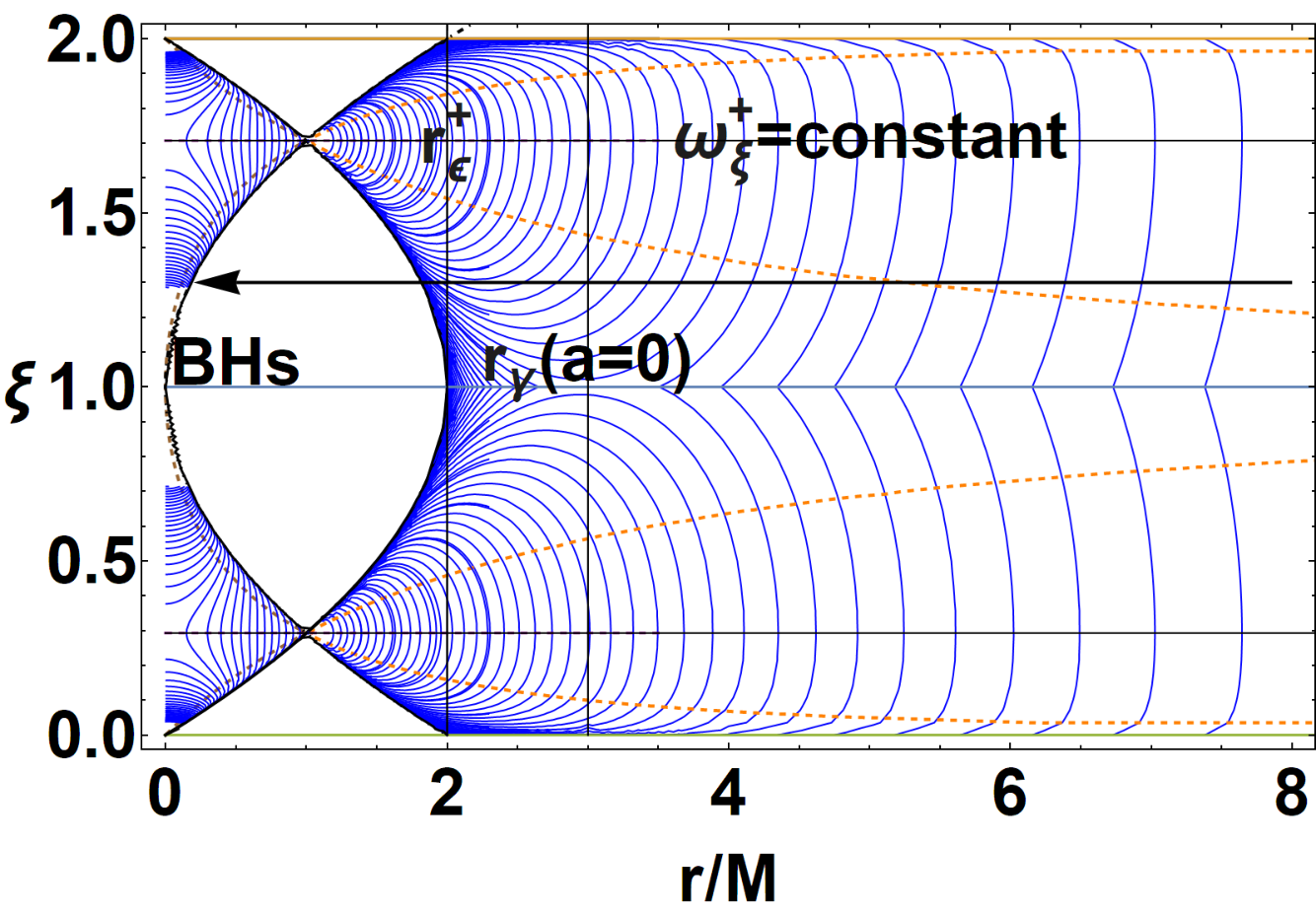
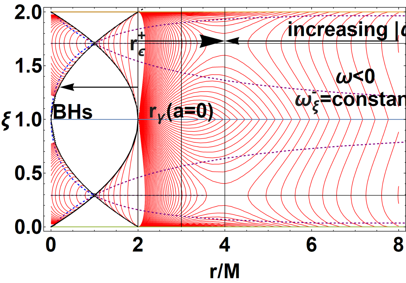
The study of the relativistic velocity of the fluid, constrained by the characteristic frequencies of the metric bundle introduced below, allows to alternatively constrain the tori fluids and to constrain structures dependent on the light surfaces defined by the boundary of stationary observers orbits. The relativistic velocity of the fluid is related to the function of the fluid specific angular momentum and the conditions of von Zeipel, governing the relation between and –(see Eqs (5)–zanotti. Von Zeipel theorem characterizes any stationary, axisymmetric, non-self-gravitating perfect fluids in circular motion in the gravitational field of a central compact object. It guarantees that the angular velocity depends only on the specific angular momentum and the metric components, therefore velocity and parameter have common iso-surfaces (assuming a barotropic equation of state). The von Zeipel theorem eventually represents a set of integrability conditions to compute the equilibrium toroidal solutions. Tori models defined here have four velocity sharing symmetries with the stationary observers, therefore bounded by the limiting relativistic velocities (light-like orbital angular frequencies) of photons defining the light-surfaces regulating many aspects of the BH physics and accretion physics and jet launching or the magnetosphere structure around a BH accretion disk system. Light surfaces are given explicitly in Appendix (B). The connection with the von Zeipel surfaces is explored in Appendix (C). The fluid specific angular momentum is therefore delimited by the the light-like orbital frequencies defining the light surfaces and, as particular case the horizon angular velocity .
The concept of metric bundles introduced here is based on the classes of all the geometries having the same limit frequency in a point; these classes can be represented as curves in a plane called the extended plane, where they are all tangent to the curve defining the Killing horizons of the Kerr geometries. The angular momentum of the fluid and its relativistic velocity are constrained in a point by the frequency values of the intersection of two bundle curves, at fixed plane. There are situations where these frequencies are replicated in other portions of the spacetime (the replicas) thus giving the same constraints. For this reason it is useful to use the concept of "extended plane" introduced in remnant in the definition of metric Killing bundles. Some bundles on the equatorial plane of the Kerr spacetimes are represented in Figs 4. The characteristic frequencies are the limiting photon-like frequencies of the stationary observers , and also the horizons frequency of the BH identified in the extended plane by the tangent point of the bundle with the horizon.
Metric bundles are collections of black holes or black holes and naked singularities (NSs) defined generally for any axially symmetric spacetime with Killing horizons.
Each geometry of the bundles has equal "limiting photon frequency", , which is the characteristic frequency of the metric bundle, and it is also demonstrated be the frequency of a BH Killing horizon as defined in the extended plane . Metric bundles are represented by curves in the extended plane tangent to the horizon curve, which therefore emerges as the envelope surface of all the bundles. The metric bundles introduced in remnant satisfy the conditions defining the null particles frequencies for the vector which is also an horizon frequency for a certain spacetime with spin on the curve in units of mass. (We note that the curves would be featuring counter-rotating orbits.). We deepen this definition below.
III.2 Metric bundles, horizon replicas and photon frequencies
Metric bundles (MBs) of the Kerr geometry were fully characterized in inprep–see also remnant0; remnant1; remnant; LQG-bundles. This definition concentrates on the null orbits frequencies of the stationary observers on the orbits , and introduce the concept of replicas for light-surfaces with equal photon frequencies, which is useful to connect different points of the spacetime, and different geometries following the BH transition for the rotational energy release. More precisely we define the replicas in the extended plane , as a special set of points of the extended plane corresponding to equal (positive) limiting frequency remnant1; remnant0. It is proved that there is a maximum of on the section of the extended plane for fixed plane. In the case considered here, replicas are a couple of orbits (and planes ) corresponding to the same value of the limiting frequency which is also the horizon frequency of the BH defined by the tangency condition of the bundle with the horizon: all the geometries of the bundles have at an point and , one equal limiting frequency (the characteristic bundle frequency). More generally, we can extend the definition of bundle to group geometries on the basis of an equal value of a property , but the convenience of the choice of the orbital limiting frequencies for photon is manifold: this definition is naturally related to the geometry symmetries, it has a numerous of relevant astrophysical applications; eventually, in the extended plane, the BHs horizons emerge as the envelope surface of all the bundle curves, providing therefore also an horizon definition.
The concept of horizon confinement can be introduced by considering that there is a replica when in the same spacetime it is possible to find at least a couple of points having the same value of properties . There is a confinement viceversa, when that value is not replicated. In the Kerr spacetime, part of the inner horizons frequencies are "confined". The confinement analysis, which is a study of curves topology in the extended plane and particularly the self-crossing of the bundle curves in the extended plane, provides the possibility to extract information of determined local properties of the spacetime in some regions, by their possible replicas in other regions more accessible to the observers. Conversely, it provides a way to connect measures in different spacetimes, bundles connect different points in different spacetimes, all characterized by equal value of the property . Therefore MBs connect two or more points in the same spacetime or different spacetimes and one point of the horizon in the extended plane to other points by equal values of the quantity .
In the Kerr geometry we restrict the definition to the BH case, therefore the section of the extended plane or for (the quantity should not be confused with spin function Eq. (12)), and applying the symmetries for corotating and counterrotating fluids, related to the poloidal angle, connecting a point , typically a point of the outer horizon of the BH geometry, to a set of points all characterized by same value of photon orbital frequency of the horizon. It can be proven that in the extended plane , for fixed plane constant, it is possible to connect two points at most through the frequency of the outer horizon (existence of at most a replica of the outer horizon in the same geometry). In the case of the inner horizon the situation is more complex and it is not always possible to find a replica of the horizonremnant. The dependence of the orbit on the poloidal angle , allows a more accurate study of the regions close to the BH rotational axis, revealing interesting observational implicationsremnant. Similarly transformation from the bundles in to has been discussed in remnant1; remnant0. In this context it is clear that is tied to the rotational energy extraction (we also add further notes on this issue in Sec. (IV.1)). The process of energy extraction brings the point on the horizon from to a point on the horizon curve, in the plane , and then a rigid rotation in the sense of remnant, a shift from an horizontal line of the extended plane to another.

Specifying these arguments, we consider the BHs horizons frequencies and the horizons curves in the extended plane respectively on the equatorial plane
| (18) |
see Figs 5,6,19 and Eqs (13) for functions –Figs (3). It is shown the frequency relevant to the bundle structure for each value of . On the equatorial plane, the zero of the bundles define the Schwarzschild static case, in this spacetime the frequency is related to photon orbit .
Let us consider now the tangent curves to the horizons in the extended planes. There are the functions of the frequency
| (19) |
where is the curve of tangent points of the bundles with the horizons, from now on the tangent curve to the horizon, in the extended plane . In this way we represent the extracted energy in terms of characteristic frequency of the bundle and through the tangency condition of the bundle in the extended plane–Figs (6). Tangent can be written in terms of extracted rotational energy as , represented in Figs. (6); we note the limiting value . We introduce the curves and in the extension of the plane for extended values of .


In Figs. (6) we represented the horizons curves of Figs (7) parametrized as in the extended plane, the inner and outer horizons are shown. The limiting null-like particle frequencies of the stationary observes, horizons frequencies as characteristic frequencies of the bundles are on the equatorial plane given by
| (20) |
see– Figs (4). On the equatorial plane, the bundles are expressed in the form
| (21) |
In our case, the bundles in the plane are evaluated, i.e. bundles describe the Schwarzschild BH, the Kerr BHs as well as Kerr NSs. Considering the counter-rotating orbits, as in remnant1, we take into account also . Accordingly, bundles can be given in the extended plane , providing the eight solutions for –see Eq. (13). Horizons replicas on the equatorial plane are
| (22) |


In Figs (5) we note the special role of the photon orbits and marginally bounded orbit for the Schwarzschild spacetime (the limiting case in the extended plane) for each BH spin. Right panel shows a selection of curves, where frequencies for are shown. Considering the notion of replicas, an observer on a point in the BH spacetime with (dimensionless) spin has orbital frequencies limited by the photon orbital frequencies , here of Eqs (20), reachable only in the case of null-particles. On the outer horizon of the BH spacetime there is and the frequency "window" characterizing the stationary observes reduces to circle defining the BH outer horizon. On the other hand, in the case of weak naked singularities as studied in remnant; remnant0; remnant1; 1980BAICz..31..129S, there is a region (of and ) proximate to the singularity where the frequency range bounded by is not null (in this case interpretable as absence of the horizons) but reduced to a minimum. These singularities have peculiar characteristics emerging very clearly as properties of their bundles in the extended plane. Bundles corresponding to these NSs are tangent to a portion of the inner horizon curve which is not confined. This is related to a region in the plane that can be further reduced to a minimal range of frequencies and spins around the central limiting value (a bottleneck) ergon. The issue of naked singularity characterization goes beyond the targets of this analysis, however we can say that such NSs are characterized by this bottleneck regions connected to the horizons as their "remnants" or "memory" of the BHs horizons in the extended planeremnant. This region coincides with the region where repulsive gravity effects appear. NSs region of the extended plane containing parts of the MBs tangent to the horizons have a role in the MBs analysis of BHs as the origins of the bundles, which are points of the axis also in NSs.
Replicas connect the two null vectors and (we also consider the special case ), i.e., defining the bundles and connecting points belonging to in the same spacetime or different spacetimes. Here we consider the observers registering the presence of a replica at the point of the BH spacetime with spin , belonging to the Killing bundle . The observer will find the replica of the BH horizon frequency at point , therefore her/his orbital stationary frequency will be where one of () is the horizon frequency, i.e. the horizons frequency is replicated on a pair of orbits , the second light-like frequency is the frequency of a horizon in a BH spacetime which is correlated by the bundles to in the considered spacetime. The relation between the two frequencies is determined by a characteristic ratio studied in details in remnant.
In the extended plane, , the extracted rotational energy is see Figs (3). Clearly, the extended plane does not describe bundles, or portions of bundles , in the NSs region similarly to the plane , particularly in the case fully contained in NS region which is defined by the frequency , corresponding to the Kerr extreme BH as tangent point bundle-horizon66 6 Exploring the role of the NSs as considered in the extended plane, we note that the three solutions not verifying the condition could provide an indication of the portion of the bundles contained in the NSs region. We note that considering the characteristic frequency of the bundle on the equatorial plane tangent to the curve of the outer horizon in the extended plane, thus, , there is a replica in the spacetime at , not shown however in the plane –as clear from Figs (8). It is also evident that these bundle structures are very similar to those obtained for the Schwarzschild case.. Thus it cannot describe energy extraction from a NS although we use a NS to construct the bundles on the BH region.
Function links the former state spin to the rotational energy extraction in the subsequent phase where the BH is settled in a Schwarzschild BH. Therefore analysis of a quantity relates quantities , before the transition, to the energy extraction measured by – Figs (8)–Camezin; Punsly; Meier.
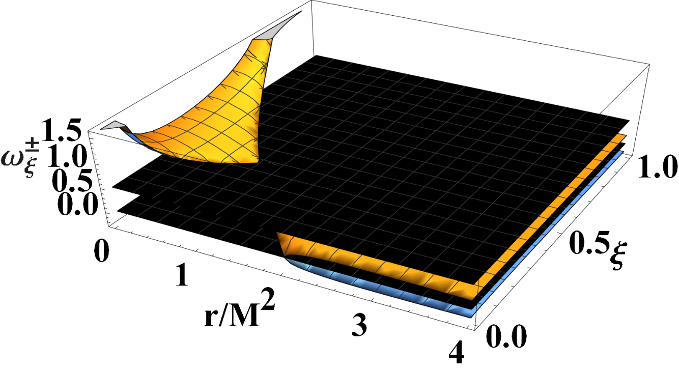
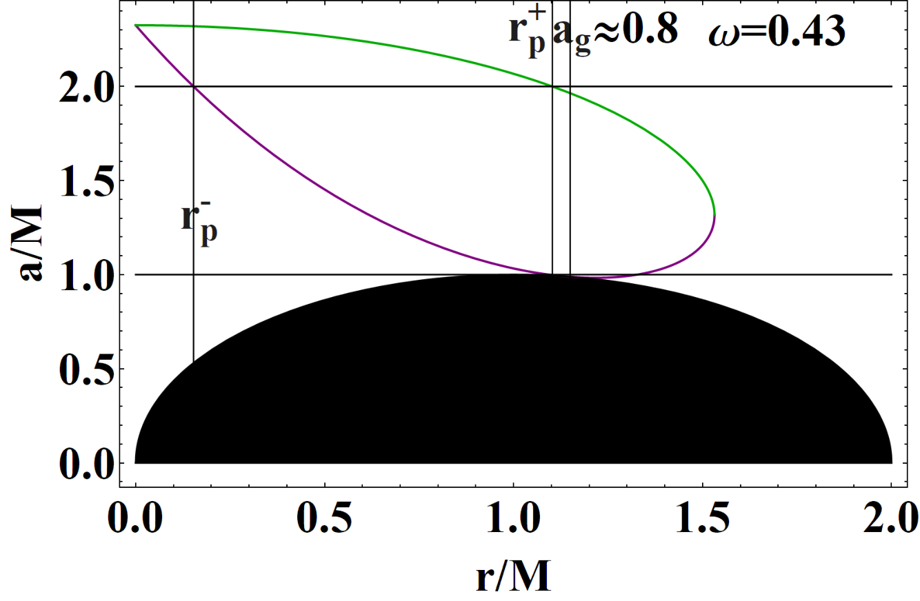
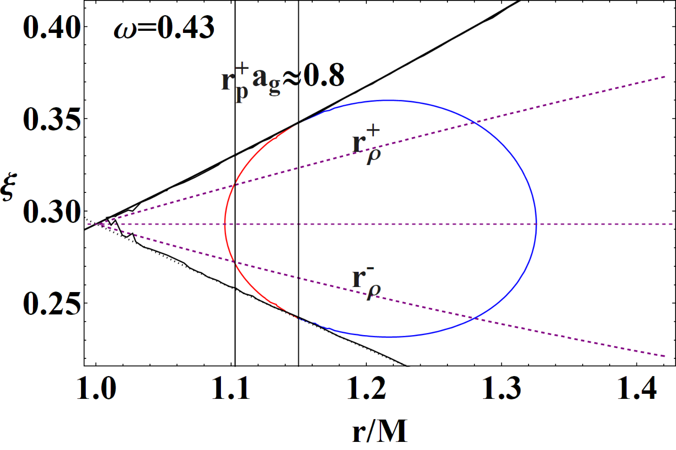
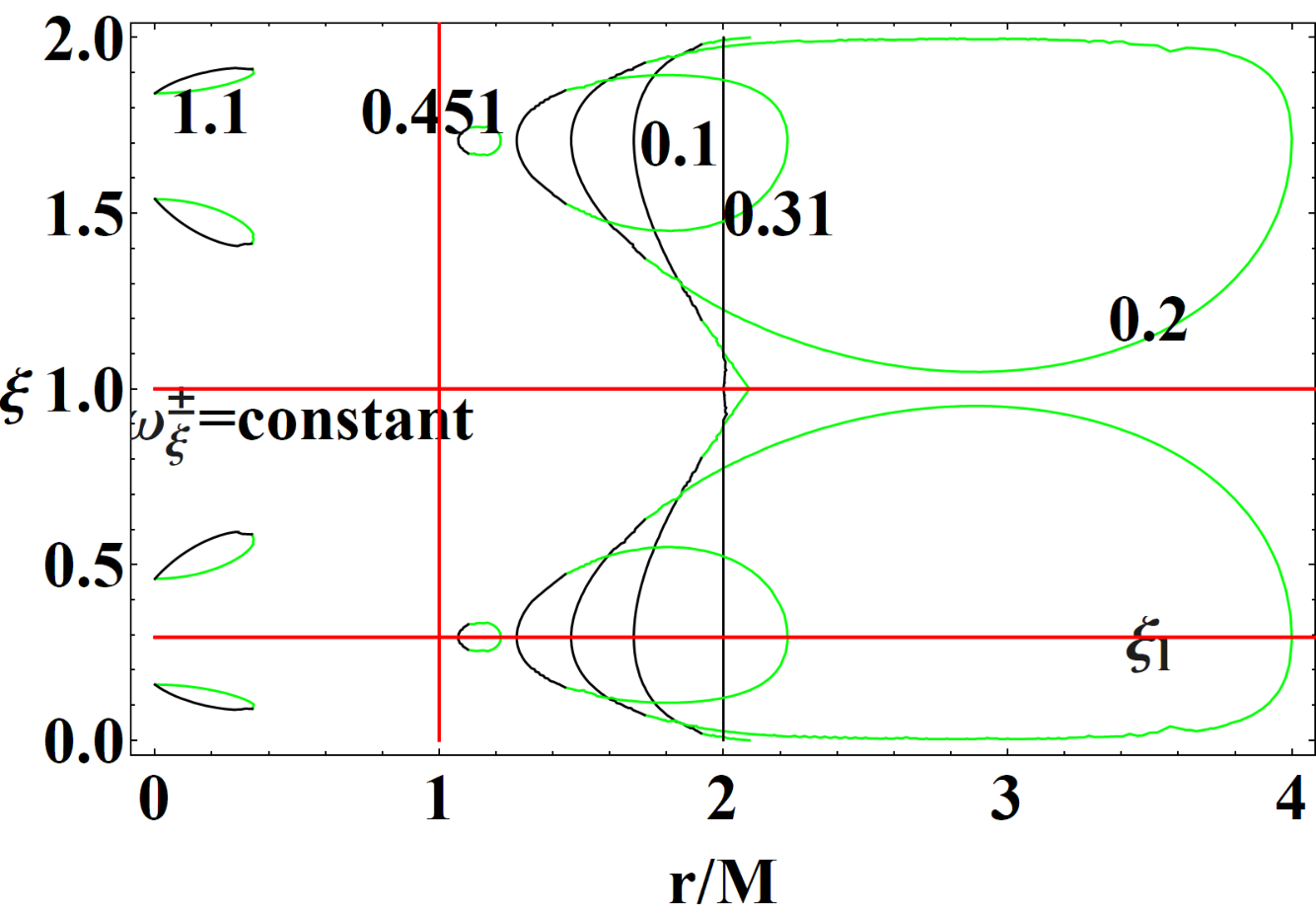
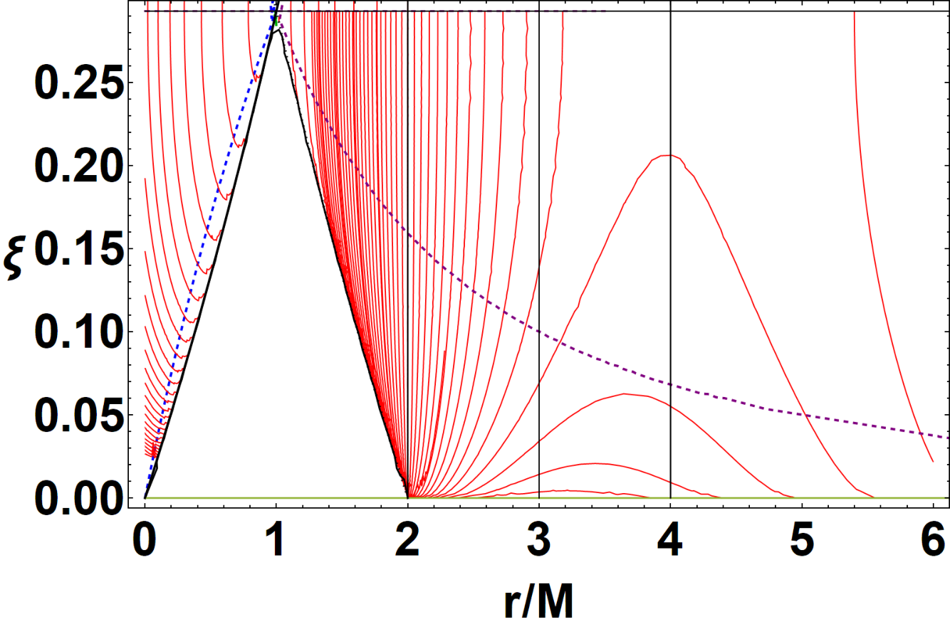
In the processes of accretion and classical interaction between BHs and the surrounding matter and fields, the horizon area, , can remain constant or can increase. Assuming that all the (corotating) fluid provides an initial contribution through the cusp , from its specific angular momentum and a specific internal energy, the mass and angular momentum of the BH grow by the corresponding amount given by , and (). Next section focuses on the analysis of quantities relative to the disks as functions of the extracted energy measured by the observers. In Figs (9) we represent the geodesic structure as functions of the rotational energy parameter, including the curves constant which define each torus of the RAD agglomeration as functions of the extracted rotational energy in the range and for corotating and counter-rotating fluids. The ranges defined by values , and define the topology of the critical configurations. In Figs (10) the curves are shown as functions of providing the values of the parameter of each toroidal configuration (at constant) at the critical points of pressure inside the configurations. (Note that the functions in Figs (10) are not symmetric in the left and right range of the extreme value ) Therefore, in this frame we solve equation obtaining the curves:
| (23) |
representing the families of tori-BHs systems. Note that solutions of or provide the solutions of Eq (23), for where is positive or negative, if fluids are corotating or counter-rotating. (Alternatively solutions are given in Sec. (A).) Considering the geodesic structure in the extended plane, we can find classes of spin-radius
| (24) |
connecting the geodesic structures of different spins of the Kerr BHs, where refers to the photon orbits , and refers to the horizons. Similar definitions can be used for , showed in Figs (9).


Explicit solutions in different parameterizations are in Sec. (A). Solving the problem , we find functions connecting the tori, defined by values , and locations of maximum and minimum pressure points , with the rotational energy , which now can be read in the extended plane. Figs (13) and Figs (14) show the results of for corotating and counter-rotating tori and the location of the inner edge of accretion tori as function of the rotational energy . In Figs (2) we give the spread between the rotational law curves which demonstrates the ranges of parameters for the existence of tori, tori extension on the equatorial plane and maximum possible distance between tori in the eRAD. We relate in this way centers and cusps (in general critical points) of family of tori for different black holes, determined as solutions of the problem on the rotational curve of the eRAD. The distance relates the point of maximum and minimum pressure inside each torus, enlightening the outstretching of the torus on its equatorial plane and the location of the inner edge (cusp).
The parameter on the horizon at the extreme case where the frequency is and . The characteristic frequencies of the bundles, seen as horizons frequencies in the extended plane, are
| (25) |
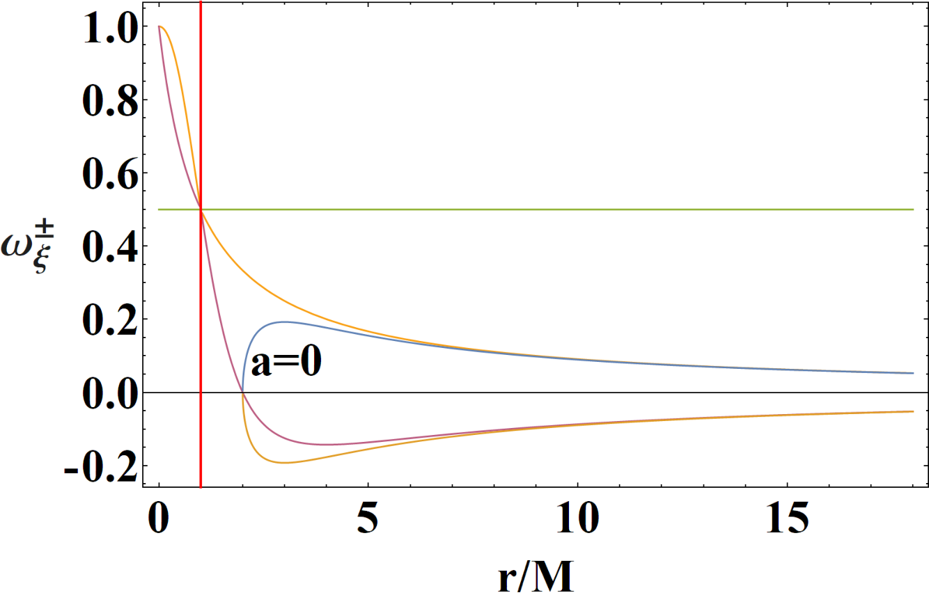
has a saddle point for the extraction parameter correspondent to the spin and frequency )—-see Figs (11) and Sec. (IV.1). (The spin , corresponds to a BH with and BH with spin to .)
III.3 Energetics and accretion
Our analysis focuses on a state prior the extraction process, considering the RAD tori of polytropic fluids, with pressure given by polytropic equation of state , here is a polytropic constant, is the polytropic index. The limiting case of polytropic index would correspond to the case of zero pressure represented by gravitating dust of test particles. We estimate the mass-flux, the enthalpy-flux (which is related to the temperature parameter), and the flux thickness, which are important for the evaluation of the energy release from RADs–see abrafra; Japan. In details, definitions of these quantities are listed in Table (1).
| Quantities | |
|---|---|
All these quantities can be written in general form , and , considering that is the Keplerian frequency of the accreting tori cusp (the inner edge of accreting disk), where are functions of the polytropic index for each torus. Parameters within the constraints constant, fix a polytropic-family, while is related to thickness of the accreting matter flow and the potential , thus denotes, for a torus with fixed specific angular momentum , the (constant) value of the potential of the constant surface corresponding to radius (). We consider also the quantity , where is a limiting case corresponding to a large centrifugal component of the disk tending to balance the gravity and pressure force components in the torus. In this case the inner edge of the accreting tori , there is . In our analysis, for this first evaluation, we define the accretion point and as in Figs (13) (there is therefore ). As the cusp approaches the limiting radius , the potential , which is also the limiting asymptotic value for very large as well as for the emergence of the proto-jets for . The couple of parameters has been fixed, to simplify the comparison of the and quantities in the corotating and counter-rotating tori, and to characterize the dependence of these quantities on the SMBH spin-to mass ratio .
We examine the fraction of energy produced inside the flow and not radiated through the surface but swallowed by central SMBH, the efficiency , together with the total luminosity , the total accretion rate, , and accretion for a stationary flow, . We examine also -quantities–Figs (10,12,13) , for , with the new variables independent from details of the selected specific polytrope, for -quantities and for -quantities. Considering therefore the rate of the thermal-energy carried at the cusp and the disk accretion rate , as well as the mass flow rate through the cusp (i.e., mass loss accretion rate).


The eRAD is in fact a geometrically thin disk with a complex inner ringed structure composed by both corotating and counter-rotating geometrically thick accretion disks having many features common with the thick and opaque disks as the expected super Eddington luminosity. This evaluation, leading to the results shown in Figs (12), connects diverse states of the BH and its RAD system, more specifically, different initial states , prior the rotational energy extraction. The procedure is based on the geometric considerations derived from the geometrically thick torus model considered here: each RAD component is pressure supported and subjected to conditions of the von Zeipel theorem, ensuring the integrability of the Euler equation and assumptions on the boundary conditions (which are assumptions on the pressure at the center, point of the maximum pressure, and torus edge, equipressure surface). We limited the description of the situation of BH, neglecting the contribution of mass feeding processes, leading likely to a multi-stage evaluation, as an interactive process may be engaged between geometry and disk similar to the runaway instability. For corotating and counter-rotating fluid characteristics, fluid momenta and location of cusps have different role for energy extraction parameter . For corotating tori the variation of the location of the minimum points of the pressure, the instability points of the toroidal configurations, changes minimally with respect to counter-rotating tori with the parameter . A relevant aspect concerning accretion is whether the presence of double accretion phase due to the doubled inner ringed structure of the RAD, enhances BH accretion, considering also the possibility of interrupted phase of accretion due to the inner screening torus of the couple. There is the maximum of two accreting tori in the eRAD, with the outer torus being counter-rotating, and inner torus, being corotating. This scenario is then enriched by the possibility of inter disk emission jets and obscuring tori, which are typical aspects of the RAD presence around the central SMBH, and shells of jets. The processes related to counter-rotating fluids may however be drastically different from the corotating case especially due to the influence of the ergosurface. There are indeed corotating solutions in the ergoregion for these tori stretching with the inner quiescent or cusped tori down to very close vicinity of the horizons for large BH spinsnext. This is essentially due to the fact that the fluid in the tori could be considered stationary in the sense that the fluid four velocity is , where is the relativistic angular momentum. On the other hand, a cusped (corotating) torus can stretch towards the horizon enhancing the so called runaway instability– see Figs (18).


We conclude from Figs (13) that the functions are not symmetric in the left and right range of the limiting value , we note the different behaviour of the curves for corotating and counterrotating fluids.
IV On the RAD and BH spin–accretion disk correlation
We conclude this analysis exploring tori characteristics in terms of dimensionless BH spin. Here we investigate in detail the dependence of the RAD rotational law and the BH spin. It was proved in dsystem; letter; multy that there is a relation between the specific angular momentum of the fluid of the inner and outer torus of an eRAD couple and the central BH spin , different for corotating and counter-rotating couples. We investigate a simple correlation within the limits of the range of values of the dimensionless spin of the BH ( is the BH ADM mass) and the fluid specific angular momentum , here used to parameterize the torus of the orbiting aggregate, through the value assumed along the distribution curve (the eRAD rotational law) at the point of maximum density and pressure inside each toroidal configuration of the agglomeration. Arguments in support of the existence of such correlation in the form of superior and inferior boundaries of the range, have been discussed in pugtot; multy, while in ergon discussion on the possible geometrical origin of this limit has been highlighted. In this section we resume this topic considering the ergoregion as stationary (corotating) disk solution can also be considered for sufficiently large values of the central BH spin. Therefore, the model is also studied in the regions close to the static limit
Function is considered as a possible reference distribution on the fluid angular momentum in an extended region of any ("fast" rotating) accretion disk. The condition of almost spherical accretion provides a first limit on the rotational law of the fluid in the accretion disk. Sometimes this limit is know as "Bondi regime". Thick disks considered in this article are regulated by a significant centrifugal force which is more generally assumed superior or equal the Keplerian specific angular momentum . In this sense the "slow rotation" case is referred to as "Bondi flows" (being the limit of free fall accretion disks) Bondi. In these (quasi)spherical "Bondi" accretion conditions, the angular momentum is not relevant in the dynamical forces balance, i.e., the (specific) angular momentum in the disk is smaller than the Keplerian one. On the other hand, an accretion disk must have an extended region where matter has a large centrifugal component ()–abrafra. It will be convenient to analyze the accretion disk properties in terms of the ratio or as an important parameter for these models77 7 As discussed in Sec. (II) there are closed toroidal configurations for and . However in pugtot orbiting stationary configurations for different values of and have been constructed. At lower momentum (in magnitude) there are closed surfaces very close to the outer horizon, and related to the inner Roche lobe of the closed tori. The stability of these configurations which have not cusp has however still to be assessed pugtot.
IV.1 On the RAD rotational law , torus specific angular momentum and BH spin .
In proto-jet; pugtot, variables and have been considered to construct the accreting tori around a Kerr SMBH. Many properties of the fluid effective potential are determined by the quantity where there are the limiting values and ( being off function of the polar angle ). The origin of this quantity can be understood by considering the following fact. For simplicity we use here all dimensionless quantities, we introduce the rotational version of the Killing vectors and , i.e., the canonical vector fields and .
Then the contraction of the geodesic four-velocity with leads to the (non-conserved) quantity , function of the conserved quantities , the spacetime parameter and the polar coordinate ; on the equatorial plane it then reduces on . We note the existence of two limiting values related to two bundles frequencies and limiting momenta: and . When we consider the principal null congruence, , the angular momentum that is (and , in proper unit), every principal null geodesic is then characterized by88 8 Here we consider the quantity ; then if we have and therefore for there is . .


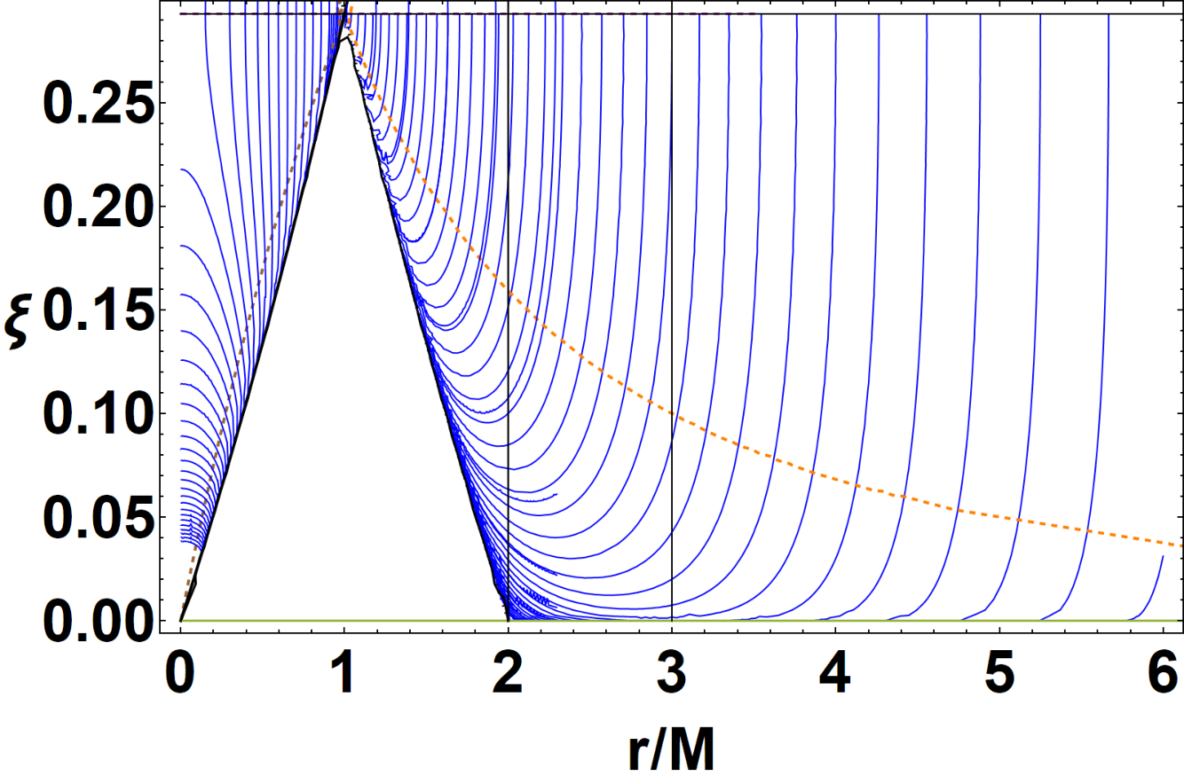
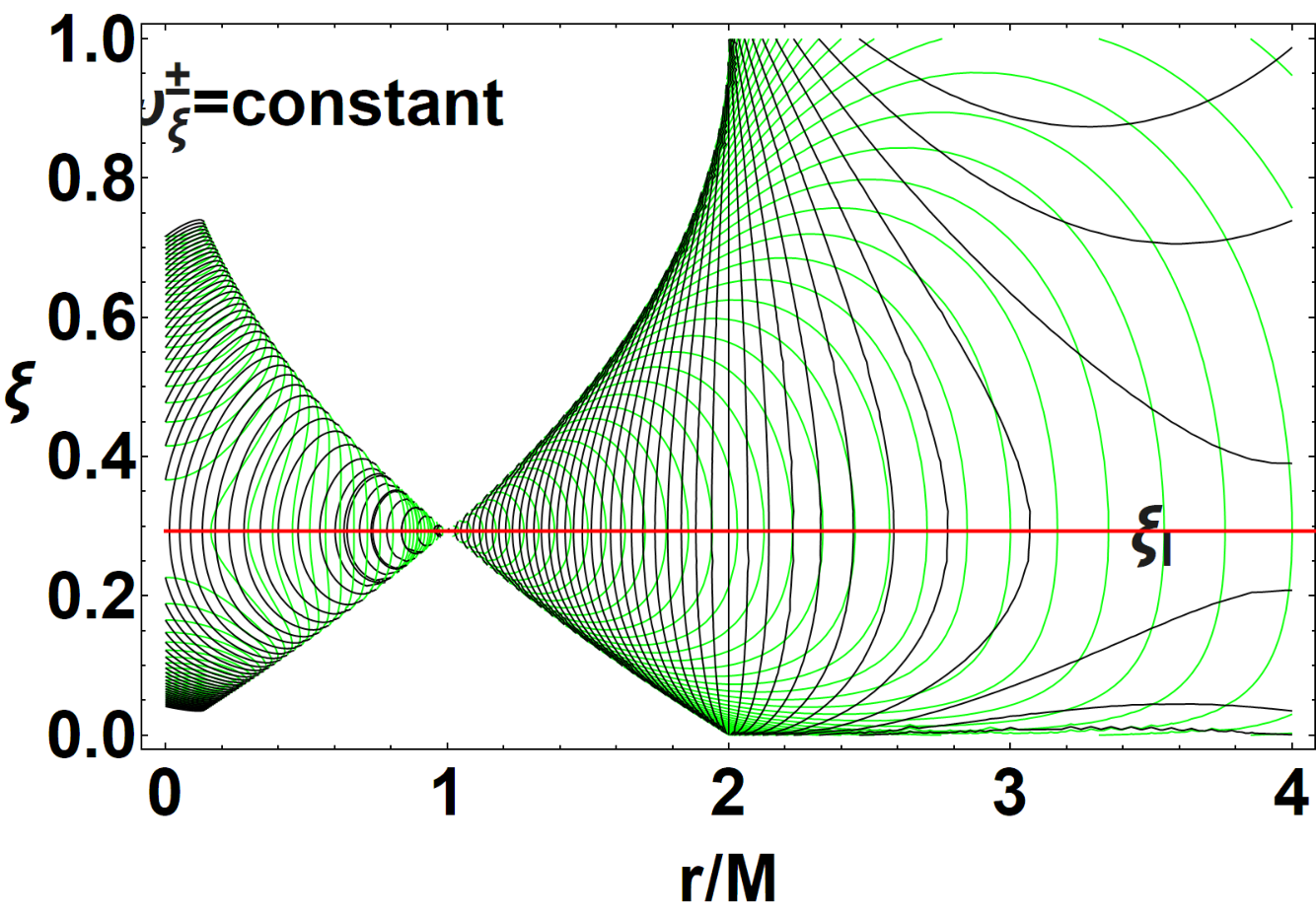
With reference to Figs (15) we considered the "bundles-like" solutions with Killing vector with . We note that these particular bundles solutions appear tangent to the horizon curve in the extended plane . The study of these special solutions is relevant considering the following relations hold: there is where is the origin of the bundles that is at constant in the extended plane , the origin is at remnant; remnant0; remnant1. It is worth noting that in the extended plane at fixed spacetime (an horizontal line), on a fixed plane these curves are bundles at constant frequency. Eventually, we can evaluate the gradient of constant. The following relations also hold: , thus , is the outer horizon frequency in the extended plane. Therefore, featuring an adapted process in terms of the variation of the moment of the BH, there is , which is expression of the condition (here has using of mass square). Note that there is the limit independently from in the spherically symmetric Schwarzschild spacetime. Condition has no solution, but there is the singular surface of the ergosurfaces, , in the extended plane as reported in Figs (15). The condition is realized only at the origin , particularly for there is (then ).
On the other hand, considering the coincidence condition with the horizon curves, the condition for the bundles is solved for which, evaluated on the horizons , gives respectively . The condition implies . The tangency condition of the metric bundles are given in remnant with curve for . The solution of the condition for the frequency is . The horizon curve is clearly delineated as an asymptotic limit of the bundles.
The characteristic frequencies of the bundles, seen as horizons frequencies, are the functions of Eq. (25). has a saddle point for , correspondent to the spin and frequencies )—-see Figs (11). The maximum extractable energy , confirming the relation –see Figs (11). The two bundles whose tangent spin on the equatorial plane is , are tangent to the horizon curve in the extended plane on , with characteristic frequencies and origin dimensionless spins in the naked singularity regions, respectively on the equatorial plane. Obtaining the limit of in the static case , the bundle frequencies have an extreme as function of for the orbit of photon where .
Spin is solution of where . Another relevant spin is which solves the problem for and where , a second saddle point is , where –remnant0.
A different adapted solution parameterizations is discussed in Appendix (D).
IV.2 Sets of tori
An example of distributions of momenta and radius as functions of the spin in the considered parametrization is shown in Figs (17,18). In Fig. (2) we show the dispersion in the corotating and counter-rotating distribution of tori in the RAD.
Considering the situation on the equatorial plane , there are lower bounds in magnitude of the rationalized momentum . It is easy to see that this limit is always given as inferior limit (in magnitude) of the extreme rotating BH case. Therefore, corotating fluid configurations are formed for , where the limiting value increases with decreasing spin. In the counter-rotating case, fluid configurations can form with . The detailed situation is shown in Figs (16), which considers also the limits for the formation of stationary configurations in the ergoregion. For the formation of counter-rotating accreting tori and proto-jets there are the limiting ratios , and . In pugtot it was shown that the limiting cases do not admit any toroidal Boyer configurations, .
A more accurate description is therefore shown in Figs (18), curves of =constant show one torus evolution. The analysis points out two relevant spins: the first at , clear also from the Figure (17), and a second relevant spin is . The crossing of areas and curves show the regions of RAD tori parameter where collision is more probable to occur. This behavior has also a role in the density seeds formation. Considering different regions of the parameters, the separation (corotating-counter-rotating) is larger for the accretion than the proto-jets parameter space, indicating that at high fluid specific angular momentum the corotating and counter-rotating fluids may have not been differentiated in the formation of the early phases of jets, and the separation remains in the range from to independently from the spin. The model reveals also the possibility of jet shells of corotating or counter-rotating fluids.


A detailed analysis points out the following spins :
| (26) |
There is a discriminating value in two spin classes, determined by the value , see Figs (17) dsystem; multy We distinguish the set of spins defined by the cross of the radii of the corotating and counterrotating geodetic structures, and the spins defined by the cross of the corotating and counterotating fluid angular momentum curves as functions of the BH dimensionless spin. Spins regulate the eRAD inner structure associated to classes of SMBHs defined according to their spins. This can be seen by considering the role of the geodetic structures in the torus model construction, fixing location of maximum and minimum of pressure in the torus, respectively the center and inner edge of the torus, and the related orbital regions shown in Figs (17). The inner eRAD structure is defined by the number of tori, their locations and relative rotation, if corotating or counterrotating with the central BH, and their topology. Spins define regions of the rationalized specific angular momentum, , for corotating and counterrotating fuids, regulating also condition on the colliding tori multy; long. Furthermore, in Figs (17) a quasilinear relation as function of is shown, in logarithm scale: where and are constant, and it can be explained by an analysis for small dimensionless spin . It is clear from Figs (9) how the functions of the rotational energy parameter determining the inner structure of the eRAD in terms of the relative location of corotating or counterrotating tori, is more articulated for small , that is for geometries .
On the equatorial plane, the frequency has an extreme for where . In Figs (16) we represent the ratio and the increment , for and denoting geodetic limiting orbits. The differences provide a first indication on the construction of the couples of counter-rotating orbits and therefore the possibility of formation and evolution under spin transition, remaining almost constant for .


Curve representing classes of torus/attractor according to the ratios and are shown in Figs (17).


We mention here the extreme case of “steady” fluid with respect to the central object, in other words the cases , or the counter-rotating case . With respect to these limiting conditions, the corotating and counter-rotating configurations are constrained by the range as shown in pugtot. The critical points for the pressure can be only at , therefore only counter-rotating tori configurations are allowed with . As the ergosurface, independently from the spin, is located at , the ratio has a maximum on the stationary limit on , correspondent to a NS where there is limiting (see analysis observers; ergon). The bundle with origin in on the equatorial plane is tangent to the extreme Kerr BH on the extended plane, where the characteristic frequency is , corresponding to the maximum rotational energy , while maximum for ratio is at .
V discussion and concluding remarks
Black holes are the powerful engines of the active galactic nuclei. A very relevant question of the BH accretion physics in this context is determination of the characteristic BH parameters, its spin and mass . This issue is certainly a preponderant aspect of the physics of accretion and jet emission, such that the BH accretion history can be traced in the evolution of its spin.
Variation of BH mass and spin parameters can be the results of combination of phases of mass growth from accretion and spins-up processes, or rotational energy extraction, eventually constituting a spin-down mechanism. The BH spin evolution may consist in several periods of episodic accretions or of a continuum prolonged accretion regime. The spin of SMBHs traces the angular momentum of the accreted material, tracing consequently the SMBH feeding. The accretion processes may be evident also by the presence of accretion disk misalignment. In these processes, the presence of fluid viscosity and the Lense-Thirring effect enhanced by the BH rotation affect the disks alignment evolution, empowering the BH spin evolution (see for example role of the Bardeen–Petterson effect), and constituting also a possible mechanism for the origin of the inner discrete inhomogeneous eRAD structure.
Methods to provide an evaluation of mass and spin of a BH are usually highly model (and process) dependent. The establishment of the location of inner edge of accretion disks, or the analysis of the jet/radio power of radio-loud AGNsDaly0; Daly2; Daly3; GarofaloEvans, based on a correlation between the beam power and spin are reliable methods. As discussed in Sec. (III.3), we can detect the BH spin evolution through the efficiency of the energy extraction.
The approach we consider here relates the BH spin "states" prior and after a (complete) rotational energy extraction Daly:2008zk. A mayor characteristic of this approach is the fact that it is essentially model-independent, in the sense that it does not depend on the details of the process of the energy extraction, considering exclusively the final and initial BH states where its spin is only affected by the extraction of the reducible BH mass, according to the BH thermodynamical laws. The rotational energy extraction parameter is defined by the ratio between the total energy (-ADM mass) and the BH irreducible mass . Therefore, we proceed to study the BH thermodynamical processes related to a series of high energy phenomena affecting the BH accretion system, combined in the RAD model of tori aggregates. Studying the BH mass and the outflow energy, we obtain a lower limit on the BH spin.
In this analysis we related three diverse topics of BH physics: accretion physics, the BH extraction process energy and the metric bundles concept grounded on the light surfaces definition. Features of the extraction processes with BH thermodynamics introduced in Daly0, have been discussed and revisited through metric bundles in Sec. (III.1), and related to accretion physics in Sec. (III.3). The dimensionless is evaluated for the BH initial ADM mass, relating the spin to the mass evaluation for the initial state of the BH. In this analysis we made use of some simplificative assumptions which we plan to focus on in future analysis. Firstly, we assumed a process leading to total rotational energy extraction; on the other hand, contribution of mass feeding processes has been neglected especially in the evaluation of the accretion process, eventually not considering the contribution of accretion to the BH mass, or the so-called runaway instability that is essentially an iterative process between BHs and disks. We showed the relation between the rotational law of the tori, the characteristic frequency of the bundle and the relativistic velocity defining the von Zeipel surfaces, in Section (IV).
Black hole luminosity is another relevant variable for the BH spin evolution, specifically, if the BH is accreting at near Eddington luminosity, which may imply super Eddington accretion rates for the accreting disks, as it is the case for the thick tori considered here. Luminosity and accretion rates should reflect the BH spin-up evolution: the BH may have an initial state of super-Eddington luminosity, followed by a phase characterized by lower luminosity. The standard accretion disk theory prescribes that the radiative efficiency of energy conversion in such processes is related to the BH spin, because it is related to the location of inner edge, established by the presence of a tori cusp of the accreting configuration. In the eRAD model we discussed the connection between the specific angular momentum of the disk, which is a parameter related to the point of maximum pressure in the torus, and the BH spin.
The binding energy of the orbiting matter is radiated leaving the inner edge, matter freely falling into the hole, assuming the total amount of energy converted into radiation being binding energy. There is therefore a relation between the accreting material angular momentum and the radiative efficiency. We specialize this relation in Sec. (III.3).
In Sec. (IV), we discussed for RAD the BH spin-accretion disk correlation. The attractor-ringed-disk system shows various symmetry properties with respect to the quantities and , where pugtot. Noticeably, many properties of the RAD depend mainly on the rationalized specific angular momentum . There are relevant spins , and . We show from the analysis of ratios , the formation of corotating tori is bounded to , counter-rotating tori to .
At fixed specific angular momentum , the zeros of the , as functions of , define limiting surfaces of the fluid configurations (light surfaces for solutions in terms of ). For fluids with specific angular momentum , the limiting surfaces are the cylinder-like surfaces crossing the equatorial plane on a point which is increasingly far from the attractor with increasing specific angular momentum magnitude. A second surface, embracing the BH, appears, matching the outer surface at the cusp . For , a cusp appears together with an inner surface closed on the BH. A further remarkable aspect of the application of the metric bundles approach to the analysis of the BH energetics, consists in the use a NS-BH correspondence to predict observational characteristics of the BH accretion disk systems, through the extension of the geometry in the naked singularity region in the extended plane, since the metric bundles, tangent to the horizons curve in the extended plane, are in part contained in the NS region. Results of the analysis of metric bundles are in Figs (15,11,8,7,6,5,4). Metric bundles are defined in the extended plane, considered in Figs (3) in terms of the rotational energy. Metric bundles are curves tangent to the horizon curve in the extended plane. The tangent point changes along the horizon curve during the process of rotational energy extraction. The characteristic frequencies of the bundle provide limits to the angular momentum of the fluid, and can be measured with the replicas orbits.
A further question regarding the measurement of the BH spin emerges from the fact that the applied methods are related to phenomena in the very vicinity of the horizon, where the general relativistic effects are predominant. We explored these conditions adapted to the metric bundles concept related to definition of the light surfaces.
This analysis informs of the overall situation before any occurring process involving disks and central BH. All the quantities are evaluated at the state prior the process, therefore all the quantities evaluated here inform on the status of the BH-accretion disk system at its initial state (0), by evaluating the related parameter. We proceed with the characterization of the state in terms of the eRAD structure in relation with the rotational energy extracted, characterized by a determined inner composition of tori, relatively to fluid corotation or counter-rotation, or the associated topological state with the instauration of certain unstable phases or the position of the inner edge and certain characteristics of the energetics of the accretion. However, the analysis describes the state prior the extraction processes, considering the rotational energy of the BH unaltered. Results of the analysis of the tori morphological and topological characteristic have been analysed in Fig (9), (10), and (14). The energetics is considered in Figs (12), Figs (13). The conditions for an eRAD with counterrotating tori is explored in Sec. (IV.2), and in Figs (16), Figs (17). This analysis individuates the spins and significant for the conditions on the fluids in the initial configurations of tori. Concerning how the accretion disks and particularly the part of inner disk and inner edge affects this process we refer for example to Camezin. The inner edge (cusp) is constrained in Figs (2) in terms of the spin, as the center of maximum pressure in the torus for corotating and counterotating fluids, in Figs (9) in terms of the parameter . The cusp is in the range and it is constrained in Figs (10)- Figs (17), in terms of the specific angular momentum. In these processes we should consider for the thick disks the instauration of the runaway process, and in the case of RADs the runaway-runaway process. Runaway instability affecting thick tori and their BH attractors implies large accretion rates typical of these tori– the BH mass increases changing the spacetime properties, and in turn affects the orbiting accreting disk. In this process, the inner edge moves inwards, or the cusp moves inside the disk inducing increase of mass transfer. In the RAD system one may consider the possibility of Runaway-Runaway instability, originating when the Runaway instability affecting the BH and the inner accreting torus of the agglomeration, is accompanied by the consequences of the background modification on the outer tori of the RAD which can collide, accrete or stabilize in dependence on initial conditions dsystem. It is the combination of runaway instability, involving the inner edge of the inner accreting torus of the RAD, with the consequent destabilization of the aggregate. The accretion modifies the inner torus morphology and the background geometry having repercussions in the whole RAD structure establishing a sequence of events having different possible outcomes.
More specifically, characteristic features of different accretion disk models outlining the torus interior structure, the mechanism of energy transport in the disk, and more generally the different accretion dynamics might affect the energy extraction processes from the central BH, constraining eventually the assumptions on the tori-BH model adopted here. The magnetic fields and, in particular contexts, the quantum effects of extraction in the BH vicinity are among the most relevant mechanisms that can interact in the extraction process, requiring a different characterization of the energy outflow. Together with these effects however, there can be a different setup on the initial and final state of the BH accretion system, a different outflow contribution and the establishment of special instabilities which can change the BH disks system as the runaway instability or the change in spin orientation due to Bardeen–Petterson effect. More specifically, in the jets emission, characterizing SMBH also in AGNs, the frame dragging for the spinning attractor is thought to play an important role, the Lense–Thirring effect induced by the central attractor can engine also the Bardeen–Petterson effect (a process resulting in the tearing up of the orbiting disk)–BP75). The change in the disks structure can induce a spin shift in magnitude and orientation of the BH. The warping and twisting of the disks, the Bardeen–Petterson effect, depends on the frame-dragging and the disk viscosity, the presence of magnetic fields, and the original disk inclination with respect to the orbital plane of a star companion. There can be a final steady state of the initially misaligned torus in a coplanar accreting inner torus with the outer part of the original disk aligning more slowly on the longer timescales. These misaligned disks are expected to be characteristics of the transient periods of the BH–accretion disk evolution. Bardeen-Petterson effect is also proposed as a possible cause of the counter-alignment of BH and disk spins. In fact BH can grow rapidly if they acquire most of accreting mass in a sequence of randomly oriented accretion episodes King:2006uu; King:2013vva. The chaotical accretion in AGNs could produce counterrotating accretion disks or strongly misaligned disks with respect to the central SMBH spin, and misaligned disks evolution orbiting a Kerr BH might lead to a tearing up of the disk into several planes with different inclinations with a precession of the BH spin. The BH spin changes under the action of the disk torques, as the disk, being subjected to Lense-Thirring precession, becomes twisted and warped– Lodato:2006kv, therefore it is possible to study the aligning of Kerr BHs and accretion disks King:2005mv. or the effects of BH spin on misaligned accretion disks in relation to the role of the disk inner edge and the alignment of the angular momentum with the BH spin– Nealon:2015jya. The method used here of measuring BH spin is largely not model dependent, however it is based on the hypothesis that the energy outflow to be measured is powered by the BH spin energy only, therefore the outflow energy is taken as a lower bound on the BH spin energy. More generally the extracted energy can be determined considering the ratio between the outflow energy versus the spin energy. In here we considered the two quantities be coincident, being based on the suggestion that the jets beam power can be directly related to BH spin, linking jet power and accretion tori with jet mechanism supposed to be originated in the accretion disk with magnetic fields, and extraction of the BH spin energy powering the outflow from the hole. More precisely we consider the dimensionless ratio between the released energy (coincident with the rotational energy of the initial BH state) to the BH mass (ADM total mass of the initial BH state). We assume that all the BH rotational energy is extracted, and the spin changes only by extraction of the reducible BH mass. The energy outflow can be empowered however from the the accretion of disk material and separately the rotational energy of the black hole itself. We assume that, from an initial Kerr BH, the final stage of extraction process is a static spherically symmetric Schwarzschild spacetime. The hypothesis is that all the outflow is induced by the rotational energy extraction leaving constant (and not increased) the BH irreducible mass. A divergence from this hypothesis can alter the analysis of Figs (13) which do not consider the contribution of the mass and momentum to the BH subsequent to accretion and in the case of runaway- instability. In fact at the initial and final state the BH-accretion disk system which is stable (at least for few seconds), the runaway instability typical of SMBHs and thick tori could undermine this situation, the runaway- instability affecting the structure of the torus inner part can be considered as a purely dynamical effect, meaning that time-scale is extremely short occurring therefore before the start of processes as the viscous transport of angular momentum in the disk in the accretion model supported by such processes. To consider properly these aspects, having fixed the details of the process, a sequence of steady states should be considered, re-evaluating the disks mass and momentum (consequently its inner edge) and the BH spin and mass altered by the accretion. When an accretion disk is subjected to the runaway instability, a large portion of its mass fall into the BH within a few dynamical time. Furthermore geometrically thick disks, which are particularly subjected to runaway- instability, have large accretion rates (with super Eddington luminosity) and especially for the largest tori (great corotating specific angular momentum or for the counterotating tori far from the BH) may also have a relevant self gravity. For small BH spin the corotating tori matter inflow may have also an initial specific momentum relatively large. The divergence of the radial mass transfer expected as an outcome of the runaway- instability clearly can lead to the disk destruction. The runaway instability of such systems is based on the following mechanism: accretion from the disk induces an increase of the BH mass, consequently the geometry background is affected and resettles in a new state. As a consequence of this, the accretion disk can also never reach a completely steady state. Considering therefore the case of disks increasing the BH mass two faces for critical and overcritical accretion from thick disk are possible i.e. the disk cusp can move inwardly, slowing the mass transfer and consequently reaching eventually a stable situation or, alteratively, the cusp can move outwardly in the disk, the mass transfer increases (in velocity), leading to the runaway instability. Further factors have been neglected in this model and may be relevant also for the combinations with the runaway instability the establishment of such instability and its outcomes, as the tori self-gravity seeming to favor the instability, the black hole rotation which can have a stabilizing effect on the runaway instability, and finally a different rotational law for the torus with a non-constant distribution of the angular momentum (which might have a stabilizing effect in relation to runaway instability).
Acknowledgements.
The authors acknowledge the Institute of Physics of Silesian University in Opava. ZS acknowledges the Czech Science Agency grant No 19-03950S.Appendix A Explicit solutions
A convenient parametrization of solutions are as follows. See also Figs (13). For corotating fluids, there is for
| (27) | |||
| (28) | |||
| (29) |
where and
| (30) |
For counter-rotating orbits , we have
| (31) | |||
| (32) | |||
| (33) |
(See Figs (13).). Using the approach introduced with the bundle on the extended plane, featuring classes of BH solutions, we found the spin functions for this problem for corotating and counter-rotating fluids,
| (34) |
where there is
| (35) | |||
| (36) |
These solutions are for , being the Cartesian flat coordinate on the equatorial plane of the Kerr BH coincident with the symmetry plane of the torus. Therefore, rearranging the terms to make explicit for corotating and counterotating tori we have
| (37) | |||
| (38) | |||
| (39) | |||
| (40) |
Appendix B Explicit solutions for light-surfaces
The zeros of , for the Killing field , defines the light surfaces when solved for the radius and the metric bundles . Explicit solutions for the light surface at any plane are the four radii:
| (41) | |||
| (42) | |||
| (43) | |||
| (44) |
where is the bundle origin spin–Figs (19). On the equatorial plane, , light surfaces are the radii
| (45) |
The analysis through bundles connects classes of spacetimes with equal limiting photon frequencies in some points, replicas in the same spacetimes, with the classes of RAD disks which we can expect in different phases of their evolution. Any point of the light surface is related to an horizon in the extended plane. Excluding the counter-rotating orbits, for any point there is a maximum of two frequencies. One point is the outer horizon of the BH geometry, the second frequency is also a frequency of the horizon on a geometry connected by the bundle curve in the plane, crossing this point, according to the analysis of Sec. (III.1). A detailed study of the bundles at fixed frequency is in remnant; remnant0; remnant1; for fixed frequency and plane is prevalently studied in Sec. (III.1) on the equatorial plane relevant for the eRAD case. There is a detailed discussion of the class of bundles with frequencies and (note there is also the range considered within the axial symmetry of the metric in remnant; remnant0; remnant1). We considered as the horizons frequencies for , including limiting points of the extended plane on line then (, ) and (). Transformations from to a relate different (couples of) points of the same spacetime (horizontal line of the extended plane) and different spacetimes related by transformations along the bundle curve, at fixed initial state (with parameters ) of final of a BH transition (with parameter ). In general, at fixed , the light surfaces are given by the collections of points crossing the horizontal line in the classes for all values of and . Not all the bundles intersect a fixed horizontal line (there are frequencies not accessible in a given spacetime, depending on the polar angle), some are confined in a region of the extended plane as it occurs for a portion of the inner horizon tangent bundles. Other bundles are partially contained in the naked singularity region of the extended plane, the bundle tangent to the extreme Kerr BH spacetime for is entirely contained in the NS sector apart for the tangent point. Some bundles cross each other, for corotating photons there is a maximum of two bundles at fixed plane. The observation of the BH-accretion disks and RAD associated phenomenology should show traces of the presence of replicas, Eq. (22), and the relation with the states before and after the rotational energy extraction, described as a shift on the horizon curve. Main characteristic quantities can be considered as function of the energy parameter which can then be detected by the measure of energy outflow.
Under spin transition this light cylinder is deformed. There is a fixed point on the external horizon in the extended plane which shifts rigidly (in the sense of remnant) on the curve . (The BHs horizon is independent of and thus it rotates rigidly). The analysis of bundles in the external plane shows the existence of a collection of points with the same frequency of the horizon for and which could serve to relate magnetospheres in the two consequential states99 9 Concerning the proto-jets emission, in proto-jet; open; impacting the set of RAD open-cusped configurations and open configurations which are not related to the critical points of the effective potential were studied. These correspond to the solutions of: , and . These quantities are of course related to the equation providing solutions of stationary observers. Thus, is related to the normalization factor for the stationary observers, establishing thereby the light-surfaces. The effective potential, related to the four-velocity component , is not well defined on the zeros of .
 |
Appendix C Von Zeipel surfaces, metric Killing bundles and tori
Here we explore the connection between the von Zeipel surfaces, defined as constant, metric bundles, which are curves with light-like orbital frequency constant on the plane , and eRAD tori defined by condition constant. From Eq. (5) we have , or viceversa the explicit expression . It is convenient to introduce the rotational law of the eRAD with explicit dependence on the polar parameter :
| (46) | |||
| (47) | |||
| (48) | |||
| (49) |
with on the equatorial plane (). Important is the special case where (therefore the limit ) using Eq. (5). In the Kerr (BH) spacetime, for any spin on the equatorial plane , there is
| (50) |
( is for counter-rotating and is for corotating). Example of curves constant (tori) in the extended plane are in Fig. (20).


Figs (21) show the relation between (bundle characteristic frequencies and limiting photon stationary orbits) and . Surfaces of constant are the von Zeipel surfaces, surfaces of constant are the matter configurations considered here, surfaces of constant are light surfaces defined by stationary observers that define metric bundles–see Appendix (B) and zanotti. Clearly is solved for , where there is also respectively, a further solution is for the horizons . We solve the problem for , obtaining the solution
| (51) | |||
| (52) |


From Fig. (22) it can be deduced that respectively, where is the bundle origin, is the bundle characteristic frequency, and orbital frequency of the photon on for the spacetime (on the equatorial plane).
Appendix D Adapted solution parameterization
Then we can solve the Boyer problem to find out the tori in terms of the and not on the rotational law. The critical points for the pressures where solutions of the Boyer problem exist are given by :
| (55) | |||
| (56) |
where and .
We consider here a different problem, re-phrasing the analysis above re-considering the solutions for the Euler equation for the tori, by using new variables. We focus on the potential on the equatorial plane:
| (57) |
We consider now the tori constrained by the condition where there is:
| (58) |
or equivalently solving for we find
| (59) |
where in terms of specific angular momentum there is
| (60) |
there is for , and .
On the other hand, there is
| (61) |
The last case is ; in terms of specific angular momenta we find respectively
| (62) |
Note solution (1) solved as well as the derivative for ; there is (1)=(3) for . On the other hand, the problem is solved for both corotating and counter-rotating fluids giving the solutions
| (63) | |||
| (64) |
References
- (1) R. A. Daly, The Astrophysical Journal, 691–L72-L76, 1 (2009)
- (2) D. Pugliese and H. Quevedo, Eur. Phys. J. C 79 no.3, 209 (2019)
- (3) D. Pugliese&Z. Stuchlík, Astrophys. J.s, 221, 2, 25 (2015)
- (4) D. Pugliese&Z.Stuchlík, Astrophys. J.s, 223, 2, 27 (2016)
- (5) D. Pugliese & Z. Stuchlík, Astrophys. J.s, 229, 2, 40 (2017)
- (6) D. Pugliese&Z. Stuchlik , Eur. Phys. J. C 79 4, 288, (2019)
- (7) D. Pugliese and G. Montani, Mon. Not. Roy. Astron. Soc. 476 4, 4346-4361 (2018)
- (8) R.. A. Daly, Mon. Not. R. Astron. Soc. 414, 1253-1262 (2011)
- (9) R. A. Daly and T. B. Sprinkle, Mon. Not. Roy. Astron. Soc. 438, 3233-3242 (2014)
- (10) D. Garofalo, D. A. Evans, R. M. Sambruna, Mon. Not. R. Astron. Soc. 406, 975-986 (2010)
- (11) A. Marinucci, S. Bianchi, V. Braito, B. De Marco, G. Matt, et al MNRAS, 496, 3, 3412–3423 (2020)
- (12) K. Taro Inoue, S. Matsushita, K. Nakanishi, and T. Minezaki, ApJ Letters, 892, 2 (2020)
- (13) E. L. Lambrides, M. Chiaberge, T. Heckman, et al.ApJ, 897, 2, (2020)
- (14) D. Pugliese, & Z. Stuchlík, submitted (2021)
- (15) C. Ricci, E. Kara, M. Loewenstein et al.ApJ Letters, 898, 1, (2020)
- (16) D. Pugliese and Z. Stuchlik, Mon. Not. Roy. Astron. Soc. 493 no.3, 4229-4255 (2020)
- (17) D. Pugliese and Z. Stuchlik, Class. Quant. Grav. 37 no.19, 195025 (2020).
- (18) M. Volonteri, M. Sikora, J.-P. Lasota, ApJ, 667, 704 (2007)
- (19) C. Lee, P. Ho, Z. Li, et al. Nature (London)Astron., 1, 0152 (2017)
- (20) A. Sadowski, J.P. Lasota, M.A. Abramowicz,& R. Narayan, MNRAS, 456, 4, 3915 (2016)
- (21) P. Madau, Astrophys. J. , 1, 327, 116-127 (1988)
- (22) C. Ricci, et al. , MNRAS, 468, 1273 (2017)
- (23) R. Narayan& J. E. McClintock, arXiv:1312.6698 (2013)
- (24) V. Mewes, J. A. Font, F. Galeazzi, et al. Phys. Rev. D, 93, 6, 064055 (2016)
- (25) W. R. Morningstar, J. M. Miller, R. C. Reis, et al.Astrophys. J. , 784, L18 (2014)
- (26) X. Yu, X. Zhang, H. Zhang, D. Xiong, et al., Ap&SS, 357, 14 (2015)
- (27) M. Volonteri, F. Haardt, & P. Madau, Astrophys. J. , 582 559 (2003)
- (28) S. Hirano, T. Hosokawa, N. Yoshida, R. Kuiper, Science, 29, 357, 6358, 1375-1378 (2017)
- (29) J. Regan, E. Visbal, J. H. Wise, Haiman, et al. Nature (London)Astronomy, 1, 0075 (2017)
- (30) G. Yang, et al., arXiv:1710.09399 (2017)
- (31) F. G. Xie, & F. Yuan, Astrophys. J. , 836, 1, 104 (2017)
- (32) D. Pugliese & Z. Stuchlík,Class. Quant. Grav. 35, 18, 185008 (2018)
- (33) L. Yan-Rong , Jian-Min Wang, and Luis C. Ho, APJ, 749:187, (2012)
- (34) D. M. Capellupo, G. Wafflard-Fernandez,& D. Haggard, Astrophys. J. , 836, 1, L8 (2017)
- (35) J. E. McClintock, R. Shafee, R. Narayan, et al.,Astrophys. J. , 652, 518 (2006)
- (36) R. A. Daly, Astrophys. J. , 691, L72 (2009)
- (37) J.H. Krolik&J.F. Hawley, Astrophys. J. , 573, 754 (2002)
- (38) B. C. Bromley, W. A. Miller& V. I. Pariev, Nature (London), 391, 54, 756 (1998)
- (39) M.A. Abramowicz, M. Jaroszynski, S. Kato, et al., A&A, 521, A15 (2010)
- (40) E. Agol & J. Krolik, Astrophys. J. , 528, 161 (2000)
- (41) B. Paczyński, astro-ph/0004129 (2000)
- (42) D. Pugliese & Z. Stuchlik, JHEAp, 17, 1 (2018)
- (43) W. M. Farr, S. Stevenson, M. Coleman Miller, et al., Nature (London), 548, 426 (2017)
- (44) M. H. P. M. van Putten, Astrophys. J. , 810, 1, 7 (2015)
- (45) M. H. P. M. van Putten & M. Della Valle, MNRAS, 464, 3, 3219 (2017)
- (46) M. Pürrer, M. Hannam, & F. Ohme,Phys. Rev. D, 93, 084042 (2016)
- (47) F. Andrade-Santos, Á. Bogdán, R. W. Romani, et al., Astrophys. J. , 826, 91 (2016)
- (48) Z. Stuchlik, M. Kološ, J. Kovar, et al Univ, 6, 26 (2020)
- (49) Z. Stuchlik, Modern Physics Letters A, 20, 561 (2005)
- (50) Z. Stuchlik, P. Slany, J. Kovar, CQGra, 26, 215013 (2009)
- (51) M. Kološ, A. Tursunov, Z. Stuchlík, , EPJC, 77, 860 (2017)
- (52) P. C. Fragile, O. M. Blaes, P. Anninois, J. D. Salmonson, Astrophys. J. , 668, 417-429 (2007)
- (53) J-P. De Villiers,& J. F. Hawley, Astrophys. J. , 577, 866 (2002)
- (54) O. Porth, H. Olivares, Y. Mizuno, Z. Younsi, et al.arXiv:1611.09720 [gr-qc] (2016).
- (55) R. Shafee, J. C McKinney,R. Narayan, et al.Astrophys. J. , 687, L25 (2008)
- (56) J. Neilsen, & J. C. Lee, Nature 458, 481, 1–74 (2009)
- (57) R. Fender, &T. Belloni, Ann. Rev. Astron. Astrophys. 42, 317 (2004)
- (58) R. P. Fender, Lect. Notes Phys. 794, 115 (2010)
- (59) P. Soleri,et al., MNRAS, 406, 1471 (2010)
- (60) B. E. Tetarenko, J.-P. Lasota, C. O. Heinke, et al. Nature, 554, 69–72 (2018)
- (61) Y. Toba, S. Komugi, T. Nagao, et al, Astrophys. J. , 851, 98 (2017)
- (62) K. Fang,& K. Murase, Nature Physics, Letter doi:10.1038/s41567-017-0025-4 (2018)
- (63) R. P. Fender, S. T. Garrington, D. J. McKay, et al., New Astronomy Reviews, 42, 593 (1998)
- (64) R. P. Fender, & G. G. Pooley, MNRAS, 300, 573 (1998)
- (65) R. P. Fender, S. T. Garrington, D. J. McKay, et al., MNRAS, 304, 865 (1999)
- (66) R. P. Fender, MNRAS, 322, 31–42 (2001)
- (67) R. D. Blandford, R. L. Znajek, Monthly Notices of the Royal Astronomical Society, 179, 433 (1977)
- (68) R. Penrose, Nuovo Cimento Rivista Serie, 1 (1969)
- (69) N. Dadhich, A. Tursunov, B. Ahmedov and Z. Stuchlík, Mon. Not. Roy. Astron. Soc. 478 no.1, L89-L94 (2018)
- (70) Z. Stuchlík and M. Kološ, Eur. Phys. J. C 76 no.1, 32 (2016)
- (71) M. Kolos, A. Tursunov, Z. Stuchlik, Phys. Rev. D, 103, 2, 024021 (2021)
- (72) Yan-Rong Li, Jian-Min Wang and Luis C. Ho ApJ, 749:187, (2012)
- (73) D. Pugliese and G. Montani, Entropy 22, 402 (2020)
- (74) D. Pugliese and H. Quevedo, Eur. Phys. J. C 78 no.1, 69 (2018)
- (75) D. Pugliese and H. Quevedo, Eur. Phys. J. C 75, 5, 234 (2015)
- (76) D. Pugliese and H. Quevedo, [arXiv:1910.02808 [gr-qc]].
- (77) D. Pugliese and H. Quevedo, [arXiv:2005.04130 [gr-qc]].
- (78) Z. Stuchlik, BAICz, 31, 129 (1980)
- (79) D. Pugliese, & H. Quevedo, in preparation (2021)
- (80) D. Pugliese & Z. Stuchlík, Class. Quant. Grav. 35 no.10, 105005 (2018)
- (81) D. Pugliese and G. Montani, Phys. Rev. D 91 no.8, 083011 (2015)
- (82) B. Paczyński, Acta Astron., 30, 4 (1980)
- (83) M. Kozłowski, M. Jaroszyński, M. A. Abramowicz Astron. Astrophys., 63, 209 (1998)
- (84) M. A. Abramowicz& P.C. Fragile, Living Rev. Relativity, 16, 1 (2013)
- (85) M. A. Abramowicz, Astronomical Society of Japan, 37, 4, 727-734 (1985)
- (86) R. H. Boyer, Proc. Camb. Phil. Soc., 61, 527 (1965)
- (87) H. Bondi, MNRAS, 112, 195 (1952)
- (88) D. Pugliese&Z. Stuchlik, in preparation (2021)
- (89) D. Christodoulou and R. Ruffini, Phys. Rev. D4 3552 (1971)
- (90) J. M. Bardeen, Rapidly Rotating Stars, Disks, and Black Holes in Black Holes Les Astres Occlus Les Houches, 1972 edited by C. DeWitt and B. S. DeWitt.
- (91) O. Zanotti& D. Pugliese, Gen. Rel. Grav., 47, 4, 44 (2015)
- (92) M. Camenzind, Compact Objects in Astrophysics, Springer-Verlag Berlin Heidelberg (2007)
- (93) B. Punsly, Black Hole Gravitohydromagnetics, Springer-Verlag Berlin Heidelberg (2008)
- (94) D. L. Meier, Black Hole Astrophysics The Engine Paradigm, Springer-Verlag Berlin Heidelberg (2012)
- (95) Abramowicz M. A., Calvani M., Nobili L., 1983, Nature, 302, 597
- (96) J. A. Font and F. Daigne, Mon. Not. Roy. Astron. Soc. 334, 383 (2002)
- (97) J. M. Bardeen, J. A. Petterson, Astrophys. J. , 195, L65 (1975)
- (98) A. R. King & J. E Pringle, MNRAS, 373, L93 (2006)
- (99) A. King & C. Nixon, Class. Quantum Gravity, 30, 244006 (2013)
- (100) G. Lodato & J. E. Pringle, MNRAS, 368, 1196 (2006)
- (101) A. R. King, S. H. Lubow, G. I. Ogilvie, & J. E. Pringle, MNRAS, 363, 49 (2005)
- (102) R. Nealon, D. Price and C. Nixon, Mon. Not. Roy. Astron. Soc. 448 no.2, 1526 (2015).