reception date \Acceptedacception date \Publishedpublication date \SetRunningHeadAstronomical Society of JapanUsage of pasj00.cls
Black hole physics—Hydrodynamics— Accretion, accretion disks– Galaxies: active—galaxies: jets
Jet collision with accreting tori around SMBHs
GRHD and light surfaces constraints in aggregates of misaligned tori
Abstract
We explore the possibility of jet collisions with accreting tori orbiting around SMBHs. The analysis provides constraints on formation and the observational evidences of the host configurations. We use a GRHD model, investigating the light surfaces contraints in aggregates of misaligned tori orbiting a central static Schwarzschild black hole. Each (toroidal) configuration of the agglomeration is a geometrically thick, pressure supported, perfect fluid torus. Aggregates include proto-jets, the open cusped solutions associated to the geometrically thick tori. Collision emergence and the stability properties of the aggregates are considered at different inclination angles relative to a fixed distant observer. We relate the constraints to the relevant frequencies of the configurations and fluid specific angular momentum, separating the constraints related to the fluids hydrodynamics and to the geometric backgrounds. We analyze existence of accreting tori supporting jet-emission. We discuss the existence of orbit-replicas that could host shadowing effects in replicas of the emissions in two regions, close and far from the BH (horizon replicas in jet shells). The investigation clarifies the role of the pressure gradients of the orbiting matter and the essential role of the radial gradient of the pressure in the determination of the disk verticality. Finally we analyze the possibility that a toroidal magnetic field could be related to the collimation of proto-jets.
1 Introduction
We investigate the possibility of jet collisions with misaligned accreting tori orbiting around super-massive black holes (SMBHs). There are many observational evidences concerning different periods of accretion of SMBHs hosted in active galactic nuclei (AGNs), which are characterized by multi-accreting periods leaving counterrotating and even misaligned orbiting structures around the SMBHs, producing sequences of orbiting toroidal structures with strongly different features including different rotation orientations (Dyda et al. 2015; Alig et al. 2013; Carmona-Loaiza et al. 2015; Blanchard et al. 2017; Gafton et al. 2015; Miller et al. 2015; Nixon et al. 2013; Dogan et. al 2015; Bonnerot et al. 2016; Bonnell&Rice 2008; Zubovas&King 2008; Aly et al. 2015).
Misaligned tori AGNs can be then located at small or relatively large distances from the central SMBH (Lodato&Pringle 2006; Herrnstein et al 1996; Greenhill et al. 2003). Warped inner accretion can explain the relation between radio jets in AGN and the galaxy disk. Evidences of misalignment and of tilted disks and jets are discussed for example in Miller-Jones et al. 2019, focused on relativistic jets in a stellar-mass black hole, launched and “redirected” from the accretion and subjected to the frame dragging effects, or on the images of accreting black holes in presence of the disk and jet misalignment (King&Nixon 2018; Chatterjee et al. 2020; Dexter&Fragile 2011; Fragile&Blaes 2008). For the relation between the flow structure and the inner region of the tilted-disk see for example (Franchini et al. 2019; Liska et al. 2019; Teixeira et al. 2014). There are several indications of a jet emission-accretion disk correlation, where the inclusion of tilted disks can affect a very large number of aspects of the attractor characteristics, such as the mass accretion rates of SMBHs at high red-shift, and the spin–down or spin–up processes which can be associated with the rotational energy extraction from the central BH due to the interaction with the surrounding matter.
Jet emissions, significant for active galactic nuclei, are related to outflows of matter along the attractor symmetry axis–see for a general discussion Kozlowski et al. 1978; Abramowicz et al. 1978; Sadowski et al. 2016; Lasota et al. 2016; Lyutikov 2009; Madau 1988; Sikora 1981. Generally, the presence of jet emission is intrinsically related to BH and more specifically to BH accretion, although several aspects of this process are still under investigation. Jets are also linked to the extraction energy having a role in BH magnetosphere (Uzdensky 2004; Tchekhovskoy et al. 2010; Uzdensky 2005; Contopoulos et al. 2012; Mahlmann et al. 2018; Stuchlík, et al. 2020).
In this work we consider a central static Schwarzschild BH, however, in a wider scenario in which a central Kerr attractor is involved it is possible to relate directly jet emission with energy extraction from the spinning BH– due for example to the Blandford– Znajek process. In this scenario there is the magnetic field lines torque and the Lense–Thirring precession regulated by light surfaces, the Killing horizons and the outer ergosurface of the geometry. Relevant aspects of jets emission still remain to be clarified, such as the origin of the jet, the jet launching, the influence of the spin of the central attractor, role of the magnetic fields, dependence on the accretion matter, dependence on the accretion mechanism and disk model (relation with the accreting disk inner edge), the jets collimation, the different components of the jet (possibly characterized by an inner articulated structure) and the velocity components.
In this analysis we make use of a GRHD model, providing constraints for the occurrence of tori-jets collision, framed in an agglomeration of misaligned toroidal structures known as Ringed Accretion Disks (RAD) orbiting a central static Schwarzschild black hole(Pugliese&Montani 2015; Pugliese&Stuchlík 2017; Pugliese&Stuchlík 2015; Pugliese&Stuchlik 2018a; Pugliese&Stuchlik 2020a; Pugliese&Stuchlik 2020b). The RAD model of tori aggregates was first developed as eRAD, featuring tori sharing same symmetry plane which is also the equatorial plane of the central super-massive BH. Each (toroidal) configuration of the agglomeration is a geometrically thick, pressure supported, perfect fluid torus. Aggregates include proto-jets, the open cusped solutions associated to the geometrically thick tori. Collision emergence and the stability properties of the aggregates are considered at different inclination angles relative to a fixed distant observer.
Tori considered in this analysis as jet source are opaque (with large optical depth) and Super-Eddington (with high matter accretion rates) disk, characterized by an ad hoc distributions of constant angular momentum. This model and its derivations are widely studied in the literature with both numerical and analytical methods, we refer for an extensive bibliography to Abramowicz&Fragile 2013. Gravitational force in these disks constitutes the basic ingredient of the accretion mechanism independently of any dissipative effects that are strategically important for the accretion process in the thin models (Shakura&Sunyaev 1973; Shakura 1973; Balbus&Hawley 1998). Geometrically thick accretion disks are associated to very compact attractors, origins of strong gravitational fields, for example SMBHs, and they characterize the physics of most energetic astrophysical objects as AGN or gamma-ray bursts. As these tori are often located in regions very close to the central BH attractor, a full general relativistic treatment of the model is often required. Although restricted by the typical assumptions of these simplified models, thick (stationary) disks provide a striking good approximation of several aspects of accretion instabilities in different and more refined dynamical models, for example providing an estimation of the tori elongation on their symmetry plane, the inner edge of quiescent and accreting disks, the tori thickness, the maximum height, and the critical pressure points.
The torus shape is defined by the constant Boyer potential : closed equipotential surfaces define stationary equilibrium configurations, the fluid can fill any closed surface. The tori are associated to open surfaces defining dynamical situations as, for example, the formation of matter jets (Boyer 1965). There are also critical, self-crossing (cusped) and closed equipressure surfaces. Cusped closed tori govern the accretion onto the BH due to Paczyński mechanism, where violation of the hydrostatic equilibrium leads to accretion onto the central BH. The relativistic Roche lobe overflow at the cusp of the equipotential surfaces is also the stabilizing mechanism against the thermal and viscous instabilities locally, and against the so called Papaloizou and Pringle instability globally (Blaes 1987).
In this frame the presence of accretion disk can be relevant for the launching, collimation and replenishment of jet materials. More specifically, a related aspect of the jets emission is role of frame dragging for the spinning attractor, the Lense–Thirring effect induced by the central attractor which can engine also the Bardeen–Petterson effect (a process resulting in the tearing up of the orbiting disk). A second relevant aspect in the outflow of orbiting matter is the role of magnetic fields. We face here this aspect by considering the contribution of a toroidal magnetic field to the possibility of jets collimation in the aggregate of misaligned tori. The role of the disk inner edge and, more generally, the accretion mechanism, is also important for the proto-jets emission, related to the jet-accretion correlation. These issues are correlated to the discussion of the complex morphology and location of the jet and, eventually, the possibility that jet emission of matter can have its own complex inner structure, constituted by multi-layers and funnels with different velocity components.
In the analysis of Pugliese&Stuchlík 2015; Pugliese&Stuchlík 2017 we considered mainly agglomerated of tori, in the RAD and eRAD models. In Pugliese&Stuchlik 2018a the Kerr SMBHs in AGNs are related to RADs configurations, binding the fluid and BH characteristics, and providing indications on the situations where to search for RADs observational evidences. Whereas, proto-jet configurations in eRADs orbiting a Kerr SMBH are considered in Pugliese&Stuchlík 2018a.
RADs were introduced in Pugliese&Montani 2015, and detailed as a fully general relativistic model of (equatorial) tori, eRAD, in Pugliese&Stuchlík 2015. The possibility of instabilities, including open configurations related to jets, was discussed in Pugliese&Stuchlík 2016; Pugliese&Stuchlík 2018b. Constraints on double accreting configurations were considered in Pugliese&Stuchlík 2017. Tthe energetics of couple of tori corotating and counterrotating and eRADs tori collisions around a Kerr central super-massive BH were addressed in Pugliese&Stuchlík 2019. The effects of a toroidal magnetic field were included in Pugliese&Montani 2018, and analysed in the formation of several magnetized accretion tori aggregated as eRAD orbiting around one central Kerr SMBH in AGNs. Charged fluid tori were considered around magnetized black holes (or neutron stars) in Kovar et al. 2010; Slany et al. 2013; Kovar et al. 2014; Trova et al. 2016; Kovar et al. 2016; Trova et al. 2018b; Trova et al. 2018c; Kovar et al. 2011; Stuchlik et al. 2005; Stuchlík, et al. 2020, influence of the dark energy was studied in Stuchlik 1983; Stuchlík & Hledík 1999; Stuchlík et al. 2000; Stuchlík 2005; Stuchlík et al. 2016; Stuchlík & Kovář 2008; Stuchlík et al. 2009. Special effects around Kerr or Kerr-Newman naked singularities where discussed in (Stuchlik 1980; Stuchlík et al. 2011; Blaschke&Stuchlík 2016; Stuchlik et al. 2017).
Finally, in Pugliese&Stuchlik 2020a; Pugliese&Stuchlik 2020b RADs with tilted disks were considered with the limiting effects in clusters of misaligned toroids orbiting static SMBHs. We explored the globulis hypothesis, consisting in the formation of an embedding of orbiting multipole structures covering the central BH horizon. Together with this effect, the possibility that the twin peak high-frequency quasi-periodic oscillations (HF-QPOs) could be related to the agglomerate inner structure was explored, considering several oscillation geodesic models associated to the toroids composing the aggregates (Pugliese&Stuchlik 2020a).
Here, in the context of aggregates of multi tori with different matter flows, we included proto-jets, explicitly exploring orbiting toroidal jets shell, the possible location of launching point (here associated to the cusp), the jets interaction with surrounding matter, considering tori-proto-jets collisions. Presence of surrounding matter is also relevant for the possible mechanism of jets replenishment, enhancing eventually chaotic processes due to the impact of accreting material on the inner configuration (Pugliese&Stuchlik 2018a). Constraints on jets impacting tori are provided in terms of misalignment angles and tori parameters. The analysis also discusses the observational evidences of host configurations, investigating the light surfaces constraints. We relate the constraints to the relevant frequencies of the configurations and fluid specific angular momenta, showing the constraints related to the hydrodynamics and to the backgrounds. We point out the existence of orbit-replicas that could host shadowing effects in replicas of the emissions in regions close and far from the BH (horizon replicas in jet shells); these orbits have equal limiting photon orbital frequency. These structures are related to recently introduced Killing metric bundles (Pugliese& Quevedo 2021; Pugliese&Montani 2020; Pugliese&Quevedo 2019a; Pugliese&Quevedo 2019b; Pugliese& Quevedo 2019c). The investigation clarifies also the role of the pressure gradients of the orbiting matter and the essential role of the radial gradient of the pressure in the determination of the disk verticality.
Finally, we explore the possibility that a toroidal magnetic field could be related to the collimation of proto-jets: including a strong toroidal magnetic field, developed in Komissarov 2006; Montero et al. 2007, we address the specific question of jets collimation. We prove that the analysis of the radial pressure gradient inside each configuration of the aggregate is sufficient to determine the disk verticality (poloidal projection of the pressure gradients). The use of a static attractor allows us to isolate, in first approximation, in the determination of the constraints for the jets emission, the role of the hydrodynamics of the system and the geometric causal structure and the magnetic field in the onset proposed in Sec. (6), excluding the dragging effects that has to be present around a Kerr attractor. The choice of toroidal symmetry in the motion of the fluid indicates actually progress of a limiting situation even for cusped disks generally associated to emerging accretion and therefore also the proto-jets interpretation. The analysis is based on the assumption of the preponderance of fluid hydrodynamics and the relativistic effects induced by the strong gravity of the attractor in defining the constraints of the toroidal configurations: the limits are essentially GRHD induced and constructed from the light surfaces which are part of the constraints of the causal structure.
This article is structured as follows: In Sec. (2) we introduce the model discussing the GRHD tori construction, and the main notations and definitions used in this analysis. We briefly discuss in Sec. (2.1) the proto-jets emission hypothesis and possibility of the shells of jets in the RAD frame. Relevant frequencies of the GRHD thick tori for the proto-jets emission considered here are introduced in Sec. (2.2). Constraints on these GRHD systems are addressed in Sec. (3). In Sec. (3.1) we discuss the role of the “asymptotic radius” from the normalization conditions on the fluids four-velocity of each component of the aggregate. Limiting conditions on frequency and fluid specific angular momentum are analyzed in Sec. (3.2). In Sec. (3.3) we introduce the stationary observers and light–surfaces relevant for the proto-jets. Consequently replicas are derived in Sec. (3.4). These objects are significant for the possible observational evidences of the jets shells. Impacting conditions are therefore discussed in Sec. (3.5). Tori characteristics, limiting conditions and pressure gradients in the tori are the focus of Sec. (4). In Section (5) we explore the intersections between the toroidal surfaces in different topologies. Proto-jets collimation in presence of a toroidal magnetic field is analyzed in section (6). Concluding remarks are in Sec. (7).
2 GRHD tori construction
We start by considering the Schwarzschild metric
| (1) |
written in standard spherical coordinates , the outer horizon is , where is the BH mass. (In the following where more convenient we often use dimensionless units where ) and . It is convenient to list the quantities and , constants of motion for test particle geodesics with four-momentum , related to the spacetime Killing vectors and . From these quantities we can define the function effective potential for the fluids, together with the relativistic angular frequency and the fluid specific angular momentum :
| (2) | |||
Assuming , where is the fluid four-velocity, there is , and we obtain explicitly
| (3) |
It is then convenient to define the following angular momenta
| (4) |
where is the distribution of conserved angular momentum for test particle (geodesic) circular motion. expresses as function of the fluid specific angular momentum (asymptotically, for large radius , there is ). Function is the distribution of fluid specific angular momentum for the agglomerate of orbiting tori (RAD).
The GRHD system of multi-tori we consider here describes clusters of tori orbiting around one center BH attractor, and composed by perfect (simple) fluid governed by the energy momentum tensor
| (5) |
is the HD pressure and is the fluid density, as measured by an observer moving with the fluid whose four-velocity is . The fluid is regulated by barotropic equation of state . The fluid dynamics is described by the continuity equation and the Euler equation respectively:
is the projection tensor and . The system symmetries (stationarity and axial-symmetry), imply that the orbiting configurations are regulated by the Euler equation only: we assume and , for any quantity . Within our assumptions , we obtain from the Euler equation
| (6) |
expression for the radial pressure gradient, regulated by the radial gradient of the effective potential and the polar pressure gradient regulated by the polar gradient of the effective potential. The specific angular momentum is here assumed constant and conserved per configuration ( is the torus effective potential function). Tori are determined by the equipotential surfaces constant.
The RAD model describes an orbiting macrostructure formed by an agglomeration of tori orbiting one central attractor (Pugliese&Montani 2015; Pugliese&Stuchlík 2015; Pugliese&Stuchlík 2017; Pugliese&Stuchlík 2016; Pugliese&Stuchlík 2019). The specific angular momentum , assumed constant and conserved for each torus, is a variable as in the RAD distribution. We distinguish a RAD where tori have all possible relative inclination angles (Pugliese&Stuchlik 2020b; Pugliese&Stuchlik 2020a), considering tilted or misaligned disks, and the eRAD where all the tori are on the equatorial plane of the central (axially-symmetric or spherically-symmetric) attractor, coincident with the symmetry plane of each toroid of the aggregate. The model constrains the formation of the centers of maximum pressure and density in an agglomeration of orbital extended matter, emergence of RADs instabilities in the phases of accretion onto the central attractor and tori collision emergence (Pugliese&Stuchlík 2017; Pugliese&Stuchlik 2018a; Pugliese&Stuchlík 2019). The instability points in the configurations are the minima of density and pressure in the disk related to the extreme of the effective potential as function of the radius . Introduction of the RAD rotational law (or eventually keeping the explicit dependence on the poloidal angle ) is a key element of the construction of the model. This function provides the distribution of maximum and minimum points of density and pressure in the orbiting extended matter configuration. The minima of the tori effective potentials, as functions of , are seeds for the tori formation, coincident with the maxima of pressure and density, the tori centers . Closer to the central attractor are unstable points (the maxima of the effective potentials) associated to the tori cusps (associated to the accreting phase) or proto-jet cusps (the open cusped configurations). Unstable points closer to the central attractor have greater centrifugal component, leading eventually to proto-jets open configurations. The tori located (center of maximum pressure location) very far from the attractor have an extremely large centrifugal component and no unstable HD phase (not cusped tori are also known as quiescent tori). (For the cusped and closed equipotential surfaces, the accretion onto the central black hole can occur through the cusp of the equipotential surface: torus surface exceeds the critical equipotential surface (having a cusp), for a mechanical non-equilibrium process due to a violation of the hydrostatic equilibrium known as Paczyński mechanism (Abramowicz&Fragile 2013)).
The tori of the agglomerations are geometrically thick disks, nevertheless the eRAD models are usually geometrically thin disks with the internal ringed structured composition, with differential rotating inter disks shells of jets–Figs (1), and distinctive set of internal activities as tori collision and different unstable processes as runway instability, runaway–runaway instability, presence of obscuring tori(Pugliese&Stuchlik 2018a; Pugliese&Stuchlík 2018b; Pugliese&Stuchlík 2016; Pugliese&Stuchlík 2018a). Around an (almost) static attractor, a RAD can evolve in an embedded SMBH, i.e. configurations of orbiting multi-poles structure screening the central BH horizon to an observer at infinity. Eventually this situation may give rise to the collapse of the orbiting innermost shells, resulting in an extremely violent outburst(Pugliese&Stuchlik 2020b; Pugliese&Stuchlik 2020a).
More specifically, each (closed) toroidal component is a thick, opaque (high optical depth) and super-Eddington, radiation pressure supported accretion disk, cooled by advection with low viscosity. In these toroidal disks, the pressure gradients are crucial although we shall prove here that, for each disk, in its own adapted frame, the radial pressure gradient is relevant for the large part of the stability analysis of the tori and agglomerations and to even fix the disk verticality (essentially defined by the polar pressure gradient). In this model the entropy is constant along the flow. Toroidal surfaces are therefore provided by the radial gradient projection of the Euler equation (in the adapted frame), or radial gradient of the effective potential, reducing the analysis of each accretion disk or eRAD models to a 1-dimensional problem. In Sec. (4) we shall determine the verticality of the disks through the analysis of the radial gradients or equivalently the rotational law. There exists, in general accretion disks, an extended region where the fluids angular momentum in the torus is larger or equal (in magnitude) than to the Keplerian (test particle) angular momentum. Equation can be solved for the specific angular momentum of the fluid defining the critical points of the hydrostatic pressure in the torus. We use also the function , locating the tori centers and providing information on torus elongation and density. Constant pressure surfaces are essentially based on the application of the von Zeipel theorem (the surfaces of constant angular velocity and of constant specific angular momentum coincide and the rotation law is independent of the equation of state (Lei et al. 2008) 11 1 Essentially, the application the von Zeipel results reduces to an integrability condition on the Euler equations. In the case of a barotropic fluid, the right hand side of the differential equation is the gradient of a scalar, which is possible if and only if . The exact form of the rotational law is linked to scale-times of the main physical processes involved in the disks for transporting angular momentum in the disk, as in the MRI process. In the geometrically thick disks analyzed here, the functional form of the angular momentum and entropy distribution during the evolution of dynamical processes, depends on the initial conditions of the system and not on the details of the dissipative processes.). More specifically this implies that if is the surface constant, for any quantity or set of quantities , there is constant for , where the angular frequency is indeed and it holds that for . Therefore we consider here again , and , obtaining
| (7) |
is the curve of the relativistic velocity evaluated on the RAD rotation curve, defines the surface of von Zeipel which we consider in Figs 2.
Constraints on the ranges of values of the fluid specific angular momentum follow from the properties of the geometric background and are essentially regulated by the marginally stable circular orbit, at , the marginally bounded circular orbit, at , and the marginal circular orbit (photon orbit), at .
Radius is instead a solution of the condition . Alongside the geodesic structure, we introduce also the radii and , including also , relevant to the location of the disk center and outer edge and radius, where
| (8) |
here and in the following we adopt notation for any quantity evaluated on a radius . Below we summarize the constraints on the ranges of fluids specific angular momentum:
- •
. There are quiescent () and cusped tori . Here is at the maximum point of the effective potential, in , the value at the cusp of a toroid. Accretion (cusped) point is located in and the center of maximum pressure/density is at .
- •
. There are quiescent tori () and proto-jets () . Unstable cusped point of proto-jets are located at and the center of maximum density/pressure is at ;
- •
. There are quiescent tori with center at .
In this context, the radii in the unstable region and in the stability region, are interpreted as extreme in the distribution of seeds of tori (the stability points) and instability points (corresponding to the left range ). These are interpreted as the maximum of distributions of points of the aggregation seeds (these radii are related to the derivatives of certain frequencies of oscillations typical of thick toroidal structures) (Pugliese&Stuchlik 2020a). Concluding, it is possible to define a further limit where only inner Roche lobe of matter “encircling” the BH horizon or open surfaces can form, namely and see Pugliese&Stuchlík 2016; Pugliese&Stuchlík 2018a
Toroidal surfaces as equipotential surfaces
From the Euler equation featuring the radial gradient of the pressure, it is immediate to find the following form of the toroidal surfaces on each plane :
| (9) | |||
as equipotential surfaces, where , and are functions of Cartesian coordinates . We set and . Function , will also be useful projecting the equipotential surfaces on an adapted plane.


2.1 On proto-jets emission hypothesis and shells of jets
RAD models including proto-jets contain open cusped solutions associated to geometrically thick tori, associated to jet emission empowered by initial unstable fluid centrifugal component (and eventually the dragging of the spacetime for models with Kerr attractors). The exact significance of these configurations is still under debate (Pugliese&Stuchlík 2016; Pugliese&Stuchlík 2018a; Lasota et al. 2016). Here we consider the appearance of the open cusped surfaces with cusp (correspondent to a minimum of pressure) in the RAD frame, where proto-jets are possible in the misaligned tori scenario. Proto-jets will have different spin orientations (related to the direction orthogonal with respect to the configuration equatorial plane), creating possibly an intriguing complex structure with clear impact on the associated stability and phenomenology of the accretion disks-jets systems. Proto-jets are not “geometrically correlated” directly with accretion, i.e., accretion cusp occurs in the range , the fluid having initial specific angular momentum , the fluid supporting proto-jet has instead a cusp (launching point) in (therefore closer to the BH than the accretion point) and center in , therefore the proto-jet structure is a shell englobing the accreting configuration distinguishing these configurations from other open structures–see Fig. (1) and Fig (7) . (Details on possible collimation around a Kerr central BH, the collimation angles, and differences between corotating and counter-rotating proto-jet can be found in Pugliese&Stuchlík 2018a.) In these structures we should note how the centrifugal component should be not “too large”, i.e. if then the disk is stabilized against the formation of the cusp. The existence of such configurations, as noted in Pugliese&Stuchlík 2018a, can be interpreted as limiting surfaces for accretion and jet emission, i.e., not as actual matter surfaces but as significant limiting matter funnels for several types of emission. (It would also be noted that boundary conditions on the Euler equations have to be re-interpreted leading to the case of proto-jets.) Reconsidering the origin of proto-jets, in fact, these emerge as the unstable configurations for the closed tori with the specific conditions on the angular momentum and parameter. Therefore, the kind of instability leading to the formation of cusp in such conditions is not yet completely understood. It is however possible that tori eventually formed within the condition , as conjectured in Pugliese&Stuchlík 2017, could more or less rapidly undergo a phase of angular momentum decreasing bringing the torus to the condition for accretion. The presence of proto-jet cusp is regulated also by the parameter, corresponding to the value of the fluid effective potential at the maximum point, where is located very close to the central BH, closer than the accretion point. These values of correspond to very large tori, supporting therefore also in the case of proto-jets some kind of correlation, although not direct with accretion disks (rather than accretion mechanism). We should also note that there could be the concomitant formation of internal proto-jet associated to an outer toroid, and related to a disk between them, in accretion, replenishing also the cusp of the proto-jet. Then we have a cusp close to the central BH jet , followed by the cusp of accretion, the center of maximum pressure and density of the accretion disk, followed by the center of maximum pressure and density relative to the proto-jet cusp. The fluid of the inner shell has a higher specific momentum of the intermediate shell where there is an accretion point and maximum pressure of the accretion disk, which then replenishes the jet with a fluid with initial lower momentum– in the eRAD case with the same direction of rotation, or with any direction in the RAD case around a Schwarzschild central BH. The exact proto-jet shell structure between the internal cusp and its center is not in fact well known, this shell eventually incorporates the accretion torus. (We note that in the case of Kerr BH there can be also an external shell “breaking” the internal accretion disk. This limiting occurrence, regulated by the background geometry and precisely by the Kerr BH dimensionless spin, distinguishes also the torus direction of rotation (Pugliese&Stuchlík 2016; Pugliese&Stuchlík 2018a; Pugliese&Stuchlík 2018b).)
The analysis in Pugliese&Stuchlík 2018a, focused on proto-jets has ultimately singled out the role of a broader set of the limiting surfaces directly connected to proto-jets: (i) the -surfaces and (ii)h-surfaces. It was proved that there is a strict correlation between different -surfaces, which are defined as property of the spacetime structure and the -surfaces emerging from the matter models, limiting the fluid toroidal configurations as well as the proto-jets.
(i) The -surfaces are related to the geometric properties of the Kerr or Schwarzschild spacetimes, associated to the specific angular momentum .
(ii) The limiting hydrostatic surfaces, -surfaces, are associated with each surface of constants whose topology changes with values of and the BH spin dimensionless spin . For fixed Kerr BH, the -surfaces turn to the limits of the -surfaces, approached by varying .
We resume this issue here to characterize the role of the proto-jets in defining the main characteristics of the clusters. Incidentally we note that these surfaces can be clearly connected with the light-surfaces (LS) in the Grad-Shafranov (GS) approach to magnetosphere in a Kerr spacetime, and therefore also in the limiting Schwarzschild case, especially in the presence of the thick accretion disks (Uzdensky 2004; Tchekhovskoy et al. 2010; Uzdensky 2005; Contopoulos et al. 2012; Mahlmann et al. 2018). There are clear differences between the model set up expressed here and the scenario of the magnetosphere problem, the divergence consists mainly in the presence of the Kerr central BH and obviously the presence of an external magnetic field. There are however connections between the open surfaces in the clusters considered in the present analysis and the force free magnetosphere GS equation. More precisely, one point consists in the GS limiting surfaces, light surfaces and secondly the boundary conditions considered for the integrations of the GS problem. The second relevant aspect consists in the case in an eRAD in the presence of an inner obscuring torus covering the BH horizon, altering the well known and widely used boundary conditions at the horizon used to integrate the GS equation. For all these reasons the analysis pursued here on the misaligned clusters of GRHD tori and proto-jets is seen as a preliminary analysis towards a more complex set of situations implied by the new accretion paradigm determined by the RAD.
It is convenient to define the stationary observers and corresponding light surfaces (LS). Stationary observes are observers with a tangent vector which is a spacetime Killing vector. Their four-velocity is thus a linear combination of the two Killing vectors and : ) and where , for an analysis of these we refer to (Pugliese&Quevedo 2018; Pugliese& Quevedo 2019c). Therefore stationary observers share the same symmetries of the configurations considered here which are also called stationary tori. The quantity is the orbital frequency of the stationary observer. The coordinates and of a stationary observer are constants along its world-line, i. e. for example in the Kerr background a stationary observer does not see the Kerr spacetime changing along its trajectory. Specifically, the causal structure defined by timelike stationary observers is characterized by a frequency bounded in the range . The limiting frequencies , are photon orbital frequencies, solutions of the condition , determine the frequencies of the Killing horizons. Obviously, there is at the horizons. The GS nucleus in the approaches leading to the light-surfaces in the Schwarzschild case is provided by . Thus, the fluid effective potential, related to the four-velocity component , is not well defined on the zeros of the following quantity
| (10) | |||
| (11) |
where we used relations in Eqs (2). Solutions are open configurations. Note that the quantities are in fact related to (and these to the von Zeipel surfaces) via Eq. (7) where . Thus, is related to the normalization factor for the stationary observers, establishing thereby the (GS) light-surfaces. At fixed specific angular momentum , the zeros of the function define limiting surfaces of the fluid configurations. For fluids with specific angular momentum , the limiting surfaces are the cylinder-like surfaces , crossing the equatorial plane on a point, without cusps, which is increasingly far from the attractor with . A second closed surface, embracing the BH, appears, matching in the limiting case the outer surface at the cusp . The light-surfaces, for , can be interpreted as “limiting surfaces” of the open Boyer surfaces. The solutions of , for fixed parameters and (the dimensionless spin of the central Kerr BH attractor), define the limiting hydrostatic surfaces, -surfaces. Concluding, there are three classes of open matter configurations bounded by the limiting hydrostatic surfaces. The -surfaces are approached by changing the specific angular momentum, while the -surfaces are generally approached by an asymptotic limit of , details on these are in22 2 There are three possible open configurations associated to thick tori: [I]: proto-jets-matter configuration open (i.e. ) having features presented in Pugliese&Stuchlík 2016; Pugliese&Stuchlík 2018a and cusped with . The closed associated configurations have clearly (Pugliese&Stuchlík 2016; Pugliese&Stuchlík 2018b; Pugliese&Stuchlik 2020a; Pugliese&Stuchlik 2020b). [II] Limiting cusped surfaces with and . [III] Open (not cusped) configurations associated to accreting tori which have , . The accreting tori, closed cusped configurations, have cusp or the inner edge in the range . These tori in their cusped form are smaller (lower elongation and height than the pre-proto-jet). In general, the larger is the centrifugal component, the largest is the configuration. [IV] At there are very slower rotating open matter funnels. [V] At there are very large rotating open matter funnels associated to quiescent closed configurations, at with .(Pugliese&Stuchlík 2018a).
2.2 Relevant frequencies and jets emission
In the GRHD-RAD frame we include the jet-emission as proto-jets constraining toroidal surfaces. GRHD thick tori have several characteristic frequencies. We can perform the analysis of the toroidal systems considered here in terms of the fundamental frequencies. The four velocity of the (stationary) fluid defined by (stationary observer), where , particularly there is where is a conformal factor (related to the redshift factor) defined by the normalization conditions on the four velocity giving the causal relation (with signature ):
| (12) |
from the condition of normalization for the relativistic frequency we obtain . (We note that, according to Eq. (12), this corresponds to the condition .). These are related to the radial and vertical epicyclic frequencies, related to the polar and radial gradients of the effective potential. The epicyclic frequencies by the comoving observers (with the fluid of each torus) are
| (13) |
here we assume is a constant parameters–see Stuchlík et al. 2013; Pugliese&Stuchlik 2020a.).
3 Constraints on the GRHD systems
This section explores the general relativistic origins of the constraints of hydrodynamic proto-jets, investigating limiting radii bounding the matter funnels. In Sec. (3.1) we discuss the role of the “asymptotic radius” . Limiting conditions on frequency and momentum are analyzed in Sec. (3.2). In Sec. (3.3) we introduce the stationary observers and light–surfaces relevant for the proto-jets. From these concepts replicas, significant for the observational evidences of the jets shells, are derived–Sec. (3.4).
3.1 The asymptotic radius
We introduce the “asymptotic radius” relevant for the jet emission constraints and the HD collimation process. On each symmetric plane the effective potential can be written as
| (14) |
Figs (9,10), (here we set ), thus we obtain the condition
| (15) |
often we shall consider the limiting condition . From normalization conditions and the definition of the effective potential, we obtain, in the Cartesian coordinates , the limiting conditions
| (16) |
Considering Eq. (9), from the normalization condition on the fluid four velocity we find:
| (17) |
–Figs (3)– and
| (18) |
where
| (19) |
(without loss of generality we set condition ). We note that these limits are dependent on . The equation is solved for the parameter
| (20) |
which has been used here directly for the function of energy – Fig. (3).
The radius is an asymptote for the function , informing on some relevant aspects of the extended matter configurations. Firstly, it is defined only for , which means that it has in fact a role for the open configurations only (at there is clearly ). There is a correspondence , and the limiting condition of Eq. (18) hold.


3.2 Limiting conditions on frequency and momentum
Considering Eq. (9), from the normalization condition on the fluid four velocity it follows:
| (21) |
Note that, according to Eqs (12), constraints on correspond to the condition , this quantity depends on . There is then
Note that the leading function is related to the inverse of the von Zeipel surfaces. Note also that , is independent of .
3.3 Stationary observers and light–surfaces
Light surfaces play an essential role in the constraining the photonic components of the jet emissions. It is clear that a major role in the RAD frame is played by the limiting orbital frequencies on the stationary observers defining toroidal light-surfaces. The limiting light-like frequencies and the related light surfaces are respectively
| (22) |
and
| (23) | |||
| (24) |
(see Figs 4). Considering planes others then the equatorial at , has to be substituted by . Radii are the light-surfaces with light-like orbital frequencies . These frequencies allow to give immediate limits for jets of material and the frequencies of photons on limiting orbits. It is clear that Eq. (14), being , implies –see Figs 4. In this context jet limiting surfaces are associated with disks.


We obtain the first condition for the existence of these configurations according to
| (25) |
–(see Figs 4). The relation between and the frequency is evident from the definition of the normalization condition. It is clear then that , but and clearly this holds only for the light like part of the geodesic structure of the spacetime. This relation therefore connects the relativistic frequency to the specific angular momentum and the von Zeipel surfaces–see Figs 2.
Then condition , leading to the curve , provides the radii solving also for a generic . Surfaces, and are the same and this has a relevant meaning for the accretion physics, where –see Figs 4.
3.4 Light–surfaces and constraints: horizons replicas in the jet shells
We introduce the concept of replicas for light-surfaces with equal photon frequencies. We concentrate on the frequencies , null orbits frequencies, using the usual notation . The concept of metric Killing bundles introduced in Pugliese& Quevedo 2021; Pugliese&Montani 2020; Pugliese&Quevedo 2019a; Pugliese&Quevedo 2019b; Pugliese& Quevedo 2019c defines the replicas as a couple orbits with the same values of the limiting frequency . The problem is solved for the couple of radii and planes . This relation depends exclusively on the ratio , getting a relation parameterized for , and we can solve the problem for . We are particularly interested to the conditions constant and , and in the spherically symmetric case particularly in the case . It is also to be noted that and play an equivalent role in many relations. Therefore
| (26) | |||
In general, for a general , the relation , can be reduced to the functions
| (27) | |||
Solution of the problem , for the radius at fixed , is for
| (28) |
It is remarkable to consider how, on the same plane, one has only solution for the photon –see Figs 4. Alternately, condition (28) can be reduced to
| (29) |
We consider for the notable frequencies evaluated on the equatorial plane
| (30) | |||
| (31) |
The investigation of this special problem for the orbit and planes leads to the solution showed in Figs (4,5). The analysis of the bundles shows the presence of replicas: a property defined on an orbit , function of the frequency is “replicated” on an orbit where there is by definition . Eventually this relation includes the polar angle dependence featuring the conditions . It can be demonstrated that the maximum number of orbits satisfying this condition is two (defining actually classes depending on the polar angle dependence)–Figs (4) and Figs (5). First orbit is very close to the BH horizon and the second orbit is located far from the central attractor and in general in the stability region for the tori . (Clearly we neglect to consider the counterrotating orbits in the spherically symmetric spacetime.). The observation relevance of the metric bundles concept relies in the fact that given a quantity dependent on the frequencies, for example the constraining functions of the light-surfaces, there are in general two different orbits such that as there is . The curve defined by the classes of points defines the bundles, which can include eventually the planes dependence from s such that there is as there is by definition of replica . In this sense the regions and can be interpreted as presenting replicas of the property. In general, if is a circle very close to the attractor, then the second point is located far from the attractor.

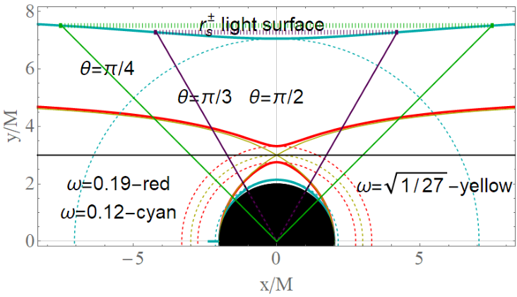
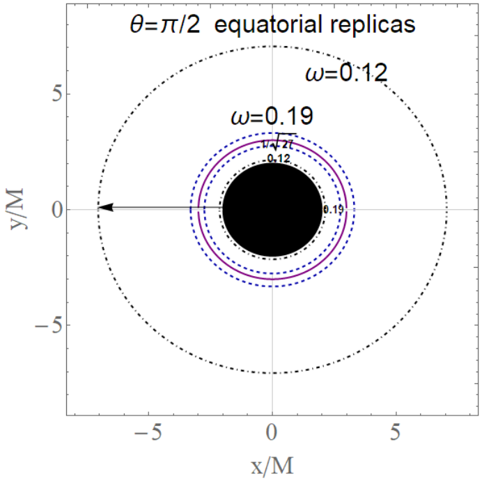

The observational relevance of these structures lies in the fact that it is possible to find replicas introduced here of effects and quantities dependent on relativistic frequency , and since these strictly constrain the jet emission, the presence of frequency replicas should appear in a region close to the horizon and in one far from the BH –Figs 5,6.
3.5 Impacting conditions
There are two major cases to consider in the investigation of the constraints of the toroidal configurations collision. (a) The case we mainly consider here is the occurrence of jet collision with accreting configurations. In this case we consider a one dimensional problem for the accreting disks, fixing the angular momentum parameter for the accretion, and we consider quantities evaluated in . For proto-jets we fix the parameter , considering quantities evaluated at . Eventually, we can consider a quiescent torus where the specific angular momentum can be in or (b) It should be noted that a further possibility is the collision occurring with an internal closed configuration (internal Roche lobe “embracing” the BH horizon) which is considered here in , or and therefore it comprises different cases.
A further situation to be analyzed comprised the role of the configurations embracing the BHs at and . The cases (a) and (b) represent very different scenarios. The case of quiescent configurations is indeed much more complex than the case of impact between cusped tori and jet-emission, and dependent on the boundary conditions. It is clear that for the impact conditions we have to evaluate the elongation on the plane of symmetry of the torus, the maximum vertical height, that ultimately defines the thickness of the disks increasing with and . However, for , the quiescent configuration is at large distance from the central attractor, and effects of the torus self–gravity starts to be relevant. The orbital region of location for tori with extends to infinity. However and are, for , increasing functions of the radius, implying the presence of closed configurations which can be also very large. The maximum limit for -parameter of the closed, cusped or quiescent, tori is . For these special tori we are mainly interested on the location of the inner edge. Below we enlist the expression of the equipotential surfaces defining the configurations, and we introduce a relation reducing the independent parameters for cusped (tori and proto-jets) surfaces.
The equipotential surfaces
We can address the problem directly solving the equipressure-equipotential surfaces constant for a generic . Clearly, the constant pressure levels provide the inner edge and, for closed surfaces, the outer edges of the configurations. We therefore introduce the quantity
| (32) |
showed in Figs 6. We obtain in Cartesian coordinates
| (33) |
or, alternatively the surfaces
The equipotential surfaces satisfy both the cancellation of the radial and polar gradient (defining the “verticality” of the configuration) and therefore the two projections of the Euler equations, fixing also the verticality of the disk, as we shall see in detail in Sec. (4).


Reducing proto-jets parameters :
We can relate to by eliminating the critical pressure radial dependence , obtaining the following function :
| (34) |
represented in Figs (6,15), or alternately the relations defined as
| (35) |
where
| (36) |
is either , for proto-jets, or for accreting configurations, which is represented in Figs 12 or evaluated in the centers of maximum pressure. These relations connect a pair of radii from the condition constant, identifying a torus and eventually the associated HD (topological) instability with the correspondent value of ; accordingly there are two parameters such that for and for and for , where clearly and are respectively and or for the fixed .
4 Tori characteristics, limiting conditions and pressure gradients
In this section we discuss the maximum and minimum density and pressure and the thickness of the disk related to the radial gradient of the pressure. We will explore the disk verticality by the analysis of the radial gradient of the pressure. The analysis developed in the frame of RAD models is characterized by the intensive use of a multi-parametric analysis on important characteristics of the tori. In this section we investigate the configuration center, i.e. the maximum pressure point, focusing in particular on the projection of the morphological maxima on the equatorial plane. We discuss the inner edge, the center and the morphological maximum in dependence on different tori parameters. The morphological maximum will be found from the RAD rotational law, showing the disk vertical structure determined by the radial structure through the agglomeration rotation. The center of the maximum pressure point of the configurations is given by
| (37) | |||
| (38) |
(for compare with Eq. (–The inner edge, the center and the maximum)). The center of the orbiting torus is the point, on its equatorial plane, of the maximum pressure and density. The location of this point depends on one torus parameter, or , determined as minimum point of the effective potential function regulating the force balance in the torus. In Eq. (37) the center depends on the specific angular momentum of the fluid, and it is obtained by inverting the function in the range .


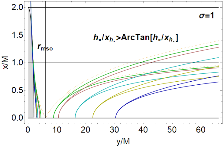


The projections of the morphological maxima on the equatorial plane are
| (39) |
where
see Fig.(13). is the point of maximum, on the equatorial plane, of the external and internal Roche lobe respectively. This is obtained by using function of Eq. (9) on a fixed equatorial plane (the center lies on the axis), therefore the morphological maximum points on the toroidal surfaces can be obtained calculating
| (40) |
where here there is accordingly respectively. For the tori on planes others then the equatorial, solutions are rotated according to Eq. (9)–see Figs (9,10,12,13,14,15).
The morphological maximum point for the outer Roche lobe, point , the projection of the maximum morphological on the equatorial plane, the maximum pressure point , and the morphological maximum are shown in Fig.(13). (In this work we focus attention on the outer lobus, especially in the case of quiescent tori. The meaning of the inner configuration at equal and embracing the BH needs to be explored in more detail, see for examplePugliese&Montani 2015).
- –The inner edge, the center and the maximum
-
It is well known that the point of maximum density and maximum (HD) pressure in the torus (the minimum of the effective potential of the fluid as function of ) does not correspond to the morphological maximum point of the torus surface, while this can happen for the morphological minimum of the surface and the minimum of the pressure/density (which is , maximum point of the effective potential as function of if it exists). However the two points, the minimum and maximum point of the toroidal surface and and , i.e., the maximum pressure point and center of disk and inner edge of disk (which corresponds to the minimum of pressure) are related. The two points of pressure and morphological maximum coincide when projected on the equatorial plane of the torus in the sense explained below, and therefore the maximum is directly given by the angular distribution calculated on the equatorial planes, as evident from the Figure (6) and (7). This analysis fixes also the role of the radial gradient of the pressure in the tori in determining the torus verticality. Explicitly, the following transformations apply
(41) or also —see Figs 9,10,13– where
(42) where
for see Eq. (37)–Figs 11. is the component found from substituting where . We note that the quantity is related to the frequency. In fact the center is a point of curve at , for any . The maximum of the surface depend on and it can exist for , for and . These are related for the critical cusped configuration in the implicit relation . To clarify this point we report below the exact form
(43) where
(44) where , and are solutions of , the morphological maximum is actually connected to the maximum of pressure and density. Notably this relation is independent from but it holds, for each , for any , therefore it holds also for non-critical configurations. Interestingly, this seems to prove that the distribution of specific angular momentum for the fluid has a predominant role in the determination of the disk structure with respect to the effective potential function (values ). Therefore we bounded the maxima and minima of pressure / density to the maxima and minima of the toroidal surface. Then, we note that corresponds to (on each equatorial plane) and therefore can be obtained as solution of . It is clear that the solves the problem for . In this context is related to .
Maximum from the RAD rotational law We can prove that the analysis of the morphological maximum leads to the an angular momentum distribution with explicit dependence on :
(45) 


Figure 16: Black region is the BH. Left upper panel: of Eq. (46) as function of for different values of the specific angular momentum . Center upper panel: limiting radius Eq. (48) for different values of the specific angular momentum , colors are as right panel. Radii (marginally stable orbit, marginally bounded orbit and photon circular orbit) are shown. Right upper panel: a zoom. Solutions for are shown. Other solutions are (with ). Bottom left panel: defined in Eq. (46) providing the center, and the cusp edge, see also Figs 8. Dotted curves are configurations at various . represent the limiting condition for these configurations. Bottom right panel: a zoom including the surfaces =constant (dashed-orange curves) related to von Zeipel curves. Explicitly, and , locating the cusp can be given as unique solution as follows:
(46)
- –Centers and inner edges as functions of
-
It is convenient to express the center and inner edge of critical configurations (the cusps) explicitly in terms of the parameter
(47) where
solutions of equation which provides as functions of –see Fig. 17. (The function evaluated on provides which is independent from and therefore we cannot use the RAD energy function to directly provide limits on the morphological maximum of the surface.). Note we can use function in Eq. (34,41,–The inner edge, the center and the maximum,46).

Figure 17: Points of maximum pressure and density in the disk (disk center) and minnimum points of pressure and density , () of Eq. (47). Radius is the cusp of closed tori, is the cusp of open configurations (proto-jets).
Below we list some limiting surfaces constraining the proto-jets emission considered above: the von Zeipel surfaces, the radius , the light-surfaces, the surfaces derived from the normalization conditions and the surfaces at .
The limiting conditions
For the limiting conditions, from Figs 16 it is clear that we have to consider the three regions bounded by and where the surfaces are open, or from to (which is the stationary surface). The results of this analysis are shown in Figs 9,10,16,13, 11,12. These surfaces also include the von Zeipel surfaces role as limiting conditions for jets– Eq. (7).
- •
- •
–Light-surfaces of Eq. (23)
(we can consider also the substitution , expressing the light surfaces in terms of the specific fluid angular momentum).
- •
–Normalization conditions From the normalization condition on the fluid four velocity (constraining the stream by the causal structure) we obtain the quantity L2S. Considering Eq. (25) there is , where . Therefore the limiting value is , but frequency provides limiting conditions , solving also for a generic . Surfaces and are related, as it is .
Among these surfaces we also use condition implying the orbits and momenta
| (49) |
is shown in Figs 10–Fig. 18-clearly there is a critical point in , for .


Some of these limiting surfaces are related to the HD structures, solutions of the Euler equations for the problem, others are more strictly related to the geometrical constraints provided by the causal structure.
As clear from Figs 7,9,10, we can identify a region around the rotational axis of the toroidal configurations where there are no solutions of the Euler equation, to represent matter funnel constraints, being therefore darker regions–Figs (7). The extension of this region, developed along two boundaries estimated as . The configurations very close (embracing) the horizon are in the range ( is defined in Eq. (26)). Region to be considered has extension by , implying the condition (where is the torus height at its morphological maximum point), where both and , defining a further limit, depend on the fluid angular momentum. Boundaries of darker regions are, asymptotically, collimated to with increasing , while the center of maximum pressure for these configurations moves outwardly. In this context we can further reduce the darker region, for example in Figs 7,9,10, to a region bounded by the surfaces . To evaluate collimation conditions, we fix an open or closed solution and proceed to study the intersection with a second configuration under particular conditions.
On the polar gradient
The polar and radial gradients of the effective potential are related to the pressure gradients due to the Euler equations. The gradients are studied in Figs 19. The effective potential gradients ratio coincides with the ratio of the pressure gradients and related density gradient ratios in the disk. We can study the integrals of related differential equations investigating more closely the equi-pressures surfaces. This investigation shows the role of polar and radial gradients in systems with toroidal symmetries. Furthermore, integration of the partial differential equations shows the role of the gradients in the determination of the geometric thickness of the torus. The analysis proves also that the rotational law of the RAD can be derived from the radial gradient and the radial gradient determines also the points of maximum pressure density in the disk (the center) connected to the (morphological) maximum point of their external Roche lobe.


The solution of the partial differential equation of the first order for the pressure, in the ratio of the gradients, provides the function
| (50) |
solutions for the ratio of the pressure gradients. We take constant, as in Figs 19. We have already seen how the disk verticality is determined by its radial gradient, derived by its rotational law . By using the parametrization introduced in Sec. (3.4) on the metric Killing bundles we solve the problem for
| (51) |
However to fix the class of solutions, for parameter to get the toroidal surfaces, the constant has to be properly chosen. For this purpose we consider the radial gradient of the function and solving the problem of its zeros we find a function which provides the correct rotational law
| (52) | |||
we note that this can be also written immediately using Eqs (13) in terms of epicyclic frequencies, interpreted therefore in terms of oscillation frequencies. It is worth noting however, as also clear from Figs 19, that is a maximum of the function which is actually negative at , null at , and the horizon is an asymptote.
5 Collisions and intersections
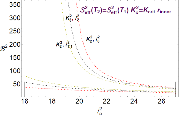
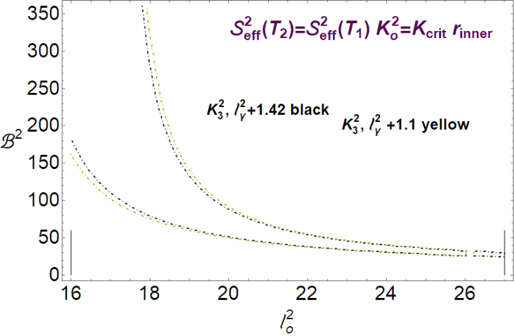
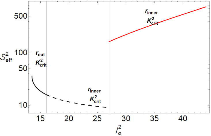
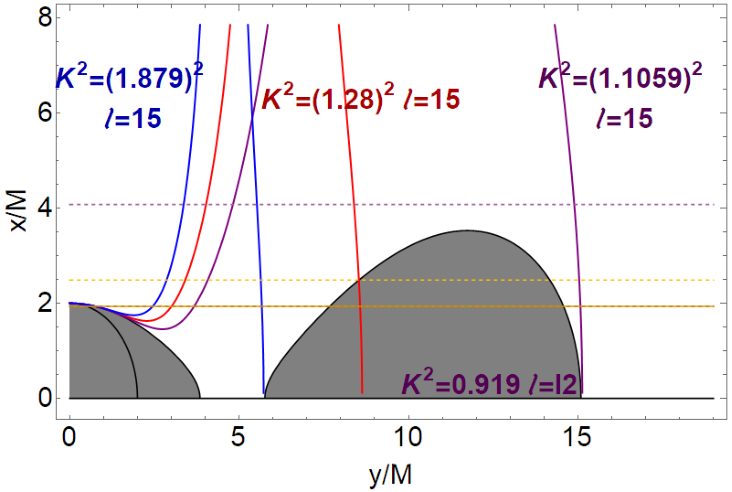
In this section we explore the intersections between the toridal surfaces in different topologies and with fluid specific angular momentum in the range or , and the open surfaces. In particular we consider the open surfaces with cusps and the limiting surfaces and (light surfaces). In general, we assume the open surfaces are on a generic plane , while we fix the torus on the equatorial plane . More generally, the analysis of the collision conditions with the surrounding matter addresses the problem of jet launching point location and jet structure (collimation and velocities). Considering the toroidal surfaces defined by the functions , the first immediate way to obtain the collision conditions, according to the values of different parameters, is to explore the surfaces crossing. This analysis is mostly reduced to an algebraic multi-parametric condition. We take explicitly the four topological solutions: closed, quiescent, closed cusped surfaces and the proto-jets, we consider also the limiting surfaces (for example the three radii , and ). All these surfaces depend on one or both parameters and , according to the morphological conditions assumed for the toroidal surfaces. In some circumstances, for example in the case of cusped surfaces, we can make use of Eqs (35,36,34) to fix as function of or viceversa as functions of . For a non-cusped surface there is (or ). It is clear that in the determination of a (unique) couple for the surfaces collision we obtain a relation where are a couple of reduced parameters, , for the two surfaces respectively, index is used for quantities related to the configuration . In general we consider a couple constituted by a closed torus conveniently considered on its equatorial plane or , reducing then . One condition can be , , leaving undetermined the angular relation, we set and . Therefore we consider
| (53) |
where , , and , . Using the disks symmetries, we concentrate mainly on the plane and , although clearly a jet on and is in this case not considered. Very special cases are , or i.e. orthogonal configurations. A limiting case for the equations is therefore the case (note that there is always a phase difference in these relations due the configurations relative orientations). We consider also the case .
The relation to be considered to evaluate the crossing conditions is , where and are two configurations under analysis, one configuration will be denoted with parameters , and plane . We assume a torus (closed configuration) fixed, without loss of generality, on its equatorial plane and the second configuration defined by different parameters on different planes. Clearly the points and in the frame adapted to the torus are assumed to be the crossing point with the second configuration. The solution on the equatorial plane is as follows ():
| (54) |
alternatively, in terms of parameter
| (55) |
One can express the collision conditions directly in terms of the contact point
| (56) | |||
In general the crossing of a configuration with a surface on any plane with the open limiting configurations is rendered by the following conditions , where . We obtain for this problem the solution
| (57) |
alternatively
| (58) |
We then proceed to consider the crossing between a closed torus and an open surface. Some points are of particular interest, for example, when the collision point is close to the edges of the configuration in accretion, or the cusp of a proto-jet, showing a geometrical correlation between the two processes (Pugliese&Stuchlík 2017). For this purpose we consider , or (the outer edge of a cusped torus), here and in the following we consider and . In general the conditions to be considered are ( belongs to the Boyer surface associated to and tori) and for cusped or quiescent tori. However, in the case of cusped tori, the condition can be or, for the equipotential level superior of the maximum critical value (), we can adopt the condition where is a fixed point. Therefore, we first fix for accretion condition, where , while the second case we consider is a proto-jet emission. We can find the exact analytical form of these solutions, represented also in Figs 20.
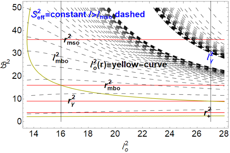
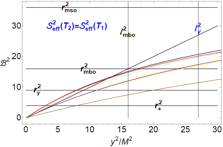
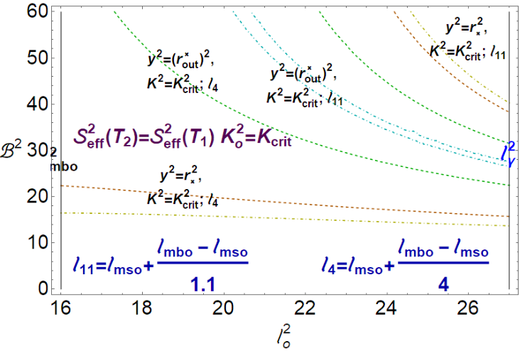
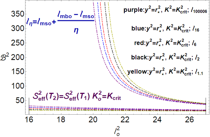
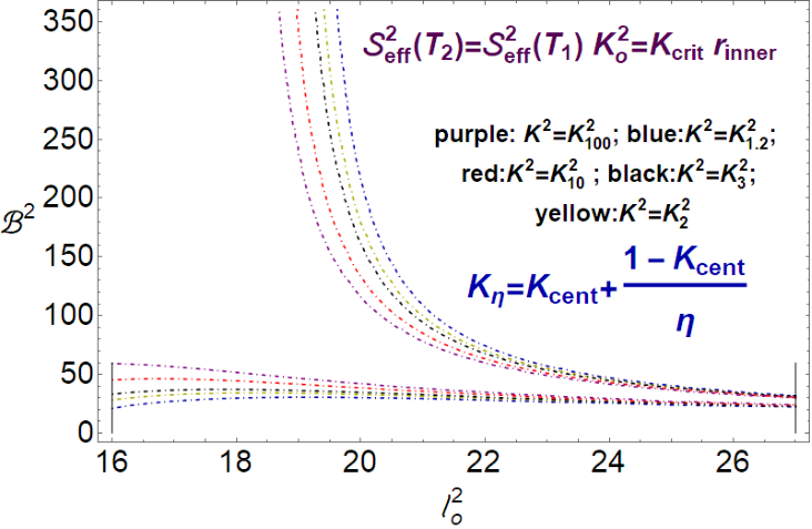
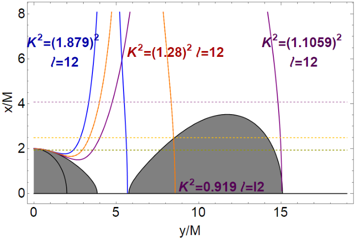
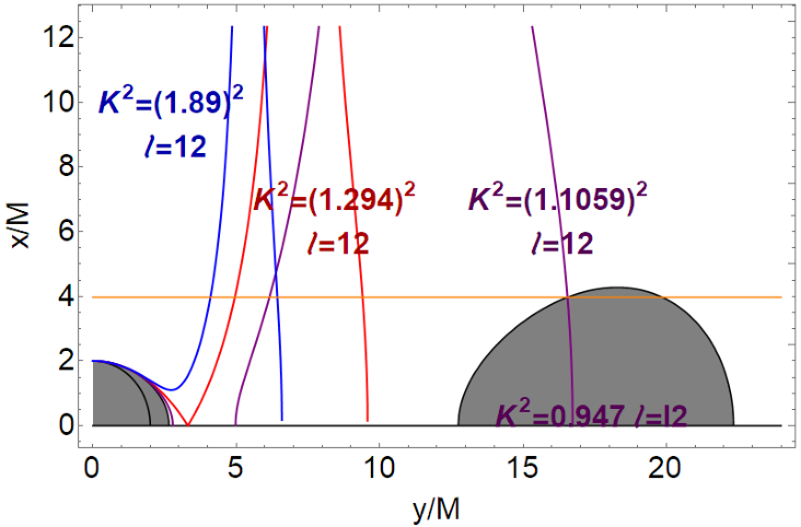
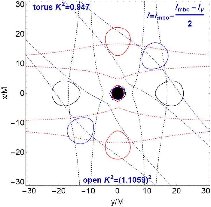
Crossing solutions are
| (59) | |||
| (60) | |||
we solved for the solutions and and for Eq. (60) (on the equatorial plane there is ). More specifically, solving the problem on the unique symmetry plane we find:
| (61) | |||
| (62) | |||
The condition of crossing at equal parameters implies , leading to the set of solutions:
where (conditions at equal can be easily reduced as well)–(see Figs 20,21,22).
6 Proto-jet collimation and toroidal magnetic field
We address the role of a toroidal magnetic field in the possible open surface collimation along an axis crossing the attractor center. Here we consider again the equatorial plane case, , investigating if the proto-jet cusp and the open matter funnel are shifted inwardly tending to collimate with respect to the non-magnetized case. In Pugliese&Montani 2013 it has been shown that the torus geometrical thickness remains basically unaffected by the toroidal magnetic field, tending however to increase or decrease slightly depending of a combination of many factors such as the magnetic, gravitational and centrifugal effects. We used the toroidal “Komissarov” magnetic field model developed in Komissarov 2006; Montero et al. 2007.
Assuming a barotropic equation of state, we consider the force-free approximation with an infinitely conductive plasma, , where is the Faraday tensor and is the fluid four-velocity. Using the equation , where is the magnetic field, we find the relation , is the relativistic velocity of the fluid. Moreover, we assume and . Within the conditions from the Maxwell equations there is, that is satisfied for or (=constant). This implies that the assumptions and lead to . (The presence of a magnetic field with a predominant toroidal component can be reduced to the disk differential rotation, which plays the part of the generating mechanism for the the magnetic field (Komissarov 2006; Montero et al. 2007; Horak&Bursa 2009; Hamersky&Karas 2013; Parker 1955; Parker 1970; Yoshizawa et al. 2003; Reyes-Ruiz&Stepinski 1999).) The magnetic field is therefore (Adamek&Stuchlik 2013; Stuchlík, et al. 2020)
| (63) |
where is the magnetic pressure, is the fluid enthalpy, and and are constant. The introduction of the Komissarov magnetic field maintains the integrability conditions on the Euler equation which can be exactly integrated, resulting
| (64) | |||
where and are functions to be fixed by the integration. For , there is We consider then where
| (65) |
Therefore there is and we consider the equation for the constant. The effective potential function, modified by the introduction of the magnetic field reads
| (66) |
where , assuming the enthalpy to be a constant, where the ratio gives the comparison between the magnetic contribution to the fluid dynamics through , and the hydrodynamic contribution through the specific enthalpy . Potential for reduces to the effective potential for the non-magnetized case . For the magnetic field does not affect the Boyer potential and therefore the Boyer surfaces. (In the limit case , the magnetic field , does not depend on the fluid enthalpy.).
Note that the magnetic pressure is regarded here as a perturbation of the hydrodynamic component, it is assumed that the Boyer theory of rigid rotating surfaced in GR remains valid and applicable in this approximation. Conveniently one can introduce as done in Pugliese&Montani 2018; Pugliese&Stuchlik 2020b; Pugliese&Montani 2013 the parameter .
The modified specific angular momentum distribution of the eRAD and the modified function , with the contribution of the magnetic field are
| (67) |
where and in the limiting cases (1) and ; (2) ; or (3) provide the rotational law in absence of magnetic field. For a deeper discussion on the interpretation and role of the limiting values on the magnetic parameters we refer to Pugliese&Montani 2018; Pugliese&Stuchlik 2020b; Pugliese&Montani 201333 3 The range of parameter is divided into two regions, say and , with a subrange extreme . The case is indeed interesting because the magnetic field loops wrap around with toroidal topology along the torus surface (Pugliese&Montani 2013). For closed surfaces (tori) are approximately those studied in the case , for there are closed surfaces in the limit , which is in agreement with the situation when the contribution of the magnetic pressure to the torus dynamics is regarded as a perturbation with respect to the HD solution.. We note however that for we obtain . In Figs 23 we show the modified and some toroidal surfaces.


As shown in Figs 23, although qualitatively an effect appears in the sense of funnels squeezing along the rotational axis, from this first analysis there is no quantitative relevant collimation effect as shown in Pugliese&Montani 2013 for a squeezing effect (exploring the disk thickness changing the physical characteristics of the torus particularly its magnetic field) on the equatorial plane for the toroidal configurations closed and orbiting a Schwarzschild central BH.
7 Conclusions
We explored the possibility of jets collisions with misaligned accreting tori orbiting around a SMBH. We use a model of misaligned tori orbiting one central static SMBH which may be host for example in AGNs, since several observational evidences associate such structures to different periods of accretion of SMBHs. We studied the geometric limits given by the black hole geometry on the possibility of jets, created by tori in vicinity of the central SMBH, to collide with obscuring inclined toroidal structures, which are extended on large distance from the SMBH. There are several indications showing a jet emission-accretion disk correlation. The aggregates of misaligned multi tori orbiting one central SMBH with different matter flows include proto-jets. As consequences of the agglomeration internal ringed structure, orbiting toroidal jets shell and jets may interact with the surrounding matter, leading to tori-proto-jets collision. The location of jet “launching point” in proto-jets, which are interpreted as limiting configurations for orbiting funnels of matter in toroidal symmetry, is associated to the emergence of a cusp, that is a minimum of pressure and density in the extended orbiting matter. The fluid fills any (closed) equipotential surfaces with a purely toroidal flow.
The interaction with surrounding matter provides possible jets replenishment mechanism. This mechanism may follow the impact of accreting material on an inner configuration that can be associated eventually to the emergence of chaotic processes. For the analysis of these agglomerations, we used GRHD tori in the RAD frame introduced in Sec. (2). Proto-jet emission hypothesis and possible shells of jets in the RAD frame have been discussed in Sec. (2.1). Proto-jet emission has been constrained by GRHD thick tori characteristic frequencies, as shown in the analysis of Sec. (2.2). Then constraints on the GRHD systems are addressed in Sec. (3). There are “darker regions” along the fluid rotation axis, bounded by special surfaces of GRHD origins. A torus, quiescent or cusped, can impact a jet at any angle. Thus the possibility of a torus, quiescent or cusped, filling the proto-jet darker region has to be included. Cusped tori are very much constrained in terms of locations, dimension and velocity component. For quiescent tori there is a great degree of indetermination on the location, velocity components and density. Such toroids can range from the small quiescent tori, which are slower rotating, that is with , and located close to accreting region, to the very large tori, which are faster rotating, , and located far away from the central BH. Some relevant limiting radii have been identified, with a HD origin and a GR nature related to the causal structure imposed by the geometric background determined by the central SMBH, for example the “asymptotic radius” derived from the normalization conditions–see Sec. (3.1). Limiting conditions on frequency and momentum are analyzed in Sec. (3.2). In Sec. (3.3) we introduced the stationary observers and light-surfaces determining replicas discussed in Sec. (3.4), significant for the possible observational evidence of the jet shells. Impacting conditions are discussed in Sec. (3.5). Tori characteristics, limiting conditions and pressure gradients in the tori are the focus of Sec. (4). We proved then that the radial gradient of pressure in fact determines the disk verticality and the center of maximum pressure in the disk is related to the morphological maximum of the tori surfaces. In Section (5) we explored the toroidal surfaces collisions in different topologies. Finally, the role of a toroidal magnetic field in the possible proto-jet collimation is analyzed in section (6). Although from a first analysis, the toroidal magnetic field does not appear to show a significant quantitative effect on the collimation or shift of the cusp associated with the proto-jets, it cannot be excluded that in conjunction with dragging of frame, in the case of a rotating attractor, a toroidal magnetic field may instead be significant. (For more discussion on general relativistic exact models of magnetic field around rotating compact sources and dragging effects see Mirza 2017; Petri 2016; Gutierrez&Pachon 2015; Herrera et al. 2006).
Collision emergence and the stability properties of the aggregates have been considered at different inclination angles relative to a fixed distant observer. Therefore constraints to jet-torus impact are provided in terms of misalignment angles and tori parameters, exploring also the observational evidences of SMBH host configurations. (It is possible to reduce the results given here, expressed in terms of conditions on the and parameters, in terms of the flow velocity components, and , the relativistic velocity and the frequencies.). In this respect we investigated the constraints provided by the light surfaces, defining structures related to recently introduced Killing metric bundles (Pugliese& Quevedo 2021; Pugliese&Montani 2020; Pugliese&Quevedo 2019a; Pugliese&Quevedo 2019b; Pugliese& Quevedo 2019c). These structures pointed out the existence of orbit-replicas that could host shadowing effects as replicas (horizon replicas in jet shells) of the emissions in regions close and far from the BH. These orbits are characterized by equal limiting photon orbital frequency. The observational relevance of the bundles could be explained by looking at their exact definition. For a given function of the limiting light-like toroidal orbital frequencies, there are two orbits and two planes such that there is and, as per definition of replica, there is . The regions defined by and can be interpreted as presenting replicas of the proprieties, where if is a circle very close to the attractor then the second point is located far from the attractor (note that this relation is independent from the azimuthal angle and it is eventually even reducible to a simplest relation between the couple of radii ).
The investigation clarifies also the role of the pressure gradients of the orbiting matter and the essential role of the radial gradient of the pressure in the determination of the disk verticality. We investigated the possibility that a toroidal magnetic field could be related to the collimation of proto-jets: including a strong toroidal magnetic field, developed in Komissarov 2006; Montero et al. 2007, we addressed the specific question of jets collimation. The assumptions of these simplified models of thick (stationary) GRHD disks and a central Schwarzschild BH can be a good approximation of more refined dynamical models, providing an estimation of different aspects of tori construction as elongation on their symmetry plane and the critical pressure points. This analysis is therefore the first step to the exploration of the wider scenario in which the RAD orbits a central Kerr attractor is involved, relating directly jet emission with energy extraction from the central BH at the expense in general of rotational energy, considering also Blandford– Znajek process, the magnetic field lines torque, magnetic Penrose process(Stuchlík, et al. 2020) and the Lense–Thirring precession effects.
References
- Abramowicz&Fragile (2013) Abramowicz M. A. & Fragile P. C. 2013, Living Rev. Relativity, 16, 1
- Abramowicz et al. (1978) Abramowicz M.A., Jaroszyński M. J& Sikora M. 1978, A&A, 63, 221
- Adamek&Stuchlik (2013) Adamek K. & Stuchlik Z. 2013, Class. Quantum Grav. 30, 205007
- Alig et al. (2013) Alig C., Schartmann M., Burkert A., Dolag K. 2013, ApJ, 771, 2, 119
- Aly et al. (2015) Aly H., Dehnen W., Nixon C., & King A. 2015, MNRAS, 449, 1, 65
- Balbus&Hawley (1998) Balbus S. A.& Hawley J. F. 1998, Rev. Mod. Phys,. 70, 1
- Blaes (1987) Blaes O. M. 1987, MNRAS227, 975
- Blanchard et al. (2017) Blanchard P. K. 2017, et al., arXiv:1703.07816 [astro-ph.HE]
- Blaschke&Stuchlík (2016) Blaschke M. & Stuchlik Z. 2016, Phys. Rev. D, 94, 8, 086006
- Bonnell&Rice (2008) Bonnell I. A., & Rice W. K. M. 2008, Science, 321, 1060
- Bonnerot et al. (2016) Bonnerot C., Rossi E. M., Lodato G. 2016, MNRAS, 455, 2, 2253
- Boyer (1965) Boyer R. H. 1965, MPCPS, 61, 527
- Carmona-Loaiza et al. (2015) Carmona-Loaiza J.M., Colpi M., Dotti M. et al 2015, MNRAS, 453, 1608
- Chatterjee et al. (2020) Chatterjee K. , Younsi Z. , Liska M., Tchekhovskoy A., et al. 2020,[arXiv:2002.08386 [astro-ph.GA]].
- Contopoulos et al. (2012) Contopoulos I. , Kazanas D., Papadopoulos D. B. 2013, ApJ, 765, 2, 113
- Dexter&Fragile (2011) Dexter J. & Fragile P. C. 2011, ApJ, 730, 36
- Dogan et. al (2015) Dogan S., Nixon C., King A., et al 2015, MNRAS, 449, 2, 1251
- Dyda et al. (2015) Dyda S, Lovelace R.V.E., et al. 2015MNRAS, 446, 613
- Fragile&Blaes (2008) Fragile P. and Blaes O. M. 2008, ApJ, 687, 757
- Franchini et al. (2019) Franchini A., Martin R. G. , Lubow S.H. 2019, MNRAS, 485, 1, 315–325
- Gafton et al. (2015) Gafton E., Tejeda E. , et al 2015MNRAS, 449, 1, 771
- Greenhill et al. (2003) Greenhill L. J. , Kondratko P. T. , Lovell J. E. J., Kuiper T. B. H., et al.,2003, ApJ, 582, L1
- Gutierrez&Pachon (2015) Gutierrez–Ruiz A.F., Pachon L. A. 2015, Phys. Rev. D, 91, 124047
- Hamersky&Karas (2013) Hamersky J. &V. Karas 2013, A&A, 555, A32
- Herrera et al. (2006) Herrera L, Gonzalez G.A., Pachon L.A., Rueda J.A. 2006, Class. Quantum Grav. 23, 2395
- Herrnstein et al (1996) Herrnstein J. R., Greenhill L. J. , Moran J. M. 1996, ApJ, 468, L17
- Horak&Bursa (2009) Horak J.& Bursa M., “Polarization from the oscillating magnetized accretion torus,” in R. Bellazzini, E. Costa, G. Matt&G. Tagliaferri X-ray Polarimetry, Cambridge University Press (2010) arXiv:0906.242
- King&Nixon (2018) King A. and Nixon C. 2018, ApJ, 857, 1, L7
- Komissarov (2006) Komissarov S. S. 2006 , MNRAS, 368, 993
- Kovar et al. (2010) Kovar J., O. Kopacek, Karas V. and Stuchlik Z. 2010, Class. Quant. Grav. 27, 135006
- Kovar et al. (2014) Kovar J., Slany P., Cremaschini C., et al. 2014 Phys. Rev. D, 90, 4, 044029
- Kovar et al. (2016) Kovar J., Slany P., Cremaschini C., et al. 2016 Phys. Rev. D, 93, 12, 124055
- Kovar et al. (2011) Kovar J., Slany P., Stuchlik Z., Karas V., C. Cremaschini and J. C. Miller 2011, Phys. Rev. D, 84, 084002
- Kozlowski et al. (1978) Kozlowski M., M. Jaroszynsk& Abramowicz M. A. 1978, A&A63, 1–2, 209–220
- Lasota et al. (2016) Lasota J. P., Vieira R. S. S. , Sadowski A., Narayan R., & Abramowicz M. A. 2016, A&A, 587, A13
- Lei et al. (2008) Lei Q. , Abramowicz M. A. , Fragile P. C. , et al. 2008 A&A, 498, 471
- Liska et al. (2019) Liska M., Tchekhovskoy A. , Ingram A., van der Klis M. 2019, MNRAS, 487, 1, 550–56
- Lodato&Pringle (2006) Lodato G. & Pringle J. E. 2006, MNRAS, 368, 1196
- Lyutikov (2009) Lyutikov M. 2009, MNRAS, 396, 3, 1545–1552
- Madau (1988) Madau P. 1988, ApJ, 1, 327, 116-127
- Mahlmann et al. (2018) Mahlmann J. F., Cerda-Duran P. and Aloy M. A. 2018, MNRAS, 477, 3, 3927
- Miller et al. (2015) Miller J. M., Kaastra, J. S., Coleman Miller M. C., et al 2015Nature, 526, 542–545
- Miller-Jones et al. (2019) Miller-Jones J. C., Tetarenko A. J., Sivakoff G. R., Middleton M. J., et al. 2019 Nature, 569, 374-377
- Mirza (2017) Mirza, B.M. 201, apj, 847, 73
- Montero et al. (2007) Montero P. J. , Zanotti O. , Font J. A.,& Rezzolla L. 2007, MNRAS, 378, 1101
- Nixon et al. (2013) Nixon C, King A, & Price D. 2013, MNRAS, 434, 1946
- Parker (1955) Parker E. N. 1955, ApJ, 122, 293
- Parker (1970) Parker E. N. 1970, ApJ, 160, 383
- Petri (2016) Petri, J. 2016, A&A, 594, A112
- Pugliese&Montani (2013) Pugliese D. &Montani G. 2013, EPL, 101, 1, 19001
- Pugliese&Montani (2015) Pugliese D.&Montani G. 2015, Phys. Rev. D, 91, 083011
- Pugliese&Montani (2018) Pugliese D.&Montani G. 2018, MNRAS, 476, 4, 4346
- Pugliese&Montani (2020) Pugliese D.and Montani G. 2020, Entropy, 22, 402
- Pugliese&Quevedo (2018) Pugliese D. and Quevedo H. 2018, Eur. Phys. J. C, 78, 1, 69
- Pugliese&Quevedo (2019a) Pugliese D.and Quevedo H. 2019a, [arXiv:1910.04996 [gr-qc]]
- Pugliese&Quevedo (2019b) Pugliese D and Quevedo H 2019b, [arXiv:1910.02808 [gr-qc]]
- Pugliese& Quevedo (2019c) Pugliese D. and Quevedo H. 2019c, Eur. Phys. J. C, 79, 3, 209
- Pugliese& Quevedo (2021) Pugliese D.and Quevedo H 2021., European Physical Journal C, 81, 258
- Pugliese&Stuchlík (2015) Pugliese D.&Stuchlík Z. 2015, ApJS, 221, 2, 25
- Pugliese&Stuchlík (2016) Pugliese D. &Stuchlík Z. 2016, ApJS, 223, 2, 27
- Pugliese&Stuchlík (2017) Pugliese D.& Stuchlík Z. 2017, ApJS, 229, 2, 40
- Pugliese&Stuchlik (2018a) Pugliese D.& Stuchlik Z. 2018a, Class. Quant. Grav., 35, 18, 185008
- Pugliese&Stuchlík (2018a) Pugliese D.&Stuchlík Z. 2018a, Class. Quant. Grav. 35, 10, 105005
- Pugliese&Stuchlík (2018b) Pugliese D.& Stuchlík Z. 2018b, JHEAp, 17, 1
- Pugliese&Stuchlík (2019) Pugliese D. & Stuchlík Z. 2019, Eur. Phys. J. C, 79, 4, 288
- Pugliese&Stuchlik (2020a) Pugliese D.& Stuchlik Z. 2020a, MNRAS, 493, 4229
- Pugliese&Stuchlik (2020b) Pugliese D.& Stuchlik Z. 2020b, Class. Quantum Grav. 37, 195025
- Reyes-Ruiz&Stepinski (1999) Reyes-Ruiz M., Stepinski T. F. 1999, A&A, 342, 892–900
- Sadowski et al. (2016) Sadowski A., Lasota J. P., Abramowicz M. A. & Narayan R. 2016, MNRAS, 456, 4, 3915
- Shakura (1973) Shakura N.I. 1973, Sov. Astronomy, 16, 756
- Shakura&Sunyaev (1973) Shakura N.I. & Sunyaev R. A. 1973,A&A, 24, 337
- Sikora (1981) Sikora M. 1981, MNRAS, 196, 257
- Slany et al. (2013) Slany P., Kovar J., Stuchlik Z. and Karas V. 2013, ApJS, 205, 3
- Stuchlik (1980) Stuchlik Z. 1980, BAICz, 31, 129
- Stuchlik (1983) Stuchlik Z. 1983, BAICz, 34, 129
- Stuchlík (2005) Stuchlik Z. 2005, Modern Physics Letters A, 20, 561
- Stuchlik et al. (2017) Stuchlik Z., Blaschke M.,& Schee J. 2017, Phys. Rev. D, 96, 104050
- Stuchlík & Hledík (1999) Stuchlik Z., & Hledík S. 1999, Phys. Rev. D, 60, 044006
- Stuchlík et al. (2016) Stuchlik Z., Hledík S., & Novotný J. 2016, Phys. Rev. D, 94, 103513
- Stuchlík et al. (2011) Stuchlik Z., Hledík S., Truparová K. 2011, CQGra, 28, 15501
- Stuchlík, et al. (2020) Stuchlik Z., Kološ M. , Kovar J., et al 2020, Univ, 6, 26
- Stuchlík et al. (2013) Stuchlik Z., Kotrlová A. , Török G. 2013, A&A, 552, A10
- Stuchlík & Kovář (2008) Stuchlik Z., &Kovar J. 2008, Int. Journ. of Modern Physics D, 17, 2089
- Stuchlík et al. (2000) Stuchlik Z., Slany P. & Hledík S. 2000, A&A, 363, 425
- Stuchlík et al. (2009) Stuchlik Z., Slany P., Kovar J. 2009, CQGra, 26, 215013
- Stuchlik et al. (2005) Stuchlik Z., Slany P., Torok G. and Abramowicz M. A. 2005, Phys. Rev. D, 71, 024037
- Tchekhovskoy et al. (2010) Tchekhovskoy A., Narayan R., and McKinney J. C. 2010, ApJ, 711, 50–63
- Teixeira et al. (2014) Teixeira D. M., Fragile P. C., Zhuravlev V. V. et al 2014, ApJ, 796, 2, 103
- Trova et al. (2016) Trova A., Karas V., Slany P. et Kovar J. 2016, ApJS, 226, 1, 12
- Trova et al. (2018b) Trova A., Schroven K., Hackmann E., et al,. 2018 Phys. Rev. D, 97, 10, 104019
- Trova et al. (2018c) Schroven K., Trova A., Hackmann E. et al 2018, Phys. Rev. D, 98, 2, 023017
- Uzdensky (2004) Uzdensky D. A. 2004, ApJ, 603, 652–662
- Uzdensky (2005) Uzdensky D. A. 2005, ApJ, 620, 889
- Yoshizawa et al. (2003) Yoshizawa A., S.Itoh I., Itoh K. , 2003 Plasma&Fluid Turbulence: Theory and Modelling, CRC Press
- Zubovas&King (2008) Zubovas K. , King A., 2008arXiv:1901.02224 [astro-ph.GA]