1
RLibm-All: A Novel Polynomial Approximation Method to Produce Correctly Rounded Results for Multiple Representations and Rounding Modes
Rutgers Department of Computer Science Technical Report DCS-TR-757Journal: PACMPL7578
Abstract.
Mainstream math libraries for floating point (FP) do not produce correctly rounded results for all inputs. In contrast, CR-LIBM and RLibm provide correctly rounded implementations for a specific FP representation with one rounding mode. Using such libraries for a representation with a new rounding mode or with different precision will result in wrong results due to double rounding. This paper proposes a novel method to generate a single polynomial approximation that produces correctly rounded results for all inputs for multiple rounding modes and multiple precision configurations. To generate a correctly rounded library for -bits, our key idea is to generate a polynomial approximation for a representation with -bits using the round-to-odd mode. We prove that the resulting polynomial approximation will produce correctly rounded results for all five rounding modes in the standard and for multiple representations with -bits such that , where is the number of exponent bits in the representation. Similar to our prior work in the RLibm project, we approximate the correctly rounded result when we generate the library with -bits using the round-to-odd mode. We also generate polynomial approximations by structuring it as a linear programming problem but propose enhancements to polynomial generation to handle the round-to-odd mode. Our prototype is the first 32-bit float library that produces correctly rounded results with all rounding modes in the IEEE standard for all inputs with a single polynomial approximation. It also produces correctly rounded results for any FP configuration ranging from 10-bits to 32-bits while also being faster than mainstream libraries.
1. Introduction
The floating point (FP) representation is widely used to approximate real numbers. The two main attributes of the FP representation are its dynamic range (i.e., the range of values that can be represented) and precision (i.e., the accuracy of each value represented). As some real numbers cannot be accurately represented in the FP representation, they need to be rounded to the nearest result according to the rounding mode. Further, FP performance is important in various domains ranging from scientific computing to machine learning. Hence, modern accelerators, processors, and systems have explored new variants of the FP representation that vary the dynamic range and the precision. Intel’s Bfloat16 (Kalamkar et al. 2019) and FlexPoint (Köster et al. 2017), Nvidia’s TensorFloat32 (NVIDIA 2020), Microsoft’s MSFP (Rouhani et al. 2020), Facebook’s Log Number System (Johnson 2018), and Posits (Gustafson and Yonemoto 2017) are examples of such recent FP variants. All these representations need math libraries that provide approximations for various elementary functions (e.g., , , ) (Muller 2005).
An output of an elementary function is a correctly rounded result if it matches the result that is computed with infinite precision and then rounded to the target FP representation. Correctly rounded elementary functions improve the portability and reproducibility of applications. Unfortunately, mainstream FP libraries do not produce correct results for all inputs. Libraries like CR-LIBM (Daramy et al. 2003; Daramy-Loirat et al. 2006) and RLibm (Lim and Nagarakatte 2021b; Lim et al. 2020; Lim et al. 2021; Lim and Nagarakatte 2021a) provide correctly rounded implementations for some FP representations. CR-LIBM provides correctly rounded elementary functions for the double type with a given rounding mode. As part of our RLibm project, we have developed correctly rounded libraries for the float, bfloat16, and posit types with the round-to-nearest-ties-to-even mode.
Beyond the round-to-nearest-ties-to-even mode, there are four other rounding modes in the IEEE-754 standard. When existing correctly rounded libraries are used to generate results with other rounding modes or with other precision configurations, they can produce wrong results due to double rounding. For example, let us say we use a correctly rounded double precision library such as CR-LIBM with the round-to-nearest-ties-to-even mode to produce results for a 32-bit float type with the same rounding mode. Here, we round the result of CR-LIBM to a 32-bit float value to produce the final result. If the real value of is extremely close to the rounding boundary of two adjacent float values, then the error caused by rounding to double using the given rounding mode can be significant enough to produce the wrong result for a 32-bit float.
With existing approaches such as RLibm and CR-LIBM, one will have to generate a new polynomial approximation for each such rounding mode and each precision configuration. Although feasible, developing efficient approximations require significant effort. Even after decades of effort, there are no efficient and correctly rounded implementations for all rounding modes in the IEEE standard even for the widely used 32-bit float type!
This paper. Rather than generating a correctly rounded elementary function for each individual representation and rounding mode, it would be ideal if we could generate one polynomial approximation that produces correct results for multiple rounding modes and many precision configurations. This paper proposes a novel approach to create such polynomial approximations! Our key idea is to create polynomial approximations that approximate the correctly rounded result of an elementary function with the round-to-odd rounding mode (i.e., the real value of is rounded with the round-to-odd mode). The round-to-odd is a non-standard rounding mode that can be described as follows. If the real value is exactly representable in the target representation, it is unchanged. Otherwise, it is rounded to the nearest value in the target representation whose bit-string when interpreted as an unsigned integer is an odd number.
The round-to-odd mode has been previously used to address double rounding issues in the context of binary FP to decimal FP conversion (Goldberg 1991) and also while performing primitive arithmetic operations with extended precision (e.g., Intel’s 80-bit floating point) and subsequently rounding the result back to a lower precision (i.e., a float or a double type) (Boldo and Melquiond 2005; Boldo and Melquiond 2008).
This paper makes a case for using the round-to-odd mode to generate correctly rounded results for elementary functions. To the best of our knowledge, no prior method for approximating elementary functions has used the round-to-odd mode. Further, the usage of the round-to-odd mode for approximating elementary functions is feasible because we approximate the correctly rounded result in the RLibm project. We discover that the round-to-odd mode has properties that enable the generation of correctly rounded elementary functions for multiple rounding modes and multiple precision configurations (Section 4.1).
If the goal is to produce correctly rounded elementary functions for multiple rounding modes of a representation with -bits (i.e., ), we propose to generate polynomial approximations that produce the correctly rounded results of the representation with -bits () using the round-to-odd mode. We prove that this polynomial approximation for produces correctly rounded results for all representations with -bits (i.e., ), where is smaller than or equal to and for all rounding modes in the IEEE standard. The only requirement in our proof is that the number of exponent bits in both the representation used to create the approximation (i.e., ) and the target representation (i.e., ) is identical. In summary, our approach that creates the math library with the round-to-odd mode for a configuration with two additional bits produces correctly rounded results for all target representations with any standard rounding mode.
The next task is to generate polynomial approximations using the round-to-odd mode for a representation with -bits (i.e., ). We extend our prior work in the RLibm project to generate polynomial approximations with the round-to-odd mode. Specifically, we approximate the correctly rounded result of an elementary function with the round-to-odd mode rather than the real value of . Subsequently, we identify an interval of real values around the correctly rounded result with the round-to-odd mode such that any value in the interval rounds to the correctly rounded result, which we call the odd interval. We show that any real value in the odd interval that rounds to the round-to-odd result in will subsequently round to the correctly rounded result for any representation .
One challenge in generating polynomial approximations using the odd intervals is the presence of singleton values with the round-to-odd mode. When the real value is exactly representable in and the bit-string of that value in is even when interpreted as an unsigned integer, the odd interval for that value will be a singleton element. We use the mathematical properties of the elementary function to identify such singletons. Concretely, we identify the inputs of an elementary function that has rational outputs (because the round-to-odd result is exactly representable in ). We subsequently develop efficient table-lookups to produce round-to-odd results for such inputs (Section 4.3).
Once we identify the odd interval for every input and the singleton odd intervals among them, we can subsequently use the RLibm approach to generate polynomial approximations. Each non-singleton interval imposes a constraint on the output of the generated polynomial for a given input. Similar to our prior work in the RLibm project (Lim 2021), we structure the problem of generating a polynomial approximation that satisfies the odd interval for each input as a linear programming problem. We use efficient range reduction and output compensation functions while accounting for numerical errors with them. To account for numerical errors, we further constrain the odd intervals given to the LP formulation. We also employ counterexample guided polynomial generation and generate piecewise polynomials for efficiency.
Our prototype, RLibm-All, is open-source and publicly available (Lim and Nagarakatte 2021c). It contains the polynomial generator for ten elementary functions and includes efficient polynomial approximations for them. The resulting polynomial generated by our prototype for the FP representation with 34-bits (i.e., ) using the round-to-odd mode produces correctly rounded results for all FP representations ranging from 10-bits (i.e., ) to 32-bits (i.e., and for all rounding modes. It includes bfloat16 and tensorfloat32 representations. RLibm-All is the first math library that produces correctly rounded results for 32-bit floats for all rounding modes with a single polynomial approximation. Our implementations are faster than mainstream libraries for 32-bit floats while producing correctly rounded results for all inputs and for all rounding modes.
2. Background
We provide background on the FP representation, the process of rounding, and the various rounding modes in the IEEE-754 standard. As we extend our RLibm approach, we also provide a brief background on generating polynomial approximations with it.
2.1. The Floating Point Representation
The floating point representation, which is specified by the IEEE-754 standard, is parameterized by the total number of bits and the number of bits for the exponent , which we represent as . The total number of bits and the number of bits for the exponent determine the dynamic range and precision of the representation. The FP bit-string consists of a sign bit, bits to represent the exponent, and bits to represent the mantissa (). Figure 1 shows the bit-string for a standard 32-bit float and the custom 5-bit and 4-bit FP representations. If the sign bit is , then the value is positive. Otherwise, it is negative. The value represented by the FP bit-string can be classified into three classes: normal values, denormal values, and special values.
The value represented by the FP bit-string is a normal value if the bit-string is neither all ones nor all zeros (i.e., ). The normal value represented by this bit-string is , where bias is . If the exponent field is all zeros (i.e., ), then the FP value is a denormal value. Denormal values are used to represent values close to zero. The real number represented by this denormal value is . When the exponent field is all ones (i.e., ), the FP bit-strings represent special values. If , then the bit-string represents depending on the sign and in all other cases, it represents not-a-number (NaN).
The default FP types are the 16-bit half type (), the 32-bit float type (), and the 64-bit double type (). Beyond these types, recent extensions have increased the dynamic range and/or precision especially in the context of machine learning. The new types include bfloat16 () (Tagliavini et al. 2018) and tensorfloat32 () (NVIDIA 2020).
2.2. Rounding a Real Number to the FP Representation

Any FP representation can represent a finite number of real values. Hence, many real values () cannot be exactly represented. It is rounded to either the largest FP value smaller than () or the smallest FP value larger than ().
The rounding mode, which we represent by , specifies whether rounds to or . We denote the operation of rounding using a rounding mode to a value in the representation with . The IEEE-754 standard specifies five different rounding modes: round-to-nearest-ties-to-even (), round-to-nearest-ties-to-away (), round-towards-zero (), round-towards-positive-infinity (), and round-towards-negative-infinity (). The standard mandates correct rounding for primitives operations (i.e., , , , ).
The round-to-nearest-ties-to-even () mode. This rounding mode rounds to a FP value that is closer to among and . If , then rounds to . If , then rounds to . If is exactly in the middle of and (i.e., ), is rounded to a value whose bit-string is even when interpreted as an unsigned integer. The mode is the most commonly used rounding mode. Figure 2(a) and (b) illustrate rounding with the mode depending on whether is even or odd, respectively.
The round-to-nearest-ties-to-away () mode. This rounding mode also rounds to a FP value that is closer to among and . If , then rounds to . If , then rounds to . When is exactly in the middle of and , is rounded to a value that is farther away from . Specifically, rounds to if because . Similarly, rounds to if because . Figure 2(c) and (d) illustrate rounding with mode depending on whether or , respectively.
The round-towards-zero () mode. In this mode, is rounded to a value that is closer to . Here, is rounded to if and is rounded to if . The mode is equivalent to truncating the fraction bits of that cannot fit within the mantissa bits of the representation. Figure 2(e) and (f) illustrate the mode depending on whether or , respectively.
The round-towards-positive-infinity () mode. This mode always rounds to the larger value , which is the value that is closer to . This mode is also known as rounding up. Figure 2(g) pictorially shows the mode.
The round-towards-negative-infinity () mode. The round-towards-negative-infinity () mode always rounds to the smaller value (i.e., a value that is closer to ). This mode is also known as rounding down. Figure 2(h) demonstrates the mode.
2.3. A Systematic Method for Rounding
We describe a systematic procedure for rounding a real number, which will be useful later for understanding our proofs. As we described above, we need to identify the two values and in the representation that are adjacent to and then decide between or . We will identify four pieces of information (, , , ) from the real value that will be sufficient to correctly round according to the various rounding modes. We call them rounding components. The first component, represents the sign (-1 or 1) and identifies whether is positive or negative. The smaller of or in magnitude is represented by . The components and encode information about whether is in the middle, closer to , or closer to .
To identify the rounding components, we represent in the FP representation with an infinite number of mantissa bits while having the same number of exponents bits as . We call this representation extended infinite precision representation (i.e., ). Effectively, this extended precision representation is similar to the representation but has a large number of bits for the mantissa. When is larger than the dynamic range of , we represent it with the largest representable value in (i.e., the exponents bits correspond to the largest normal value in and all the mantissa bits are ones). We cannot use to represent because we need to make a clear distinction between a real number and . The round-towards-zero mode never rounds a real value to . Similarly, the round-towards-positive-infinity mode does not round negative real values to and the round-towards-negative-infinity mode does not round positive real values to .
| (1) |
Here, is the sign bit and bits represent the exponent bits. The rest of the bits starting from represent the mantissa.
Identify rounding components. To identify and that can round to, we identify two positive values and adjacent to (i.e., the magnitude of ) in . Here, represents the largest value that is smaller than or equal to and represents the smallest value larger than . To identify , we truncate to bits,
Note that the sign bit is 0 because we are just considering the magnitude for . We call the truncated value, which is a rounding component. Then, the succeeding value of in is , which is obtained by adding 1 to . We maintain the invariant: . In the context of rounding to , and satisfy the following property,
Once we identify , , and , we can compute and as follows. If is exactly representable in , then . Hence, . If is not exactly representable in , then it is guaranteed that . Thus, and if (i.e., ). Otherwise, when is negative (i.e., ) then and .
Rounding bit. To determine the rounding decision for the and mode, we must determine whether is closer to , closer to , or exactly in the middle of the two values. We extract the -bit from our extended precision representation of , which we call as the rounding bit (i.e., ). The rounding bit describes whether is closer to than . If the rounding bit is , then is closer to (i.e., ). If the rounding bit is , then is at the middle or close to . Figure 3 illustrates the range of real values where the rounding bit is 0 or 1.
Sticky bit. While the rounding bit tells us whether is closer to , it does not tell us whether is exactly equal to or is exactly in the middle of and (i.e., ). When we look at the bit-string , is equal to when the -bit (i.e., ) is 0 and the remaining bits from the -bit are all zeros. If and any bit afterwards is 1, then is not equal to . Similarly, is exactly in the middle of and when the -bit is 1 and the remaining bits from the -bit are all 0’s in . In both these cases, we need to determine if all the bits starting from are zeros. We define the sticky bit as the bitwise OR of all bits starting from the -bit in the extended precision representation.
where is the bit-wise OR operation.
Using the rounding components , we can identify the relationship between and the nearest FP values for any rounding mode in the standard.
We can compute from the rounding components. Figure 3 pictorially shows the rounding bit and sticky bit for various real values between and .
2.4. The RLibm Approach
We provide a brief background on our RLibm project as we build on top of it in this paper. In the RLibm project, we make a case for approximating the correctly rounded result rather than the real value of an elementary function (Lim and Nagarakatte 2021a; Lim et al. 2020; Lim et al. 2021; Lim and Nagarakatte 2021b). When we approximate the correctly rounded result, there is an interval of real values around the correctly rounded result for each input such that producing any value in the interval produces the correct result. This interval is further constrained to account for numerical errors that can occur with polynomial evaluation, range reduction, and output compensation. This interval can be used to generate polynomial approximations. It represents the maximum amount of freedom available to produce the correct result. Figure 6 illustrates our RLibm approach.
The RLibm approach consists of four steps. The first step is to use an oracle to compute the correctly rounded result of an elementary function for each input , where is the target representation. The second step is to identify an interval around the correctly rounded result such that any value in rounds to the correctly rounded result in , which is known as the rounding interval. Since polynomial evaluation, range reduction, and output compensation happen in representation with higher precision , the rounding intervals are also in . The third step is to employ range reduction to transform input to . The generated polynomial will approximate the result for . Subsequently, we use output compensation to produce the final correctly rounded output for . Both range reduction and output compensation happen in and can experience numerical errors. These numerical errors should not affect the generation of correctly rounded results. Hence, it is necessary to deduce intervals for the reduced domain so that the polynomial evaluation over the reduced input produces the correct results for the original inputs. Given and its rounding interval , reduced input is computed with range reduction. The next task before polynomial generation is to identify the reduced rounding interval for that when used with output compensation produces the correctly rounded result. We use the inverse of the output compensation function to identify the reduced interval .
The last step is to synthesize a polynomial of a degree using an arbitrary precision linear programming (LP) solver that satisfies the constraints (i.e., ) when given a set of inputs . Approximating the correctly rounded result with the RLibm approach provides more freedom in generating polynomials. Hence, the resulting RLibm libraries are more efficient compared to mainstream libraries.
3. An Illustrative Example of Our Approach
We describe our entire approach with an end-to-end example for creating a polynomial approximation for that produces correctly rounded results for a 5-bit FP representation with 2 exponent bits (FP5) and a 4-bit FP with 2 exponent bits (FP4) for all standard rounding modes (i.e., , , , , and ). Figure 1(b) and Figure 1(c) show the bit-string of FP5 and FP4, respectively. Although we illustrate our approach with FP5 and FP4 for ease of exposition, it is beneficial in practice to create table-lookups for FP5 and FP4 because there are only 32 and 16 distinct bit-patterns, respectively.
The function is defined over the input domain . The result of is NaN when or when x is NaN. The result is when the input is and when the input is 0. There are only 11 non-special case inputs, which range from to in FP5. Similarly, there are only 5 non-special case inputs in FP4. Now, our goal is to generate a single polynomial approximation that produces correctly rounded results for both FP5 and FP4 with all five rounding modes.
To accomplish this goal, we will generate a polynomial approximation that produces correctly rounded results for a 7-bit FP representation (FP7) with the round-to-odd mode. Here, FP7 has exactly the same number of exponent bits as FP5 and FP4 (i.e., 2 exponent bits). Effectively, FP7 has 2 additional fraction bits when compared to FP5. Every value that is representable in FP5 and FP4 is also representable in FP7. While rounding with the round-to-odd mode, if the polynomial approximation produces a value that is exactly representable in FP7, then it is unchanged. Otherwise, the result of the polynomial approximation (which is implemented in double precision) is rounded to the nearest FP7 value whose bit-string is odd (i.e., the last bit is a 1). When this FP7 round-to-odd result is rounded to a value in FP5 or FP4 according to any of the five standard rounding modes, it produces the correct result for them.
Why does a correctly rounded result with the round-to-odd mode for FP7 work with FP5/FP4? As the number of exponent bits is identical in FP7, FP5, and FP4, every value that is representable in FP5 and FP4 is also representable in FP7. Let us consider an input . We want to produce correctly rounded results of for all the rounding modes with FP5 and FP4. The first row of Figure 7 shows the real result (i.e., a star) and the correctly rounded result of FP5 with the mode. If we want to generate the correctly rounded result for in FP5 with the mode using polynomial approximations, there is an interval of real values around the correctly rounded result such that producing any value in that interval produces the correct result (shaded in gray). The subsequent rows show the correctly rounded result and the rounding intervals for other rounding modes of FP5 and FP4 for the same input . When compared to FP5, the rounding interval for FP4 will be larger because the distance between adjacent points is larger. Intuitively, a single polynomial can produce the correctly rounded result of for both FP5 and FP4 with all rounding modes if it produces a value that lies in the common interval among all these modes and precision configurations (i.e., an intersection of the rounding intervals).
We show that computing the correctly rounded result of with FP7 using the round-to-odd mode and identifying the interval around this result in FP7 is an effective way to compute the common interval described above. The last row of Figure 7 shows the correctly rounded result in FP7 with the round-to-odd mode and the interval to produce that value. The interval for the round-to-odd result in FP7 is smaller than the common interval among FP5 and FP4 with all the rounding modes because it works for many other representations beyond FP5 and FP4.
In FP7, there are three additional values between the two adjacent FP5 values. Hence, the round-to-odd result with FP7 preserves enough information to produce the correctly rounded result with FP5 and FP4 with any rounding mode. Our proofs in Section 5 show that this is a generic result for any representation with -bits.
Generating polynomial approximations. The first step is to identify rounding intervals for producing the correctly rounded result of FP7 with the round-to-odd mode, which we call the odd interval. In our approach, polynomial evaluation happens with double precision. Hence, we identify an interval of values in double precision such that any value in that interval rounds to the correctly rounded result in FP7 with the round-to-odd mode. When the correctly rounded result in FP7 with the round-to-odd mode is even (i.e., the bit-string is even when interpreted as an unsigned integer), the rounding interval is a singleton. For example, the odd interval for is a singleton because the correctly rounded result is 0. If the correctly rounded result with the round-to-odd mode is not even, then we can identify the odd interval as follows. We identify the preceding value (l) and the succeeding (h) value corresponding to the correctly rounded result in FP7. Then, the open interval is the odd interval. Figure 8(b) shows the odd interval for each input (shaded in blue). Next, we need to create a polynomial approximation that produces a value in the odd interval for each input.
Creating polynomial approximations with singleton odd intervals is challenging because there is no freedom for the polynomial generator. For the function with FP7, there is only one input (i.e., ) whose odd interval is a singleton. We treat it as a special case. In general, we use mathematical properties of the elementary function for larger data types to effectively handle such singleton odd intervals (Section 4.3). Figure 8(b) shows the remaining inputs and their non-singleton odd intervals.


The next step is to generate a polynomial that produces a value in the odd interval for all inputs. We show the constraints imposed by the odd interval on the output of the polynomial in Figure 8(a). As there only 10 non-special case inputs, we encode them as a system of linear inequalities similar to our prior work in the RLibm project and use an LP solver to solve for the coefficients of a degree polynomial (see Figure 8(a)). For larger representations, we employ sophisticated range reduction, counterexample guided polynomial generation, and generate piecewise polynomials (Lim and Nagarakatte 2021a). Figure 8(b) pictorially shows the generated polynomial, which produces a value in the odd interval for each input. This polynomial will produce the correctly rounded result of when the result is rounded to FP5 and FP4 with any of the five rounding modes in the standard.
4. Our Approach to Generate a Generic Polynomial Approximation
Our goal is to generate a single polynomial approximation of an elementary function that produces correctly rounded results for all inputs for multiple precision and rounding configurations. Let be a -bit FP representation (i.e., ). Let be a representation where has no more precision bits compared to with the same number of exponent bits. Specifically, where . Note that all values exactly representable in are also exactly representable in (i.e., ). We define to be a rounding mode in the standard (i.e., ). Our goal is to generate a polynomial approximation , which is implemented in representation , of an elementary function that produces correctly rounded results for all inputs for any representation and any rounding mode . Specifically, rounding the result of to any representation with the rounding mode must result in the same value as computing in real numbers and rounding the result to with the rounding mode, for all inputs in .
Main insight. To generate correct results for , our key insight is to create a polynomial approximation that produces the correctly rounded results for with the round-to-odd mode. We prove that it produces the correctly rounded result for any representation with all standard rounding modes when we round the round-to-odd result to the target representation (Section 5). Intuitively, our approach works because the round-to-odd result with maintains sufficient information about the real value of an elementary function that is required for correct rounding for all representations with any standard rounding mode.
To generate a polynomial approximation for with the round-to-odd mode, we use our RLibm approach. We approximate the correctly rounded result rather than the real value. We extend the RLibm approach to handle the round-to-odd mode. Specifically, we need to generate an interval of values around the correctly rounded round-to-odd result for each input, which we call the odd interval. If the generated polynomial produces a value in the odd interval for a particular input, then it produces the correct result for all representations and for all rounding modes. One unique challenge that we address is the presence of singleton odd intervals, which happens when the correctly rounded result in is even. To scale to 32-bit floats (i.e., = 34-bit float), we employ range reduction, counterexample guided polynomial generation, and generate piecewise polynomials. Finally, we use a linear programming solver to solve for the coefficients of a polynomial given a system of linear constraints generated from the odd intervals.
4.1. Generating the Correctly Rounded Result for with the Round-to-Odd Mode
As we make a case for creating polynomial approximations for with the round-to-odd mode, we formally define it and describe rounding with the round-to-odd mode using the rounding components. We describe the properties of the correctly rounded result with the round-to-odd mode and provide intuition on why rounding the round-to-odd result in to any representation produces the correct result.
The round-to-odd () is a non-standard rounding mode that has been previously used to avoid double rounding issues while converting a binary FP number to a decimal FP number (Goldberg 1991) and while performing primitive operations (Boldo and Melquiond 2005; Boldo and Melquiond 2008). Given a real value , the round-to-odd mode rounds as follows. If is exactly representable as value in the target representation, then rounds to . Otherwise, rounds to the nearest odd value in the target representation. Figure 9 illustrates the round-to-odd rounding mode. Using the rounding components (, , , ) from Section 2.2, the round-to-odd mode can be defined as follows:
where is the adjacent value to in .
Our contribution is to use the round-to-odd mode to generate correctly rounded elementary functions for multiple representations and multiple types. Specifically, we prove the following theorem in Section 5, which forms the foundation for our approach.
Theorem 1.
Let be the real valued result of an elementary function and . Let be a value in the odd interval of . Consider a rounding mode {, , , , }. Then,
We propose an efficient procedure to create polynomial approximations of an elementary function that produces values in the odd interval of the correctly rounded result in . Using Theorem 1, rounding any value in the odd interval (i.e., ) to using a rounding mode produces the correctly rounded result of in using the same rounding mode .

An example to show why the round-to-odd result avoids double rounding errors. We provide intuition on how rounding with the round-to-odd mode avoids double rounding errors in Figure 10. Any value that is representable in is also representable in . Further, there are three additional values () in between and . Here, and are also representable in . In the round-to-odd mode, any real value between and rounds to . Similarly, any real value between and rounds to . If the real value is exactly equal to , then the round-to-odd mode with also rounds to (similarly and with ). Figure 10 illustrates the task of rounding the real value directly to with the mode (solid arrow) and the result produced from double rounding the result from to using the mode.
In the context of rounding a real value directly to with rounding components, the last bit of the round-to-odd result in captures the sticky bit. Similarly, the penultimate bit of the round-to-odd result in captures the rounding bit. In summary, the round-to-odd result in maintains sufficient information about the real value so that when the round-to-odd result is (double) rounded to with any rounding mode, it produces the correctly rounded result for .
4.2. Polynomials for Correctly Rounded Results with the Round-to-Odd Mode in
Our strategy is to create a generic polynomial approximation that produces correctly rounded results for using the round-to-odd mode. Next, we describe our approach to generate such a polynomial approximation. Algorithm 1 provides a high-level sketch of this process. Given an elementary function and a list of inputs in the representation (i.e., ), the first step is to compute the correctly rounded result in representation using the round-to-odd mode (i.e., for each input ). Figure 11 shows our algorithm to compute the round-to-odd result for each input using the real value from the oracle.
Subsequently, we compute the odd interval of each result such that any real value in the odd interval rounds to . Figure 11 also provides our algorithm to compute the odd interval. The odd intervals of some inputs can be a singleton (i.e., only one value in the odd interval), which we handle separately (Section 4.3). Once we have a set of non-singleton odd intervals for all inputs, we use our prior work in the RLibm project (Lim and Nagarakatte 2021a) to generate piecewise polynomials.
At the end of this process, we will have two main components that together can produce correctly rounded results for . First, our approach produces a set that contains inputs whose odd interval is a singleton. For the resulting math libraries to be efficient, we need a fast method to check these inputs and compute results for them either using table lookups or using function-specific mathematical properties (Section 4.3). Second, our approach produces piecewise polynomials that when used with output compensation produces correct results for all inputs when rounded to any with all standard rounding modes.
Computing the round-to-odd result from a real value. The first step in our approach is to identify the correctly rounded result for input . Figure 11 provides the steps to compute the round-to-odd result in given a real value of . We compute the real value for each input using an oracle (e.g., MPFR library). Then, we obtain the rounding components (, , , ) as described in Section 2.2. When the real value is exactly representable ( =0 and = 0) or when is odd, then the round-to-odd result is . Otherwise, the round-to-odd result in is the value succeeding in .
Deducing the odd interval of an input. Once we determine the correctly rounded result of in representation using the round-to-odd mode, the next step is compute the interval of values in representation , which is used for polynomial evaluation and range reduction, such that producing any value in the interval rounds to , which we call as the odd interval. The function CalcOddIntervals in Figure 11 describes the steps to compute the odd interval. If the correct rounded result in is even, then the odd interval is a singleton. In such cases, the only value that rounds to with the round-to-odd mode is itself.
Generating polynomial approximations with singletons is challenging because they limit the amount of freedom available to the polynomial generator. Hence, we identify such inputs and handle them separately. If is odd, then all values in that are strictly greater than the preceding value of in and strictly less than the succeeding value of in forms the odd interval. Any value in this odd interval rounds to in with the round-to-odd mode. We deduce the odd interval for each input. In Figure 11, represents the set of non-singleton odd intervals for all inputs, which is given to the polynomial generator.
Piecewise polynomial generation using the odd intervals. The next step is to generate piecewise polynomials that produce a value in the odd interval for all inputs. Each input and odd interval pair (i.e., specifies the constraints on the polynomial approximation for each input . Using the RLibm methodology, we create an LP problem with these constraints to deduce the coefficients of a polynomial with degree . Similarly, we generate piecewise polynomials and use counterexample guided polynomial generation to facilitate the entire process. We also make sure that the generated polynomial produces a value in the odd interval after range reduction and output compensation.
Implementation of the polynomial approximation for . At the end of polynomial generation, we will have a a set of inputs whose odd interval is a singleton and a polynomial approximation of that produces the correct round-to-odd result in for all inputs. We implement the polynomial approximation as follows. Given an input , we first check whether the input ’s odd interval is a singleton. If so, we either use the precomputed round-to-odd result with table lookups or efficiently compute the round-to-odd result using function-specific properties. Otherwise, we use perform range reduction and use Horner’s method for polynomial evaluation to compute the round-to-odd result in for the input. Finally, we round the round-to-odd result in to using the user specified rounding mode to return the final result. We guarantee that our implementation produces the correctly rounded result of for any representation with all the standard rounding modes for all inputs .
4.3. Computing Round-to-Odd Results for Inputs with Singleton Odd Intervals
One of the challenging issues for polynomial generation with odd intervals is the presence of singletons, which happens when the correctly rounded result with the round-to-odd mode is even (i.e., the round-to-odd result in matches the real value). We want to identify such inputs efficiently. As both and are finite precision representations, all values in and are rational values. If the real value matches the round-to-odd result in exactly, then it is a rational value. Hence, our task of identifying inputs with singleton odd intervals corresponds to the problem of identifying rational inputs that produce rational outputs for various elementary functions, which is well studied (Niven 1956; Aigner and Ziegler 2009; Baker 1975; Cohn 1974). We first use the mathematical properties of the elementary function to identify all rational inputs such that is a rational value. Then, we check if these inputs and the corresponding result are exactly representable in and , respectively. If so, such inputs are of interest. Then, we need to develop a quick way to identify those inputs and compute the round-to-odd results for them without using a multi-way branch.
We now describe the specific mathematical properties of elementary functions that we use to identify inputs whose odd interval is a singleton and the mechanism that we use to efficiently compute round-to-odd results for them.
Functions and . From the Lindemann-Weierstrass theorem (Baker 1975), if the input is a non-zero rational value, then cannot be a rational value. Hence, the only value that will have a singleton odd interval with is . Similarly, will produce a rational output only when , which also follows from the Lindemann-Weierstrass theorem (Baker 1975). We have a single branch to check this input and return the pre-computed correctly rounded result.
Functions and . The function can produce a rational result only when is an integer and the value of is less than the dynamic range of the representation. When is a 32-bit float, can represent all values of for between . Thus, any integer input between and (279 inputs in total) can produce a singleton odd interval. Hence, our implementation checks whether is an integer within a certain bound (i.e., ) and directly computes the result, , using bit-wise operations.
Similar to , produces a rational value when is a positive integer. In contrast to , grows much faster and there are a few inputs for which is exactly representable in . For a 32-bit float (), there are only 12 inputs ranging from to that are exactly representable in a 34-bit float (). We use a precomputed table to store the correct results for these 12 inputs and use a switch statement for it.
Functions and . The function produces a rational result when is a power of 2 (i.e., and is an integer). We use bitwise operations to check if the input is a power of two. In contrast to , produces a rational result when is a positive power of 10 (i.e., and is a positive integer). This difference between and is due to the fact that cannot exactly represent negative powers of 10. When we are generating a polynomial to approximate the round-to-odd result with a 34-bit float (i.e., ), there are 11 inputs that can produce singletons. We create table-lookups for them.
The hyperbolic functions, and . If the input is a non-zero rational value, then or cannot be a rational value using the Lindemann-Weierstrass theorem (Niven 1956). Hence, the only input whose odd interval is a singleton is , for which we use a branch condition.
The function. The function is equal to . By Niven’s theorem (Niven 1956), the only rational values of between where is also a rational value are when , , and . Among these three inputs, is not exactly representable in . Given that is a periodic function, there are only three cases of inputs in where the result of is representable in when we extend the domain of x to the set of all inputs:
We need to implement the floating point modulo operation efficiently using integer operations. Consider the case where is a 32-bit float. All inputs greater than or equal to are integers where is always 0. Next, if , then we need to identify whether is either an integer, a multiple of 0.5, or a multiple of 1.5. To determine this condition, we compute with a 32-bit float and then cast the result (i.e., ) to a 32-bit integer to obtain the value . This operation of casting the value to an integer truncates the value of to the integral part of . Now if we cast back to a 32-bit float value and the resulting float value is exactly equal to , then is an integer, which implies that is either an integer, or a multiple of 0.5, or a multiple of 1.5. Finally, we compute the result of based on as shown below:
The function. Similarly, produces a rational value representable in in the following cases.
These checks can be performed efficiently using a similar strategy illustrated for the function. In summary, handling singleton odd intervals efficiently is important for performance when we generate polynomials for correctly rounded results in with the round-to-odd mode.
5. Proof that the Round-to-Odd Result with Produces Correct Results for
We provide a proof of Theorem 1 in this section. We prove that the round-to-odd result in produced by our polynomial approximation when rounded to with any of the standard rounding modes produces the correctly rounded result for .
5.1. Unique Properties of the Round-to-Odd Result
We prove the unique properties of the round-to-odd result, which we subsequently use to prove Theorem 1. When we use to represent the real value, we refer to it in the extended infinite precision representation.
Lemma 0.
The round-to-odd result in preserves the sign of .
Proof. The value zero is representable in . The only value that rounds to zero is zero itself. Hence, all positive real values will round to a positive value in the round-to-odd mode. Similarly all negative real values will round to a negative value in the round-to-odd mode. ∎.
Lemma 0.
Let . The first -bits of and are identical.
Proof. The result is created using the rounding components (, , , ). The round-to-odd mode preserves the sign of in . Without loss of generality, we assume is positive for the rest of the proof. Further, is the truncated value of (see Section 2.2). Hence, all the -bits of and are identical. After rounding with the round-to-odd mode, is either equal to or the succeeding value of in . We prove that the -bits of and are identical by looking at the possible values of and its relation to .
First case, when is odd. Then, = . Hence, all the -bits of and are identical. Second case, when is even. Hence, the last bit of is 0. Now, there are two sub-cases. (1) If and , then = . Hence, all the -bits of and are identical. (2) If or , then is equal the succeeding value of . The only bit that changes between and its succeeding value is the -bit. Hence, the first -bits of and are identical. ∎.
Lemma 0.
The (-bit of is equal to the bitwise OR of all the bits of starting from the -bit.
Proof. We prove this lemma using a strategy similar to Lemma 2. Intuitively, this lemma states that the last bit of is 0 if and only all bits starting from the -bit of is 0.
As the round-to-odd mode preserves sign, we assume is positive for the rest of the proof without loss of generality. Let us say the rounding components for are (, , , ). In the round-to-odd mode with , will be equal to either or a succeeding value of in . Now, we look at the cases where is odd and even to complete the proof.
In the first case, is odd. Then, = . The -bit of is 1. As is a truncated value of , the -bit of is 1. Hence, the bitwise-OR of all bits of starting from the -bit is 1, which is equal to the -bit of in .
In the second case, is even. There are two cases depending on the values of and . In the first sub-case, and = 0, then = . The -bit of is 0. So is the -bit of . From the definition of rounding components for , is the value of the bit at position in and is the bitwise-OR of bits starting from -bit in . Hence, all the bits of starting from the -bit are 0, which matches the -bit of .
The next sub-case is when or . In this case, is equal to the succeeding value of in , which is odd. Hence, the -bit of is 1. Both and are not zeros, one of the bits starting from -bit in is 1. Hence, the bitwise-OR of all bits starting from the -bit is 1, which matches the -bit of . ∎.
Lemma 0.
Let (, , , ) and (, , , ) be the rounding components for two real values and in rounding them to a FP representation . If , , , and , then for any rounding mode .
Proof. This lemma directly follows from the definition of rounding components in Section 2.2. Intuitively, this lemma states that identifying the correctly rounded result of the real value in only depends on the rounding components and the rounding mode . ∎.
5.2. Proof that Double Rounding the Round-to-Odd Result Produces Correct Results for all
We now sketch the proof of Theorem 1. We show that rounding a real value to the FP representation using the round-to-odd mode to produce and then subsequently rounding the result () to using a rounding mode produces the same value as rounding directly to using the same rounding mode , as long as . More formally, we prove that
Our high-level strategy is to show that the rounding components for to and rounding to are exactly the same. We prove Theorem 1 by proving the following theorem.

Theorem 5.
Given a real number , representations and with same number of exponent bits that satisfy the condition , and a rounding mode {, , , , }, then .
Let us say . Our goal is to prove . Using Lemma 4, if the rounding components for rounding to is the same as the rounding components for rounding to , then we prove that for all rounding modes . Hence, our strategy is to show that the rounding components for rounding and to are identical. As the the round-to-odd mode preserves the sign, we will consider to be positive in the rest of the proof.
The representation of in extended infinite precision representation () is as follows:
Let us say (, , , ) are the rounding components for rounding to . Then, is the truncated value in . While rounding to , the rounding bit, , is the -bit of . The sticky bit, is the bitwise-OR of all bits starting from the -bit of .
Figure 12 pictorially shows the rounding components , , and while rounding to .
Similarly, we next identify the rounding components (, , , ) for rounding to . Note that is a result in . From Lemma 2 and Lemma 3, the bit-string of is:
Since , there are at least one bit (i.e., ) between and , where is the -bit in . The rounding components when we round to are:
Figure 12 shows these components while rounding to .
Now, we compare the rounding components when we directly round to with the rounding components when we round to . The sign information ( and ) is identical because the round-to-odd mode preserves the sign of . The truncated values, and , are equal because their bit-strings are identical. The rounding bit, and , is identical and is equal to . Let us look at the sticky bits, and :
Hence, all the rounding components for rounding to directly and rounding to are identical. Hence, from Lemma 4. ∎
Theorem 1 directly follows from Theorem 5. Theorem 5 states that , which is produced by rounding a real value to using the round-to-odd mode, rounds to the same value as if is directly rounded to using the same rounding mode . If we substitute with the exact result of the elementary function for a given input , then
Further, by definition, all values in the odd interval of in round to . Hence, any value in the odd interval rounds to the correctly rounded result for representations using any rounding mode {, , , , }.
6. Experimental Evaluation
We describe our prototype, experimental methodology, and the results of our experiments to check the correctness and performance of the generated polynomial approximations.
Prototype. The prototype, RLibm-All, is open-source and publicly available (Lim and Nagarakatte 2021c). RLibm-All is a generator and a collection of correctly rounded implementations of polynomial approximation for multiple representations and rounding modes. RLibm-All contains ten functions that produce the correctly rounded result of for the 34-bit FP representation (i.e., ) with 8 bits of exponent (FP34) with the round-to-odd mode. As FP34 is not supported in hardware, RLibm-All maintains the FP34 result in double precision. RLibm-All’s functions produce the correct result for all -bit FP representations with 8-bits for the exponent with all the rounding modes in the IEEE standard where . This includes 32-bit float, bfloat16, and tensorfloat32. RLibm-All uses the MPFR library (Fousse et al. 2007) with up to 1000 precision bits to compute the oracle value of . RLibm-All uses SoPlex (Gleixner et al. 2012), an exact rational LP solver, to generate the coefficients of the polynomials with a time limit of five minutes. We limit the size of the LP formulation to contain up to fifty thousand reduced input and interval constraints. We use the range reduction and output compensation functions from the RLibm prototype. RLibm-All performs range reduction, polynomial evaluation, and output compensation using the double precision. The polynomial evaluation uses the Horner’s method (Borwein and Erdelyi 1995) for efficiency.
Experimental methodology and setup. We compare RLibm-All’s functions with Intel’s libm, glibc’s libm, CR-LIBM (Daramy-Loirat et al. 2006), and RLibm-32. Among these, CR-LIBM provides four implementations for each elementary function that produces the correctly rounded results in double precision with the , , , and mode, respectively. CR-LIBM does not provide implementations for the mode. RLibm-32 provides correctly rounded functions for a 32-bit float with the mode. To produce the result in a target representation that is not natively supported by these libraries, we first convert the input in to the representation supported by the library, use the elementary function, and round the result back to . We perform our experiments on a 2.10GHz Intel Xeon Gold 6230R machine with 192GB of RAM running Ubuntu 18.04. We disabled Intel turbo boost and hyper-threading to minimize noise. All our libraries are compiled with O3 optimizations. We use Intel’s libm from the oneAPI Toolkit and glibc’s libm from glibc-2.33. The test harness for comparing glibc’s libm, CR-LIBM, and RLibm-32 is built using the gcc-10 compiler with -O3 -static -frounding-math -fsignaling-nans flags. Because Intel’s libm is only supported in the Intel’s compiler, we built a test harness that compares Intel’s libm against RLibm-All using the icc compiler with -O3 -static -no-ftz -fp-model strict flags to obtain as many accurate results as possible. To compare performance, we measure the number of cycles taken to compute the result for each input using rdtscp. We then measured the total time taken to compute the elementary function as the sum of the time taken by all inputs.
|
|
|
|
| ||||||||||||
|---|---|---|---|---|---|---|---|---|---|---|---|---|---|---|---|---|
| 3 | 3 | ✓ | ||||||||||||||
| 3 | 3 | ✓ | ||||||||||||||
| 3 | 3 | ✓ | ||||||||||||||
|
|
|
|
✓ | |||||||||||||
|
|
|
|
✓ |
|
|
|
|
| ||||||||||||
|---|---|---|---|---|---|---|---|---|---|---|---|---|---|---|---|---|
|
|
|
|
✓ | |||||||||||||
| 5 | 3 | ✓ | ||||||||||||||
| 4 | 3 | ✓ | ||||||||||||||
| 5 | 3 | ✓ | ||||||||||||||
| 4 | 3 | ✓ |
6.1. Polynomial Generation with RLibm-All
Table 1 provides details on the properties of the polynomials generated by RLibm-All. Our attempt was to generate piecewise polynomials with degree less than or equal to 8. We also restricted the number of sub-domains for the piecewise polynomials to . The output compensation function for , , , and cospi uses two elementary functions and we generate two piecewise polynomials for each function. The , , and functions have both negative and positive reduced inputs. Hence, we create two piecewise polynomials: one for the negative reduced inputs and the other for the positive reduced inputs. As RLibm-All generates piecewise polynomials for FP34 with the round-to-odd mode, the number of sub-domains used in the resulting piecewise polynomials are bigger than RLibm-32. However, the degrees of the polynomial for each sub-domain was similar to RLibm-32. The amount of time taken to generate the piecewise polynomials ranged from approximately 2 hours to 9 hours. About 79% of the total time on average is spent in computing the oracle result using the MPFR library. In contrast, computing the intervals and generating the polynomials using the LP solver takes 15% and 5% of the total time on average, respectively.
6.2. Does RLibm-All Produce Correct Results?
We experimentally show that RLibm-All produces correctly rounded results for all rounding modes for multiple representations. We built a harness that checks if RLibm-All’s functions produce correctly rounded results for all inputs with 161 different FP representations where the number of exponent bits ranged from to and the number of mantissa bits ranged from to bits (i.e., ) for all five rounding modes. RLibm-All produces the correct results for all these representations with all standard rounding modes with all inputs. RLibm-All is the first efficient library that provides correctly rounded results for all rounding modes for a 32-bit float.
| Using RLibm-All | |||||
| ✓ | ✓ | ✓ | ✓ | ✓ | |
| ✓ | ✓ | ✓ | ✓ | ✓ | |
| ✓ | ✓ | ✓ | ✓ | ✓ | |
| ✓ | ✓ | ✓ | ✓ | ✓ | |
| ✓ | ✓ | ✓ | ✓ | ✓ | |
| ✓ | ✓ | ✓ | ✓ | ✓ | |
| ✓ | ✓ | ✓ | ✓ | ✓ | |
| ✓ | ✓ | ✓ | ✓ | ✓ | |
| ✓ | ✓ | ✓ | ✓ | ✓ | |
| ✓ | ✓ | ✓ | ✓ | ✓ | |
| Using glibc double libm | ||||
| ✗ | ✗ | ✗ | ✗ | ✗ |
| ✓ | ✓ | ✓ | ✓ | ✓ |
| ✗ | ✗ | ✗ | ✗ | ✗ |
| ✓ | ✗ | ✗ | ✗ | ✓ |
| ✗ | ✗ | ✗ | ✗ | ✗ |
| ✓ | ✗ | ✗ | ✗ | ✗ |
| ✗ | ✗ | ✗ | ✗ | ✗ |
| ✓ | ✗ | ✗ | ✗ | ✓ |
| N/A | N/A | N/A | N/A | N/A |
| N/A | N/A | N/A | N/A | N/A |
| Using Intel double libm | ||||
| ✗ | ✗ | ✗ | ✗ | ✗ |
| ✓ | ✓ | ✓ | ✓ | ✓ |
| ✗ | ✗ | ✗ | ✗ | ✗ |
| ✓ | ✗ | ✗ | ✗ | ✓ |
| ✗ | ✗ | ✗ | ✗ | ✗ |
| ✓ | ✗ | ✗ | ✗ | ✓ |
| ✗ | ✗ | ✗ | ✗ | ✗ |
| ✓ | ✗ | ✗ | ✗ | ✓ |
| ✓ | ✓ | ✓ | ✓ | ✗ |
| ✓ | ✗ | ✓ | ✗ | ✗ |
| Using CRLIBM | |||||
|---|---|---|---|---|---|
| ✗ | ✓ | ✓ | ✓ | N/A | |
| ✓ | ✓ | ✓ | ✓ | N/A | |
| ✗ | ✓ | ✓ | ✓ | N/A | |
| ✓ | ✓ | ✓ | ✓ | N/A | |
| N/A | N/A | N/A | N/A | N/A | |
| N/A | N/A | N/A | N/A | N/A | |
| ✗ | ✓ | ✓ | ✓ | N/A | |
| ✓ | ✓ | ✓ | ✓ | N/A | |
| ✓ | ✓ | ✓ | ✓ | N/A | |
| ✓ | ✓ | ✓ | ✓ | N/A | |
| Using RLibm-32 | ||||
| ✓ | ✗ | ✗ | ✗ | ✓ |
| ✓ | ✗ | ✗ | ✗ | ✓ |
| ✓ | ✗ | ✗ | ✗ | ✓ |
| ✓ | ✗ | ✗ | ✗ | ✓ |
| ✓ | ✗ | ✗ | ✗ | ✗ |
| ✓ | ✗ | ✗ | ✗ | ✓ |
| ✓ | ✗ | ✗ | ✗ | ✓ |
| ✓ | ✗ | ✗ | ✗ | ✓ |
| ✓ | ✗ | ✗ | ✗ | ✓ |
| ✓ | ✗ | ✗ | ✗ | ✓ |
Correct results with all rounding modes for a 32-bit float. Table 2 reports the results of our experiments to check whether existing libraries produce correct results for a 32-bit float type. While RLibm-All produces the correct float results with all five rounding modes, mainstream libraries (glibc and Intel’s libm) do not produce correctly rounded results for all rounding modes for all inputs for many of the elementary functions. When CR-LIBM’s implementations, which produces correctly rounded double results with the mode for all inputs, is used to produce the results for a 32-bit float, it does not produce correctly rounded results for all inputs with several functions due to double rounding. CR-LIBM’s , , and implementations produce correctly rounded float results for the , , and mode respectively. Double rounding with these three rounding modes using CR-LIBM’s implementations do not generate wrong results.
RLibm-32 produces correctly rounded results for all inputs for the mode with a 32-bit float. However, it does not produce correct results for other rounding modes. In contrast, RLibm-All’s produces a single polynomial approximation for an elementary function that produces correct results for all inputs and for all rounding modes.
| Using RLibm-All | |||||
| ✓ | ✓ | ✓ | ✓ | ✓ | |
| ✓ | ✓ | ✓ | ✓ | ✓ | |
| ✓ | ✓ | ✓ | ✓ | ✓ | |
| ✓ | ✓ | ✓ | ✓ | ✓ | |
| ✓ | ✓ | ✓ | ✓ | ✓ | |
| ✓ | ✓ | ✓ | ✓ | ✓ | |
| ✓ | ✓ | ✓ | ✓ | ✓ | |
| ✓ | ✓ | ✓ | ✓ | ✓ | |
| ✓ | ✓ | ✓ | ✓ | ✓ | |
| ✓ | ✓ | ✓ | ✓ | ✓ | |
| Using glibc double libm | ||||
| ✓ | ✓ | ✓ | ✓ | ✓ |
| ✓ | ✓ | ✓ | ✓ | ✓ |
| ✓ | ✓ | ✓ | ✓ | ✓ |
| ✓ | ✗ | ✗ | ✗ | ✓ |
| ✓ | ✗ | ✗ | ✗ | ✓ |
| ✓ | ✗ | ✗ | ✗ | ✓ |
| ✓ | ✗ | ✗ | ✗ | ✓ |
| ✓ | ✗ | ✗ | ✗ | ✓ |
| N/A | N/A | N/A | N/A | N/A |
| N/A | N/A | N/A | N/A | N/A |
| Using Intel double libm | ||||
| ✓ | ✓ | ✓ | ✓ | ✓ |
| ✓ | ✓ | ✓ | ✓ | ✓ |
| ✓ | ✓ | ✓ | ✓ | ✓ |
| ✓ | ✗ | ✗ | ✗ | ✓ |
| ✓ | ✗ | ✗ | ✗ | ✓ |
| ✓ | ✗ | ✗ | ✗ | ✓ |
| ✓ | ✗ | ✗ | ✗ | ✓ |
| ✓ | ✗ | ✗ | ✗ | ✓ |
| ✓ | ✓ | ✓ | ✓ | ✓ |
| ✓ | ✗ | ✓ | ✗ | ✓ |
| Using CRLIBM | |||||
|---|---|---|---|---|---|
| ✓ | ✓ | ✓ | ✓ | N/A | |
| ✓ | ✓ | ✓ | ✓ | N/A | |
| ✓ | ✓ | ✓ | ✓ | N/A | |
| ✓ | ✓ | ✓ | ✓ | N/A | |
| N/A | N/A | N/A | N/A | N/A | |
| N/A | N/A | N/A | N/A | N/A | |
| ✓ | ✓ | ✓ | ✓ | N/A | |
| ✓ | ✓ | ✓ | ✓ | N/A | |
| ✓ | ✓ | ✓ | ✓ | N/A | |
| ✓ | ✓ | ✓ | ✓ | N/A | |
| Using RLibm-32 | ||||
| ✗ | ✗ | ✗ | ✗ | ✗ |
| ✓ | ✓ | ✓ | ✓ | ✓ |
| ✗ | ✗ | ✗ | ✗ | ✗ |
| ✗ | ✗ | ✗ | ✗ | ✗ |
| ✗ | ✗ | ✗ | ✗ | ✓ |
| ✓ | ✗ | ✗ | ✗ | ✗ |
| ✗ | ✗ | ✗ | ✗ | ✗ |
| ✗ | ✗ | ✗ | ✗ | ✗ |
| ✓ | ✗ | ✗ | ✗ | ✓ |
| ✓ | ✗ | ✗ | ✗ | ✓ |
Correct results with all rounding modes for tensorfloat32. Tensorfloat32 is a new 19-bit representation with the same number of exponents bits as a 32-bit float. Tensorfloat32 has the same number of exponent bits as RLibm-All’s FP34. Hence, RLibm-All produces correctly rounded results for all inputs and for all rounding modes with tensorfloat32. Table 3 shows that glibc’s libm, Intel’s libm, and RLibm32 do not produce correct results for all rounding modes for all ten elementary functions. Although glibc’s and Intel’s libm are designed to produce double results, which has significantly higher precision than tensorfloat32, the double rounding error still results in incorrect tensorfloat32 results for , , and rounding modes especially with extremal values. In contrast, CR-LIBM’s implementation designed for each rounding mode produces correctly rounded results for all inputs with the same rounding mode . However, using CR-LIBM’s implementation for a specific rounding mode to produce the results for another rounding mode results in wrong results. RLibm-All is the first collection of elementary functions for tensorfloat32 that produces correct results for all inputs and for all rounding modes with a single polynomial approximation.
| Using RLibm-All | |||||
| ✓ | ✓ | ✓ | ✓ | ✓ | |
| ✓ | ✓ | ✓ | ✓ | ✓ | |
| ✓ | ✓ | ✓ | ✓ | ✓ | |
| ✓ | ✓ | ✓ | ✓ | ✓ | |
| ✓ | ✓ | ✓ | ✓ | ✓ | |
| ✓ | ✓ | ✓ | ✓ | ✓ | |
| ✓ | ✓ | ✓ | ✓ | ✓ | |
| ✓ | ✓ | ✓ | ✓ | ✓ | |
| ✓ | ✓ | ✓ | ✓ | ✓ | |
| ✓ | ✓ | ✓ | ✓ | ✓ | |
| Using glibc double libm | ||||
| ✓ | ✓ | ✓ | ✓ | ✓ |
| ✓ | ✓ | ✓ | ✓ | ✓ |
| ✓ | ✓ | ✓ | ✓ | ✓ |
| ✓ | ✗ | ✗ | ✗ | ✓ |
| ✓ | ✗ | ✗ | ✗ | ✓ |
| ✓ | ✗ | ✗ | ✗ | ✓ |
| ✓ | ✗ | ✗ | ✗ | ✓ |
| ✓ | ✗ | ✗ | ✗ | ✓ |
| N/A | N/A | N/A | N/A | N/A |
| N/A | N/A | N/A | N/A | N/A |
| Using Intel double libm | ||||
| ✓ | ✓ | ✓ | ✓ | ✓ |
| ✓ | ✓ | ✓ | ✓ | ✓ |
| ✓ | ✓ | ✓ | ✓ | ✓ |
| ✓ | ✗ | ✗ | ✗ | ✓ |
| ✓ | ✗ | ✗ | ✗ | ✓ |
| ✓ | ✗ | ✗ | ✗ | ✓ |
| ✓ | ✗ | ✗ | ✗ | ✓ |
| ✓ | ✗ | ✗ | ✗ | ✓ |
| ✓ | ✓ | ✓ | ✓ | ✓ |
| ✓ | ✗ | ✓ | ✗ | ✓ |
| Using CRLIBM | ||||
|---|---|---|---|---|
| ✓ | ✓ | ✓ | ✓ | N/A |
| ✓ | ✓ | ✓ | ✓ | N/A |
| ✓ | ✓ | ✓ | ✓ | N/A |
| ✓ | ✓ | ✓ | ✓ | N/A |
| N/A | N/A | N/A | N/A | N/A |
| N/A | N/A | N/A | N/A | N/A |
| ✓ | ✓ | ✓ | ✓ | N/A |
| ✓ | ✓ | ✓ | ✓ | N/A |
| ✓ | ✓ | ✓ | ✓ | N/A |
| ✓ | ✓ | ✓ | ✓ | N/A |
| Using RLibm-32 | |||||
| ✓ | ✗ | ✗ | ✓ | ✗ | |
| ✓ | ✓ | ✓ | ✓ | ✓ | |
| ✓ | ✓ | ✓ | ✓ | ✓ | |
| ✓ | ✗ | ✗ | ✗ | ✓ | |
| ✓ | ✗ | ✗ | ✗ | ✓ | |
| ✗ | ✗ | ✗ | ✗ | ✗ | |
| ✓ | ✗ | ✗ | ✗ | ✓ | |
| ✓ | ✗ | ✗ | ✗ | ✓ | |
| ✓ | ✓ | ✓ | ✓ | ✓ | |
| ✓ | ✗ | ✓ | ✗ | ✓ | |
Correct results with all rounding modes for bfloat16. As bfloat16 also has the same number of exponent bits as RLibm-All’s FP34, RLibm-All produces correctly rounded results for all inputs and for all rounding modes with it. Similar to tensorfloat32, mainstream libraries do not produce correctly rounded results for all inputs and for all rounding modes with bfloat16 due to double rounding issues. In contrast, RLibm-All produces correct results for all bfloat16 inputs and for all rounding modes with a single polynomial approximation.
6.3. Performance Evaluation of RLibm-All’s Functions
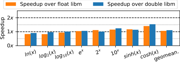


Figure 13 reports the speedup of RLibm-All’s functions over various mainstream libraries (glibc’s libm and Intel’s libm) and correctly rounded libraries (CR-LIBM and RLibm-32). Figure 13(a) presents the speedup of RLibm-All’s FP functions over glibc’s float functions (left bar in each cluster) and double functions (right bar in each cluster). On average, RLibm-All’s FP functions are and faster than glibc’s float and double functions, respectively. Figure 13(b) presents the speedup of RLibm-All’s FP functions over Intel’s float functions (left bar in each cluster) and double functions (right bar in each cluster). On average, RLibm-All has and speedup over Intel’s float and double functions, respectively. Figure 13(c) presents the speedup of RLibm-All’s FP functions over CR-LIBM functions. On average, RLibm-All has speedup over CR-LIBM functions. In contrast to RLibm-All, glibc’s libm, Intel’s libm, and CR-LIBM do not produce correct results for all inputs when used for a 32-bit float type.
Figure 13(d) presents the speedup of RLibm-All’s FP functions over RLibm-32’s functions in producing 32-bit float values rounded with the rounding mode. On average, RLibm-All is almost as fast as RLibm-32 (i.e., 2% slower than RLibm-32). RLibm-All creates polynomial approximations for a 34-bit FP representation, which is the main reason for this small performance slowdown. Notably, RLibm-All experiences roughly a 12% slowdown with when compared to RLibm-32. When an input is near , exhibits a linear behavior and produces correctly rounded float values with the rounding mode. RLibm-32 uses this property by simply returning for inputs near . In contrast, RLibm-All performs significantly more computation to ensure that it produces a value within the odd interval. Unlike RLibm-32 that produces correct results for a single representation with the mode, RLibm-All produces correct results for all inputs for multiple representations and all the standard rounding modes.
7. Related Work
Seminal research over multiple decades has advanced the state-of-the-art for creating polynomial approximations (Jeannerod et al. 2011; Bui and Tahar 1999; Ziv 1991; Daramy et al. 2003; Fousse et al. 2007; Muller 2005; Trefethen 2012; Remes 1934). Important advances in range reduction has made such approximation feasible (Tang 1990; Tang 1991; Tang 1989; Story and Ping Tak Peter Tang 1999; Cody and Waite 1980; Boldo et al. 2009). Simultaneously, there are verification efforts to prove bounds for math libraries (Harrison 2009; Harrison 1997a; Harrison 1997b; Sawada 2002; Lee et al. 2017) and repair individual outputs of math libraries (Yi et al. 2019; Zou et al. 2019). The comprehensive book on elementary functions provides detailed information on prior work (Muller 2005).
We restrict our comparison to prior work that is closely related to our work. As a correctly rounded elementary function is recommended by the IEEE standard and enables portability, a number of correctly rounded math libraries have been developed (Ziv 1991; Daramy et al. 2003; Lim et al. 2021; Lim et al. 2020; Lim and Nagarakatte 2021a). They are restricted to a specific representation and a rounding mode.
CR-LIBM (Daramy et al. 2003; Lefèvre et al. 1998) is a correctly rounded collection of elementary functions for double precision. It was developed using Sollya (Chevillard et al. 2010), which is a tool and a library for developing FP code. Sollya can generate polynomials of degree with coefficients in a representation used for the implementation () that has the minimum infinity norm (Brisebarre and Chevillard 2007). Sollya uses a modified Remez algorithm to produce polynomials. It also computes and proves the error bound on the polynomial evaluation using interval arithmetic (Chevillard and Lauter 2007; Chevillard et al. 2011). Metalibm (Kupriianova and Lauter 2014; Brunie et al. 2015) is a customization infrastructure also built using Sollya. MetaLibm is able to automatically identify range reduction and domain splitting techniques for some transcendental functions. It has been used to trade-off correctness and performance while approximating elementary functions for float and double precision types.
A modified Remez algorithm has also been used to generate polynomials that minimizes the infinity norm compared to an ideal elementary function (Arzelier et al. 2019). It can be useful for generating correctly rounded results for a specific precision and a rounding mode when range reduction is not necessary.
This paper builds on our prior work in the RLibm project (Lim et al. 2021; Lim et al. 2020; Lim and Nagarakatte 2021a; Lim and Nagarakatte 2021d; Lim 2021) that creates polynomials using the correctly rounded value rather than the real value of the elementary function. Like the RLibm project, we structure the problem of generating polynomials as an LP problem. We also use RLibm’s range reduction strategies. The RLibm project has generated correctly rounded libraries with the commonly used mode for multiple types: bfloat16, posit16, 32-bit float, and posit32. However, it is necessary to create individual polynomial approximation for each representation with each rounding mode with the RLibm project to avoid double rounding errors. In contrast, this paper shows that by generating polynomial approximations for with the round-to-odd mode, we can create a single polynomial approximation that works for multiple representations with multiple rounding modes.
8. Conclusion
This paper proposes a novel method to generate a single polynomial approximation that produces correctly rounded results for multiple representations and rounding modes. The key idea is to create a polynomial approximation that produces the correctly rounded result for with the round-to-odd mode when the goal is to generate correct results for , where , with all rounding modes. We address the issue of singletons while generating polynomials that approximate the correctly rounded result with the round-to-odd mode. We provide the first correctly rounded implementations of elementary functions for multiple representations. We believe that our results make a strong case for mandating correctly rounded results at least with any representation that has fewer than or equal to 32-bits.
Acknowledgements.
We thank John Gustafson for his inputs on the Minefield method and the posit representation. This material is based upon work supported in part by the Sponsor National Science Foundation http://dx.doi.org/10.13039/100000001 under Grant No. Grant #1908798, Grant No. Grant #1917897, and Grant No. Grant #2110861. Any opinions, findings, and conclusions or recommendations expressed in this material are those of the authors and do not necessarily reflect the views of the National Science Foundation.References
- (1)
- Aigner and Ziegler (2009) Martin Aigner and Gnter M. Ziegler. 2009. Proofs from THE BOOK (4th ed.). Springer Publishing Company, Incorporated.
- Arzelier et al. (2019) Denis Arzelier, Florent Bréhard, and Mioara Joldes. 2019. Exchange Algorithm for Evaluation and Approximation Error-Optimized Polynomials. In 2019 IEEE 26th Symposium on Computer Arithmetic (ARITH). 30–37. https://doi.org/10.1109/ARITH.2019.00014
- Baker (1975) Alan Baker. 1975. Transcendental Number Theory. Cambridge University Press.
- Boldo et al. (2009) Sylvie Boldo, Marc Daumas, and Ren-Cang Li. 2009. Formally Verified Argument Reduction with a Fused Multiply-Add. In IEEE Transactions on Computers, Vol. 58. 1139–1145. https://doi.org/10.1109/TC.2008.216
- Boldo and Melquiond (2005) Sylvie Boldo and Guillaume Melquiond. 2005. When double rounding is odd. In 17th IMACS World Congress. Paris, France, 11 pages.
- Boldo and Melquiond (2008) Sylvie Boldo and Guillaume Melquiond. 2008. Emulation of a FMA and Correctly Rounded Sums: Proved Algorithms Using Rounding to Odd. IEEE Transations on Computing 57, 4 (April 2008), 462–471. https://doi.org/10.1109/TC.2007.70819
- Borwein and Erdelyi (1995) Peter Borwein and Tamas Erdelyi. 1995. Polynomials and Polynomial Inequalities. Springer New York. https://doi.org/10.1007/978-1-4612-0793-1
- Brisebarre and Chevillard (2007) Nicolas Brisebarre and Sylvvain Chevillard. 2007. Efficient polynomial L-approximations. In 18th IEEE Symposium on Computer Arithmetic (ARITH ’07). https://doi.org/10.1109/ARITH.2007.17
- Brunie et al. (2015) Nicolas Brunie, Florent de Dinechin, Olga Kupriianova, and Christoph Lauter. 2015. Code Generators for Mathematical Functions. In 2015 IEEE 22nd Symposium on Computer Arithmetic. 66–73. https://doi.org/10.1109/ARITH.2015.22
- Bui and Tahar (1999) Hung Tien Bui and Sofiene Tahar. 1999. Design and synthesis of an IEEE-754 exponential function. In Engineering Solutions for the Next Millennium. 1999 IEEE Canadian Conference on Electrical and Computer Engineering, Vol. 1. 450–455 vol.1. https://doi.org/10.1109/CCECE.1999.807240
- Chevillard et al. (2011) Sylvain Chevillard, John Harrison, Mioara Joldes, and Christoph Lauter. 2011. Efficient and accurate computation of upper bounds of approximation errors. In Theoretical Computer Science, Vol. 412. https://doi.org/10.1016/j.tcs.2010.11.052
- Chevillard et al. (2010) Sylvain Chevillard, Mioara Joldes, and Christoph Lauter. 2010. Sollya: An Environment for the Development of Numerical Codes. In Mathematical Software - ICMS 2010 (Lecture Notes in Computer Science, Vol. 6327). Springer, Heidelberg, Germany, 28–31. https://doi.org/10.1007/978-3-642-15582-6_5
- Chevillard and Lauter (2007) Sylvain Chevillard and Christopher Lauter. 2007. A Certified Infinite Norm for the Implementation of Elementary Functions. In Seventh International Conference on Quality Software (QSIC 2007). 153–160. https://doi.org/10.1109/QSIC.2007.4385491
- Cody and Waite (1980) William J Cody and William M Waite. 1980. Software manual for the elementary functions. Prentice-Hall, Englewood Cliffs, NJ. https://doi.org/10.1137/1024023
- Cohn (1974) P. M. (Paul Moritz) Cohn. 1974. Algebra [by] P. M. Cohn. Wiley, London.
- Daramy et al. (2003) Catherine Daramy, David Defour, Florent Dinechin, and Jean-Michel Muller. 2003. CR-LIBM: A correctly rounded elementary function library. In Proceedings of SPIE Vol. 5205: Advanced Signal Processing Algorithms, Architectures, and Implementations XIII, Vol. 5205. https://doi.org/10.1117/12.505591
- Daramy-Loirat et al. (2006) Catherine Daramy-Loirat, David Defour, Florent de Dinechin, Matthieu Gallet, Nicolas Gast, Christoph Lauter, and Jean-Michel Muller. 2006. CR-LIBM A library of correctly rounded elementary functions in double-precision. Research Report. Laboratoire de l’Informatique du Parallélisme. https://hal-ens-lyon.archives-ouvertes.fr/ensl-01529804
- Fousse et al. (2007) Laurent Fousse, Guillaume Hanrot, Vincent Lefèvre, Patrick Pélissier, and Paul Zimmermann. 2007. MPFR: A Multiple-precision Binary Floating-point Library with Correct Rounding. ACM Trans. Math. Software 33, 2, Article 13 (June 2007). https://doi.org/10.1145/1236463.1236468
- Gleixner et al. (2012) Ambros M. Gleixner, Daniel E. Steffy, and Kati Wolter. 2012. Improving the Accuracy of Linear Programming Solvers with Iterative Refinement. In Proceedings of the 37th International Symposium on Symbolic and Algebraic Computation (Grenoble, France) (ISSAC ’12). Association for Computing Machinery, New York, NY, USA, 187–194. https://doi.org/10.1145/2442829.2442858
- Goldberg (1991) David Goldberg. 1991. What Every Computer Scientist Should Know About Floating-point Arithmetic. In ACM Computing Surveys, Vol. 23. ACM, New York, NY, USA, 5–48. https://doi.org/10.1145/103162.103163
- Gustafson and Yonemoto (2017) John Gustafson and Isaac Yonemoto. 2017. Beating Floating Point at Its Own Game: Posit Arithmetic. Supercomputing Frontiers and Innovations: an International Journal 4, 2 (June 2017), 71–86. https://doi.org/10.14529/jsfi170206
- Harrison (1997a) John Harrison. 1997a. Floating point verification in HOL light: The exponential function. In Algebraic Methodology and Software Technology, Michael Johnson (Ed.). Springer Berlin Heidelberg, Berlin, Heidelberg, 246–260. https://doi.org/10.1007/BFb0000475
- Harrison (1997b) John Harrison. 1997b. Verifying the Accuracy of Polynomial Approximations in HOL. In International Conference on Theorem Proving in Higher Order Logics. https://doi.org/10.1007/BFb0028391
- Harrison (2009) John Harrison. 2009. HOL Light: An Overview. In Proceedings of the 22nd International Conference on Theorem Proving in Higher Order Logics, TPHOLs 2009 (Lecture Notes in Computer Science, Vol. 5674), Stefan Berghofer, Tobias Nipkow, Christian Urban, and Makarius Wenzel (Eds.). Springer-Verlag, Munich, Germany, 60–66. https://doi.org/10.1007/978-3-642-03359-9_4
- Jeannerod et al. (2011) Claude-Pierre Jeannerod, Hervé Knochel, Christophe Monat, and Guillaume Revy. 2011. Computing Floating-Point Square Roots via Bivariate Polynomial Evaluation. IEEE Trans. Comput. 60. https://doi.org/10.1109/TC.2010.152
- Johnson (2018) Jeff Johnson. 2018. Rethinking floating point for deep learning. arXiv:1811.01721
- Kalamkar et al. (2019) Dhiraj D. Kalamkar, Dheevatsa Mudigere, Naveen Mellempudi, Dipankar Das, Kunal Banerjee, Sasikanth Avancha, Dharma Teja Vooturi, Nataraj Jammalamadaka, Jianyu Huang, Hector Yuen, Jiyan Yang, Jongsoo Park, Alexander Heinecke, Evangelos Georganas, Sudarshan Srinivasan, Abhisek Kundu, Misha Smelyanskiy, Bharat Kaul, and Pradeep Dubey. 2019. A Study of BFLOAT16 for Deep Learning Training. arXiv:1905.12322
- Köster et al. (2017) Urs Köster, Tristan Webb, Xin Wang, Marcel Nassar, Arjun K. Bansal, William Constable, Oguz Elibol, Stewart Hall, Luke Hornof, Amir Khosrowshahi, Carey Kloss, Ruby J. Pai, and Naveen Rao. 2017. Flexpoint: An Adaptive Numerical Format for Efficient Training of Deep Neural Networks. In Advances in Neural Information Processing Systems, Vol. abs/1711.02213.
- Kupriianova and Lauter (2014) Olga Kupriianova and Christoph Lauter. 2014. Metalibm: A Mathematical Functions Code Generator. In 4th International Congress on Mathematical Software. https://doi.org/10.1007/978-3-662-44199-2_106
- Lee et al. (2017) Wonyeol Lee, Rahul Sharma, and Alex Aiken. 2017. On Automatically Proving the Correctness of Math.h Implementations. Proceedings of the ACM on Programming Languages 2, POPL, Article 47 (Dec. 2017), 32 pages. https://doi.org/10.1145/3158135
- Lefèvre et al. (1998) Vincent Lefèvre, Jean-Michel Muller, and Arnaud Tisserand. 1998. Toward correctly rounded transcendentals. IEEE Trans. Comput. 47, 11 (1998), 1235–1243. https://doi.org/10.1109/12.736435
- Lim (2021) Jay Lim. 2021. Novel Polynomial Approximation Methods for Generating Correctly Rounded Elementary Functions. Ph.D. Dissertation. Rutgers University.
- Lim et al. (2020) Jay P. Lim, Mridul Aanjaneya, John Gustafson, and Santosh Nagarakatte. 2020. A Novel Approach to Generate Correctly Rounded Math Libraries for New Floating Point Representations. arXiv:2007.05344 Rutgers Department of Computer Science Technical Report DCS-TR-753.
- Lim et al. (2021) Jay P. Lim, Mridul Aanjaneya, John Gustafson, and Santosh Nagarakatte. 2021. An Approach to Generate Correctly Rounded Math Libraries for New Floating Point Variants. Proceedings of the ACM on Programming Languages 6, POPL, Article 29 (Jan. 2021), 30 pages. https://doi.org/10.1145/3434310
- Lim and Nagarakatte (2021a) Jay P. Lim and Santosh Nagarakatte. 2021a. High Performance Correctly Rounded Math Libraries for 32-bit Floating Point Representations. In 42nd ACM SIGPLAN Conference on Programming Language Design and Implementation (PLDI’21). https://doi.org/10.1145/3453483.3454049
- Lim and Nagarakatte (2021b) Jay P Lim and Santosh Nagarakatte. 2021b. RLIBM-32: High Performance Correctly Rounded Math Libraries for 32-bit Floating Point Representations. arXiv:2104.04043 Rutgers Department of Computer Science Technical Report DCS-TR-754.
- Lim and Nagarakatte (2021c) Jay P. Lim and Santosh Nagarakatte. 2021c. RLibm-all. https://github.com/rutgers-apl/rlibm-all
- Lim and Nagarakatte (2021d) Jay P. Lim and Santosh Nagarakatte. 2021d. RLIBM-ALL: A Novel Polynomial Approximation Method to Produce Correctly Rounded Results for Multiple Representations and Rounding Modes. arXiv:2108.06756 [abs] Rutgers Department of Computer Science Technical Report DCS-TR-757.
- Muller (2005) Jean-Michel Muller. 2005. Elementary Functions: Algorithms and Implementation. Birkhauser. https://doi.org/10.1007/978-1-4899-7983-4
- Niven (1956) Ivan Niven. 1956. Irrational Numbers. Mathematical Association of America.
- NVIDIA (2020) NVIDIA. 2020. TensorFloat-32 in the A100 GPU Accelerates AI Training, HPC up to 20x. https://blogs.nvidia.com/blog/2020/05/14/tensorfloat-32-precision-format/
- Remes (1934) Eugene Remes. 1934. Sur un procédé convergent d’approximations successives pour déterminer les polynômes d’approximation. Comptes rendus de l’Académie des Sciences 198 (1934), 2063–2065.
- Rouhani et al. (2020) Bita Rouhani, Daniel Lo, Ritchie Zhao, Ming Liu, Jeremy Fowers, Kalin Ovtcharov, Anna Vinogradsky, Sarah Massengill, Lita Yang, Ray Bittner, Alessandro Forin, Haishan Zhu, Taesik Na, Prerak Patel, Shuai Che, Lok Chand Koppaka, Xia Song, Subhojit Som, Kaustav Das, Saurabh Tiwary, Steve Reinhardt, Sitaram Lanka, Eric Chung, and Doug Burger. 2020. Pushing the Limits of Narrow Precision Inferencing at Cloud Scale with Microsoft Floating Point. In The Thirty-fourth Annual Conference on Neural Information Processing Systems. ACM.
- Sawada (2002) Jun Sawada. 2002. Formal verification of divide and square root algorithms using series calculation. In 3rd International Workshop on the ACL2 Theorem Prover and its Applications.
- Story and Ping Tak Peter Tang (1999) Shane Story and Ping Tak Peter Tang. 1999. New algorithms for improved transcendental functions on IA-64. In Proceedings 14th IEEE Symposium on Computer Arithmetic. 4–11. https://doi.org/10.1109/ARITH.1999.762822
- Tagliavini et al. (2018) Giuseppe Tagliavini, Stefan Mach, Davide Rossi, Andrea Marongiu, and Luca Benin. 2018. A transprecision floating-point platform for ultra-low power computing. In 2018 Design, Automation Test in Europe Conference Exhibition (DATE). 1051–1056. https://doi.org/10.23919/DATE.2018.8342167
- Tang (1989) Ping-Tak Peter Tang. 1989. Table-Driven Implementation of the Exponential Function in IEEE Floating-Point Arithmetic. ACM Trans. Math. Software 15, 2 (June 1989), 144–157. https://doi.org/10.1145/63522.214389
- Tang (1990) Ping-Tak Peter Tang. 1990. Table-Driven Implementation of the Logarithm Function in IEEE Floating-Point Arithmetic. ACM Trans. Math. Software 16, 4 (Dec. 1990), 378–400. https://doi.org/10.1145/98267.98294
- Tang (1991) P. T. P. Tang. 1991. Table-lookup algorithms for elementary functions and their error analysis. In [1991] Proceedings 10th IEEE Symposium on Computer Arithmetic. 232–236. https://doi.org/10.1109/ARITH.1991.145565
- Trefethen (2012) Lloyd N. Trefethen. 2012. Approximation Theory and Approximation Practice (Other Titles in Applied Mathematics). Society for Industrial and Applied Mathematics, USA.
- Yi et al. (2019) Xin Yi, Liqian Chen, Xiaoguang Mao, and Tao Ji. 2019. Efficient Automated Repair of High Floating-Point Errors in Numerical Libraries. Proceedings of the ACM on Programming Languages 3, POPL, Article 56 (Jan. 2019), 29 pages. https://doi.org/10.1145/3290369
- Ziv (1991) Abraham Ziv. 1991. Fast Evaluation of Elementary Mathematical Functions with Correctly Rounded Last Bit. ACM Trans. Math. Software 17, 3 (Sept. 1991), 410–423. https://doi.org/10.1145/114697.116813
- Zou et al. (2019) Daming Zou, Muhan Zeng, Yingfei Xiong, Zhoulai Fu, Lu Zhang, and Zhendong Su. 2019. Detecting Floating-Point Errors via Atomic Conditions. Proceedings of the ACM on Programming Languages 4, POPL, Article 60 (Dec. 2019), 27 pages. https://doi.org/10.1145/3371128