Efficient Anytime CLF Reactive Planning System
for a Bipedal Robot on Undulating Terrain
Abstract
We propose and experimentally demonstrate a reactive planning system for bipedal robots on unexplored, challenging terrains. The system consists of a low-frequency planning thread (5 Hz) to find an asymptotically optimal path and a high-frequency reactive thread (300 Hz) to accommodate robot deviation. The planning thread includes: a multi-layer local map to compute traversability for the robot on the terrain; an anytime omnidirectional Control Lyapunov Function (CLF) for use with a Rapidly Exploring Random Tree Star (RRT*) that generates a vector field for specifying motion between nodes; a sub-goal finder when the final goal is outside of the current map; and a finite-state machine to handle high-level mission decisions. The system also includes a reactive thread to obviate the non-smooth motions that arise with traditional RRT* algorithms when performing path following. The reactive thread copes with robot deviation while eliminating non-smooth motions via a vector field (defined by a closed-loop feedback policy) that provides real-time control commands to the robot’s gait controller as a function of instantaneous robot pose. The system is evaluated on various challenging outdoor terrains and cluttered indoor scenes in both simulation and experiment on Cassie Blue, a bipedal robot with 20 degrees of freedom. All implementations are coded in C++ with the Robot Operating System (ROS) and are available at https://github.com/UMich-BipedLab/CLF_reactive_planning_system.
I Introduction


Motion planning as a central component for autonomous navigation has been extensively studied over the last few decades. Algorithms such as , , and their variants focus on finding an (asymptotically) optimal path as computationally efficiently as possible[1, 2, 3, 4, 5, 6, 7, 8, 9]. The application of these algorithms relies on designing a control policy to track the planned path, resulting in waypoint following or pathway tracking. In turn, the tracking of path segments (between waypoints) leads to non-smooth motion of the actual robot, due to abrupt acceleration or heading changes when transitioning between waypoints/pathways.
This paper seeks to develop a reactive planning system for bipedal robots on unexplored, unmapped, challenging terrains and to provide high-rate (directional) velocity and heading commands to be realized by the robot’s low-level feedback-control gait-generation algorithm. For this application, the non-smooth aspects of the planned motions arising from waypoints/pathways transitions are detrimental to stability of the overall system.
Several approaches have been developed to address the non-smooth aspects of paths produced by motion planning, such as reactive motion planning [10, 11, 12, 13, 14, 15, 16, 17, 18] and feedback motion planning [19, 20, 21]. Fundamentally, these approaches replace paths to be followed with smooth vector fields whose solutions guide the robot’s evolution in its configuration space.
We are inspired by the work of [20, 21], which proposes a Control Lyapunov Function (CLF) to realize reactive planning for a non-holonomic differential-drive wheeled robot. While their underlying model is not applicable to a Cassie bipedal robot, their basic concept is applicable. As part of our work, we design an appropriate CLF for robots capable of walking in any direction with any orientation. Moreover, we take into account features specific to bipeds, such as the limited lateral leg motion that renders lateral walking more laborious than sagittal plane walking.
The feedback motion planning algorithm in [20, 21] has not yet been evaluated on hardware. In general, there is a significant chasm between a planning algorithm and autonomous navigation on real robots. Most planning algorithms assume not only that a fully-explored, noise-free, perfect map is given but also that the robot’s destination will always lie within this map. Moreover, the algorithms also assume a perfect robot pose and a perfect robot with ideal actuators that can execute an arbitrary trajectory. These assumptions are not practical. Therefore, utilizing a planning algorithm for autonomous navigation with real robots remains challenging. We propose and demonstrate experimentally an autonomous navigation system for a Cassie bipedal robot that is able to handle a noisy map in real-time, a distant goal that may not be in the initial map when the user decides where to send the robot, and importantly, a means to smoothly handle robot deviation. Additionally, a rudimentary finite-state machine is integrated to handle actions such as where to turn at intersections.
II Related Work and Contributions
Motion planning, an essential component of robot autonomy, has been an active area of research for multiple decades with an accompanying rich literature. In this section, we review several types of planning algorithms and summarize our main contributions.
II-A Sampling-Based Motion Planning
Rapidly exploring Tree (RRT)[1] stands out for its low complexity and high efficiency in exploring unknown configuration spaces. Its asymptotically optimal version — [5] — has also gained much attention and has contributed greatly to the spread of the RRT family. RRT, , and variations on the basic algorithms, generate a collision-free path comprised of piece-wise linear paths between discrete poses of the robot [1, 2, 3, 4, 5, 6, 7, 8, 9, 22, 23]. However, abrupt (non-differentiable) transitions between waypoints/pathways are an inherent issue with this family of planning algorithms and in addition, the generated trajectories do not account for control constraints. Therefore, to ensure the produced trajectories are feasible, additional expensive computations such as trajectory smoothing or optimization are often involved. A great deal of attention has been directed to this area, resulting in versions of [24, 25, 26, 27, 28, 29] that utilize different smoothing techniques or steering functions.
Trajectory smoothing (B-spines, Dubins, or other parametric curves) is often designed independently of robot dynamics[30, 31, 32], which can lead to unbounded turning rate, acceleration, or jerk. Therefore, additional computations are necessary to validate the resulting smoothed trajectory. Furthermore, these methods are often ambiguous about how they treat robot deviations about the planned path and in the end provide open-loop control laws for tracking.
II-B Reactive Planning
Reactive planning contributes another significant concept to the motion planning literature [10, 11, 12, 13, 14, 15, 16, 17, 18], namely potential fields. The method of reactive planning controls the motion of a robot by covering the configuration space with a potential field, creating a single attractive equilibrium around the target point and repulsive actions around obstacles. In other words, the reactive planning replaces the concept of trajectory with that of a vector field arising as the gradient of a potential function. The method of potential fields seems to address all the issues raised in Sec. II-A for sampling-based methods. However, most of the experimental work has been carried out on flat ground and it is unclear how extensions to undulating terrain can be performed. Maybe the biggest drawback for real-time applications is that these algorithms require a complete map to construct a potential field.
The concept of combining sampling-based algorithms with reactive planning was developed in [19, 20, 21], which not only provides a feasible path to follow from , but also a smooth feedback control law that instantaneously replans a path to the next goal as the robot deviates due to model imperfections in the robot’s hardware or terrain. The feedback laws greatly ameliorate the issue of non-smooth paths. The feedback motion planning in [19] is based on a family of CLFs designed via linearization of the robot’s model around a sufficiently large set of points in the robot’s state space, LQR, and Sum of Squares (SoS), whereas the feedback motion planning of [20, 21] uses a single CLF and varies the associated equilibrium to set sub-goal poses.
The feedback motion planning of [20, 21] is a form of non-holonomic for differential-drive wheeled robots, where a CLF is utilized as the steering function in the algorithm and results in a system where robot control and motion planning are tightly coupled. This method is closest to ours. The CLF in [20, 21] is designed for differential-drive wheeled robots and hence is not suitable for bipeds, see Sec. III-A. Additionally, their version of assumes the robot is on flat ground and thus is not appropriate for undulating terrains. To date, the work has not been evaluated on hardware.
In this paper, we propose a CLF that is suitable for bipeds or omnidirectional robots (Sec. III) and utilize the proposed CLF in the algorithm; see Sec. IV. We integrate the omnidirectional into a full reactive planning system consisting of both a planning thread and a reactive thread. The planning thread includes a multi-layer, robot-centric local map, an anytime omnidirectional CLF , a sub-goal finder, and a finite-state machine. The reactive thread utilizes the CLF as a reactive planner to handle robot deviations; see Sec. V.
II-C Contributions
In particular, the present work has the following contributions:
- 1.
We propose a novel smooth Control Lyapunov Function (CLF) with a closed-form solution to the feedback controller for omnidirectional robots. The CLF is designed such that when a goal is far from the robot position, the CLF controls the robot orientation to align with the goal while moving toward the goal. On the other hand, the robot walks to the goal disregarding its orientation if the goal is close. Additionally, we study the behaviors of the CLF under different initial conditions and parameters.
- 2.
We define a closed-form distance measure from a pose (position and orientation) to a target position for omnidirectional robots under a pose-centric polar coordinate. This distance metric nicely captures inherent features of Cassie-series robots, such as the low-cost of longitudinal movement and high-cost of lateral movement.
- 3.
We utilize the proposed CLF and the distance measure to form a new variation of (omnidirectional CLF ) to tackle undulating terrains, in which both distance and traversability are included in the cost to solve the optimal path problem. Moreover, as in [20], the optimal path is realized as a sequence of subgoals that are connected by integral curves of a set of vector fields, thereby providing reactive planning: in response to a disturbance, each vector field associated with the optimal path automatically guides the robot to a subgoal along a new integral curve of the vector field.
- 4.
We integrate all the above components together as a reactive planning system for challenging terrains/cluttered indoor environments. It contains a planning thread to guide Cassie to walk in highly traversable areas toward a distant goal on the basis of a multi-layer map being built in real-time and a reactive thread to handle robot deviation via a closed-loop feedback control instead of a commonly used waypoint-following or path-tracking strategy.
We evaluate the reactive planning system by performing three types of experiments: 1) A simplified biped pendulum model (inputs are piece-wise constant, similar to Cassie-series robots) navigates various synthetic, noisy, challenging outdoor terrains and cluttered indoor scenes. The system guides the robot to its goals in various scenes, both indoors and outdoors, with or without obstacles. The system also guides the robot to completion of several high-level missions, such as turning left at every intersection. 2) To verify that the outputs of the control commands are feasible for Cassie-series robots, the system gives commands to a Cassie whole-body dynamic simulator [33], which simulates 20 degrees of freedom (DoF) of Cassie in Matlab Simmechanics on a 3D terrain. 3) Lastly, the reactive planning system successfully allows Cassie Blue to complete several indoor and outdoor missions: a) walking in corridors and avoiding furniture in the Ford Robotics Building (FRB) at the University of Michigan; b) turning left when detected intersections of corridors and return to its initial position in FRB; and c) traversing parts of the Wave Field on the North campus of the University of Michigan, as shown in Fig 1.
The videos of the autonomy experiments can be found at [34]. All of the simulated environments, the experimental data, and the C++ implementations for the reactive planning system are made available at https://github.com/UMich-BipedLab/CLF_reactive_planning_system[35].
The remainder of this paper is organized as follows. Section III constructs the new CLF for bipeds and omnidirectional robots. The omnidirectional CLF is introduced in Sec. IV. Section V integrates all the above components as a reactive planning system. Simulated and experimental evaluations of the proposed reactive system is presented in Sec. VI. Finally, Sec. VII concludes the paper and provides suggestions for future work.


III Construction of a Control Lyapunov Function
This section describes the reasons for creating a new CLF function, the construction of the CLF, and an analysis of its parameters.
III-A Deficiency of Existing CLFs
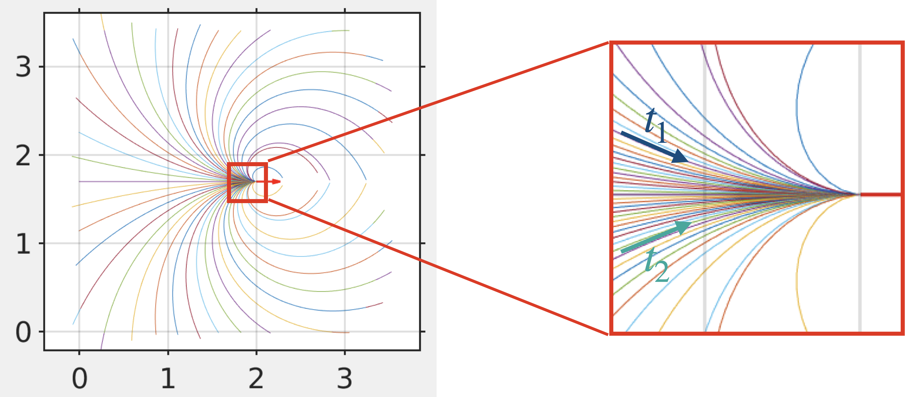
The existing 2D CLF planners [21, 20] are designed for differentially driven non-holonomically constrained robots, whose dynamics and control laws are inappropriate for bipedal robots. Like most robot models, this work assumes that the robot is able to continuously change its velocity and heading. However, this is not possible for underactuated bipeds such as Cassie Blue. According to the ALIP model used for low-level feedback control of Cassie Blue [36, 37, 38, 39, 40], the heading angle and the longitudinal and lateral velocity commands can only be updated at the initiation of a step and not within a step. In other words, bipedal robots such as Cassie are not able to update their control commands during the swing phase and will execute the received control commands for the entire swing phase. When piece-wise constant commands are applied to the existing 2D CLF of [21, 20], built around a Dubins car model, the closed-loop system will oscillate about the discrete heading directions as the robot approaches the goal pose, as explained in Fig. 2. This oscillation is undesirable as it can affect the robot’s balance.
With a Dubins car model as used in [21, 20], the linear velocity is always aligned with the heading angle of the vehicle, and hence this is also true as the vehicle approaches an equilibrium pose. Consequently, a CLF for a target position must also include a target heading, therefore, a target pose. The vehicle must steer and align itself as it approaches the target. Cassie Blue, on the other hand, similar to an omnidirectional robot, is able to move laterally with zero forward velocity, which allows the robot to start with an arbitrary pose and arrive at a goal position with an arbitrary heading (i.e., start with a pose and end with a position). Lateral walking, however, requires more effort due to the limited workspace of the lateral hip joints on the robot and this should be taken into account when designing a CLF.
To avoid undesirable oscillating movement and account for lateral walking, a new candidate CLF is designed on the basis of an appropriate kinematics model for underactuated bipeds and other omnidirectional robots.
III-B State Representation
As mentioned in Sec. III, Cassie Blue is able to walk in any direction. Therefore, we model Cassie Blue as an omnidirectional robot and reduce it to a directional point mass. We will account for the increased effort required to walk laterally when we design the CLF.
Denote the robot pose and the goal position in the world frame. Let be the state of an omnidirectional robot represented in a robot pose-centric polar coordinate:
| (1) |
where and is the angle between the heading angle of the robot and the line of sight from the robot to the goal, as shown in Fig. 3.
Remark 1.
III-C Construction of Control Lyapunov Function
The kinematics of an omnidirectional robot is defined as
| (2) |
In the above expression, we view , and as control variables. Because the matrix
is negative definite (and hence invertible) for all , the model (2) is over actuated for .
Remark 2.
We next note that the change of control variables
allows us to feedback linearize the model to a pair of integrators
We note that for this model, any positive definite quadratic function is automatically a CLF. For later use, we note that for all ,
| (3) |
As mentioned in Sec. III, lateral walking is more expensive than longitudinal walking because movement in the lateral hip joint is limited. A candidate control Lyapunov function11 1 In polar coordinate, the function is positive definite in the sense that , and when , the angle is arbitrary or undefined. , in terms of the robot’s current pose and target (end) position, is defined as
| (4) |
where is a weight on the orientation and the role of will be described later. We next check that is a Control-Lyapunov function. The derivative of is
| (5) | ||||
The feedback
| (6) | ||||
results in
| (7) |
which is negative for all , , .
Remark 3.
From (6), it follows that for . Therefore, the manifolds
are invariant for the closed-loop system. From (7), the manifold is locally attractive for and repulsive for . By selecting , the repulsive invariant manifold can be placed outside the field of view (FoV) of Cassie, as shown in Fig. 6. In practice, a finite-state machine (FSM) is needed so that the robot will initially turn in place so that it starts with the goal located within the FoV of its sensor suite.
The next step is to set up an optimization such that the control variables satisfy (6) and take into account that walking sideways takes more effort than walking forward, for Cassie. Because the camera faces forward, walking backward is only selected if the robot is localized into an already built portion of the map.
III-D Closed-form Solution
Taking (3) as a constraint, we propose to select so as to keep small (limit lateral walking) by optimizing
| (8) |
The parameter allows us to penalize aggressive yaw motions , as will be illustrated in Sec. III-E. Plugging in the constraint (3), (8) leads to
A few algebraic calculations and the dropping of “constant terms” lead to
which implies that
. The final result is
| (9) |
and then
| (10) | ||||

| 10 | 1.2 | 1 | 1 | 5 | 0.1 | 10 |
III-E Qualitative Analysis of the Closed-loop Trajectories
The default parameters applied in this analysis are shown in Table. I. Figure 5 shows how the closed-loop trajectories vary as a function of heavy, medium, and light penalties on yaw motion, and three different initial distances from the target, with , the robot’s heading relative to the target, fixed at . We observe that with , the robot walks laterally to achieve the goal for all values of the penalty on yaw motion. With and , the robot aligns its heading to the target while walking to reduce its lateral movement, whereas with , it maintains its heading and combines lateral and longitudinal motion as needed to reach the goal.
Figure 6 shows how the closed-loop trajectories vary as a function the initial relative heading to the target, when starting at a fixed distance of m, and . As indicated in Table I, we are using , which yields FoV of . For relative heading “errors” less than , the robot aligns quickly to the target and longitudinal walking dominates. If quicker zeroing of the heading error is desired, a smaller value of could be used or the robot could turn in place before starting a new segment.

IV Omnidirectional CLF-
This section integrates the CLF proposed in Sec. III into the original algorithm. The resulting omnidirectional CLF provides feasible paths for (2) while (i) accounting for relative heading, (ii) the asymmetry in roles of target position and current pose induced by the CLF, and (iii) the fact that walking laterally is more challenging than walking in the longitudinal direction for robots such as Cassie.
IV-A Standard Algorithm
The original [3] is a sampling-base, incremental planner with guaranteed asymptotic optimality. In configuration space, grows a tree where leaves are states connected by edges of linear path segments with the minimal cost. Additionally, considers nearby nodes of a sample to choose the best parent node and to rewire the graph if shorter path is possible to guarantee asymptotic optimality.
IV-B Omnidirectional CLF- Algorithm
The omnidirectional CLF- differs from the original in four aspects. First, the distance between two nodes is defined by the CLF in (4), which takes relative heading into account. Second, the steering/extending functions use the closed-loop trajectories generated by (10) to define paths between nodes. Third, because the cost (4) between two nodes and is not symmetric (i.e, a different cost is assigned if node is the origin versus it is the target), a distinction must be made between near-to nodes and near-from nodes. The above three aspects are common to the CLF- variant introduced in [20, 21]. Finally, when connecting, exploring, and rewiring the tree, an additional term is added to the cost (4) to account for the relative ease or difficulty of traversing the path.
Our proposed modification is summarized below with notation that generally follows [4]. Let be the configuration space and let denote the obstacle region, which together define the free region for walking . The omnidirectional CLF solves the optimal path planning problem by growing a tree , where is a vertex set of poses connected by edges of feasible path segments. Briefly speaking, the proposed (Algorithm 1) explores the configuration space by random sampling and extending nodes to grow the tree (explore the configuration space), just as in the classic RRT[1]. Considering nearby nodes of a sample to choose the best parent node and rewiring the graph guarantee asymptotic optimality (Algorithm 2 and 3), as with the classic algorithm. As emphasized previously, a key difference lies in how the paths between vertices are generated.
IV-B1 Sampling
This step randomly samples a pose . To facilitate faster convergence and to find better paths, we use sampling with a goal bias, limited search space, and Gaussian sampling. For more details, see our implementation on GitHub [35].
IV-B2 Distance
The distance from node to node in the tree is defined by (4), which takes relative heading into account. Note that when computing the distance, is a pose and the heading of is ignored and only its values are used.
Remark 4.
As mentioned in Sec. III-C, the robot will rotate in place if the target point is outside the FoV. If rotating in place is laborious, one can also consider the following distance function:
| (11) |
where is defined in (4), is a positive constant, and corresponds to a repulsive point (i.e., ) in Remark 3.
IV-B3 Traversability of a path
Let be the current robot pose and denote the path22 2 The path is generated from the CLF in Sec. III. connecting and . We also denote as the elevation and the magnitude of the gradient at a point in a local map , see Sec. V-B. Finally, let be the cost of the path traversability, defined as
| (12) | ||||
where and are the corresponding positive coefficients.
Remark 5.
Traversability varies among different types of robots. Additional elements can be added as needed to account for different aspects for traversability computation.
IV-B4 Cost between Nodes
Let be the cost from to in the tree , defined as
| (13) |
where is the weight of traversability.
IV-B5 Nearby Nodes
Due to the use of the CLF function, the distinction between near-to nodes and near-from nodes is necessary.
| (14) | ||||
where is the absolute value, is the number of nodes in the tree , and with the constant and dimension of space ( in our case) [6] and is a positive constant. Similarly, the near-from nodes are determined by
| (15) | ||||
IV-B6 Nearest Node
Given a node , the tree , and the local map , the nearest node is any node in the tree where the cost from to is minimum.
IV-B7 Steering and Extending
The steering function generates a path segment that starts from and ends exactly at . The extending function extends the path from toward until is reached or the distance traveled is in which case it returns a new sample at the end of the extension.
ChooseParent()
IV-B8 Parent Choosing and Graph Rewiring
Choosing the best parent node (Algorithm 2) and rewiring the graph (Algorithm 3) guarantee asymptotic optimality. Let Cost be the cost from the root of the tree to the node . The parent of a node is determined by finding a node with smallest cost from the root to the node:
| (16) |
After a parent node is chosen, nearby nodes are rewired if shorter paths are found. In our experiments, we used the extending function for exploration, and the steering function to find the best parent node and to rewire the graph.
IV-B9 Collision Check
This step verifies whether a path lies within the obstacle-free region of the configuration space. Note that additional constraints, such as curvature bounds and minimum clearance, can also be examined in this step.
IV-B10 Node Insertion
Given the current tree and a node , this step inserts the node to and creates an edge from to .
Cost() c() Cost() then 3
V Reactive Planning System
The previous section provides a sparse set of paths from a robot’s initial location to a goal. The degree of optimality depends on how long the planning algorithm is run. A typical update rate may be 5 Hz for real-time applications. When the robot is perturbed off the nominal path, one is left with deciding how to reach the goal, say by tracking the nominal path with a PID controller. Important alternatives to this, called a high-frequency reactive planner or a feedback motion planner, were introduced in [10, 11, 12, 13, 14, 15, 16, 17, 18, 19]. A version based on the work of [20, 21] will be incorporated into our overall planning system. In addition, we take into account features in a local map.
V-A Elements of the Overall Planning System
The overall objective of the planner system is to replace the commonly used waypoint-following or path-tracking strategies with a family of closed-loop feedback control laws that steer the robot along a sequence of collision-free sub-goals leading to the final goal. In simple terms, as in [19, 20, 21], we populate the configuration space with a discrete set of feedback control laws that steer the robot from local chart about a sub-goal to the sub-goal itself. The collision free property is handled by the low-frequency planner at the current time. Others have used CBFs for this purpose [41, 42, 43, 44, 45, 46]. A finite-state machine (FSM) is integrated into the low-frequency planner to handle high-level mission requirements such as turning left at every intersection.
The planner assumes the initial robot pose, a final goal, and real-time map building are provided. It is assumed that the initial robot pose and final goal are initialized in an otherwise featureless metric map, with the robot’s initial pose as the origin. The featureless map is filled in by the real-time mapping package [47, 48, 49] based on collected LiDAR and/or camera data.

V-B Planning Thread
The planning thread deals with short-range planning (less than 20 meters) at a frequency of 5 to 10 Hz. It includes a robot-centric local map, our omnidirectional CLF- algorithm of Section III, cost computation, a sub-goal finder, and a finite-state machine.
V-B1 Robot-centric Local Map and Cost Computation
Figure 8(a) shows the robot-centric multi-layer local map (highlighted area), which crops a sub-map centered around the robot’s current position from the global map provided by the mapping algorithm. The local map computes additional useful information such as terrain slope (local gradient) which is useful for assigning cost. Moreover, other necessary operations for different experiment scenes such as applying the Bresenham algorithm [51] to remove walkable area behind glass walls can be computed in this step, see Sec. VI-D. Additionally, terrain information such as slopes and frictions can be sent to a terrain-aware low-level controller [50]. The computations with the local map are efficient compared to processing the full map.


V-B2 Anytime Omnidirectional CLF- Planner
The anytime feature is a direct result of using as a planner. The algorithm can be queried at anytime to provide a suboptimal path comprised of wayposes, which the CLF (4) turns into real-time feedback laws for anytime replanning.


V-B3 Sub-goal Finder and Finite-State Machine
Ideally, a global planner is present to guide the robot to a distant goal, which may not be viewable at the time of mission start [52]. In relatively simple situations such as that shown in Fig. 9 and Fig. 8(b), it is sufficient to complete many of short-term missions by positioning a sub-goal (green arrow) at the lowest cost (cost-to-come + cost-to-goal) on an arc (blue arrows) to guide the robot to the final goal. This sub-goal finder is also used as a finite-state machine to handle high-level missions such as making turn selections at intersections. In the future, the sub-goal finder will be replaced with a global planner.
V-C Reactive Thread
The work in [10, 11, 12, 13, 14, 15, 16, 17, 18] provided a significant alternative to the standard path tracking. Their high frequency reactive planners create a vector field on the configuration space whose integrals curves (i.e., solutions of the vector field) provide alternative paths to the goal. When the robot is perturbed, it immediately starts following the new path specified by the vector field, instead trying to asymptotically rejoin the original path. The vector field is in essence an instantaneous re-planner.
In the reactive planner of [11, 13], the vector field arises from the gradient of a potential function defined on the configuration space. Here, we use the solutions of the closed-loop system associated with the CLF in (4) to define alternative paths in the configuration space. In essence, our feedback functions (10) and (9) provide instantaneous re-planning of the control commands for the omnidirectional model (2). This reactive planner can be run at 300 Hz in real-time.
The reactive thread is a reactive planner, in which the motion of the robot is generated by a vector field that replies on a closed-loop feedback policy giving controller commands in real-time as a function of the instantaneous robot pose. In other words, the reactive planner utilizes the proposed Control Lyapunov Function described in Sec. III to adjust controller commands automatically when the robot deviates from the optimal path. This thread steers the robot to the optimal path at 300 Hz.
Remark 6.
The “timing” of Cassie’s foot placement is inherently event-driven and stochastic. Even though a step cycle may be planned for 300 ms, variations in the terrain and deviations of the robot’s joints from nominal conditions result in foot-ground contact being a random variable, with a mean of roughly 300 ms. Running the reactive planner at anything over 100 Hz essentially guarantees that Cassie’s gait controller, which runs at 2 kHz, is accepting the most up-to-date commands from the planner, even if a few messages are lost over UDP transmission.
VI Simulation and Experimental Results
The proposed reactive planning system integrates a local map, the omnidirectional CLF , and fast replanning from the reactive thread. We performed three types of evaluation of the reactive planning system.
VI-A Angular Linear Inverted Pendulum (ALIP) Robot with Simulated Challenging Outdoor Terrains and Indoor Cluttered Scenes
We first ran the reactive planning system on several synthetic environments, in which an ALIP robot model [37, 36] navigated several simulated noisy, patchy, challenging outdoor terrains as well as cluttered indoor scenes. The ALIP robot successfully reached all the goals in different scenes. We tested the system on more than 10 different environments, both indoor and outdoor with and without obstacles. Due to space limitations, we only show the results of six simulations in Fig 9; see our GitHub[35] for videos and more results.
Remark 7.
The ALIP robot[37, 36] takes piece-wise constant inputs from the reactive planning system. Let be the gravity, the robot’s center of mass height, and the time interval of a swing phase, respectively. The motion of an ALIP robot on the -axis is defined as
| (17) |
where is the center of mass (CoM) on the -axis of the robot, and . Similarly, the motion of the robot on the -axis can be defined.
Remark 8.
Even though a full global map is given in each simulation environment, only the information in the local map is given to the planning system at each timestamp. The path generated from omnidirectional is asymptotically optimal within the local map, for the given time window. It is emphasized that no global information is provided to the planner which is why the resulting trajectory from the initial point to the goal may not be the shortest path.
VI-B Validation of Control Command Feasibility via a Whole-body Cassie Simulator
To ensure the control commands from the reactive planning system are feasible for Cassie-series bipedal robots, we sent the commands via User Datagram Protocol (UDP) from ROS[53] C++ to Matlab-Simmechanics, which simulates a 20 DoF of Cassie, using footfalls on the specified terrain. The simulator then sent back the pose of the simulated Cassie robot to the planning system to plan for the optimal path via UDP. The planner system successfully took the simulated Cassie to the goal without falling, as shown in Fig. 10.

VI-C System Integration for Real-time Deployment
System integration is critical for real-time use. Figure 11 shows the integrated system, distribution, and frequency of each computation. In particular, the sensor calibrations are performed via[54, 55, 56, 57, 58, 59, 60, 61, 62, 63]. The invariant Extended Kalman Filter (InEKF)[64, 65] is used to estimate the state of Cassie Blue at 2 kHz. Images are segmented via MobileNets[66] and a LiDAR point cloud is projected back to the segmented image to produce a 3D segmented point cloud. The resulting point clouds are then utilized to build a multi-layer map (MLM) [47, 48, 49]. The reactive planning system then crops the MLM around the robot position to create a local map and performs several operations to acquire extra information, as described in Sec. V-B. Additionally, the reactive planner receives the robot poses from the InEKF at 300 Hz to adjust the control commands that guide the robot to the nominal sub-poses via the proposed CLF; see Sec. III and Sec. V-C. The control commands are then sent to Cassie Blue’s gait controller [36, 67, 68] via UDP.

VI-D Full Autonomy Experiments with Cassie Blue
We conducted several indoor and outdoor full autonomy experiments with Cassie Blue.
VI-D1 The Wave Field
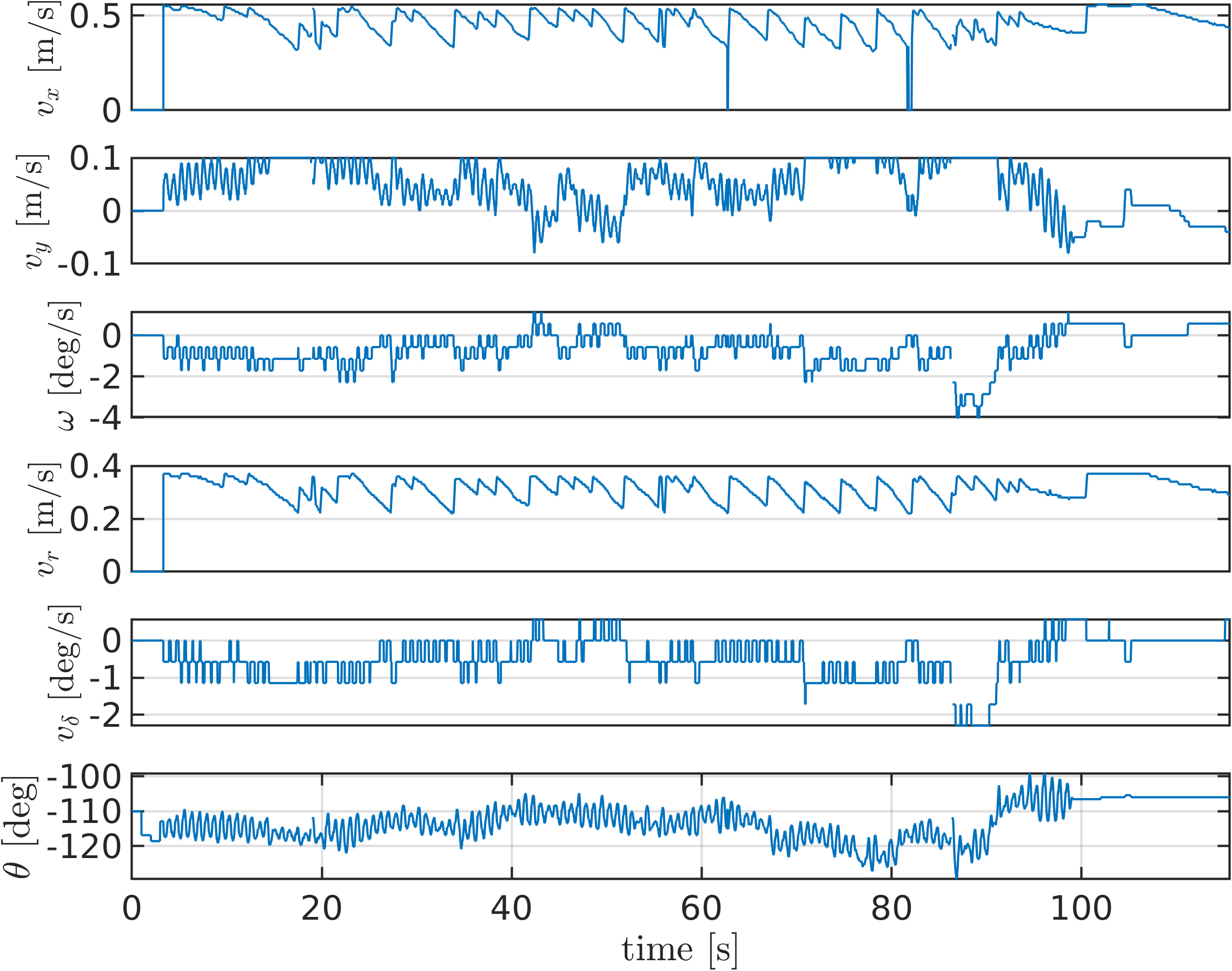
We achieved full autonomy with Cassie Blue on the Wave Field, located on the North campus of the University of Michigan, an earthen sculpture designed by Maya Lin [69]; see Fig. 12(a). The Wave Field consists of sinusoidal humps with a depth of approximately 1.5 m from the bottom of the valleys to the crest of the humps; there is a second sinusoidal pattern running orthogonal to the main pattern, which adds 25 cm ripples peak-to-peak even in the valleys. Figure 12(b) shows the top-view of the resulting trajectory of the reactive planning system. The planning system guided Cassie Blue to walk in the valley (the more traversable area), as shown in Fig. 12(c). The planning system navigated Cassie Blue around a hump that protrudes into one of the valleys, as shown in Fig. 12(d). Figure 13 shows the control commands sent to Cassie Blue. This experiment was presented in the Legged Robots Workshop at ICRA 2021; the video can be viewed at [70]. The video of the Wave Field experiment is uploaded and can be found at [34] and [35].


VI-D2 Turn left at detected intersections of corridors and avoid obstacles
We conducted two experiments of this type on the first floor of the Ford Robotics Building (FRB) at the University of Michigan. The experiments’ scenes consist of corridors and an open area cluttered with tables and couches, which are considered as obstacles, as shown in Fig. 14. To detect the intersections of the corridors, we group walkable segments within a ring around Cassie Blue via the single-linkage agglomerative hierarchical clustering algorithm33 3 We chose this clustering algorithm because the number of clusters is unknown. Therefore, algorithms like K-Means Clustering [71] cannot be used.[72]. Subsequently, Cassie Blue makes a left turn at the detected intersection. After exiting the corridors, the robot reaches an open area cluttered with furniture and performs obstacle avoidance. Under the proposed reactive planning system, Cassie Blue completed the experiments without falling or colliding with obstacles. The total distance traveled was about 80 meters. The experiment videos can be viewed at [73] and [35].


VI-D3 Turn right at detected intersections of corridors and return to the initial position
This experiment was conducted on the second floor of the FRB and the experiment scene contains four long corridors with glass walls. Some of the LiDAR beams penetrated glass a certain points along the corridors, causing the mapping algorithm to consider area behind the glass walls as free and walkable. We applied the Bresenham line algorithm [51] to remove the walkable area behind the glass walls. The computation of the Bresenham algorithm is not expensive because it is only applied within the local map, mentioned in Sec. V-B. The proposed reactive planning system successfully guided Cassie Blue back to its initial position, as shown in Fig. 15. The total distance traveled was about 200 meters. The experiment videos can be viewed at [74] and [35].
VI-E Experiment Discussion
In the two indoor experiments, Cassie exhibited a walk-and-stop motion. Where does it come from? As mentioned in Sec. V, the planning threading runs at 5 Hz. At the -th update, there will be an optimal path , comprised of a number of way-poses connected by CLFs. Although each vector field associated to a CLF is continuous (even smooth), switching among CLFs can induce discontinuity. This discontinuity induces Cassie’s walk-and-stop motion seen in the videos of the indoor experiments. How? At each planning update, the entire tree was being discarded and a new one constructed. In particular, the closest way-pose to Cassie was being re-set every 200 ms, and thus the robot was never allowed to evolve along the integral curves of the vector field.
The solution is straightforward: at the -st planning update, we leave the first unreached way-pose fixed in the path to ensure continuity. Additionally, to fully utilize the optimal path from the previous update, we keep the current optimal path as a branch and prune all the samples from the -th update. This provides a warm start for the -st update, as long as the path is still valid and collision-free. If a dynamic obstacle has invalidated the path between the robot’s current position and the first unreached way-pose, then the entire tree is discarded, as before. With these changes made, we conducted several additional experiments to confirm that it resolves the walk-and-stop movement. The experiments can be viewed at [75] and [35].


VII Conclusion and Future Work
We presented a novel reactive planning system that consists of a 5-Hz planning thread to guide a robot to a distant goal and a 300-Hz CLF-based reactive thread to cope with robot deviations. In simulation, we evaluated the reactive planning system on ten challenging outdoor terrains and cluttered indoor scenes. In experiments on Cassie Blue, a bipedal robot with 20 DoF, we performed fully autonomous navigation outdoors on sinusoidally varying terrain and indoors in cluttered hallways and an atrium.
The planning thread uses a multi-layer, robot-centric local map to compute traversability for challenging terrains, a sub-goal finder, and a finite-state machine to choose a sub-goal location as well as omnidirectional CLF to find an asymptotically optimal path for Cassie to walk in a traversable area. The omnidirectional CLF utilizes the newly proposed Control-Lyapunov function (CLF) as the steering function and the distance measure on the CLF manifold in the algorithm. Both the proposed CLF and the distance measure have a closed-form solution. The distance measure nicely accounts for the inherent “features” of Cassie-series robots, such as high-cost for lateral movement. The robot’s motion in the reactive thread is generated by a vector field depending on a closed-loop feedback policy providing control commands to the robot in real-time as a function of instantaneous robot pose. In this manner, problems typically encountered by waypoint-following and pathway-tracking strategies when transitioning between waypoints or pathways (unsmooth motion, sudden turning, and abrupt acceleration) are resolved.
In the future, we shall combine control barrier functions [41, 42, 43, 44, 45, 46] with the CLF in the reactive thread to handle dynamic obstacles. Additionally, the current local map is a 2.5D, multi-layer grid map with fixed resolution; it is also interesting to see how to efficiently represent a continuous local map. Furthermore, how to extend the CLF to 3D is another interesting area for future research.
Acknowledgment
Toyota Research Institute provided funds to support this work. Funding for J. Grizzle was in part provided by NSF Award No. 1808051 and 2118818. This article solely reflects the opinions and conclusions of its authors and not the funding entities. The authors thank Lu Gan and Ray Zhang for their assistance in the development of the autonomy package used on Cassie Blue in these experiments and Yukai Gong and Dianhao Chen for the low-level gait controller used in Cassie. They also thank Dianhao Chen, Jinze Liu, Jenny Tan, Dongmyeong Lee, Jianyang Tang, and Peter Wrobel, Minzhe Li, Lu Gan, Ray Zhang, Yukai Gong, and Oluwami Dosunmu-Ogunbi for their assistance in the experiments. The first author thanks to Jong Jin Park, Collin Johnson, Peter Gaskell, and Prof. Benjamin Kuipers for kindly providing insightful discussion for their work. The first author thanks Wonhui Kim for useful conversations.
References
- [1] S. M. LaValle et al., “Rapidly-exploring random trees: A new tool for path planning,” 1998.
- [2] S. M. LaValle and J. J. Kuffner Jr, “Randomized kinodynamic planning,” Int. J. Robot. Res., vol. 20, no. 5, pp. 378–400, 2001.
- [3] S. Karaman and E. Frazzoli, “Sampling-based algorithms for optimal motion planning,” Int. J. Robot. Res., vol. 30, no. 7, pp. 846–894, 2011.
- [4] S. Karaman, M. R. Walter, A. Perez, E. Frazzoli, and S. Teller, “Anytime motion planning using the rrt*,” in Proc. IEEE Int. Conf. Robot. and Automation, 2011, pp. 1478–1483.
- [5] S. Karaman and E. Frazzoli, “Incremental sampling-based algorithms for optimal motion planning,” Robotics Science and Systems VI, vol. 104, no. 2, 2010.
- [6] ——, “Optimal kinodynamic motion planning using incremental sampling-based methods,” in Proc. IEEE Conf. Decision Control. IEEE, 2010, pp. 7681–7687.
- [7] Y. Li, W. Wei, Y. Gao, D. Wang, and Z. Fan, “Pq-rrt*: An improved path planning algorithm for mobile robots,” Expert Systems with Applications, vol. 152, p. 113425, 2020.
- [8] L. Palmieri, S. Koenig, and K. O. Arras, “Rrt-based nonholonomic motion planning using any-angle path biasing,” in Proc. IEEE Int. Conf. Robot. and Automation, 2016, pp. 2775–2781.
- [9] J. Wang, M. Q.-H. Meng, and O. Khatib, “Eb-rrt: Optimal motion planning for mobile robots,” IEEE Transactions on Automation Science and Engineering, vol. 17, no. 4, pp. 2063–2073, 2020.
- [10] F. Golbol, M. M. Ankarali, and A. Saranli, “Rg-trees: trajectory-free feedback motion planning using sparse random reference governor trees,” in 2018 IEEE/RSJ International Conference on Intelligent Robots and Systems (IROS). IEEE, 2018, pp. 6506–6511.
- [11] O. Arslan and D. E. Koditschek, “Sensor-based reactive navigation in unknown convex sphere worlds,” The International Journal of Robotics Research, vol. 38, no. 2-3, pp. 196–223, 2019.
- [12] S. Paternain, D. E. Koditschek, and A. Ribeiro, “Navigation functions for convex potentials in a space with convex obstacles,” IEEE Transactions on Automatic Control, vol. 63, no. 9, pp. 2944–2959, 2017.
- [13] O. Arslan and D. E. Koditschek, “Exact robot navigation using power diagrams,” in Proc. IEEE Int. Conf. Robot. and Automation, 2016, pp. 1–8.
- [14] D. E. Koditschek and E. Rimon, “Robot navigation functions on manifolds with boundary,” Advances in applied mathematics, vol. 11, no. 4, pp. 412–442, 1990.
- [15] E. Rimon, “Exact robot navigation using artificial potential functions,” Ph.D. dissertation, Yale University, 1990.
- [16] J. Borenstein and Y. Koren, “Real-time obstacle avoidance for fast mobile robots,” IEEE Transactions on systems, Man, and Cybernetics, vol. 19, no. 5, pp. 1179–1187, 1989.
- [17] D. Koditschek, “Exact robot navigation by means of potential functions: Some topological considerations,” in Proc. IEEE Int. Conf. Robot. and Automation, vol. 4. IEEE, 1987, pp. 1–6.
- [18] J. V. Gómez, A. Lumbier, S. Garrido, and L. Moreno, “Planning robot formations with fast marching square including uncertainty conditions,” Robotics and Autonomous Systems, vol. 61, no. 2, pp. 137–152, 2013.
- [19] R. Tedrake, I. R. Manchester, M. Tobenkin, and J. W. Roberts, “Lqr-trees: Feedback motion planning via sums-of-squares verification,” Int. J. Robot. Res., vol. 29, no. 8, pp. 1038–1052, 2010.
- [20] J. J. Park and B. Kuipers, “A smooth control law for graceful motion of differential wheeled mobile robots in 2d environment,” in Proc. IEEE Int. Conf. Robot. and Automation, 2011, pp. 4896–4902.
- [21] ——, “Feedback motion planning via non-holonomic rrt* for mobile robots,” in Proc. IEEE/RSJ Int. Conf. Intell. Robots and Syst., 2015, pp. 4035–4040.
- [22] L. Janson, E. Schmerling, A. Clark, and M. Pavone, “Fast marching tree: A fast marching sampling-based method for optimal motion planning in many dimensions,” The International journal of robotics research, vol. 34, no. 7, pp. 883–921, 2015.
- [23] M. Otte and E. Frazzoli, “Rrtx: Asymptotically optimal single-query sampling-based motion planning with quick replanning,” The International Journal of Robotics Research, vol. 35, no. 7, pp. 797–822, 2016.
- [24] G. Vailland, V. Gouranton, and M. Babel, “Cubic bézier local path planner for non-holonomic feasible and comfortable path generation,” in ICRA 2021-IEEE International Conference on Robotics and Automation, 2021.
- [25] C. Lau and K. Byl, “Smooth rrt-connect: An extension of rrt-connect for practical use in robots,” in 2015 IEEE International Conference on Technologies for Practical Robot Applications (TePRA), 2015, pp. 1–7.
- [26] W. G. Aguilar, S. Morales, H. Ruiz, and V. Abad, “Rrt* gl based optimal path planning for real-time navigation of uavs,” in International Work-Conference on Artificial Neural Networks. Springer, 2017, pp. 585–595.
- [27] X. Lan and S. Di Cairano, “Continuous curvature path planning for semi-autonomous vehicle maneuvers using rrt,” in 2015 European Control Conference (ECC), 2015, pp. 2360–2365.
- [28] H.-T. L. Chiang and L. Tapia, “Colreg-rrt: An rrt-based colregs-compliant motion planner for surface vehicle navigation,” IEEE Robotics and Automation Letters, vol. 3, no. 3, pp. 2024–2031, 2018.
- [29] T. T. Enevoldsen, C. Reinartz, and R. Galeazzi, “Colregs-informed rrt* for collision avoidance of marine crafts,” arXiv preprint arXiv:2103.14426, 2021.
- [30] V. Parque and T. Miyashita, “Smooth curve fitting of mobile robot trajectories using differential evolution,” IEEE Access, vol. 8, pp. 82 855–82 866, 2020.
- [31] A. Zdevsar and I. vSkrjanc, “Optimum velocity profile of multiple bernstein-bézier curves subject to constraints for mobile robots,” ACM Transactions on Intelligent Systems and Technology (TIST), vol. 9, no. 5, pp. 1–23, 2018.
- [32] T. Jusko and E. Stoll, Scalable Trajectory Optimization Based on Bézier Curves. Deutsche Gesellschaft für Luft-und Raumfahrt-Lilienthal-Oberth eV, 2016.
- [33] A. Robotics, “Cassie Simulators,” http://www.agilityrobotics.com/sims/, 2018.
- [34] J. Huang. (2021) Fully Autonomous on the Wave Field 2021. https://youtu.be/gE3Y-2Q3gco.
- [35] J.K. Huang and Jessy W. Grizzle, “omni-directional CLF Reactive Planning System for tough terrains,” 2020. [Online]. Available: https://github.com/UMich-BipedLab/CLF_motion_planning
- [36] Y. Gong and J. Grizzle, “Angular momentum about the contact point for control of bipedal locomotion: Validation in a lip-based controller,” arXiv preprint arXiv:2008.10763, 2020.
- [37] S. Kajita and K. Tani, “Study of dynamic biped locomotion on rugged terrain-derivation and application of the linear inverted pendulum mode,” in Proceedings. 1991 IEEE International Conference on Robotics and Automation, 1991, pp. 1405–1411 vol.2.
- [38] R. Blickhan, “The spring-mass model for running and hopping,” Journal of Biomechanics, vol. 22, no. 11, pp. 1217–1227, 1989. [Online]. Available: https://www.sciencedirect.com/science/article/pii/0021929089902248
- [39] J. Grizzle, G. Abba, and F. Plestan, “Asymptotically stable walking for biped robots: analysis via systems with impulse effects,” IEEE Transactions on Automatic Control, vol. 46, no. 1, pp. 51–64, 2001.
- [40] H. Dai, A. Valenzuela, and R. Tedrake, “Whole-body motion planning with centroidal dynamics and full kinematics,” in 2014 IEEE-RAS International Conference on Humanoid Robots. IEEE, 2014, pp. 295–302.
- [41] A. D. Ames, X. Xu, J. W. Grizzle, and P. Tabuada, “Control barrier function based quadratic programs for safety critical systems,” IEEE Trans. Autom. Control, vol. 62, no. 8, pp. 3861–3876, 2017.
- [42] A. D. Ames, J. W. Grizzle, and P. Tabuada, “Control barrier function based quadratic programs with application to adaptive cruise control,” in Proc. IEEE Conf. Decision Control, 2014, pp. 6271–6278.
- [43] Y. Chen, H. Peng, and J. Grizzle, “Obstacle avoidance for low-speed autonomous vehicles with barrier function,” IEEE Trans. Control Syst. Technol., vol. 26, no. 1, pp. 194–206, 2018.
- [44] Q. Nguyen, A. Hereid, J. W. Grizzle, A. D. Ames, and K. Sreenath, “3d dynamic walking on stepping stones with control barrier functions,” in Proc. IEEE Conf. Decision Control, 2016, pp. 827–834.
- [45] X. Xu, P. Tabuada, J. W. Grizzle, and A. D. Ames, “Robustness of control barrier functions for safety critical control,” IFAC-PapersOnLine, vol. 48, no. 27, pp. 54–61, 2015.
- [46] Q. Nguyen, X. Da, J. Grizzle, and K. Sreenath, “Dynamic walking on stepping stones with gait library and control barrier functions,” in Algorithmic Foundations of Robotics XII. Springer, 2020, pp. 384–399.
- [47] P. Fankhauser, M. Bloesch, C. Gehring, M. Hutter, and R. Siegwart, “Robot-centric elevation mapping with uncertainty estimates,” in International Conference on Climbing and Walking Robots (CLAWAR), 2014.
- [48] P. Fankhauser, M. Bloesch, and M. Hutter, “Probabilistic terrain mapping for mobile robots with uncertain localization,” IEEE Robotics and Automation Letters (RA-L), vol. 3, no. 4, pp. 3019–3026, 2018.
- [49] L. Gan, R. Zhang, J. W. Grizzle, R. M. Eustice, and M. Ghaffari, “Bayesian spatial kernel smoothing for scalable dense semantic mapping,” IEEE Robotics and Automation Letters, vol. 5, no. 2, pp. 790–797, April 2020.
- [50] G. Gibson, O. Dosunmu-Ogunbi, Y. Gong, and J. Grizzle, “Terrain-aware foot placement for bipedal locomotion combining model predictive control, virtual constraints, and the alip,” arXiv preprint arXiv:2109.14862, 2021.
- [51] J. E. Bresenham, “Algorithm for computer control of a digital plotter,” IBM Systems journal, vol. 4, no. 1, pp. 25–30, 1965.
- [52] F. Blochliger, M. Fehr, M. Dymczyk, T. Schneider, and R. Siegwart, “Topomap: Topological mapping and navigation based on visual slam maps,” in 2018 IEEE International Conference on Robotics and Automation (ICRA). IEEE, 2018, pp. 3818–3825.
- [53] M. Quigley, K. Conley, B. Gerkey, J. Faust, T. Foote, J. Leibs, R. Wheeler, and A. Y. Ng, “ROS: an open-source Robot Operating System,” in ICRA workshop on open source software, 2009.
- [54] J. Rehder, J. Nikolic, T. Schneider, T. Hinzmann, and R. Siegwart, “Extending kalibr: Calibrating the extrinsics of multiple imus and of individual axes,” in 2016 IEEE International Conference on Robotics and Automation (ICRA). IEEE, 2016, pp. 4304–4311.
- [55] P. Furgale, J. Rehder, and R. Siegwart, “Unified temporal and spatial calibration for multi-sensor systems,” in 2013 IEEE/RSJ International Conference on Intelligent Robots and Systems. IEEE, 2013, pp. 1280–1286.
- [56] L. Oth, P. Furgale, L. Kneip, and R. Siegwart, “Rolling shutter camera calibration,” in Proceedings of the IEEE Conference on Computer Vision and Pattern Recognition, 2013, pp. 1360–1367.
- [57] J. Huang and J. W. Grizzle, “Improvements to Target-Based 3D LiDAR to Camera Calibration,” IEEE Access, vol. 8, pp. 134 101–134 110, 2020.
- [58] J. K. Huang, S. Wang, M. Ghaffari, and J. W. Grizzle, “LiDARTag: A Real-Time Fiducial Tag System for Point Clouds,” IEEE Robotics and Automation Letters, pp. 1–1, 2021.
- [59] J.-K. Huang, C. Feng, M. Achar, M. Ghaffari, and J. W. Grizzle, “Global Unifying Intrinsic Calibration for Spinning and Solid-State LiDARs,” arXiv preprint arXiv:2012.03321, 2020.
- [60] Jiunn-Kai Huang, Shoutian Wang, Maani Ghaffari, and Jessy W. Grizzle, “LiDARTag: A real-time fiducial tag using point clouds,” arXiv preprint arXiv:1908.10349, 2020.
- [61] J.K. Huang and Jessy W. Grizzle, “Extrinsic LiDAR Camera Calibration,” 2019. [Online]. Available: https://github.com/UMich-BipedLab/extrinsic_lidar_camera_calibration
- [62] J.K. Huang, Shoutian Wang, Maani Ghaffari, and Jessy W. Grizzle, “LiDARTag ROS Package,” 2020. [Online]. Available: https://github.com/UMich-BipedLab/LiDARTag
- [63] J.K. Huang, C Feng, M. Achar, M. Ghaffari and Jessy W. Grizzle, “Intrinsic LiDAR Calibration,” 2019. [Online]. Available: https://github.com/UMich-BipedLab/LiDAR_intrinsic_calibration
- [64] R. Hartley, M. G. Jadidi, J. Grizzle, and R. M. Eustice, “Contact-aided invariant extended Kalman filtering for legged robot state estimation,” in Proc. Robot.: Sci. Syst. Conf., Pittsburgh, Pennsylvania, June 2018.
- [65] R. Hartley, M. Ghaffari, R. M. Eustice, and J. W. Grizzle, “Contact-aided invariant extended kalman filtering for robot state estimation,” The International Journal of Robotics Research, vol. 39, no. 4, pp. 402–430, 2020.
- [66] A. G. Howard, M. Zhu, B. Chen, D. Kalenichenko, W. Wang, T. Weyand, M. Andreetto, and H. Adam, “Mobilenets: Efficient convolutional neural networks for mobile vision applications,” arXiv preprint arXiv:1704.04861, 2017.
- [67] Y. Gong and J. Grizzle, “Zero dynamics, pendulum models, and angular momentum in feedback control of bipedal locomotion,” 2021.
- [68] Y. Gong, R. Hartley, X. Da, A. Hereid, O. Harib, J.-K. Huang, and J. Grizzle, “Feedback control of a cassie bipedal robot: Walking, standing, and riding a segway,” in 2019 American Control Conference (ACC). IEEE, 2019, pp. 4559–4566.
- [69] “The Wave Field on the North Campus of the University of Michigan,” https://arts.umich.edu/museums-cultural-attractions/wave-field/.
- [70] “ICRA 2021 Workshop on Legged Robots (Towards Real-World Deployment of Legged Robots),” https://youtu.be/0Gg8BTs6HLY, accessed: 2021-06-10.
- [71] S. Lloyd, “Least squares quantization in PCM,” IEEE Trans. Inf. Theory, vol. 28, no. 2, pp. 129–137, 1982.
- [72] S. C. Johnson, “Hierarchical clustering schemes,” Psychometrika, vol. 32, no. 3, pp. 241–254, 1967.
- [73] J.K. Huang, Dianhao Chen, Jinze Liu, Yingwen Tan, Dongmyeong Lee, Jianyang Tang, Peter Wrobel, and Jessy W. Grizzle. (2021) Cassie Autonomously Navigates around Obstacles. https://youtu.be/3HVJotA-w4Y.
- [74] ——. (2021) Cassie Autonomously Navigates in Four Long Corridors (200 meters). https://youtu.be/PT2mVaKTdT8.
- [75] ——. (2021) Cassie Autonomously Navigatation: Smooth Mostion. https://youtu.be/nPGs4AWLLSg.