Geometric integration of ODEs using multiple quadratic auxiliary variables

Let $\mathbb{R}_{d}[\bm{x}]$ be the class of polynomials of degree $d$ in the variables $\bm{x}\in\mathbb{R}^{n}$ and consider an ODE of the form (1) with a first integral $H(\bm{x})$

where $S(\bm{x})=-S(\bm{x})^{T}$ is a skew-symmetric matrix.

We start by introducing the quadratic auxiliary variables

and define a reduced-degree Hamiltonian $\tilde{H}(\bm{x},\bm{y})\in\mathbb{R}_{2}[\bm{x},\bm{y}]$ that is at most quadratic in the new variables $\bm{x}$ and $\bm{y}$ and satisfies the consistency condition

Here, with a slight abuse of notation, we have let $\bm{y}=(y_{1,1},y_{1,2},...,y_{n,n-1},y_{n,n})^{T}\in\mathbb{R}^{m}$ denote the $m=n(n+1)/2$ independent quadratic auxiliary variables and $\bm{y}(\bm{x})=(x_{1}x_{1},x_{1}x_{2},...,x_{n}x_{n-1},x_{n}x_{n})^{T}$ (i.e., with the argument $\bm{x}$ written explicitly) denote the variables $\bm{y}$ as a function of the original phase space variables $\bm{x}$. Using the chain rule, the ODE in these new variables now read

We will refer to $\bm{f}(\bm{x},\bm{y})$ as the MQAV formulation of $\bm{f}(\bm{x})$ with respect to $\tilde{H}(\bm{x},\bm{y})$, which also satisfies the consistency condition $\bm{f}(\bm{x},\bm{y}(\bm{x}))=\bm{f}(\bm{x})$. Furthermore, we will refer to the collective ODE system (8) as the extended ODE. We now make some observations.

Due to remark 1d, an integral-preserving method of the extended ODE (8) is equivalent to an integral-preserving method on the original ODE (5) as long as the initial conditions $y_{i,j}\big|_{t=0}=x_{i}x_{j}\big|_{t=0}$ are satisfied. Moreover, the $m$ induced quadratic integrals $H_{i,j}(\bm{x},\bm{y})$ together with the reduced-degree Hamiltonian $\tilde{H}(\bm{x},\bm{y})$ are quadratic, therefore any symplectic Runge-Kutta method (i.e., one with vanishing stability matrix [24]) will preserve all such integrals. However, numerically integrating the extended ODE (8) presents a significant drawback, namely that the phase space dimension has increased from $n$ to $n+m=n(n+3)/2$. Due to the fact that $m$ scales quadratically with $n$ this quickly becomes computationally prohibitive for large $n$ especially due to the fact all symplectic Runge-Kutta methods are implicit. However, this issue can be circumvented as follows. First we implement the (symplectic) midpoint rule given by

where $\bm{x}^{\prime}\approx\bm{x}(h)$ denotes the solution of the midpoint rule from initial conditions $\bm{x}=\bm{x}(0)$ and similarly for $\bm{y}$. Due to the fact that the midpoint rule preserves all quadratic invariants, we have preservation of the induced quadratic integrals $H_{i,j}(\bm{x}^{\prime},\bm{y}^{\prime})=H_{i,j}(\bm{x},\bm{y})$, which form a set of $m$ linear equations for $\bm{y}^{\prime}$ meaning its solution can be directly found in terms of $\bm{x}^{\prime}$ and therefore avoiding the need to numerically solve (13). That is, by substituting $y^{\prime}_{i,j}=x^{\prime}_{i}x^{\prime}_{j}$ into (12) we are left with an $n$ dimensional implicit equation for $\bm{x}^{\prime}$ alone. This is given by

Doing so circumvents the issue of the increased phase space dimension, thus yielding an efficient method that preserves any quartic Hamiltonian. The method (14) will be referred to as the MQAV midpoint method.

These observations follow from the fact that the MQAV midpoint rule is the conventional midpoint rule applied to the extended ODE and therefore inherits similar properties but on the extended vector field. We also note that while the midpoint rule is symplectic, the MQAV midpoint rule is not due to the fact that reformulating the ODE into its extended form destroys the symplectic structure of the original ODE in the Hamiltonian case. Furthermore, an advantage of having a B-series expansion is that the method automatically preserves affine symmetries and linear integrals of the ODE. However in this setting, these symmetries and integrals of the original ODE need also to be reflected by the extended ODE to be preserved by the MQAV method.

A key ingredient of the MQAV method is to first reduce the degree of an integral that is quartic in $\bm{x}$ to one that is quadratic in $\bm{x}$ and $\bm{y}$. It turns out that there is not a unique way to represent an integral in its reduced-degree form. Consider an arbitrary quartic first integral in the variables $\bm{x}\in\mathbb{R}^{n}$

where $a_{i},b_{i},c_{i},d_{i}$ can take values from 0 to $n$ and $x_{0}:=1$ to include monomials of degree less than four. Then the most general way to reduce the Hamiltonian to quadratic is

where $\beta^{[i]}_{1},\beta^{[i]}_{2}$ and $\beta^{[i]}_{3}$ are free parameters satisfying $\beta^{[i]}_{1}+\beta^{[i]}_{2}+\beta^{[i]}_{3}=1$ for consistency. This lets us develop a family of methods where the parameters $\beta^{[i]}_{j}$ can be tuned to improve accuracy or stability, for example. With this general reduced-degree representation of $H(\bm{x})$, one can show how this fits into the framework of the discrete gradient methods.

To our knowledge, it appears that $\bar{\nabla}_{MQAV}\tilde{H}(\bm{x}^{\prime},\bm{x})$ is a novel type of discrete gradient. We now recall another popular discrete gradient corresponding to the AVF method

It turns out that the AVF discrete gradient is a special case of the MQAV midpoint method when applied to Hamiltonian ODEs with quartic Hamiltonian due to the following.

While is it obvious that the MQAV method is a Runge-Kutta method on the extended space (i.e., the midpoint rule) it is less obvious whether or not it yields a Runge-Kutta method on the original space. However in [25] it is shown that the AVF method coincides with the Runge-Kutta method whose Butcher coefficients correspond to the nodes and weights of a Gaussian quadrature applied to the integral in (21). Therefore, due to 2 we can infer that the MQAV discrete gradient also coincides with a Runge-Kutta method. An interesting question is whether or not this holds for all choice of the free parameters $\beta_{i}^{[j]}$. While this section considers quartic integrals, we have seen that the MQAV method can also reproduce the AVF method as a special case and is a discrete gradient method for octic integrals, which is evidence to support the claims that in the general $H(\bm{x})\in\mathbb{R}_{d}[\bm{x}]$ case: (1) the AVF method arises as a special case of the MQAV method and (2) the MQAV gradient is a discrete gradient, although we omit these results.

We now focus on the case where $H(\bm{x})\in\mathbb{R}_{d}[\bm{x}]$ is a polynomial integral of degree $d$ and show how to extend the MQAV midpoint rule to preserve such an integral.

Similarly to the previous section, we start by defining a quadratic reduced-degree integral

for $n_{y}\geq\log_{2}(d)-1$ by introducing the change of variables inductively defined by $y^{[0]}_{i}=x_{i}$ and $y^{[k]}_{\mathbf{i},\mathbf{j}}=y^{[k-1]}_{\mathbf{i}}y^{[k-1]}_{\mathbf{j}}$, where $\mathbf{i}$ is a multi-index. For example, $y^{[1]}_{i,j}=x_{i}x_{j}$ and $y^{[2]}_{i,j,k,l}=y^{[1]}_{i,j}y^{[1]}_{k,l}$, where the latter can be abbreviated using the multi-index notation by $y^{[2]}_{\mathbf{i},\mathbf{j}}=y^{[1]}_{\mathbf{i}}y^{[1]}_{\mathbf{j}}$. Note that the degree of $y^{[k]}_{\mathbf{i}}(\bm{x})$ is $2^{k}$ in the variables $\bm{x}$. Then, by the chain rule, one can write the gradient operator of the reduced-degree integral

where $\frac{\partial\bm{y}^{[k]}(\bm{x})}{\partial\bm{x}}$ is the Jacobian derivative matrix of $\bm{y}^{[k]}(\bm{x})$ with respect to $\bm{x}$, also computed by the chain rule. The MQAV ODE for $\bm{x}$ with respect to $\tilde{H}(\bm{x},\bm{y}^{[1]},...,\bm{y}^{[n_{y}]})$ is therefore

which satisfies the consistency condition $\bm{f}(\bm{x},\bm{y}^{[1]}(\bm{x}),...,\bm{y}^{[n_{y}]}(\bm{x}))=\bm{f}(\bm{x})$. Although not needed for our method, the corresponding ODEs for the $\bm{y}^{[k]}$ variables that make up the extended system are

These, together with $\dot{\bm{x}}$ form an extended system that possesses the induced quadratic integrals $H_{\mathbf{i},\mathbf{j}}=y^{[k]}_{\mathbf{i},\mathbf{j}}-y^{[k-1]}_{\mathbf{i}}y^{[k-1]}_{\mathbf{j}}$. As each $H_{\mathbf{i},\mathbf{j}}$ as well as the reduced degree Hamiltonian $\tilde{H}$ are all quadratic then the midpoint rule $\bm{x}^{\prime}$ preserves these integrals. Therefore we can immediately solve for $\left(\bm{y}^{[k]}\right)^{\prime}$ in terms of $\bm{x}^{\prime}$. Inserting this solution yields the MQAV midpoint rule for polynomial integrals

the solution to which satisfies $H(\bm{x}^{\prime})=H(\bm{x})$.

The idea behind the MQAV midpoint rule is simply to introduce auxiliary quadratic variables to write the system as an equivalent extended system that possesses only quadric integrals, then apply the midpoint rule and use the quadratic-integral-preserving property to exactly project the map back onto the original phase space. This can be applied directly to ODEs with multiple first integrals, therefore extending the MQAV midpoint method (35) to preserve multiple polynomial integrals is straight forward. This approach yields a similar method to the multiple-integral-preserving discrete gradient methods outlined in [8, 26], which we will now briefly outline.

Given an ODE with $k<n$ first integrals $H_{i}(\bm{x})\in\mathbb{R}_{d_{i}}[\bm{x}]$ for $i=1,...,k$, then it is always possible to write the ODE in the following multi-skew-gradient form [27, 8]

where $S$ is some skew-symmetric $k+1$ tensor depending on $\bm{x}$. That is, $S_{i_{0},...,i_{a},...,i_{b},...i_{k}}=-S_{i_{0},...,i_{b},...,i_{a},...i_{m}}$, for any $a,b=0,...,k$. In general, there are infinitely many solutions for $S$. To find a suitable solution, one can use a symbolic algebra software package such as Maple, use a more heuristic approach outlined in [27, 8], for example or refer to the default formula, which can be written down using the exterior algebra [28]

where $\mathcal{H}_{i,j}=\nabla H^{[i]}\cdot\nabla H^{[j]}$. The ${n\choose k}$ unique tensor components of $S$ can be found by computing the following determinants

To create an integral preserving method, we start by writing down the $k$ reduced-degree integrals $\tilde{H}_{i}(\bm{x},\bm{y}^{[1]},...,\bm{y}^{[n_{y}]})\in\mathbb{R}_{2}[\bm{x},\bm{y}^{[1]},...,\bm{y}^{[n_{y}]}]$. The MQAV ODE is therefore

where the vectors $\nabla\tilde{H_{i}}$ are functions of $(\bm{x},\bm{y}^{[1]},...,\bm{y}^{[n_{y}]})$ and are calculated by equation (32). Then the MQAV midpoint rule from equation (35) applied to $\bm{f}(\bm{x},\bm{y}^{[1]},...,\bm{y}^{[n_{y}]})$ preserves all integrals $H_{i}$ for $i=1,...,m$. Examples are given in section 3. We remark that the computation of the $k+1$-tensor $S$ can be costly for high dimensional problems with large values of $k$.

After defining the MQAV vector field and the extended ODE system (e.g., equation (8)) one can apply any symplectic Runge-Kutta method and project the solution onto the original $n$ dimensional phase space to yield an integral-preserving method. However, if we implement higher-order symplectic Runge-Kutta methods, it becomes difficult to avoid calculation of the stage values for the $\dot{\bm{y}}^{[k]}$ equations and therefore results in a method that requires the numerical solution of a non-linear system in a much higher dimensional phase space than the original ODE, which is slow. As we have seen in section 2.1, the midpoint rule is a special because we can avoid solving the $\bm{y}^{[k]}$ equations, and their subsequent stage values, by substituting in the solutions $y^{\prime}_{i,j}=x^{\prime}_{i}x^{\prime}_{j}$ that solve the superfluous equations. There are other Runge-Kutta methods that share this property, namely the diagonally-implicit symplectic Runge-Kutta (DISRK) methods. Such methods have Butcher table of the form

that is, with $a_{ii}=b_{i}/2$, $a_{ij}=b_{j}$ for $i<j$ and $a_{ij}=0$ otherwise. These methods are by construction symplectic. Moreover, due to theorem 4.4 in [2, p. 192 ] a Runge-Kutta method $\Phi_{h}$ with coefficients given by (45) is equivalent to compositions of the midpoint rule, which we denote by $\Phi^{M}_{h}$, with sub-steps $b_{i}h$. That is,

This means that one can construct high-order MQAV Runge-Kutta methods without the need to solve the stage values for the $\bm{y}^{[k]}$ equations by taking compositions of the MQAV midpoint rule. The advantage of this is that the MQAV method will inherit the same properties as the underlying Runge-Kutta method when constructed with these coefficients (e.g., A-stability).

In addition to the above DISRK methods, due to the fact that the MQAV midpoint rule is symmetric, one can use composition [29] to create methods of higher-order, in a similar way to equation (46) [2]. This is demonstrated in section 3.

In this example we will consider a planar Hamiltonian ODE given by

where the Hamiltonian function is $H(\bm{x})=\frac{1}{2}x_{1}^{2}+x_{2}^{4}+x_{1}^{2}x_{2}^{2}$. Then defining a reduced-degree Hamiltonian $\tilde{H}(\bm{x},\bm{y})=x_{1}^{2}/2+y_{2,2}^{2}+\alpha y_{1,1}y_{2,2}+(1-\alpha)y_{1,2}^{2}$, where $\alpha\in\mathbb{R}$ is a free parameter, we can derive the corresponding MQAV ODE system using equation (8)

We now apply the MQAV midpoint rule, defined by equation (14), and set $\alpha=0$ which yields

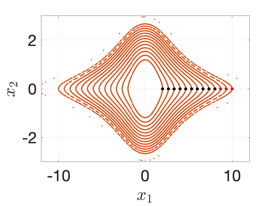
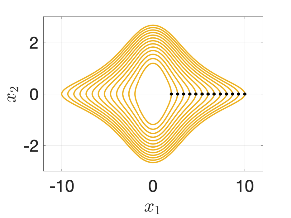
Numerical simulations using the MQAV midpoint method (MQAV-MP2) are presented in figure 2. As the ODE is Hamiltonian, there exist a number of methods with good structure-preserving properties for comparison. We will use the standard midpoint method (MP2) as well as AVF method. The midpoint method is symplectic and therefore has bounded Hamiltonian error. The AVF method preserves the Hamiltonian and is also a Runge-Kutta method known as Simpson’s method [12] corresponding to evaluation of the integral in (21) with Gaussian quadrature of order four. Furthermore, we remark that the MQAV-MP2 method with $\alpha=1/3$ also yields the AVF method. All methods are implemented using fixed point iterations with an absolute tolerance of $1.11\times 10^{-15}$. Using a time step of $h=1/10$ a total of 13 numerical orbits are plotted from the initial conditions $\bm{x}_{0}^{(i)}=(2+2i/3,0)^{T}$, where $i=0,...,12$, denoted by black dots. Red dots denote those initial conditions where the solution becomes unstable. We see that the midpoint method loses stability for the initial conditions corresponding to $i=8,...,12$, the AVF method loses stability for $i=10,...,12$ while the MQAV midpoint method retains stability for all initial conditions. We note that all three methods are unstable when $i=13$. Figure 2 also shows the Hamiltonian error as a function of simulation time. We see that the MQAV midpoint method and the Simpson method preserves the Hamiltonian up to machine precision for their stable orbits, whereas the standard midpoint rule does not. Lastly, we note that different choices of $\alpha$ affect the stability and accuracy of the method.

In this next example, we have designed an ODE with bounded orbits possessing two integrals, one of degree four and one of degree eight. The integrals are

References

- [1] Robert I McLachlan, GRW Quispel, and Nicolas Robidoux. Unified approach to Hamiltonian systems, Poisson systems, gradient systems, and systems with Lyapunov functions or first integrals. Physical Review Letters, 81(12):2399, 1998.
- [2] Ernst Hairer, Christian Lubich, and Gerhard Wanner. Geometric numerical integration: structure-preserving algorithms for ordinary differential equations, volume 31. Springer Science & Business Media, 2006.
- [3] Luigi Brugnano, Felice Iavernaro, and Donato Trigiante. Reprint of analysis of Hamiltonian boundary value methods (HBVMs): A class of energy-preserving Runge–Kutta methods for the numerical solution of polynomial Hamiltonian systems. Communications in Nonlinear Science and Numerical Simulation, 21(1-3):34–51, 2015.
- [4] Yuto Miyatake. An energy-preserving exponentially-fitted continuous stage Runge–Kutta method for Hamiltonian systems. BIT Numerical Mathematics, 54(3):777–799, 2014.
- [5] Hendrik Ranocha and David I Ketcheson. Relaxation Runge–Kutta methods for Hamiltonian problems. Journal of Scientific Computing, 84(1):1–27, 2020.
- [6] Arieh Iserles and Antonella Zanna. Preserving algebraic invariants with Runge–Kutta methods. Journal of computational and applied mathematics, 125(1-2):69–81, 2000.
- [7] Oscar Gonzalez. Time integration and discrete Hamiltonian systems. Journal of Nonlinear Science, 6(5):449–467, 1996.
- [8] Robert I McLachlan, G R W Quispel, and Nicolas Robidoux. Geometric integration using discrete gradients. Philosophical Transactions of the Royal Society of London. Series A: Mathematical, Physical and Engineering Sciences, 357(1754):1021–1045, 1999.
- [9] Toshiaki Itoh and Kanji Abe. Hamiltonian-conserving discrete canonical equations based on variational difference quotients. Journal of Computational Physics, 76(1):85–102, 1988.
- [10] GRW Quispel and David Ian McLaren. A new class of energy-preserving numerical integration methods. Journal of Physics A: Mathematical and Theoretical, 41(4):045206, 2008.
- [11] Ernst Hairer. Energy-preserving variant of collocation methods. Journal of Numerical Analysis, Industrial and Applied Mathematics, 5:73–84, 2010.
- [12] Elena Celledoni, Robert I McLachlan, David I McLaren, Brynjulf Owren, G R W Quispel, and William M Wright. Energy-preserving Runge-Kutta methods. ESAIM: Mathematical Modelling and Numerical Analysis, 43(4):645–649, 2009.
- [13] Takayasu Matsuo and Daisuke Furihata. Dissipative or conservative finite-difference schemes for complex-valued nonlinear partial differential equations. Journal of Computational Physics, 171(2):425–447, 2001.
- [14] Daisuke Furihata and Takayasu Matsuo. Discrete variational derivative method: a structure-preserving numerical method for partial differential equations. Chapman and Hall/CRC, 2019.
- [15] Elena Celledoni, Volker Grimm, Robert I McLachlan, DI McLaren, D O’Neale, Brynjulf Owren, and GRW Quispel. Preserving energy resp. dissipation in numerical PDEs using the “Average Vector Field” method. Journal of Computational Physics, 231(20):6770–6789, 2012.
- [16] Yuezheng Gong, Jiaxiang Cai, and Yushun Wang. Some new structure-preserving algorithms for general multi-symplectic formulations of Hamiltonian PDEs. Journal of Computational Physics, 279:80–102, 2014.
- [17] Yu-Wen Li and Xinyuan Wu. General local energy-preserving integrators for solving multi-symplectic Hamiltonian PDEs. Journal of Computational Physics, 301:141–166, 2015.
- [18] Morten Dahlby and Brynjulf Owren. A general framework for deriving integral preserving numerical methods for PDEs. SIAM Journal on Scientific Computing, 33(5):2318–2340, 2011.
- [19] Sølve Eidnes, Lu Li, and Shun Sato. Linearly implicit structure-preserving schemes for Hamiltonian systems. Journal of Computational and Applied Mathematics, page 112489, 2019.
- [20] Jie Shen, Jie Xu, and Jiang Yang. The scalar auxiliary variable (sav) approach for gradient flows. Journal of Computational Physics, 353:407–416, 2018.
- [21] Tomoya Kemmochi and Shun Sato. Scalar auxiliary variable approach for conservative/dissipative partial differential equations with unbounded energy. arXiv preprint arXiv:2105.04055, 2021.
- [22] Xiaofeng Yang, Jia Zhao, Qi Wang, and Jie Shen. Numerical approximations for a three-component Cahn–Hilliard phase-field model based on the invariant energy quadratization method. Mathematical Models and Methods in Applied Sciences, 27(11):1993–2030, 2017.
- [23] Yuezheng Gong, Yue Chen, Chuwu Wang, and Qi Hong. A new class of high-order energy-preserving schemes for the Korteweg-de Vries equation based on the quadratic auxiliary variable (QAV) approach. arXiv e-prints, pages arXiv–2108, 2021.
- [24] GJ Cooper. Stability of Runge-Kutta methods for trajectory problems. IMA journal of numerical analysis, 7(1):1–13, 1987.
- [25] Elena Celledoni, Brynjulf Owren, and Yajuan Sun. The minimal stage, energy preserving Runge–Kutta method for polynomial Hamiltonian systems is the averaged vector field method. Mathematics of Computation, 83(288):1689–1700, 2014.
- [26] G. R. W. Quispel Ari Stern Richard A. Norton, David I. McLaren and Antonella Zanna. Projection methods and discrete gradient methods for preserving first integrals of ODEs. Discrete and Continuous Dynamical Systems, 35(5):2079–2098, 2015.
- [27] GRW Quispel, HW Capel, et al. Solving ODE’s numerically while preserving all first integrals. Preprint, La Trobe University, Melbourne, 1997.
- [28] Robert I McLachlan. Spatial discretization of partial differential equations with integrals. IMA journal of numerical analysis, 23(4):645–664, 2003.
- [29] Robert I McLachlan. On the numerical integration of ordinary differential equations by symmetric composition methods. SIAM Journal on Scientific Computing, 16(1):151–168, 1995.
- [30] Zacharoula Kalogiratou, Theodore Monovasilis, and TE Simos. A sixth order symmetric and symplectic diagonally implicit Runge-Kutta method. In AIP Conference Proceedings, volume 1618, pages 833–838. American Institute of Physics, 2014.
- [31] M Suzuki and K Umeno. Higher-order decomposition theory of exponential operators and its applications to QMC and nonlinear dynamics. In Computer simulation studies in condensed-matter physics VI, pages 74–86. Springer, 1993.
- [32] Yuri B Suris. The problem of integrable discretization: Hamiltonian approach, volume 219. Birkhäuser, 2012.
- [33] Gengen Zhang and Chaolong Jiang. Arbitrary high-order structure-preserving methods for the quantum Zakharov system. arXiv preprint arXiv:2202.13052, 2022.
- [34] Benjamin K Tapley. On the preservation of second integrals by Runge-Kutta methods. arXiv preprint arXiv:2105.10929, 2021.