Two-level Systems Coupled to Graphene plasmons: A Lindblad equation approach
Abstract
In this paper we review the theory of open quantum systems and macroscopic quantum electrodynamics, providing a self-contained account of many aspects of these two theories. The former is presented in the context of a qubit coupled to a electromagnetic thermal bath, the latter is presented in the context of a quantization scheme for surface-plasmon polaritons (SPPs) in graphene based on Langevin noise currents. This includes a calculation of the dyadic Green’s function (in the electrostatic limit) for a Graphene sheet between two semi-infinite linear dieletric media, and its subsequent application to the construction of SPP creation and annihilation operators. We then bring the two fields together and discuss the entanglement of two qubits in the vicinity of a graphene sheet which supports SPPs. The two qubits communicate with each other via the emission and absorption of SPPs. We find that a Schödinger cat state involving the two qubits can be partially protected from decoherence by taking advantage of the dissipative dynamics in graphene. A comparison is also drawn between the dynamics at zero temperature, obtained via Schrodinger’s equation, and at finite temperature, obtained using the Lindblad equation.
I Introduction
The following paper is concerned with studying the entanglement of two two-level systems placed in close proximity to a graphene sheet. More specifically, we wish to study the communication of these emitters via so called surface plasmon polaritons (SPPs) that travel along the graphene sheet (see Fig. 1).

These SPPs are collective excitation of the electron gas that propagate along interfaces, and are usually produced in metal-dielectric interfaces with the aid of a prism, in setups such as the Kretschmann or Otto configurations. However, it is also possible to generate these excitations in a configuration where a graphene mono-layer is “sandwiched” between two dielectric media. This is because doped graphene acts as a conductor of electric charge, characterized by a sheet conductivity, which enables the existence of SPPs propagating on this material. (see Gonçalves and Peres 2016). In the configuration represented in Fig. 1, if two emitters are positioned close to the graphene sheet, they will interact with the surface plasmon bath and thus, emission and absorption of SPPs will provide a way of communication between them. This opens the possibility of creation of two (or more) entangled (in quantum mechanical sense) emitters. So, the aim and motivation for our work is two fold. We will on one hand describe the quantization of the SPPs for our configuration. We will do so via the dyadic Green’s function method, and this will shine light onto the propagation of these SPPs and how they will be used to establish a communication channel between the quantum emitters.
On the other hand, we will then focus on studying the dynamics of the emitters, that is, their time evolution. The final objective of our study is to show how dissipative currents in the graphene that correspond to the production of quantized SPPs will, in fact, protect the entanglement of the qubits and select a superposition of states over any other, extending its decay time (see Gonzalez-Tudela et al. 2011). To obtain the dynamics of the emitters, however, we must study their interaction with the plasmon bath. This can be modeled as a system interacting with a reservoir, and, to these kinds of problems, the theory of open quantum systems is particularly well suited. Indeed, at zero temperature, we can describe de dynamics of the emitters using the Schrödinger formalism. However, at finite temperatures, this formalism proves inadequate and the theory of open quantum systems has to be used.
The literature on application of the Lindblad equation to graphene is scarce to nonexistent, with a single paper, accordingly to a well known scientific data basis, focused on the interaction of two-level systems and graphene Nechepurenko et al. 2018 using the Lindblad equation.
The philosophy of writing of this paper was to keep the minimum of technical detail in the main part of the text. Thus, going through this part only, the reader will be able to capture the qualitative aspects of the problem. However, to master the details the reader has to work through the Appendices.
The paper is structured as follows: In section II we will first introduce the theory of open quantum systems with a focus on the Lindblad equation giving the main concepts toward its derivation. In section III a microscopic derivation of the Lindblad equation is given. We will use this theory to evaluate the dynamics of a quantum emitter coupled to a thermal radiation bath, which is one of the most studied applications of open quantum systems in quantum optics, and it will prove to be a good starting point for the study of the dynamics of similar systems. In section IV, we will quantize the SPP field using macroscopic Green’s functions methods, known as dyadic Green’s functions; we will consider the electrostatic limit, as a SPP is, for large wave vectors, insensitive to retardation effects. This will allow us to quantize the SPP field in the presence of dissipation and set the stage for the evaluation of the qubit dynamics. These are finally described in section V, where we study a single qubit coupled to the bath. The entanglement between two qubits mediated by SPPs as well as an investigation of the role of dissipation in this quantum mechanical process are performed in Sec. VI. All the details of the calculations are given in a set of Appendixes written using a didactic style.
II Steps towards the Lindblad equation
The aim of this section is to approach the theory of open quantum systems in general, providing a few significant steps toward the derivation of the master equation in Lindblad form without making reference to the particular properties of the system we wish to describe. Master equations describe the dynamical evolution of a quantum system which interacts with its environment (a so called open quantum system).
As stated, we will start without making reference to any particular system, following the approach of Manzano 2020, and will, a couple of sections ahead, specialize to actual applications of the theory.
Note that decoupling a system from its environment is a very significant endeavor both from a conceptual point of view, as well as from a practical perspective. On the conceptual side, a closed quantum system which does not interact with its environment, such as those treated in elementary quantum mechanics is merely a useful idealization as in nature nothing can be truly isolated. On the practical side, in some cases the environment of a system plays an important and useful role in its dynamics, and as such cannot be ignored. The goal of this section is therefore to introduce the necessary steps and approximations used in order to infer the evolution of the system of interest (which we will often call the reduced system) from those of the total “reduced system+environment" ensemble. The end result will be the so called Lindblad equation
| (1) |
This equation gives the time evolution of the density operator , which characterizes the state of the reduced system. The Lindblad equation can be interpreted as involving two contributions: A coherent evolution governed by the reduced system’s Hamiltonian corresponding to the commutator present in equation (1); and also an incoherent evolution brought on by the reduced system’s interaction with the environment. In this second term of the Lindblad equation there come into play a series of operators which are called jump operators that describe, for instance, the excitation and relaxation of the system’s state. The Lindblad equation is the most general trace-preserving dynamical equation with Markovian time-evolution (we shall clarify the meaning of these terms later).
To start with, we make a few comments on the formalism we shall use regarding composite systems. We may describe the reduced system by a wave-function that lives in a Hilbert space with an arbitrary complete basis . The environment can be characterized similarly by a Hilbert space with basis (we use the index for reservoir. In practice along the work we use the word reservoir or bath interchangeably with the word environment). The total system is characterized by the tensor product space with basis . The total Hamiltonian which characterizes the dynamics of the reduced system+environment ensemble can be constructed from the reduced system’s and environment’s Hamiltonians ( and respectively) as well as a coupling or interaction term as
| (2) |

As can be seen from the nature of the Lindblad equation (1), we will be using the density operator formalism and thus describe mixed states of the total system by a total density operator . corresponds to a tensor product of the reduced system density operator and the reservoir density operator (see appendix A for relevant definitions and calculations regarding the density operator and an application to the dynamics of an optically driven two-level system).
The density operator evolves according to the von-Neumann equation and its dynamics is governed by the Hamiltonian of equation (2). If we wish to describe the evolution of a system in contact with an environment in a quantitative and analytical manner we must proceed in lowest order perturbation theory.
Our goal is to make clear how the interaction of the system with its environment affects the dynamics and as such, we are really only interested in the time evolution brought on by the coupling . The reduced system itself can have non-trivial dynamics, so we want to separate the time evolution due to the coupling by writing the equations of motion in the interaction picture of quantum mechanics. In this representation, the density operator is and the coupling term in the Hamiltonian is . It is quite simple to show that the time evolution is given by the von-Neumann equation but with the total Hamiltonian replaced by the interaction term (see appendix A.2 for a discussion on the representations of quantum mechanics).
Another important tool which we shall employ often in the following considerations is the partial trace. It consists in a summation over a select number of degrees of freedom of the total system. For instance, one may take the partial trace over the reduced system degrees of freedom, or over the environment degrees of freedom. Tracing over the environment degrees of freedom, for instance, allows us to isolate the density operator for the reduced system from the total density operator. In symbols, we can write and thus, tracing over the reservoir we can write the von-Neumann equation for the system .
On the other hand, the von-Neumann equation for the total density operator lends itself to an iterative solution. Iterating once, and then tracing over the reservoir degrees of freedom, the following integro-differential equation for the time evolution of the system’s density operator is easily computed
| (3) |
The first term, containing is often neglected in the spirit of the molecular chaos hypothesis (see Hohenester 2020). It contains information regarding the initial state of the system, and we assume that initial correlations are meaningless in the evolution of the system. In practice, this term can actually be shown to be 0 in many cases such as if the environment is thermal.
We also neglect the system-reservoir interaction to first order. This is the so called Born approximation, which allows us to write . This approximation imposes that we work in the weak coupling regime, and, as such, the evolution of the system occurs over a much larger time scale than the correlation and relaxation time scales of the system and , i.e. we have . We may assume that we start from an uncorrelated state , for example by considering that the system and environment have not interacted before . After this initial point in time, we assume that the system and reservoir stay uncorrelated, or that correlations are sufficiently small to be ignored. This is a very strong assumption which is the first of three key approximations we use to derive the Lindblad equation, and is a necessary step to unravel the system from its environment.
We also make the approximation which allows us to obtain a time-local equation. This approximation is called the first Markov approximation since now the system can be described by at the single time in a manner which does not depend on its past history. This kind of evolution is called Markovian. This constitutes the second key approximation in our journey toward the Lindblad equation. If we assume the case of a thermal environment and reservoir is in thermal equilibrium, or more generally that the environment has many more degrees of freedom than the system and thus the interaction changes the environment in a negligible manner, loses its time dependence and the time-evolution of the density operator is given by
| (4) |
where we have considered for simplicity that . We have proceeded in a quite general manner and the previous equation has many of the characteristics we want, but we still need further work in order to transform equation (4) to a form that we can actually compute any physical quantity. In many cases the interaction Hamiltonian can be written as a tensor product of operators
| (5) |
where as indicated by the indices acts on the Hilbert space of the system and on the Hilbert space of the reservoir . We can now perform a series of simple expansions and calculations to write the master equation in a more suitable form. Firstly, we substitute the interaction Hamiltonian of the form (5) into the master equation and evaluate the commutators explicitly. Then, factoring the expression, and cyclically permuting the operators and allows us to introduce several additional simplifications (see appendix B for details regarding these and following calculations). Finally, we can introduce the correlation functions
| (6) |
where the super-index in the operators has been omitted for simplicity. The idea is that, given a concrete physical system, we can approach the derivation by calculating these correlation functions by hand first and then replacing them in the master equation to obtain the time evolution. Note that the first Markov approximation ceases to be an approximation and becomes exact only when these correlation functions are proportional to . Such proportionality would indeed allow us to replace by . The third, and final, key approximation we introduce is to assume that the integrand decays fast enough with time, thus letting us extend the integral to infinity. To do this we perform the change of variables and let the upper limit of integration go to infinity. This procedure is the second Markov approximation and it results in the Redfield equation written in terms of correlation functions, which will allow us to give a derivation of the Lindblad equation in physical applications. The Redfield equation reads
| (7) |
For instance, we shall derive the Lindblad equation in the case of a two-level system (qubit) coupled to the thermal E-M field in a later section. We note that the procedure we are going over in this section is often described as a microscopic derivation of the Lindblad equation, since we explicitly construct the Lindblad jump operators from the Hamiltonian, however there are many ways to derive this equation, and in principle one could also derive it from macroscopic principles, such as positivity of the density operator as well as linearity of the time–evolution, along with the Markov approximations.
III Microscopic derivation of the optical master equation in Lindblad form
III.1 Thermal radiation - A short review
Before we concern ourselves with continuing the derivation of the Lindblad equation, it is useful to first discuss the concept and some of the mechanics of thermal radiation. In particular we aim to discuss thermal radiation field states and derive the state distribution and average photon number when a mode of the E-M field is in thermal equilibrium with its environment at some temperature . These kinds of states are incoherent superpositions of Fock states. From thermodynamics, it is well known that the probability of a field mode being in the th excited state, or in other words, that there are photons occupying a certain mode is given by a Boltzmann factor
| (8) |
where is Boltzmann’s constant and is the partition function of the E-M field. Using this we may calculate, for instance, the average number of photons in such a thermal field state, in a single mode characterized by a frequency . This amounts to summing the occupation numbers for each state, weighted by the probability . With the previous Boltzmann factor and using the formula for the energy of the harmonic oscillator (note that rigorously the energy is written , however, since the partition function would then be written , we can cancel this factor), this can be evaluated as a derivative of the geometric series which yields the famous result
| (9) |
This is the Bose-Einstein distribution for photons. Thus depends on the interplay between the mode energy and the inverse thermal energy . Notice, of course, that we can arrive at this same result using a more quantum mechanical approach involving the density operator formalism. The density operator is where is the Fock state with photons. The distribution of states is the expectation value of the number operator, which we can calculate by tracing over the degrees of freedom of the field. This procedure equivalently yields the Bose-Einstein distribution.
Another relevant quantity beyond the distribution of these thermal states, is the density of states, or mode density, of the field, which corresponds to the number of allowed modes with wave-vector between and . To evaluate it, we need only count the number of allowed modes inside a sphere of radius in -space. If we let the E-M field be quantized over a volume then the wave vector can only have certain values (see appendix C). We thus integrate over the sphere in -space and divide by the effective volume occupied by each mode, which is . The resulting integration kernel is the mode density
| (10) |
where is the speed of light.
III.2 Derivation of the Lindblad equation for a two-level system coupled to thermal radiation
We now proceed with the derivation of the Lindblad equation by using our previous considerations regarding thermal radiation to compute the master equation for a two-level system coupled to the E-M field when in thermal equilibrium at a temperature . We follow the approach outlined in Carmichael and de Bruxelles 1993; Carmichael 2013. By the end of this section, we will be able to write the master equation in Lindblad form. Our starting point is the master equation for a system coupled to a reservoir. We have derived this in section II to lowest order perturbation theory, where upon introducing the Born and first Markov approximations we were left with a Markovian dynamical equation that gave the time evolution for the system. By assuming that the interaction Hamiltonian could be written as a sum of tensor products of operators which act on the space and reservoir separately, we were able to write the master equation in terms of reservoir correlation functions and thus we now actually apply this equation to a two-level system interacting with thermal radiation.
To proceed, we need the Hamiltonians for the reduced system (two-level atom), the reservoir (E-M field in thermal equilibrium at temperature ), as well as the coupling Hamiltonian (responsible for the light-matter interaction). The treatment of the two-level system is simple enough (see appendix D) as the Hamiltonian can be described in terms of a Pauli matrix
| (11) |
The two-level system is coupled to the E-M field, which has the Hamiltonian
| (12) |
where and are the creation and annihilation operators for photons. Note that we have chosen to neglect the term that usually comes with the Hamiltonian, since we are only interested in the evolution caused by energy differences measured with respect to the vacuum state. The coupling Hamiltonian is yet to be determined. It is well known that in the dipole approximation the light-matter interaction Hamiltonian has the form of a scalar product of the electric field with the dipole moment, but this is a semi-classical description which does not take into account the quantization of the E-M field. To arrive at the full description of this operator we substitute the electric field for the electric field operator in the Hesinberg picture, derived in the appendix C.
For a single mode, the Hamiltonian is time independent and given in terms of the number operator by . The time evolution in the Heisenberg Picture of the creation and annihilation operators ( and ) is quite simple. In fact, we give a brief derivation, in appendix C, which shows they oscillate in time with frequencies and respectively. This makes it so we can construct the electric and magnetic field operators from these operators in the Schrodinger picture quite readily, from which the interaction Hamiltonian follows. The Hamiltonian has, in principle, a complex structure, involving all combinations of the two-level system raising and lowering operators (, where and are the second and third Pauli matrices respectively) with creation and annihilation operators for photons and ), but we can simplify the dynamics by converting to the interaction picture, performing the rotating wave approximation (RWA) and then converting back to the Schrodinger picture (see appendix B). In terms of the two-level system raising and lowering operators , we can write the interaction Hamiltonian in the Schrodinger representation as
| (13) |
where the summation of the previous equation occurs over both the wave-vectors as well as the polarization components . We have also introduced the coupling constants
| (14) |
to group together the prefactors coming from our manipulations. Specifically, in performing the several calculations, this coupling constant depends on the inner product between the polarization vector and the dipole moment of the two-level system and on the permittivity of free space .
In the rotating wave approximation, the interaction Hamiltonian describes photon absorption and emission by the two-state atom which leads to its excitation and de-excitation respectively. We can now compare the form of the interaction Hamiltonian to the master equation we had written in terms of reservoir correlation functions. In the interaction picture we can make the identifications
| (15) |
thus, in the master equation we sum over and . The reservoir correlation functions are, in this case, given by
| (16) |
where we have used the orthogonality of the states to arrive at the results in the first line. We have also employed the Bose-Einstein distribution for photons at temperature as well as the relation to obtain the expectation values of the number operator needed for the results of the second line. Making use of the density of states , we replace the sum over the modes in the reservoir correlation functions with an integral over the mode density. Then, we can introduce the previously discussed first and second Markov approximations, through which we write and let go to infinity. In this regime we are able to use the Sokhotski-Plemelj theorem (see appendix E) and explicitly write the master equation as
| (17) |
where H.c. stands for the Hermitian conjugate and we have introduced the coefficients
| (18) |
where denotes the Cauchy principal value of the integrals. We wish now to introduce a more symmetric grouping of these terms, such that the underlying physics becomes more apparent. Firstly we write out all the terms of equation (17) making the Hermitian conjugate explicit and then grouping together common factors in , , and . We also make use the of the Pauli matrix identity . Converting back to the Schrodinger picture we then obtain
| (19) |
where . Note in particular that this equation is easily written in Lindblad form
| (20) |
where, the sum occurs over and we have introduced the jump operators and . In this form, we have made clear the existence of the Lamb shift in the frequency corresponding to Hamiltonian of the two-level system. The operators , jump from the ground to excited state and vice-versa with decay rate and excitation rate .
Note, in particular, that there are two contributions to the emission rate. The first is temperature independent and given by , while the second is temperature dependent and given by . The former corresponds to a spontaneous decay rate and the latter to stimulated transitions induced by thermal photons. The same goes for the Lamb shift, since the term is temperature independent and corresponds to the normal Lamb shift and the term gives the ac Stark shift associated with the thermal radiation field. As for the excitation rate, there exists a single term given by .
We also note that these calculations give a correct prediction for the Einstein A coefficient ( in our notation), associated with the spontaneous emission of light. With the density of states given by equation (10) and the coupling constants of equation (14) and making a suitable choice of coordinates in -space it is simple enough to evaluate as given in equation (18). We obtain
| (21) |
and thus, we see that our open quantum systems approach gives the correct result for the Einstein A coefficient and as such, a correct prediction for the spontaneous decay rate for the two-level system. This shows an agreement of the Wigner-Weisskopf theory prediction of the Lamb shift and Einstein A coefficient (see Hecht 2000) and the open quantum systems approach. The latter also predicts an ac Stark shift which is not taken into account by the former method. This extension of the quantum mechanical description to a finite temperature regime is something we will explore in more detail in the following sections.
IV Quantization of the surface plasmon polariton field via the dyadic Green’s function method
IV.1 An introduction to dyadic Green’s functions
In this paper, our final aim is to study the interaction of qubits and the exchange of information via surface plasmon polaritons (SPPs) in a graphene sheet. We thus now step away from the theory of open quantum systems and step foot into the realm of macroscopic quantum electrodynamics (macroscopic QED), which can be characterized as the study of the quantized E-M field in the presence of macroscopic media (see Scheel and Buhmann 2009, Buhmann 2013). The aim of this section is to introduce an important tool of macroscopic QED, called the dyadic Green’s function or Green’s tensor. This is quite a remarkable object because it allows for the characterization of absorption and dispersion properties in media characterized by a certain electric permittivity and a certain magnetic permeability . This is especially noteworthy since the description it provides is non-classical, despite the emergence of the Green’s tensor from Maxwell’s equations, which are a phenomenological and classical description of macroscopic systems. In general, the Green’s tensor as a mathematical object plays the role of the usual Green’s function for partial differential equations in the case of vector equations. In particular, we will use it to find a solution of the inhomogeneous Helmholtz equation for the electric field
| (22) |
where again is the electric field at a given point in space and frequency , is the electrical current at that point, is the magnetic permeability of free space and is the relative magnetic permeability of the medium.
As stated, the idea of the mathematical application of the Green’s tensor is much the same as that of the usual Green’s function (see Paknys 2016 for a thorough introduction to dyadic Green’s functions), in the sense that we want to turn a partial differential equation problem, into a linear algebra problem. The Green’s tensor will play the role of the inverse to the differential operator in question. We can state the general second order ordinary differential equation problem, up to transformations of the variable , as
| (23) |
with and . The aim of the Green’s function method is to present a solution in terms of an integral. To do so, we find a function for which
| (24) |
This function is the namesake Green’s function (see appendix F.1). There are usually several methods at our disposal for finding such functions. We go over two of them in full generality in the appendixes, F.2 and F.3, the first of which makes use of the Dirac- function and the second of eigenfunction expansions. Simply put, and as already stated, the general idea is to proceed as in linear algebra, where if we want to solve a matrix equation we simply try to find the inverse operator , which is possible as long as 0 is not an eigenvalue of . The same approach is valid for the dyadic Green’s function , which is constructed from a solution of the Helmholtz equation with a Dirac-delta source
| (25) |
where is the identity dyadic. Much like in linear algebra an operator is the inverse of an operator if . In the case of the Helmholtz equation, a solution for the electric field can thus be constructed from as an integral
| (26) |
Physically, the Green’s tensor contains the geometry and physical properties of the involved media, and will play a role in the microscopic description of dissipation, as we shall later see. We will be able to think of it as an electric response function that will carry the interaction generated by the current from the point to the point .
We present in the appendix F.4 a derivation for the Green’s tensor in free space for which we make use of the Dirac- method, while in the following section we will derive this quantity for the case of SPPs in graphene via the eigenfunction expansion method, which will prove to be a more challenging endeavor.
IV.2 Deriving the Green’s tensor for our system
A surface plasmon polariton (SPP) is a two-dimensional electromagnetic excitation that lives in dielectric-metal interfaces, or in more complicated geometries such as the one we are considering, where a graphene sheet is embedded or “sandwiched” between two semi-infinite dielectrics. This configuration can be described by a dielectric function over the whole space of the form (see Gonçalves and Peres 2016 for discussions regarding the conductivity of graphene).
| (27) |
where is the conductivity of the graphene sheet. For the dielectric function is a constant while for the dielectric function is also constant and equal to . This information is contained in the Heaviside theta functions written in equation (27). At we have a contribution from the graphene sheet. This dielectric function defines the system we are interested in studying because it contains, as a macroscopic quantity, all the microscopic information about the media that make up the system.
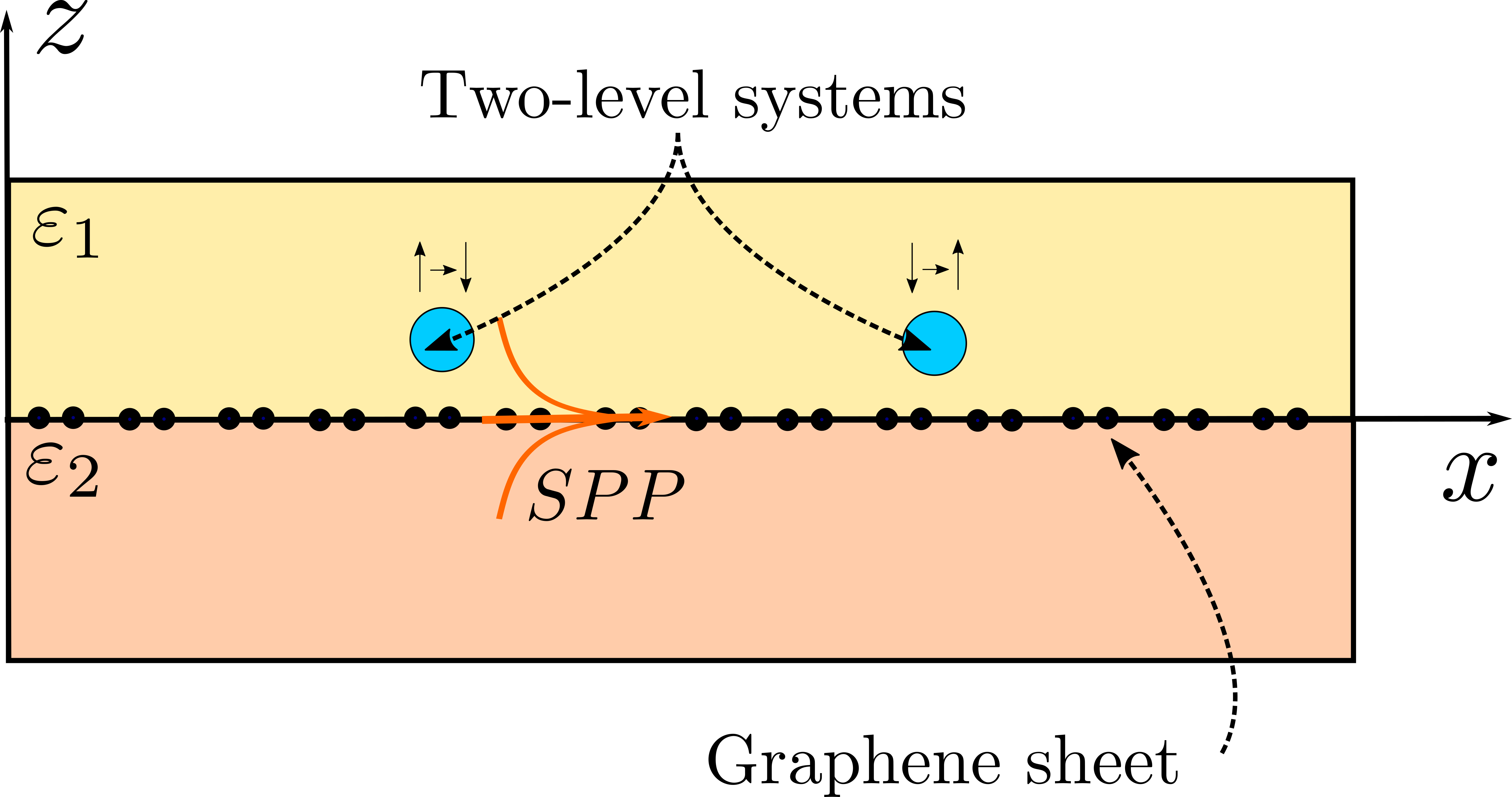
Our discussion will now focus on essentially two topics. The first is actually finding the Green’s tensor for SPPs traveling along the Graphene sheet, and the second is then using this Green’s tensor to follow through with a quantization scheme for the SPPs based on the presence of Langevin noise currents in the Graphene (see Matloob et al. 1995).
To find the Green’s tensor we work in the Weyl or temporal gauge (see Loffelholz et al. 2003; Haller 1987; Creutz 1979) we have the scalar potential . In this gauge, the vector potential and the electric field are related through and the magnetic field can also be derived from . The electric field relation allows for the Helmholtz equation to be written in terms of the vector potential. Assuming that no currents exist within the dielectric media on both sides of the graphene sheet, we obtain
| (28) |
Our approach will make use of an expansion in eigenmodes, from which the Green’s function will be calculated (see Søndergaard and Tromborg 2001) as
| (29) |
where the integral is over corresponding to the plasmon wave-vector, are the eigenvalues, a normalization factor, and the eigenmodes, which are solutions to the equation
| (30) |
Note that and all depend on but we omit this dependence for the sake of lightening up the notation. Equation (29) can be written as an eigenvalue problem , with the operator . This is still a complicated equation, but writing it in this form makes it somewhat easier to handle. In fact, we already know all the pieces to the puzzle, since all that we are looking for are solutions in the form of SPPs. These correspond to evanescent waves along the axis, with a small penetration depth along the dielectric media (in fact this penetration depth can be remarkably small and thus graphene plasmon polaritons are much more confined than usual SPPs, see Luo et al. 2013; Principi et al. 2018), and to traveling waves along the graphene sheet. This suitable choice of solution conceptually closes the problem, since all we have to do is substitute the form of the SPP eigenmodes
| (31) |
where the index shows that these propagate in the medium with while the index shows that these propagate in the medium with , into equation (30). We then write this as a matrix equation, solve for the eigenvalues and normalization and then substitute this all into equation (29) to find the Green’s function. Of course things are not so easy in practice since this procedure is mathematically challenging, but also, several noteworthy physical insights can be derived by performing it. We leave most mathematical details to the appendix F.5 and focus on the physical aspects of the derivation. The first of these insights may be brought to the limelight when noticing that in indexing the eigenmodes with the medium they propagate in, we are actually “splitting” our solution in two, and thus we will have two sets of eigenvalues and which for each should actually correspond to the same SPP mode, and therefore should agree with each other. This imposes a constraint which allows us to connect the solution across the graphene sheet as well as relate with and through the relation
| (32) |
The second insight one gains comes from the form of the eigenvalues themselves. In fact, upon examining the eigenvalues present in the appendix F.6 we notice that they are degenerate for , which means they must indeed be superpositions of and polarization vectors and with (see Sipe 1987). Since SPPs have only polarized modes, then we shall only retain this polarization with eigenvalue . To further connect the solution for and we look at the boundary condition for the electric field at . In particular, we have . Noting the relation between the electric field and vector potential that stems from the Weyl gauge, we can use it to relate the amplitudes of the modes in both media, labeled and . The boundary condition yields the relation . We can also use the boundary condition for the magnetic field and Ohm’s law in the graphene sheet to provide some additional constraints into the wave-vector and allow us to relate it to the frequency . All this procedure results in a dispersion relation
| (33) |
which, when assuming a conductivity computed with the Drude model, and if we perform the electrostatic approximation , gives the final dispersion relation for SPPs which we will use throughout the rest of this manuscript
| (34) |
where is the Fermi energy, is the fine structure constant and is the mean dielectric constant. The normalization constant can also be found quite readily as described in the appendix F.7. The calculation yields, in the electrostatic approximation, . Now, we have only to put these pieces together and crank the mathematical engine (and by cranking the mathematical engine we mean calculating 16 integrals of Bessel functions over the complex plane, the details of which are presented in the appendix F.8, F.9, and F.10). Making use of equation (29) to construct the SPP part of the Green’s tensor. After toiling over the calculations, one finds the dyadic Green’s function
| (35) |
where is a function of frequency such that the dispersion relation reads , and is the angle that the vector corresponding to the position at where the Green’s function is evaluated, makes with the axis. Finally the matrix has diagonal elements
| (36) |
and off-diagonal elements
| (37) |
We now conclude this section where we have found the SPP part of Green’s tensor for the specific geometry of a Graphene sheet embedded between two dielectrics. We shall later see that it is this Green’s tensor, or rather, its imaginary part that plays a role in the interaction between matter and the SPPs, determining specifically the decay rates for two level systems.
IV.3 Quantization of surface plasmon polaritons using dyadic Green’s functions
In this section we take a step back from the specific form of our Green’s tensor and analyze a quantization scheme for SPPs utilizing the method of dyadic Green’s functions. Our approach will be based on the introduction of Langevin-noise currents in graphene to model dissipation. This procedure is outlined in Allameh et al. 2015 in the case of a general dissipative medium. Here is the longitudinal spatial coordinate, and is the frequency of the noise current. These dissipative noise currents will then be the basis upon which we construct the bosonic creation and annihilation operators for the SPPs. To solve for the electric field with these currents present, we will have to solve an non-homogeneous Helmholtz equation of the form
| (38) |
to which, as we know from the previously discussed mathematics of Green’s tensors, a solution can be provided in the form of an integral
| (39) |
In the Weyl gauge, since the Lagrangian density of the E-M field is , we can find the canonically conjugate variable to by calculating . This means that when we promote the vector potential and the electric field to operators, we have the canonical commutation relation . This result holds in general, but since we are interested only in the commutation relations for the SPP part of the fields, we instead impose the commutation relation , where we have replaced the full Dirac-delta function with a longitudinal delta function (see the appendix G.1 for a brief note regarding transverse and longitudinal delta functions).
In addition to this, we impose that the Langevin-noise currents satisfy the commutation relations where and are a constant and a function determined so that equation (39) is consistent with both commutation relations for the operators , as well as . We go over the derivation of and in detail in the appendix G.2, but the derivation is quite simple as we need only to substitute equation (39) into the commutator, bring the Green’s tensors outside it and then substitute the commutation relation for the noise currents in. A few tricks are then necessary (see appendix H for the details), but one can show that with the propper choice of and , it is possible to write the commutation relations for our system consistently and therefore “normalize” the commutation relation for the noise currents into a bosonic commutation relation which yields the SPP creation and annihilation operators
| (40) |
This result allows us to write the vector potential operator and the electric field operator in terms of these -operators, and therefore this concludes the section on the quantization of the SPP field, as we can now write
| (41) |
where the electric field operator in the Schrodinger picture was obtained by taking the Fourier transform of at . We see that the quantized field is connected deeply with the Green’s tensor, and in fact this macroscopic quantity appears directly when the field is written in terms of the creation and annihilation operators for the SPPs.
V Time evolution of a single qubit coupled to a plasmonic bath in thermal equilibrium
In this section we bring together the two thematically disconnected parts of this study we have so far discussed, and make use of the theory of open quantum systems and dyadic Green’s functions, with which we arrived at the SPP field creation and destruction operators and respectively, to describe the dynamics of a two-level system coupled to a plasmonic bath. The theory of open quantum systems will come into play, since the SPP field will (at a finite temperature ) act as a thermal reservoir of SPPs which will constitute an environment to which the two-level system is coupled. Therefore, much like in the case of the thermal E-M field, we proceed with a microscopic derivation of the master equation in Lindblad form. We start with the study of the dynamics of a single qubit coupled to a plasmonic bath in thermal equilibrium.
To develop our theory we need the Hamiltonians for the single qubit, the reservoir (SPP field in thermal equilibrium at temperature ), and the coupling Hamiltonian. We set the ground state of the two-level system with zero energy, which amounts to the choice of a reduced system Hamiltonian of the form
| (42) |
instead of the usual . The Hamiltonian of the SPP field is constructed from the vector potential operator and reads
| (43) |
The interaction Hamiltonian can also be constructed from these operators in the Schrodinger picture. It contains mixed terms involving the creation and destruction SPP field operators, as well as the raising and lowering operators for the qubit. The dyadic Green’s function will then carry the interaction from , which is the position of the qubit to , where the SPP is created. The summarized procedure leads to written in the Schrödinger picture
| (44) |
where, we have defined . Although these Hamiltonians appear to be significantly more complicated than that of simple thermal radiation, the procedure is essentially the same as before, since we can separate the coupling Hamiltonian into a tensor product of operators and
| (45) |
The aim is to calculate the reservoir correlation functions, which in this case correspond to thermal averages of equation (6) but with the and as defined in equation (45). This is no easy task and in fact conceals several mathematical subtleties, because in order to calculate the correlation functions it is necessary to evaluate the thermal averages of the -operators. In the literature (see Philbin 2011), it is often simply assumed that the following relations hold, due to the mathematical subtlety of the evaluation of the thermal averages
| (46) |
We include in the appendix I, however, a derivation based on discretizing the integrals in frequency and position that come up in the Hamiltonian. We notice still, that the reservoir correlation functions present in equation (6) are written in the interaction picture, however, a simple derivation included in the appendix H shows that their representation in this picture is entirely analogous to the representation of usual creation and annihilation operators. After substituting the reservoir correlation functions back into the Redfield equation and performing both the Born and Markov approximations, we obtain a master equation of entirely the same form as equation (19) which we repeat here for convenience
| (47) |
with . Here, however, the decay rate as well as the normal Lamb shift and thermal shift due to the SPP field are dependent on the imaginary part of the Green’s tensor which is obtained via an integral of a product of Green’s tensors (see appendix F.11). Their form can be written as
| (48) |
where the kernel is defined as
| (49) |
The previous equation can also be brought into Lindblad form by defining the jump operators
| (50) |
Note that we can explicitly evaluate the imaginary part of the Green’s function for our system, which yields a decay rate
| (51) |
where and are the transverse and longitudinal parts of the two-level system dipole moment , is the SPP wave-vector, and is the SPP wavelength. This result is seen to match others found in the literature, for instance those by Ferreira et al. 2020; Koppens et al. 2011. of course corresponds to the spontaneous decay rate from the excited to the ground state of the qubit coupled to the SPP field. In fact, expanding the density matrix in the Lindblad equation and solving for each probability we obtain the coupled rate equations
| (52) |
Note in particular that when the temperature becomes very small, in the sense that , then the Bose distribution function vanishes and we are left with the dynamics
| (53) |
which can also be obtained via Shcrodinger’s equation (see appendix J.1). Thus, we see clearly that the coupling between the SPP field and the qubit is described via the Lindblad equation in a manner which is consistent with the zero temperature description characteristic of the Schrodinger equation, where initially the qubit is excited and there is no SPP present in the graphene because there is no thermal excitation of the plasmon gas. The open quantum systems approach, however, allows for a finite temperature description as well. The effect of temperature is visible if we make some plots as in Fig. 4.


VI Time evolution of two qubits coupled to a plasmonic bath in thermal equilibrium
We can now extend the previous discussion to the case we really want to study, in particular the case of two qubits close to the graphene sheet (the case of two color centers near a transition metal dichalcogenide single layer has been studied already by Henriques et al. 2021). What we find, when we evaluate the coherent part of the dynamics (equivalently the Schrodinger dynamics of the system with a zero temperature SPP field) is that, as expected, the system will oscillate between the states denoted and , where each qubit is excited, however there will also be an overall decay due to the losses in the graphene sheet. This oscillation is caused by the introduction of a coupling rate between the qubits and an additional energy shift coming from their interaction. We shall later provide their definition explicitly. A physical description of this phenomenon may be obtained when we note that the Green’s tensor will not only propagate the interaction from the position of each qubit to itself when written , but also propagate the interaction from one qubit to the other when written , giving rise to the additional rates and shifts.
We find that the oscillations occur at a rate that depends on and the total populations decay slower as . When , the probability of finding the state in the states and oscillate around . Due to the dissipation, the amplitude of these oscillations will diminish in time, and both states will eventually tend to an equilibrium situation with equal probability . Details regarding the derivation of the dynamics can be found in the appendix J.1. We can see the dynamics of the qubits in Fig. 5a.
An alternative and perhaps clearer picture can be obtained when we repeat this analysis for the “Schrodinger cat” states and . We see that the for close enough to , the state decays very quickly, while the state is protected from decoherence via the dissipative dynamics. In fact for the state is stationary with probability and the only interchange that occurs is between the states and . We can plot the probability of finding the superposition states explicitly as in Fig. 5b. The moral we can extract from this discussion is that dissipative dynamics in graphene allow us to isolate one Schrodinger cat state over the other.
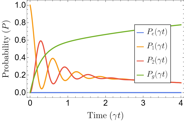
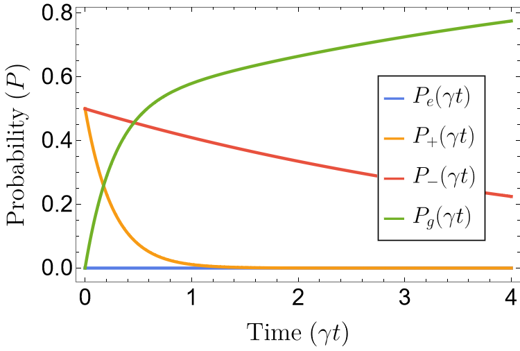
The dynamics at zero temperature are summarized in Fig. 6 (see also Gonzalez-Tudela et al. 2011). The state will decay quickly with rate , while the state will be protected from decoherence as it decays much slower with rate . The state where both qubits are excited and where both are in the ground state have more straightforward dynamics as their populations either decay or increase with overall rates going to/coming from the states .

An extension of this discussion can be performed in the case of finite temperature by making use of Lindblad dynamics. A derivation of the Lindblad equation for a two qubit system coupled to the plasmon field proceeds in a manner which is very similar to the case of a single qubit, with a few notable distinctions. We go over this derivation in detail in the appendix J.2 but it suffices to say that because the summation of the jump operators now occurs not only over the states of a single qubit, but rather of both of them, there come into play terms which describe the emission of a plasmon by one of the qubits followed by absorption by the other. These terms lead to additional shifts in energy which must be included in the coherent evolution of the system, as well as additional rates that set a time-scale for the communication between the qubits. These rates are given by the same expression as for the spontaneous decay rate for a single qubit coupled to the plasmon bath, but with the dyadic Green’s function evaluated at each position of the two qubits thus leading to a kernel
| (54) |
where is the average dielectric constant of the mediums between which the graphene sheet is immersed, and is the Green’s tensor evaluated at the position of both qubits. This kernel leads, by means of similar definitions to those of equation (48), to the rates and shifts
or explicitly for the additional decay rate
| (55) |
Notice that we can interpret this in a somewhat physical manner by noting that the Green’s tensor is propagating the interaction between them. The Lindblad equation can thus be written as
| (56) |
where the jump operators match those defined for the single qubit except for the index running over the two qubits and . The jump operators also match these but give the interaction between the qubits and so are constructed in a similar manner but with the rate instead of . In the case of finite temperature, working in the basis has some additional value, since the Lindblad equation becomes self-contained within the diagonal elements. In other words, one would in principle have to calculate the solution for a coupled set of 16 differential equations to evaluate the dynamics (one corresponding to each element of the density matrix). Hermiticiy of the density matrix brings this number down to 10, but in this basis, the diagonal elements, which correspond to the populations depend via the Lindblad equation only on each other (see appendix J.2), and therefore we only have only to solve a set of 4 coupled differential equations to obtain the population dynamics.
A simple numerical evaluation of the Lindblad equation yields Fig. 7.


Once again, from Fig. 7, we see that the zero temperature dynamics predicted by the approach based on the Schrodinger equation are reproduced by the Lindblad equation (compare Fig. 5 with Fig. 7a), which is really astonishing considering the differences in formalism. As temperature increases some of the coherence is lost for longer times, as all states, including the ground state tend to equilibrium at probability .
VII Conclusions and outlook
In the present study we aimed to investigate a physical system where two two-level systems (qubits) interact via emission and absorption of surface plasmon-polaritons (SPPs) in a graphene sheet placed between two semi-infinite dielectrics. The evaluation of the Green’s tensor from the macroscopic Maxwell’s equations allowed us to quantize the SPP field and somewhat remarkably derive a quantized description of the SPP field with dissipation, by arriving at creation and annihilation operators of the SPPs. We studied in detail the derivation of the master equation in Lindblad form using the Born and Markov approximations for a single qubit coupled to a thermal electromagnetic field, and used this as a stepping stone for the following analysis. This consisted in studying the dynamics of one and two qubits coupled to the SPP reservoir, via the Schrodinger equation as well as the Lindblad equation. From a practical perspective, the results obtained using the Lindblad equation matched those of the Schrodinger equation when we considered the temperature to be absolute zero. Otherwise, the Lindblad equation allowed the extension of these results to a finite temperature regime, where the SPP reservoir plays an active role in the qubit dynamics.
These calculations revealed some interesting behavior in the qubit dynamics as the dissipation introduces an asymmetry between the time evolution of what we called “Schrodinger cat states” corresponding to superpositions of the states where one qubit is excited while the other is in the ground state. Effectively, this asymmetry manifests in a larger decay rate for one Schrodinger cat state over the other. This in turns leads to a protection from decoherence, where entanglement is maintained and a superposition is isolated over a longer time-frame than would otherwise be possible. We find this quite a beautiful result, where we are able to take advantage of dissipation in macroscopic media to maintain coherence in a quantum mechanical system. Not only is this an interesting result in itself, but we can envision a continuation of this work, where the usage of graphene-based metamaterials allows for the consideration of an anisotropic conductivity and thus the manipulation of SPP using wave-guides (see Bilow 2003; Gomez-Diaz et al. 2015a; Gomez-Diaz et al. 2015b)
Acknowledgments
∗TVCA performed all the calculations and produced the first written version of the paper.
†NMRP conceived the idea, supervised the work, and contributed to the writing in the final stage of the work.
N.M.R.P. acknowledges support from the European Commission through the project “Graphene-Driven Revolutions in ICT and Beyond” (Ref. No. 881603, CORE 3) and COMPETE 2020, PORTUGAL 2020, FEDER and the Portuguese Foundation for Science and Technology (FCT) through project POCI-01- 0145-FEDER-028114. The Portuguese Foundation for Science and Technology (FCT) is acknowledged in the framework of the Strategic Funding UIDB/04650/2020. Both authors acknowledge Dr. Bruno Amorim for providing the derivation found in Appendix J. N.M.R.P. Dr. Bruno Amorim and João Carlos Henriques for discussions on the Lindblad equation.
Appendix A The density operator
A.1 General definitions
In this appendix we follow Hohenester 2020 for a brief description of the density matrix formalism. We start by considering a quantum system to be in a state and an hermitian operator to be acting on the system’s Hilbert space, we define its expectation value as
| (57) |
This observable provides information as to the outcome of an experiment where we have absolute certainty that the system is in the state . We might however find some kind of statistical uncertainty in the systems state before measurement. That is to say that to know that the exact state of the system is often difficult to know in practice since we have only imperfect information. To make this observation quantitative we may think about an ensemble of almost identical systems, where the state is not , possibly due to the system’s interaction with its environment. Rather, we may find that the system exists in a superposition of states with probability distribution . In this case, the expectation value is given by the weighted sum
| (58) |
We note the difference between the statistical uncertainty in the system’s state and the quantum mechanical uncertainty which is accounted for by the quantum mechanical expectation value. To account for these different uncertainties and corresponding averages we develop a formalism based on the density operator. This is the mathematical tool that describes our knowledge of the system. If we consider a complete basis of the system’s Hilbert space made up by the states , then the trace of an operator is defined by
| (59) |
This is in analogy to the trace of a matrix as the sum of its diagonal elements. The cyclic property of the trace reads
| (60) |
By decomposing the states in the complete basis of the Hilbert space with states , we can write the expectation value in as
| (61) |
Note that the states may not form a complete basis. As such, for convenience we introduce a definition for a density operator
| (62) |
Following these considerations we introduce the concept of a pure state as a unit vector in the Hilbert space of a certain system. This is opposed to the concept of a mixed state, which is represented by a positive unit trace operator corresponding to the density operator. Using this operator, the expectation value can be succinctly written as
| (63) |
This definition for expectation value is thus more general as it accounts for two kinds of averaging
- •
The quantum mechanical averaging over the eigenvalues of a given hermitian operator when acting on a pure state.
- •
The statistical averaging over the probability distribution of the state of the system itself .
We now note some of the properties of the density operator as defined above. Its trace is
| (64) |
where we have used both the fact that and . Note also that for a pure state , that is a state in which there exists no statistical uncertainty, we may compute the density operator as
| (65) |
which is easily seen to obey the projector relation
| (66) |
In essence, this imposes an upper limit on the trace of . Since, in general
| (67) |
The trace is, thus
| (68) |
By the Cauchy-Schwartz inequality, we get
| (69) |
where the equality in the second step holds only if for all and , which can only happen if the state is pure and equation (66) is satisfied. Thus we can identify a valid density operator by two abstract properties
- •
- •
These properties do indeed have important physical meaning. The fact that the trace of the density operator is unity represents the normalization of mixed states. A system must be in some state after all, and as such, the total probability of finding it in any state should add up to one. On the other hand, the trace of the square of the density operator measures the purity (and indeed this quantity often bares that name) of the state. If it is a pure state then . On the other hand, for a mixed state, . In fact the purity is bounded by where is the Hilbert space dimension. The lower bound is obtained for the maximally mixed state, where all populations are (see Jaeger 2006). A practical note on the density operator may be that of course, in a finite dimensional Hilbert space it can be represented by a matrix in an arbitrary basis . In this basis we have or
| (70) |
The diagonal elements of this matrix are often called the populations, whereas the off-diagonal elements are called the coherences.
A.2 Pictures of quantum mechanics
In this appendix we give a brief overview of the pictures of quantum mechanics. For a thorough overview see Jishi 2013.
A.2.1 Schrodinger Representation
Unitary transformations play an important role in quantum mechanics, and in fact, the time evolution operator is unitary. This operator takes a wave-function at time and propagates it to time .
| (71) |
If we insert this expression into the Schrodinger equation, we may write an operator equality
| (72) |
which can also be written in integral form as
| (73) |
We can now look at time evolution from different perspectives, and as such come up with several different pictures or representations of quantum mechanics. Firstly, in the Schrodinger picture, the wave-functions are time dependent, and their evolution is given by
| (74) |
As time evolves, only the wave-functions change and the operators stay unchanged.
A.2.2 Heisenberg Representation
In contrast, in the Heisenberg picture, the wave-functions are time independent, and only the operators evolve in time, according to
| (75) |
Note that the observable corresponding to the expectation value in both pictures is the same. We may prove this succinctly
| (76) |
We may calculate the time evolution of an operator in the Heisenberg picture taking the derivative of an operator in the Heisenberg picture
| (77) |
By making use of the integral equation (73) we can simplify the previous equation by calculating
| (78) |
which by the fundamental theorem of calculus gives
| (79) |
We then get, by substituting into equation (77)
| (80) |
By making use of the definition of the time evolution of an operator in the Heisenberg picture, we write
| (81) |
which can be written in a form known as the Heisenberg equation of motion
| (82) |
As time evolves, only the operators change and the wave-functions stay unchanged.
A.2.3 Interaction or Dirac Representation
There exists still another picture called the interaction or Dirac picture. This is useful when considering perturbed Hamiltonians of the form
| (83) |
where is treated as a perturbation. We introduce a time evolution operator , which is associated only with the evolution governed by the Hamiltonian . In this picture, both the wave-functions and operators evolve in time according to
| (84) |
We can prove, yet again that this picture produces the same results for the expectation value
| (85) |
We can still define the evolution operator of the interaction picture as
| (86) |
Taking its time derivative, and invoking once again the fundamental theorem of calculus when using equation (73), write
| (87) |
where the perturbation in the interaction representation is defined as . As such, in the interaction picture, the time evolution operator in the interaction picture is given by the solution of the equation
| (88) |
By noting that this last equation can be written in integral form as
| (89) |
The time evolution operator depends only on this perturbation, and as such the dynamics of the system can be computed by making use only of since the zeroth order Hamiltonian has been completely absorbed into the computation of and therefore into the time evolution operator and wave function in the interaction picture. The integral of equation (89) can be solved iteratively
| (90) |
and thus, to first order in the perturbation , we have
| (91) |
As such, the time evolution of an operator in the interaction picture is calculated from differentiating from the general expression (89) with respect to on both sides. This gives
| (92) |
or simplifying the expression using the commutator
| (93) |
and the time evolution of a wave-function is
| (94) |
As time evolves, both the wave-functions and operators change. This is an intermediate representation between the Schrodinger and Dirac pictures.
A.3 Time evolution of the density operator
We note that we can write the time evolution of a given state ket as well as the corresponding bra by making use of the time dependent Schrodinger equation with a time dependent Hamiltonian
| (95) |
As such, we can construct the time evolution of the density operator by using its definition as stated in equation (62). Thus, computing the derivative of the density operator, we get
| (96) |
By pulling the Hamiltonian out of the sum and simplifying the notation by recognizing the density operator, we may still write
| (97) |
We have thus arrived at the von-Neumann Equation for the Time Evolution of
| (98) |
This equation can be solved in the interaction picture, by making use of the time evolution operator of equation (86). The time evolution is thus governed by
| (99) |
where corresponds to the density operator at time . Unitary time evolution is, as discussed, one of the postulates of quantum mechanics. It is in fact, a very natural postulate, which is realized in the conservation of the norm of states and means that normalized states stay normalized.
A.4 Time evolution of the Bloch vector in a two-level system
In this section we analyze a two-level system (see appendix D) form the density operator perspective and give the time evolution of the Bloch vector. The density operator of a two-level system is written as
| (100) |
where is the identity, is an arbitrary Bloch vector and is the vector containing the Pauli Matrices. We note immediately that:
| (101) |
This implies that
| (102) |
and we also note that
| (103) |
where taking the trace, we get
| (104) |
Noting that in a two level system the Bloch vector has norm such that 1, then the operator of equation (100) verifies the second condition of a density operator, and thus, since it also verifies the first by virtue of the result in equation (102), it is indeed a valid density operator. The expectation value of can thus be calculated utilizing
| (105) |
which corresponds to a way of calculating the elements of the Bloch vector. We can now aim to calculate the time evolution of a Bloch vector in a two-level system. By employing the result of equation (105) we can write
| (106) |
and by now making use of the von-Neumann time evolution, we write
| (107) |
By cyclically permuting the operators under the trace, which is allowed by equation (60), we finally write
| (108) |
This result based on the density operator formalism reproduces the well known result for the evolution of the components of the Bloch vector in a two-level system but is in fact more general since it also applies to mixed states, where the additional statistical averaging is needed.
A.5 An application of the density matrix formalism in the interaction picture - Optically driven two-level system
We have so far described two-level systems in terms of the evolution of the components of the Bloch vector, but we might as well pick a basis made up by a ground state and an excited state , which we do following Lavine 2018. In this basis our time dependent wave-function in the Schrodinger picture can be written as
| (109) |
Of course and are in principle complex and as such amount to four time-dependent functions. Of course, if this is to be consistent with the Bloch formalism, we know there must be a constraint, which is simply the normalization condition
| (110) |
To explicitly find the matrix elements of the density operator in this basis, we just need to calculate
| (111) |
| (112) |
| (113) |
| (114) |
which along with the von-Neumann equation for the time evolution of the density matrix allows us to calculate explicitly the time evolution of the density operator for a given Hamiltonian. We aim now, however, to solve this in the case of a perturbed system, for example in the case of a time dependent harmonic electric field. We first approach this problem using the von-Neumann equation in the Schrodinger picture but later we shall see that the usage of the interaction picture may provide much simpler results. We star with the general form of a perturbed Hamiltonian
| (115) |
where in the basis we have
| (116) |
and the matrix elements of our perturbed Hamiltonian are therefore
| (117) |
The time evolution of the density matrix elements is given in the Schrodinger representation by the von-Neumann equation (98)
| (118) |
and noting that only the terms that obey the conditions imposed by the Kronecker-delta survive, we write
| (119) |
or more succinctly, in terms of the commutator
| (120) |
which corresponds to the von-Neumann equation in the Schrodinger representation for two-level systems. We now proceed to convert this result to the interaction picture, which will simplify our calculations. Specifically the interaction picture removes the time dependence due to To start, we write the interaction picture wave-function as
| (121) |
We follow this up by calculating in the interaction picture. This is simply
| (122) |
The density operator in the interaction picture can be constructed from the wave-functions. It is given by
| (123) |
and noting that the von-Neumann equation in the Schrodinger representation for a perturbed Hamiltonian is
| (124) |
if we make use of equation (123) and multiply on the right by and on the left by on both sides, we can write as well as differentiate both sides with respect to time and multiply by , we have
| (125) |
Comparing with the von-Neumann equation in the Schrodinger picture, and noting that the Hamiltonian commutes with its own exponential, we have that
| (126) |
and, multiplying on both sides by before solving for
| (127) |
This result is the von-Neumann equation in the interaction picture. We shall now use this to calculate the time evolution of an optically driven two-level system. The first step is to specify the form of the perturbation or interaction Hamiltonian. We consider this to be that of a time dependent electric field in the dipole approximation
| (128) |
and in particular, we will consider a harmonic field, oscillating with a positive and negative frequency. That is to say
We now calculate, as in the general case, the matrix elements of this perturbation
| (129) |
Since is odd, then for the bra-ket vanishes. As for the remaining matrix elements, we calculate them in the interaction picture using . Since for the eigenstates of the zeroth order Hamiltonian, the evolution is trivial, then
| (130) |
and similarly for
| (131) |
The density operator has thus only non-diagonal elements. To simplify our notation we introduce the Rabi energies defined through
| (132) |
and a frequency . For simplicity, if we write , we have a perturbation of the form
| (133) |
With the intent of using the von-Neumann equation in the interaction picture we calculate the commutator
| (134) |
and we note that this equality is equivalent to a system of equations
| (135) |
We now apply the rotating wave approximation and keep only the resonant terms containing or . We are left with
| (136) |
If we introduce the parameter and and admit that the system is originally in the ground state, which corresponds to and it is possible to solve this system of equations. This solution is difficult to obtain, however we can simplify the calculations assuming that the system is in resonance and . This removes the time dependence and we obtain a much simpler system of equations of the form
| (137) |
If we take the time derivative of the first equation, we obtain the second order differential equation
| (138) |
and we now employ the equations for the time derivatives of the relevant matrix elements in equation (137). We obtain
| (139) |
and remembering that the trace of the density matrix is 1, we write
| (140) |
We propose a solution of the form and see if it solves the differential equation
| (141) |
Indeed, canceling all the terms proportional to sines and cosines, we get that the equality holds if . We also make use of the initial conditions
| (142) |
which mean that the two-level system is initially in the ground state. Using these, we can find
| (143) |
and as such, we have a solution for the matrix element in resonance, which reads
| (144) |
As for we need not calculate its evolution in the same manner. We can simply invoke that the trace of the density matrix should be one. This leads us to
| (145) |
As for the non-diagonal elements of the density matrix, we can now substitute these last few results into equation (137) and obtain
| (146) |
which can easily be solved to yield
| (147) |
Finally, noting that we have the full solution to the time evolution of the density operator
| (148) |
This example serves as a somewhat pedagogical introduction to calculations of the time evolution of the density matrix, which is useful when more complex cases arise ahead.
Appendix B Details of the derivation of the Lindblad equation
B.1 Considerations regarding the general derivation of the Lindblad equation
In this appendix we provide a few discussions and steps which were skipped over or just mentioned in the main text along the general considerations made toward the Lindblad equation as well as its derivation in the case of the two-level system in contact with the thermal reservoir.
We make a few remarks regarding the procedure of simplification of the made in the main text more explicit. Starting from the integro-differential equation for the von-Neumann equation it was stated that the commutators were explicitly calculated for a interaction Hamiltonian of the form given in equation (5). Indeed the result of this procedure is:
| (149) |
Dropping the tensor products and and indices for the operators which make up the interaction as well as the index, and then factoring the expression, we are able to write:
| (150) |
Under the trace over the reservoir degrees of freedom we can cyclically permute the operators and . Doing this allows us to further simplify the previous equation:
| (151) |
and finally, introducing the correlation functions, we write:
| (152) |
This is the equation (7) presented in the main text except for the use of the first and second Markov approximations.
B.2 Detailed derivation of the light-matter interaction Hamiltonian in the rotating wave approximation
Here we provide a detailed derivation of the light-matter coupling Hamiltonian in the rotating wave approximation. We start with the semi-classical light-matter Hamiltonian.
| (153) |
To arrive at the full description of this operator we want to substitute the electric field for the electric field operator . Note that this operator depends on time since the quantization of the E-M field was done in the Heisenberg representation. We must therefore convert to the Schrodinger picture. In the Heisenberg Picture we have
| (154) |
For a single mode, the Hamiltonian is time independent
| (155) |
and therefore, the time evolution of the ladder operators in the Heisenberg Picture is given by
| (156) |
where we have used in the next to last step the commutator property . Thus, by taking the complex conjugate, we also obtain the equation of motion for the creation operator
| (157) |
They therefore have solutions of the form
| (158) |
We can identify these in the operator for the electric field and make the inverse correspondence in order to obtain the operator in the Schrodinger picture
| (159) |
and thus, the interaction Hamiltonian is
| (160) |
We write the operators in the interaction picture, using
| (161) |
Since the harmonic oscillator Hamiltonian does nothing to the Pauli matrices, then
| (162) |
and using the fact that , where , we have and therefore
| (163) |
In a similar manner, the raising and lowering operators in the interaction picture as
| (164) |
Following the same procedure and using the previously calculated commutator, we have
| (165) |
and therefore, if we switch to the interaction picture and write the interaction Hamiltonian, we have
| (166) |
The simplification we introduce is the rotating wave approximation in which we discard terms in high frequency and retain only those that can resonate. Thus we have
| (167) |
which when converting back to the Schrodinger picture, becomes
| (168) |
We see that the rotating wave-approximation retains only the terms which correspond to simple photon absorption and emission. We may further simplify notation by introducing the coupling constants defined as
| (169) |
such that the interaction Hamiltonian for a single mode is written as
| (170) |
Thus, the full Hamiltonian describing the light-matter interaction is a sum over the modes
| (171) |
which is the desired form for the light-matter Hamiltonian in the Schrodinger picture and rotating wave approximation.
B.3 Writing the Lindblad equation in terms of correlation functions and their calculation
In this section we give more detail on the identifications made to write the master equation of the two-level system coupled to the thermal radiation field. In the Schrodinger picture, comparing the light-matter Hamiltonian with the general form given in equation (5), we write
| (172) |
with which the Hamiltonian is written
| (173) |
Of course, these operators can be converted to the interaction picture using the previously derived identities for and the ladder operators of the E-M field is given as in the equation (165). As such, the sum of equation (173) is over and , and we can evaluate the reservoir correlation functions as
| (174) |
and a similar calculation yields
| (175) |
Finally, the cross terms evaluate to
| (176) |
and since , we have
| (177) |
where we have used in the last step that the density operator has unity trace. In these considerations we have also used the mean photon number we had previously derived for the E-M field in thermal equilibrium at temperature . Using these correlation functions we can write the master equation as
| (178) |
We have seen that two of these terms vanish since the reservoir correlation functions evaluate to 0. Additionally, for simplicity we take . Thus, the master equation reduces to
| (179) |
We can also introduce the change of variables . Thus, we write
| (180) |
where again, H.c. stands for the Hermitian conjugate and finally we make use of the density of states of equation (10) to evaluate the reservoir correlation functions. We replace the sum over the modes with an integral over the mode density
| (181) | ||||
| (182) |
We conclude this section of the appendix remarking that with the reservoir correlation calculated, we may now substitute them into the Redfield equation. This next section is devoted to finishing the calculation and writing the master equation in Lindblad form.
B.4 Markov approximations and writing the master equation in Lindblad form
If we introduce the Markov approximation, through which we write the only dependence on comes from the correlation functions. We also let go to infinity (second Markov Approximation), regime in which we are able to evaluate via the Sokhotski-Plemelj identity of appendix E
| (183) |
where is the Cauchy principal value. Thus we introduce the definitions
| (184) |
As such, we have
| (185) | ||||
| (186) |
These simplifications allow us to write the master equation as
| (187) |
but, as stated in the main text, we wish now to introduce a more symmetric grouping of these terms, such that the underlying physics becomes more apparent. Firstly we write out all the terms of equation (187) making the Hermitian conjugate explicit
| (188) |
We then group together common factors
| (189) |
Making use of the identities of equation (245), we write the previous equation as
| (190) |
which further reduces it to
| (191) |
The final step in the derivation of the master equation is to convert back to the Schrodinger picture. We can use the following relation
| (192) |
and invert it to write
| (193) |
From here, we can use the substitute the master equation and obtain
| (194) |
We rearrange the previous expression using the commutator relations of and to bring the exponentials to either side of the density operator in the interaction picture. The contributions from the commutators arising from rearranging the operator products cancel each other out and thus, we are left with
| (195) |
where . We note that we can define
| (196) |
With these operators, we have
| (197) |
and with some further rewriting, we are able to bring the master equation into the Lindblad form presented in the main text.
B.5 Calculation of the Einstein A coefficient
To provide a check on the open quantum systems approach, we calculate the coefficient which in fact corresponds to the Einstein A coefficient as it gives the rate for spontaneous emission of photons. It was originally defined as
| (198) |
The density of states in a single direction is given in equation (10) and the coupling constants in equation (169). We thus have to solve
| (199) |
where we have considered the atom to be located at the origin and thus . To evaluate the angular integral we chose the first polarization component to be such that . The second polarization component will make an angle with . Thus
| (200) |
if we choose such that it is aligned with we have
| (201) |
and thus
| (202) |
which can be easily shown to yield
| (203) |
which is the correct result for the Einstein A coefficient and gives the spontaneous decay rate for the two-level system.
Appendix C Quantization of the electromagnetic field in free space
In this appendix we quantize the E-M field in free space in a macroscopic manner. We follow the most common approach, which can for instance be found in Milonni 2019. Our starting point for this section is the Maxwell’s equations in the absence of currents and charges. These read
| (204) |
These can be rewritten in terms of the scalar potential and vector potential . In particular, if we work in the coulomb gauge, we have that . In this gauge the vector potential contains all the information about the magnetic and electric fields, since
| (205) |
Calculating the time evolution for the vector potential therefore allows us to obtain the time evolution of the E-M fields. This is done with the use of Ampère-Maxwell law, which reads
| (206) |
If we substitute here the fields by the vector potential it is easy to arrive at
| (207) |
which we can simplify a lot using the identity. Since we are working in the Coulomb gauge the first term will be and therefore we are left with
| (208) |
This is just a wave equation for the vector potential. Therefore the dynamics of the E-M field in a vacuum can be obtained by solving a wave equation for the vector potential. The solutions of the equation may for instance be simply plane waves of the form
| (209) |
where in this equation is the polarization vector, a complex amplitude, is the wave-vector, is the polarization state and the frequency associated with the wave. If we assume that we are solving the wave equation over the whole space then is unrestricted and can have any value. If however, for simplicity we confine the field in a finite volume or impose periodic boundary conditions, then will only be able to have certain values. If we consider for instance a box of side such that then in the left and right as well as top and bottom and front and back of the box the phase factors must coincide. This of course implies that only discrete wave vectors are allowed, namely those such that
| (210) |
These discrete wave-vectors together with their polarizations constitute the allowed modes of the field. In terms of these modes we can express a general field through Fourier decomposition. This amounts to summing over the modes and their complex conjugates such that the electromagnetic vector potential is real
| (211) |
If we want to derive the electric field from this vector potential we simply do as in equation (205) and take the time derivative. We arrive at
| (212) |
Similarly if we take the curl of we might write the magnetic field as
| (213) |
Since we have the expression for the E-M fields, we may now calculate the energy stored in the volume . Classically, this is simply the integral over the energy density
| (214) |
where we have used the suggestive notation for the energy. Note that this can be simplified to
| (215) |
We first calculate the magnetic contribution to the energy
| (216) | ||||
where noting that
| (217) |
the whole expression simplifies and using that we have
| (218) |
Doing the exact same calculation for the electric contribution, we have
| (219) |
and thus, the total energy is
| (220) |
Which corresponds to a sum of the energy over the several modes of the system. Note that we did not commute and add together the complex numbers precisely because this brings out a fortuitous comparison that we can make with the energy levels of a harmonic oscillator. This gives us a hint toward the following considerations we can make for the quantization of the E-M fields. The fundamental idea is that to each mode of the radiation field, we associate a harmonic oscillator. The degree of excitation of this harmonic oscillator gives us the number of photons that occupy a mode. Thus, the term photon acquires a precise definition in this context. A photon is an excitation of the harmonic oscillator associated with a mode of the E-M fields. The Hamiltonian for a harmonic oscillator is
| (221) |
If we associate one such Hamiltonian to a mode, then the total Hamiltonian will of course be the sum over the modes of each individual Hamiltonian
| (222) |
Note the striking similarity with the equation (220) for the classical energy stored in the E-M field in the volume . We can in fact make a simple correspondence between equations (222) and (220) by introducing the quantization rules
| (223) |
For notation’s sake we compress both indices and into a single . Thus, for each mode, the creation operator acts by creating a photon in this mode, while the destruction operator acts by removing a photon from the mode
| (224) | ||||
| (225) |
Also, it is possible to measure how many photons occupy each mode by acting with the number operator since
| (226) |
These states with a precisely defined photon number are called Fock states but we may also consider states which are superpositions of these states an thus do not have a defined number of photons.
Since we have determined the quantization rules which give us the creation and annihilation operators for the radiation field, we may now construct the operator which corresponds to the vector potential
| (227) |
From this operator we may also construct the field operators that correspond to the electric and magnetic field by using equations (205). We have for a single mode
| (228) |
Of course, the total operators are given by a sum over the modes
| (229) |
and note also, that quite generally, these field operators can be decomposed into parts which oscillate with positive and negative frequencies as
| (230) |
Using the quantization rules, one has that the photon Hamiltonian is given by
| (231) |
which acts on a general Fock state with many modes (multi-mode Fock state) as
| (232) |
In general we shall, in the main text and following appendices work with thermal states, which are indeed multi-mode Fock states with a probability distribution given by the canonical distribution.
Appendix D Two-level systems
In this appendix we go over a few useful properties of a two-level system (two-state atom or qubit), with states characterized by energies and respectively. The energy corresponds to the excited state while corresponds to the ground-state. Of course the states are labeled such that . We will make use of the Pauli matrices as in particular, the system Hamiltonian for a two-level system is of course
| (233) |
which can be written in a more convenient form as
| (234) |
where the Pauli matrix corresponds to
| (235) |
Choosing the energy reference so that the zero is in the middle of the energies and In this case the Hamiltonian is just
| (236) |
which we can write as
| (237) |
We may want to describe the light-matter interaction for this two-level system. To do so we need to write the dipole operator conveniently, and as such, if we introduce the frequency , we note that it can be expanded in terms of a complete basis of the system’s Hilbert space
| (238) |
In the case of the two-level system this reduces to
| (239) |
and thus can define the dipole operators
| (240) |
With this notation we write
| (241) |
It may be also worth noting that the expectation value of the dipole operator has a particular simple realization in the density operator formalism. It is given by
| (242) | ||||
Of use in our considerations are also the identities
| (243) |
| (244) |
| (245) |
These will be used throughout the text very often, for instance the last equation (245) represents in the case of a two-level system, a freedom in the choice of the zero of the energy. If we choose the zero to be exactly in the middle between the excited and ground states, the Hamiltonian will read , where is the energy gap between excited and ground state. If we make the zero of the energy coincide with the ground state, then we can write . Both these representations for two-level atoms are used throughout the paper, and equation (245) is useful as a transition between them.
Appendix E The Sokhotski-Plemelj identity
This appendix is dedicated to obtaining a result that is used again and again throughout the paper. It is sometimes referred to as the Sokhotski-Plemelj theorem or identity, and states that
| (246) |
For completeness, we prove this identity here, noting again that we will often employ it. We start by performing a change of variables and write
| (247) |
This integral can be regularized by adding a small imaginary part to the frequency , and solving the integral before letting it go to 0.
| (248) |
where is written so as to omit the limit. This form of writing the integral is often utilized, but note that it is merely a formal expression. It is in fact a distribution, and makes sense only inside an integral. We can manipulate it as
| (249) |
We now can calculate the following quantity
| (250) |
For the first integral we find, when it approaches and when , approaches . Additionally, since
this is a nascent function, which means
| (251) |
For the second integral, when , that when , we have
| (252) |
but when , we have
| (253) |
where the last line of equation (253) follows from the fact that . As such, we have
| (254) |
and by putting the results together we have proved the Sokhotski-Plemelj theorem, that states
| (255) |
Thus, we conclude this section, introducing the notation
| (256) |
and noting that we shall often call upon this result.
Appendix F Details on the calculation of the Green’s function
F.1 The idea behind Green’s functions
We start this appendix with a few considerations and a refresher on the Green’s function method for ODEs following the approach of Kirkwood 2011. We discuss how to solve a non homogeneous linear second-order ordinary differential equation with given boundary conditions by presenting the solution in terms of an integral. More precisely we find a function for which
| (257) |
with and and
| (258) |
This function is the namesake Green’s function. We shall obtaining via two usual methods. The first will make use of the Dirac-delta function and the second of eigenfunction expansions.The general idea is to proceed as in linear algebra, where if we want to solve a matrix equation
| (259) |
we simply try to find the inverse operator , which is possible as long as 0 is not an eigenvalue of . We shall also see that if is not an eigenvalue of , we shall also be able to construct the Green’s function that provides the unique solution to , with appropriate boundary conditions.
F.2 Construction of Green’s function using the Dirac-delta function
We provide first some intuitive motivation for this approach. If we let
| (260) |
We are trying to solve
| (261) |
for such that . Suppose there is a function for which
| (262) |
we can multiply both sides by and integrate with respect to . Doing so, we have
| (263) |
If we can pull the operator outside the integral, we have
| (264) |
and thus
| (265) |
is a solution to the equation
| (266) |
Note that the previous considerations are sound, however we need a way to construct the Green’s function. We first find such that it satisfies the homogeneous equation for .
The solution will have two parts, one for and . If we suppose that these solutions are and respectively. Then the Green’s function can be written as
| (267) |
We then need to find each and the Green’s function becomes fully determined. To do this we use the boundary conditions
| (268) |
along with continuity at . This means that
| (269) |
Additionally, the derivative of the Green’s function can be shown to have a discontinuity at :
| (270) |
The final condition is that it is symmetric and thus
| (271) |
From these boundary conditions one can obtain the coefficients and thus determine the Green’s function.
F.3 Construction of Green’s function from eigenfunctions
We continue to consider the operator
and want to solve the equation
with boundary conditions
Suppose that is a complete orthonormal basis for the vector space consisting of eigenvectors of that satisfy the boundary conditions and that is the eigenvalue of . If we equip the vector space with the inner product
We then have
where
| (272) |
and therefore we want to find the ’s to construct the solution. Since is a linear operator and is an eigenvector of with eigenvalue for each we have that
We get a relation for the coefficients since and therefore
| (273) |
and since is a basis, we can equate the previous equation term by term
| (274) |
Since is not an eigenvalue, we can write
| (275) |
and thus
| (276) |
If we recall that , we have
| (277) | ||||
which, if we can exchange the summation and integral due to proper convergence properties of the functions, we can write as
| (278) |
Thus, the Green’s function is
| (279) |
The crucial step to construct the Green’s function using this method is thus to find the eigenvalues and eigenfunctions for that satisfy the initial conditions. Note that an alternative is to consider the problem
| (280) |
where is not an eigenvalue of and thus, one obtains the Green’s function
| (281) |
One can easily show, however that one form can be converted into another by suitable renaming of and .
F.4 Dyadic Green’s functions using the Dirac- - Example of a single dipole
In this appendix we introduce the dyadic Green’s function as a natural extension of the Green’s function discussed in the previous section for the case of a vector equation. We focus on a critical and instructive example of the wave equation for the electric field
| (282) |
We introduce the wave number . The Green’s tensor, or dyadic Green’s function is defined through
| (283) |
where is the unit matrix. Similarly to the procedure followed in the previous section, we can multiply on both sides by and integrate over the whole space.
| (284) |
and thus this is a particular solution to the non-homogeneous equation. If is a solution to the homogeneous equation, the general solution is of the form
| (285) |
To find the Green’s function we assume that the source of current is a dipole at , which means that . The integral of the previous equation is thus immediate, and reads
| (286) |
In the Lorentz gauge, we can write the electric and magnetic fields in terms of a scalar and vector potential and . In this gauge we have
| (287) |
If we substitute the electric field in the electric field equation, we have
| (288) | ||||
or
| (289) | ||||
and using the fact that we have
| (290) | ||||
where finally canceling the electric field term, we have
| (291) |
and if we replace the current with that produced by the dipole we have
| (292) |
We get a differential equation for the components of the Green’s function associated with the vector potential
| (293) |
This equation can be solved using the Fourier transform. If we define
| (294) |
the differential equation (293) reduces to
| (295) |
We can then make an inverse Fourier transform arriving at
| (296) |
We can perform the integral by contour integration noting that there is a pole at . We have
The result allows us to write
| (297) |
Factoring the above expression we have
| (298) |
which allows us to identify the dyadic Green’s function in real space as
| (299) |
where is a dyadic differential operator and is the tensor product. This serves as an example of the computation of a dyadic Green’s function using from a Dirac- function.
F.5 Finding the eigenmodes
In this appendix we begin the quantization of surface plasmons via dyadic Green’s functions. Contrary to the previous section we shall not use the construction from a delta function, but rather an expansion of eigenfunctions (eigenmodes in this case).
The problem we are interested in solving consists of a graphene sheet embedded between two semi-infinite dielectrics. As such, for the dielectric function is a constant while for the dielectric function is also constant and equal to . At we have a contribution from the graphene and therefore the dielectric function over the whole space can be written as
| (300) |
where is the conductivity of the graphene sheet. In the Weyl gauge (see Loffelholz et al. 2003; Haller 1987; Creutz 1979) we have that , where is the electric field and is the vector potential. We thus have a wave equation reading
| (301) |
where we have assumed that there are no currents in the dielectric. The graphene sheet is a boundary condition for this wave equation. We will solve this equation via a dyadic Green’s function. It is such that
| (302) |
and our first goal is to construct this dyadic Green’s function. Our approach will make use of an expansion in eigenmodes. We write the Green’s function as
| (303) |
where are the eigenvalues, a normalization factor, and the eigenmodes, solutions to the equation
| (304) |
which we can write as
| (305) |
Since the system has dissipation is not hermitian and the left and right eigenmodes are not the same. The left eigenmodes are
| (306) |
or
| (307) |
The normalization factor can be found by evaluating
| (308) |
We assume and want to solve for mode functions of the form
| (309) |
where the index shows that these propagate in the medium with while the index shows that these propagate in the medium with . This is the desired form for our problem since we are interested in solutions to the equation that propagate like waves along the graphene sheet and decay exponentially as we go along into the dielectric media corresponding to the surface plasmon polariton solutions. Substituting this form into equation (304) one can easily check that it can be written as a matrix equation
| (310) |
for . We can solve this system for the eigenmodes and corresponding eigenvalues. These are
| (311) |
The eigenvalues for the dielectric on the other side of the graphene sheet is obtained by replacing and . We have, for this case
| (312) |
An important observation, however, is that each eigenvalue with the same index on both sides of the graphene sheet must correspond a single mode across the whole system. In symbols, this must mean that . This allows us to connect the solution across the graphene sheet and relate with and . We can do this by equating
| (313) |
Note however that the eigenvalues are degenerated for . They must indeed be superpositions of the and polarization vectors
| (314) |
where . We can find the and polarization components for by writing as a function by using equation (313). Note that if we substitute these polarizations into the matrix equation (310) for the eigenmodes, we have
| (315) |
and similarly for the with the previously mentioned substitutions. The same eigenvalue solves the equation for the polarization. In particular, we want to solve only for plasmonic eigenmodes, which only have polarization.
F.6 Boundary conditions - Dispersion relation in the electrostatic limit
We now proceed with connecting the solution for with that for . We have the usual boundary conditions for Maxwell’s equations. For the electric field we have
| (316) |
which we can translate into an equation for the eigenmodes since . Using then the polarization, which is parallel to the graphene sheet at , we have
| (317) | ||||
from where follows
| (318) |
The boundary condition for the magnetic field will take into account the surface current that propagates along the graphene sheet. We can write it as
| (319) |
where we have used Ohm’s law. The magnetic field can be evaluated as . Explicitly, we have
| (320) |
and thus making the usual substitutions we find . Thus
| (321) |
We have the additional constraints from the boundary condition
| (322) | ||||
which yields
| (323) |
or rewriting
| (324) |
and recalling the equation (313) that related , and , we can write
| (325) |
and solving for , we have
| (326) |
and therefore
| (327) |
The conductivity can be computed using the Drude model, with which we have
| (328) |
where is the Fermi energy and is the momentum relaxation rate. This corresponds to an approximation of the form The dispersion relation can be written as
| (329) |
and replacing with the result of equation (326) in this equation we have
| (330) |
or in other words
| (331) |
or yet
| (332) |
This allows us to write the eigenvalues as
| (333) |
and in the electrostatic approximation
| (334) |
where and where we have introduced the surface plasmon polariton (SPP) frequency as
| (335) |
The first form is valid for a Drude conductivity and the second in general. The dispersion can therefore be found when or in other words
| (336) |
or rather still
| (337) |
which also means that
| (338) |
This is an implicit equation for the spectrum of the SPPs, which may be solved analytically or numerically depending on the complexity of .
F.7 Finding the normalization constant
In the previous appendix we have found the eigenmodes and eigenvalues, as well as written them in a convenient form, relating , and through the boundary conditions of our problem. To find the Green’s function, in this appendix find the normalization coefficient . For the polarized modes we can evaluate the normalization as
| (339) |
where the first term covers , the second and the final comes from the graphene boundary condition at . We have, choosing
| (340) |
which if we use that we can write more simply as
| (341) |
In the electrostatic limit, we have and thus we can write for the case when
| (342) |
We can further write this result using the dispersion relation of equation (338), and this way obtain
| (343) |
F.8 Construction of the dyadic Green’s function
In the present appendix we note that the dyadic Green’s function can then be computed taking only into account the mode with polarization. It reads
| (344) |
In the limit the polarization vectors can be written as
| (345) |
where and thus, evaluating the tensor product explicitly, and then substituting the forms of and , we have
| (346) |
The prefactor in the integral can be simplified. We introduce the notation
| (347) |
and this way, the integral can be written as
| (348) |
And defining , we have
| (349) |
where makes an angle with the axis. We therefore can evaluate the angular integrals
| (350) |
and now we have left to evaluate a series of integrals over the coordinate .
F.9 Evaluation of the radial integrals
The angular integrals can be solved by adding a vanishing quantity to the frequency, we will thus have, naming the matrix containing the previously calculated terms involving the Bessel functions,
| (351) |
where we have added a small part to the imaginary frequency, such that we can use the Sokhotski–Plemelj identity (see appendix E) to regularize the integral
| (352) |
We note that we have previously seen that in the case of a Drude conductivity, . We now have to evaluate two contributions to the integral, the first is the so called half-space Hilbert transform, defined as
| (353) |
In our case, we will have integrals of the form
| (354) |
It is useful to split this integral of a Bessel function into two integrals involving the Hankel functions, such that
| (355) |
where we have introduced the SSP wave vector . A useful result is that for large we can approximate the Hankel functions as
| (356) |
The integral of the term in can be performed in the complex plane, over a contour such that
| (357) |
and that the contour goes around the pole at . Splitting the integral over the real line into the principal part and the integral for and can be performed over the small curve around the pole, and integrating over a quarter circle of radius (see Fig. 8)

We have, for
| (358) | ||||
and thus, letting , the integral over the arc vanishes, and we are left with.
| (359) | ||||
where we can now solve for the desired half-space Hilbert transform
| (360) |
We have a part which we were able to calculate analytically for all , along with an integral we shall later approximate. For the second Hankel function , we must integrate over an analogous contour in the fourth quadrant so that when we let the arc length go to infinity the corresponding integral vanishes (see Fig. 9).

We have
which, proceeding as before, reduces to
| (361) |
We now substitute the asymptotic form of the Hankel function for large arguments in the integral that is left. We find, in the limit and , the second integral vanishes and we are left with
| (362) |
This means that we have the result
| (363) |
where is a Bessel function of the second kind. These results are valid for . For we must also consider a pole at the origin. The contour is thus a little bit different as we also need to consider an additional small quarter turn to avoid the pole at (see Fig. 10).

Here, our integral will read
| (364) |
where we have expanded the Hankel function for small as
| (365) |
The final term can be rewritten as
| (366) |
thus, for the integral contains an additional term.
| (367) |
The analogous result holds for since we can expand it as
| (368) |
and therefore have
| (369) |
In this case we would have
| (370) |
We have thus evaluated the principal value of the Sokhotski–Plemelj identity, we have still to derive the function part. This part is much simpler, however, since we have
| (371) |
and thus
| (372) |
The total radial integral is therefore
| (373) |
This is an approximate solution to the integrals of the form of equation (354), but we still have to solve integrals of the form
| (374) |
We proceed in the same manner, splitting the Bessel function into Hankel functions and integrating over contours in the complex plane. We have, for the first Hankel function
| (375) | ||||
Like before, the integral over the arc vanishes and we are left with
| (376) |
Using the same considerations as in the first case, we are left with the approximate result
| (377) |
and similarly for ,
| (378) |
and finally for the delta function terms
| (379) |
We therefore can calculate the aforementioned integral as
| (380) |
Having calculated all these integrals, all we have left is to calculate the Green’s tensor by putting together all the results. We shall do this in the next section of this appendix.
F.10 Putting the results together
Here, we collect the results of the previous Appendices and note that we now have all the results we need to construct the Green’s function. It can be written as
| (381) |
where the matrix has diagonal elements
| (382) |
and off-diagonal elements
| (383) |
where is defined as before by
| (384) |
In the case of a Drude conductivity, this coefficient has the form
| (385) |
but more generally, it is defined as
| (386) |
or if we let , we can write more explicitly
| (387) |
if only the imaginary part of the conductivity is considered.
F.11 Integrals of products of Green’s tensors
In this appendix we derive an important result which we shall use quite often, regarding the integral of a product of Green’s tensors. Let us consider
| (388) |
and
| (389) |
and let us make the commutator
| (390) |
where we have used the reciprocity relation . To compute this integral we used Eq. (423) . Let us now simplify the previous equation.
| (391) |
We start with the Helmholtz equation and multiply from the left by and integrating in it follows
| (392) |
Taking the complex conjugate of the Helmholtz equation (391) we have
| (393) |
Multiplying from the left by and integrating over yet again, we obtain
| (394) |
Making an integration by parts in the first term, we find after subtracting
| (395) |
which can be written as
| (396) |
or
| (397) |
where we have used the reciprocity relation and the property below
| (398) | ||||
| (399) | ||||
| (400) |
We also note the following property
| (401) |
Appendix G Details of the quantization of the plasmon field in graphene
G.1 Transverse and longitudinal functions
We start this appendix with a small introduction to transverse and longitudinal functions following Milonni 2019. Consider the vector field
| (402) |
obtained from another vector field We may write this as
| (403) |
where we have used that and also that
| (404) |
By the chain rule, we have
| (405) |
where in the last step we have integrated by parts and assumed that as . This way we can write
| (406) |
Substituting the definition of yet again, we have
| (407) |
and have thus decomposed the field into a longitudinal and transverse part
| (408) |
since and . We can also obtain the longitudinal and transverse components of the field by using
| (409) |
where we have introduced the definition of the transverse and longitudinal functions as
| (410) |
| (411) |
We have stated equation (409) without proof, but one can be found, for instance in Milonni 2019. From these definitions follows
| (412) |
and also, for each function by carrying out the integrals, that
| (413) |
We can, as an example, carry out the first calculation, where we find
| (414) |
The first term is immediately recognized as a -function, so we have
| (415) |
while the second term can be written, for as
| (416) |
and for , we have
| (417) |
where we have inserted the second order derivative must be performed carefully as it needs to be regularized (see Stewart 2008; Frahm 1983), and thus we have inserted in the third line . In the last step we have inserted the Kronecker delta for convenience, which is possible since we assumed from the start that . We can group the results of equations (416) and (417) to recover the result for equation
| (418) |
The procedure for calculating the longitudinal -function is exactly the same, so we choose to omit it.
G.2 Quantizing the plasmon field
Here we start the quantization procedure of the Plasmon field. If we promote the vector potential to an operator we have the relation with the noise operator .
| (419) |
and its transpose
| (420) |
In the Weyl gauge, the electric field reads
| (421) |
and its transpose
| (422) |
The noise operator is assumed to obey commutation relations
| (423) |
while in the Weyl gauge, since the Lagrangian density of the E-M field is
| (424) |
we can find the canonically conjugate variable to by calculating
| (425) |
This means that when we promote the vector potential and the electric field to operators, we have the canonical commutation relation
| (426) |
or since we are interested only in the longitudinal components of the operators we substitute the full -function with
| (427) |
If we want represent the vector potential in real space and time we calculate
| (428) |
and similarly for the electric field. The commutator of the vector potential operator and the electric field operator will thus be
| (429) |
where the Green’s functions are evaluated at . The remaining commutator can be simplified as
| (430) |
where the constant and the function are to be determined such that the commutator relations of equation (423) are obeyed. Substituting into the integral, we are left with
| (431) |
The other integral we have so far represented by elipses will contribute equally to the result, thus we have
| (432) |
We may now use, as before, only the part of the Green’s function associated with the SPP field. We thus, focus on performing the integral
| (433) |
where is shorthand for the denominator. Using the fact that
| (434) |
we have
| (435) |
The commutator then reads
| (436) |
Now we can move on to the evaluation of the integral over the frequency
| (437) |
which when considering the complex conductivity as usual becomes
| (438) |
We can yet again evaluate this integral in the complex plane. In particular we may look at an auxilliary problem where we consider a function such that its contour integral over a large semi-circle in the upper half-plane vanishes, that is to say
| (439) |
which is equivalent to stating that has no poles in the upper half plane. We therefore know that the integrals are symmetric and as such, we may evaluate one to find the other. In particular, we may evaluate pick a of the following form
| (440) |
noting that if
| (441) |
we have that
| (442) |
which folllows directly from equation (439), and noting that if we assume that grows more slowly than (which it does, virtue of the dispersion relation we had found), then equation (440) obeys the desired limit and thus can be evaluated as in equation (442). Multiplying and dividing by the conjugate of the denominator of we may write
| (443) |
and if we consider the dispersion relation we found for , written
| (444) |
we may write , and therefore
| (445) |
We can now multiply by on both sides, to obtain
and so, we can set , and solve the integral of equation (437) which (given that is an even function) will evaluate to
| (446) |
Remembering that is chosen such that the commutator becomes a longitudinal function, this choice of allows us to write
| (447) |
Noting that using the general expression for , one can easily verify (in the electrostatic limit) that
| (448) |
which gives the commutator
| (449) |
We can now consider elements of this commutator, in particular, we may look at
| (450) |
for the longitudinal components of the fields. . Bringing the exponentials together, by reintroducing and and , we can write
| (451) |
and extending the integral to the whole space as can easily be shown by integrating in the complex plane
| (452) |
The commutator evaluates to
This is very similar to the for of the longitudinal delta function . In fact, recalling that
| (453) |
we can recover equation (427) if we let
| (454) |
Using the form of and we discovered, the commutators for the noise operators can also be found for and , we can write
| (455) |
and therefore we can define the operators
| (456) |
which obey bosonic commutation relations
| (457) |
The vector potential can thus be written making use of these operators as
| (458) |
The electric field operator can then be written at the cost of the vector potential operator in the Schrodinger picture, by Fourier transforming at , giving the quantized field
| (459) |
This result concludes the quantization of the SPP field. In the next few sections we will aim to use these results, especially the bosonic creation and annihilation operators of equation (456), to derive the dynamics of two level-systems coupled to graphene plasmons.
Appendix H Details of the calculation of the dynamics of one qubit coupled to the plasmonic bath
H.1 Obtaining the dynamics via the Schrodinger equation
In the previous appendices we went over all the building blocks to set up a mathematical description of our system, in particular the plasmonic bath. We now move on to a quantitative description of the interaction between a two-level system and the plasmonic bath. The Hamiltonian of a two-level system, field and atom-field interaction is given, in the Schrodinger picture by
| (460) |
In the rotating wave approximation, we keep only the resonant terms making up the electric field. The Hamiltonian will therefore be
| (461) |
or at the cost of only the creation and destruction operators
| (462) |
,We therefore have a zeroth order Hamiltonian of the form
| (463) |
and an interaction term which can be written as
| (464) |
We can now aim to solve the Schrodinger equation
| (465) |
To solve the Schrodinger equation we make the following ansatz
| (466) |
Substituting onto the wave equation, on the left we have
| (467) |
We now note that we have written as a function of tensor product states made up of which describe the plasmonic vacuum and the presence of a single plasmon in the graphene and the states of the atom and , which are respectively the excited and ground state for the two-level atom. This way, the operators which make up the Hamiltonian act in the following ways
| (468) |
| (469) |
where and . Note that since the operators are matched such that is always paired with and vice-versa, the state is never actually produced. Acting with the zeroth order Hamiltonian on the state therefore gives
| (470) |
where we have also used that . Using the same properties the interaction Hamiltonian gives
Acting on the left with the bra on the left and hand side of the Schrodinger equation, we have
or
| (471) |
while on the other hand, acting on the left with we have
| (472) |
| (473) |
Integrating the previous equations with respect to time, choosing and we have
| (474) |
| (475) |
We can in particular, substitute equation (475) into equation (471), to obtain the differential equation
| (476) |
We can simplify the previous expression as
| (477) |
and we can further introduce the kernel (see appendix F.11) defined by
| (478) |
We shall discuss the evaluation of this integral in due time, but first we move on to write
| (479) |
We can now make the first Markov approximation to write . We then have
| (480) |
By the Sokhotski–Plemelj identity the integral is
| (481) |
Using this result, we have
| (482) |
where we have introduced the Lamb Shift
| (483) |
and the decay rate
| (484) |
We will now compute this rate using the dispersion relation
H.1.1 Computation of the decay rate of a single qubit
We now aim to calculate the decay rate for our two-level system close to the Graphene sheet. We therefore will make use of the Green’s function we found previously in equation (35), to calculate
| (485) |
where is in general, a function of . The imaginary part of the evaluated matrix gives
| (486) |
and
| (487) |
Therefore, we have, if we let for the sake of simplifying the notation, we find
| (488) |
Introducing the notation
| (489) |
and writing
| (490) |
we have a result compatible with the literature
| (491) |
or by writing , we find the rate
| (492) |
This is the final result for the rate that characterizes the spontaneous decay of a two-level system coupled to an SPP field.
H.2 Deriving the Lindblad equation and computing the dynamics of a single qubit
We now aim to present a microscopic derivation of the Lindblad equation for our system. This will allow us to extend these calculations to the case where both qubits are excited, but we first present a derivation for a single qubit coupled to the SPP field. As with the case of the thermal EM field, we start with noting that for interaction Hamiltonians of the form
| (493) |
it is possible to write the Redfield equation in terms of the reservoir correlation functions as
| (494) |
These reservoir correlation functions are defined as
| (495) |
The Hamiltonian for a single qubit are given by equation (603) if the indices are all set to . Since the commutation relations for SPP creation and destruction operators follow directly from equation (469), we can find the operators in the interaction picture via
We make use of the commutator property , where . In this case, we have
| (496) |
where
| (497) |
The commutator can be expanded as
| (498) |
from which we have
| (499) |
Thus, we can use the privously mentioned identity, with . The result is the expected
| (500) |
A similar calculation yields
| (501) |
where the commutator yields
| (502) |
from where follows
| (503) |
which gives the representation
| (504) |
As we have seen before, we also have for the qubit raising and lowering operators
| (505) |
We can now identify the Hamiltonian of SPP field coupled to the qubit as one of the form (493), by making the definitions
and then
| (506) |
with which the interaction Hamiltonian takes a form identical to that we had previously obtained when treating the thermal E-M field
The procedure to derive the Lindblad equation is therefore very similar to the case of the thermal E-M field. We can write all the operators in the interaction picture
| (507) |
The summation present in the Redfield equation is over and and therefore, we can evaluate all the reservoir correlation functions in the interaction picture
| (508) |
in the rotating wave approximation. Similarly
| (509) |
The story becomes much more complicated, however, for the remaining reservoir correlation functions and . We will therefore consider first the case of zero temperature, which is much simpler and will allow us to recover the results obtained in the Schrodinger picture. Then, we will move on to a description at finite temperature.
H.3 Evaluating the correlation functions at temperature : Density matrix
In this appendix we provide the aforementioned zero temperature description of the The reason for choosing the temperature is that the density matrix of the reservoir will be given by
| (510) |
since it has not been perturbed by the decay of the qubit. We can also work in the subspace of the reservoir with basis , since at most there will be a single SPP present. In this subspace, the trace will in principle be calculated over two terms, however we see that one of these terms immediately vanishes due to the form of the density matrix. This results in
The other correlation function is given by
| (511) |
Similarly
Substituting into the Redfield equation (539), all terms but those proportional to this correlation function vanish, and therefore we are left with
| (512) |
and substituting the operators, we obtain
| (513) |
If we introduce the notation
| (514) |
We can perform the Markov approximation, extending the integral in time to infinity and writing . This yields
| (515) |
and we obtain
| (516) |
where
| (517) |
We can therefore define
| (518) |
which lets us write
| (519) |
We can write this more compactly as
We now want to return to the Shcrodinger picture, and therefore use the definition of the operator in the interaction picture
| (520) |
with which we can calculate the derivative
| (521) |
and can further rewrite
| (522) |
We can now convert from the interaction picture to the Schrodinger picture, by writing
| (523) |
We can now define
| (524) |
which yields
| (525) |
This is an equation in Lindblad form, and we now check that the dynamics reproduces those found via Schrodinger’s equation. We write the previous equation in the convenient form
We now expand the density matrix as
| (526) |
but look only at the populations . To do so, we substitute this onto the differential equation above and act on the left and right with the bra and ket corresponding to the state . This yields
| (527) |
While for the ground state
| (528) |
This yields the same dynamics as we had obtained via Schrodinger’s equation, namely
| (529) |
and for the ground state
| (530) |
Setting we obtain
| (531) |
Note that has exactly of the same form as derived in appendix H.1.1.
H.4 Evaluating the correlation functions at a finite temperature
The Lindblad approach has the advantage of being able to derive these results for a finite temperature aswell, where the SPP field will be described by a bosonic distribution
| (532) |
We will use the following results found in Scheel and Buhmann 2009.
| (533) |
The derivation of the Lindblad equation proceeds exactly as described in section B.2, and as before we have only to derive the reservoir correlation functions
| (534) |
Similarly, using , we find
| (535) |
Therefore, we have to calculate only
| (536) |
In the same manner, we can find
| (537) |
We also have
| (538) |
| (539) |
Therefore, the Redfield equation reads,
| (540) |
and using the previous definitions for the operators and we write it as
| (541) |
Substituting the previously evaluated reservoir correlation functions, and using the notation
| (542) |
we write
| (543) |
Letting the integral go to infinity and using the Sokhotski-Plemelj, we can define
| (544) |
to obtain
| (545) |
Grouping together all the terms in , we obtain
| (546) |
which can be compacted as
| (547) |
We now note that the can be written as
| (548) |
where this commutator can be calculated employing
| (549) |
and the commutator relations of the Pauli matrices
| (550) |
This yields
| (551) |
Substituting this into our dynamical equation, we obtain
| (552) |
We can also use the fact that
| (553) |
or rather, that
| (554) |
This yields
| (555) |
and since , we obtain
| (556) |
which finally yields
| (557) |
We can convert this into the Schrodinger picture, and the procedure is similar to that carried out in detail for a single qubit. In the end, we simply get rid of the index and add a term corresponding to the coherent evolution of the system. This procedure results in
| (558) |
Since , we can write compactly
| (559) |
Defining the operators
| (560) |
we can write the equation in Lindblad form
| (561) |
or introducing a sum over , the result
| (562) |
with . We can convert this into a dynamical equation for the probability of finding each state by proceeding analogously to the case of a single qubit. We write
| (563) |
We can write the Lindblad jump operators in matrix form
| (564) |
We can now substitute these objects into the Lindblad equation and setting , we find
| (565) |
Substituting into equation (559) and looking at the diagonal elements which correspond to the populations, we obtain a coupled set of differential equations for the probabilities
| (566) |
This is slightly more complicated then the case at zero temperature since the qubits may also be excited by thermal fluctuations of the SPP field. These differential equations have a general solution given by
| (567) |
| (568) |
If we choose initial conditions such that and , we can simplifiy the previous equations since we find
| (569) |
which gives . Therefore, we can write
| (570) |
which gives . We therefore have
| (571) |
We can even attempt to further simplify this, using
| (572) |
which yields
and
| (573) |
We can see that for , both terms approach , while . In this limit we recover
| (574) |
which is the result for zero temperature. The results thus appear to be consistent. In the other limit for large temperature, we find . And thus, we find
| (575) |
while
| (576) |
and both states will tend to equilibrium at equal probability.
Appendix I Thermal averages of -operators
In this appendix we present a small derivation of the thermal averages of the surface-plasmon-polariton creation and anihilation operators and their product, based on discretizing the integrals that they are made up of. Let us consider the Hamiltonian of the free electromagnetic field described by the operators
| (577) |
Let us discretize the integrals over and to write the Hamiltonian as
| (578) |
Now let us define the operators
| (579) | ||||
| (580) |
Let us assume that
| (581) |
This leads us to
| (582) |
In the limit of and , we obtain
| (583) | ||||
| (584) |
such that
| (585) |
as intended. Therefore, we can write
| (586) |
An eigenstate of this Hamiltonian is characterized by the occupation number of each state , . We represent such state as
| (587) |
which has particles in state . Now let us compute
| (588) |
Now we evaluate . For simplicity we group all the state labels into a superindex . Therefore, we want to evaluate
| (589) |
where . Now we write, assuming that the system is populated by bosons, that
| (590) |
Likewise
| (591) |
Therefore
| (592) |
Since
| (593) |
Now
| (594) |
Therefore
| (595) |
If , then we have
| (596) |
Therefore, we can write
| (597) |
Therefore
| (598) |
As before, in the limit of , we obtain
| (599) |
or
| (600) |
This is the result presented in the main text without further justification, but this brief derivation shows that it is indeed valid.
Appendix J Details of the calculation of the dynamics of two qubits coupled to the plasmonic bath
J.1 Obtaining the dynamics via the Schrodinger equation
The Hamiltonian for this system can be constructed analogously to the previous results. We consider the Hamiltonian corresponding to each atom and as well as the SPP field In addition, we must consider the interaction terms between the plasmon field and both qubits in the dipole approximation and . The Hamiltonian is written as
| (601) |
To simplify the following equations, we introduce the notation
| (602) |
The components of the Hamiltonian are therefore, in the rotating wave approximation, given by
| (603) |
As in the previous notes, we want to solve the Schrodinger equation
| (604) |
We considet that the system is coupled to a single excitation of the field. This means that initially one of the atoms (label it as atom ) will be in the excited state while the other will be in the ground state and there will be no SPPs in the graphene. We write an ansatz for the wave-function as
| (605) |
We now substitute this into the Schrodinger equation on both sides. The left-hand side, involving the time derivative, yields
| (606) |
On the other hand, for the right hand side, we have
Thus, we see that, equating both sides, many terms cancel, leaving us with
| (607) |
Acting on the left on both sides of the equation with the state , we get
| (608) |
while if we act only on the state with , we obtain
| (609) |
We can now integrate this final expression in time, and via performing the first Markov approximation, isolate the integral over the exponentials by writing .
| (610) |
We now take this expression and substitute it back into the equation for to obtain
| (611) |
Grouping the terms together everything together and introducing the notation
we obtain
| (612) |
For simplicity we admit that the two-level atoms are identical, i.e., . This allows us to write
| (613) |
The integral over time by making the change of variables as well as using the Sokhotski-Plemelj identity, where in the third line we extended the region of integration via the second Markov approximation, and then applied the Sokhtski-Plemelj theorem. We are left with the differential equation
| (614) |
Explicitly, for our two-level system, we have
| (615) |
We can construct the states
with amplitudes
| (616) |
If we now admit that and , we have
| (617) |
| (618) |
We note also that the decay rates are given by the dyadic Green’s function as
| (619) |
This yields the solutions
| (620) |
and the probability is given by
| (621) |
We can now imagine that initially and in order to look at the dynamics of the system. In particular, we can write
or using the initial conditions
| (622) |
Therefore, grouping the necessary terms together, yields
| (623) |
and the corresponding probabilities are
J.2 Deriving the Lindblad equation for two qubits
To obtain the dynamics of two coupled qubits the procedure is yet again very similar to the previous calculations. We start with the Hamiltonian, as usual, which can be written as
| (625) |
with each component given in equation (603). We then have the Redfield equation and with
| (626) |
which we can write as
| (627) |
By analogy with the previous results, the reservoir correlation functions are
| (628) |
and if we define, for ease of notation the kernel
| (629) |
and the integral
| (630) |
we obtain, evaluating the sums of equation (627) and in the Markov approximation, the result
| (631) |
Due to the summation, this equation will contain terms in coming from the evolution of each qubit as well as cross terms or coming from the interaction between the qubits. The equation will be written as
| (632) |
Notice that we can split the sums into terms where and where . We wrtite the following
| (633) |
Performing the same analysis we had done for the case of the single qubit, we find that the first summation becomes, with the jump operators
| (634) |
| (635) |
whereas the for the second expression we can split it apart and write
| (636) | |||
We can make our usual definitions
| (637) |
and write
| (638) |
We can group together common terms noting that we can particularize for our two qubit system by defining as well as and . The summation yields
| (639) |
and what follows is
| (640) |
since the rasing and lowering operators act in different qubits we can write the commutator
| (641) |
for , using which we obtain
| (642) |
We can now define additional jump operators
| (643) |
Converting back to the Schrodinger picture, we have, with the previously defined jump operators
| (644) |
To all intents and purposes we can now write all terms including the coherent shift and the operators and in the master equation, and therefore we have as a final result
| (645) |
with and . This brings our equation to Lindblad form. To bring this into an equation for the probability we can proceed as before, expanding the density matrix in the respective terms
| (646) |
We define for simplicity the following super-operators
| (647) |
corresponding to the term in the dynamical equation that gives the interaction between the two-level systems
| (648) |
corresponding to the term that gives the coherent evolution of each qubit,
| (649) |
which gives the incoherent evolution of both qubits due to the exchange of plasmons with themselves and finally
| (650) |
which gives the incoherent evolution of both qubits due to the exchange of plasmons between eachother. The information regarding this exchange is contained in the jump operators . We have therefore
| (651) |
We make these definitions in order to simplify the following calculation. Note that we can write the jump operators in matrix form since we have
| (652) |
| (653) |
We write each term of the dynamical equation in matrix form using these operators. We are left with
| (654) |
| (655) |
The whole matrix can easily be calculated for the remaining terms as well and , however, since we are intrested only in the populations, that is to say, the diagonal elements of the density matrix, we find the neither nor contribute, since they both have zeros along the diagonals. The diagonal contributions of are, if organized in a vector
| (656) |
and the contributions from read
| (657) |
As expected, the coherent evolutions do not contribute to the populations since they are responsible at most for a phase shift, however in evaluating the evolution of the diagonal terms of the density matrix we also find a dependance on off-diagonal terms. This suggests that a change of basis is in order, and in fact, we can look at the basis we already used for the Schrodinger equation approach. In this case, we have the states and . We can construct a change of basis matrix by writing
| (658) |
and construct the raising and lowering operators in this basis by writing
| (659) |
We find, for instance
| (660) |
| (661) |
In this basis the density matrix also takes the shape
| (662) |
which means that we can calculate the several components of the dynamical equation, speciffically, the populations by taking the diagonal elements. As before, there is no contribution from the coherent evolution given by or , however we can look at the diagonal elements of the remaining parts
| (663) |
| (664) |
We see that the diagonal elements of the density matrix in this basis are self-contained, that is to say, they depend only on each other, as opposed to the natural basis we analyzed previously. This allows us to evaluate the dynamics of the density matrix looking only at the diagonal elements. Solving the dynamical equation can be done numerically, and we obtain the figures presented in the main text. Note that if we let the temperature go to 0, which means , we find
| (665) |
| (666) |
and therefore, writing the populations as , and , we find the dinamical equation
| (667) |
which paired with the initial conditions , , , gives the dynamics
| (668) |
which matches exactly those obtained via the Schrodinger equation.
References
- Gonçalves and Peres (2016) P. A. D. Gonçalves and N. M. R. Peres, An Introduction to Graphene Plasmonics (World Scientific, 2016).
- Gonzalez-Tudela et al. (2011) A. Gonzalez-Tudela, D. Martin-Cano, E. Moreno, L. Martin-Moreno, C. Tejedor, and F. J. Garcia-Vidal, Phys. Rev. Lett. 106, 020501 (2011).
- Nechepurenko et al. (2018) I. A. Nechepurenko, E. S. Andrianov, A. A. Zyablovsky, A. V. Dorofeenko, A. A. Pukhov, and Y. E. Lozovik, Phys. Rev. B 98, 075411 (2018).
- Manzano (2020) D. Manzano, AIP Advances 10, 025106 (2020).
- Hohenester (2020) U. Hohenester, Nano and Quantum Optics: An Introduction to Basic Principles and Theory (Spinger, 2020).
- Carmichael and de Bruxelles (1993) H. Carmichael and U. de Bruxelles, An Open Systems Approach to Quantum Optics: Lectures Presented at the Université Libre de Bruxelles, October 28 to November 4, 1991, vol. 18 (Springer, 1993).
- Carmichael (2013) H. Carmichael, Statistical Methods in Quantum Optics 1: Master Equations and Fokker-Planck Equations, Theoretical and Mathematical Physics (Springer Berlin Heidelberg, 2013).
- Hecht (2000) K. Hecht, Natural line width: Wigner-weisskopf treatment (2000) pp. 645–654.
- Scheel and Buhmann (2009) S. Scheel and S. Y. Buhmann, Macroscopic qed - concepts and applications (2009), arXiv:0902.3586 [quant-ph] .
- Buhmann (2013) S. Buhmann, Dispersion Forces I: Macroscopic Quantum Electrodynamics and Ground-State Casimir, Casimir-Polder and van der Waals Forces, Springer Tracts in Modern Physics (Springer Berlin Heidelberg, 2013).
- Paknys (2016) R. Paknys, Scalar and dyadic green’s functions, in Applied Frequency-Domain Electromagnetics (John Wiley and Sons, Ltd, 2016) Chap. 10, pp. 335–354.
- Matloob et al. (1995) R. Matloob, R. Loudon, S. M. Barnett, and J. Jeffers, Phys. Rev. A 52, 4823 (1995).
- Loffelholz et al. (2003) J. Loffelholz, G. Morchio, and F. Strocchi, J. Math. Phys. 44, 5095 (2003).
- Haller (1987) K. Haller, Quantum electrodynamics in the temporal gauge, Phys. Rev. D 36, 1830 (1987).
- Creutz (1979) M. Creutz, Quantum electrodynamics in the temporal gauge, Ann. of Phys. 117, 471 (1979).
- Søndergaard and Tromborg (2001) T. Søndergaard and B. Tromborg, General theory for spontaneous emission in active dielectric microstructures: Example of a fiber amplifier, Phys. Rev. A 64, 033812 (2001).
- Luo et al. (2013) X. Luo, T. Qiu, W. Lu, and Z. Ni, Plasmons in graphene: Recent progress and applications, Materials Science and Engineering: R: Reports 74, 351 (2013).
- Principi et al. (2018) A. Principi, E. van Loon, M. Polini, and M. I. Katsnelson, Confining graphene plasmons to the ultimate limit, Phys. Rev. B 98, 035427 (2018).
- Sipe (1987) J. E. Sipe, J. Opt. Soc. Am. B 4, 481 (1987).
- Allameh et al. (2015) Z. Allameh, R. Roknizadeh, and R. Masoudi, Quantization of surface plasmon polariton on the metal slab by green’s tensor method in amplifying and attenuating media (2015), arXiv:1507.04108 [quant-ph] .
- Philbin (2011) T. G. Philbin, New J. Phys. 13, 063026 (2011).
- Ferreira et al. (2020) B. A. Ferreira, B. Amorim, A. J. Chaves, and N. M. R. Peres, Phys. Rev. A 101, 033817 (2020).
- Koppens et al. (2011) F. H. L. Koppens, D. E. Chang, and F. J. García de Abajo, Graphene plasmonics: A platform for strong light-matter interactions, Nano Letters 11, 3370 (2011).
- Henriques et al. (2021) J. C. G. Henriques, B. Amorim, and N. M. R. Peres, Phys. Rev. B 103, 085407 (2021).
- Bilow (2003) H. Bilow, IEEE Transactions on Antennas and Propagation 51, 2788 (2003).
- Gomez-Diaz et al. (2015a) J. S. Gomez-Diaz, M. Tymchenko, and A. Alù, Hyperbolic plasmons and topological transitions over uniaxial metasurfaces, Phys. Rev. Lett. 114, 233901 (2015a).
- Gomez-Diaz et al. (2015b) J. S. Gomez-Diaz, M. Tymchenko, and A. Alú, Opt. Mater. Express 5, 2313 (2015b).
- Jaeger (2006) G. Jaeger, Quantum Information: An Overview (Springer, 2006).
- Jishi (2013) R. A. Jishi, Feynman Diagram Techniques in Condensed Matter Physics (Cambridge University Press, 2013).
- Lavine (2018) J. P. Lavine, Time-Dependent Quantum Mechanics of Two-Level Systems (World Scientific, 2018).
- Milonni (2019) P. Milonni, An Introduction to Quantum Optics and Quantum Fluctuations (Oxford University Press, 2019).
- Kirkwood (2011) J. Kirkwood, Mathematical Physics with Partial Differential Equations, Mathematical Physics with Partial Differential Equations (Elsevier Science, 2011).
- Stewart (2008) A. Stewart, Sri Lankan Journal of Physics 12, 33 (2008).
- Frahm (1983) C. P. Frahm, Some novel delta-function identities, Am. J. Phys. 51, 826 (1983).