Interaction Between AdS Black Hole Molecules

Black holes are believed to be thermal objects Hawking:1976_BH_thermo. Different macroscopic variables of black holes are identified with those of standard thermodynamics and the relations between them resemble the laws of thermodynamics Hawking:19973_BHT_Four_laws. For example, the area of the event horizon, the ADM mass and the surface gravity of a black hole are identified with entropy, total energy and temperature respectively Bekenstein_Black_holes_and_entropy; Hawking:1994_Particle_Creation and their differential changes satisfy a relation which is similar to the first law of thermodynamics. In order to confirm that the black holes are indeed thermal objects, one needs to understand the microscopic origin of the thermal structure. This is still a challenging and open problem in black hole physics. String theory has successfully provided a partial answer to this question in the context of supersymmetric extremal asymptotically flat black holes Strominger:1996sh. A comprehensive understanding of black hole microscopy for a generic class of black holes, including the $AdS$ ones, is missing. In this paper, we try to shed some light towards the understanding of $AdS$ black hole microstructure.

A surprising similarity between electrically charged $AdS$ black holes and van der Waals fluid was first observed in Chamblin:1999tk_charge_BH. The phase structure of charged black hole in the fixed charge ensemble is similar to that of a van der Waals fluid (non-ideal fluid) if one identifies the inverse temperature, electric charge and horizon radius of the black hole with pressure, temperature and volume of the liquid-gas system respectively Chamblin:1999tk_charge_BH; Chamblin:1999tk_charge_BH_2. Such resemblance was further studied by Kubiznak+Mann:2012wp_PVCriticality; Kubiznak:2014BHchemistry; Kubiznak:2016BH-chem-lambda with a different identification between the parameters. Following the earlier works Kastor:2009wy; Sekiwa:2006qj_PLambda1; Caldarelli:1999xj_PLambda2; Wang:2006eb_PLambda3, Kubiznak and Mann considered the negative cosmological constant to be thermodynamic pressure of the AdS black hole and volume covered by the event horizon to be thermodynamic volume conjugate to pressureSpallucci:2013adsBH-arealaw; Altamirano:2013_adsBH-triplepoint; Cai:2013P-V_for_GB-BH; Dehyadegari:2016nkd. This gives an one to one mapping between charges $AdS$ black holes and van der Waals fluid. Although such identification does not explain anything about the microstructure but this was an important observation towards the microscopy of $AdS$ black hole.

Wei and Liu proposed that the thermal $AdS$ black holes have microstructure called black hole molecules Wei+Wen:2015iwa. Their claim was based on the similarity between the black hole phase structure and that of a van der Waals fluid. Identifying the horizon radius with the specific volume, Wei and Liu introduced the idea of number density of black hole molecules (the inverse of specific volume) to measure the microscopic degrees of freedom. They observed that the number density suffers a sudden change accompanied by a latent heat when the black hole undergoes a phase transition. Calculating the Ruppeiner scalar curvature, they also showed that there is a weak attractive interaction between two black hole molecules. However, the origin of such microstructure is not clear.

G. Ruppeiner developed a geometric interpretation of a thermal system by constructing a thermodynamic line element (or metric) in a space (thermodynamic manifold) spanned by the thermodynamic variables Ruppeiner:1979; Ruppeiner:1983zz; Ruppeiner:1995zz. Following the standard techniques of Riemannian geometry G. Ruppeiner constructed a scalar curvature of the thermodynamic manifold. It turns out that the sign of the scalar curvature signifies the nature of interactions between the molecules of the system. In particular the positive (negative) curvature implies repulsion (attraction) between the constituent molecules¹¹ 1 See appendix A for a detailed discussion.. The idea of Ruppeiner’s construction was first implemented to BTZ black hole in Cai:1998ep_BTZ. Application of this idea on variety of black holes in AdS space can be obtained in Aman:2003ug; Aman:2005xk; Shen:2005nu; Mirza:2007ev; Aman:2007pp; Chaturvedi:2014vpa; Xu:2020sads-rg. Wei, Liu and Mann constructed the Ruppeiner scalar for charged $AdS$ black holes in temperature and volume plane and showed that the characteristic curves in $(T,V)$ plane are similar to those of van der Waals fluid²² 2 See also Wei+R.Mann:2019yvs; Wei:2020poh; Ghosh:2019pwy; Dehyadegari:2020ebz. except some interesting corners. There are regions in the $(T,V)$ plane where the sign of Ruppeiner scalar is negative (positive) denoting attractive (repulsive) interaction between black hole molecules. In Miao:2017fqg_BH_potential Miao and Xu conjectured that the empirical Lennard-Jones potential is a feasible candidate to provide a qualitative explanation of the interaction between black hole micromolecules. They also showed that the interaction forces due to the Lennard-Jones potential match with that of the Ruppeiner scalar curvature.

In this paper we take a bottom-up approach to find the interaction potential between the black hole molecules. The equation of states of $AdS$ black holes is similar to the van der Waals fluid, which describes the state of interacting particles under mean field approximation. At the same time, the critical exponents for the AdS black hole evaluated on the equation of state also take the ”mean-field” values. A natural question arises at this point whether there is an effective mean field interaction between the black hole molecules of $AdS$ black holes. To answer this question we start with the equation of state of $AdS$ black hole in fixed charge ensemble and use the method of classical cluster expansion stat_mech_book_Huang; stat_mech_book_Mayer to find the potential. It turns out that the Lennard-Jones (LJ) potential is a feasible candidate to describe such interaction. Our analysis supports the conjecture proposed in Miao:2017fqg_BH_potential. The LJ potential describes a two-body interaction. It has two parameters : strength of the potential $\epsilon$ and the critical distance $r_{0}$ such that two interacting particles repel each other for $r<r_{0}$ (i.e. when they come close to each other) and attract for $r>r_{0}$. We compute the value of $\epsilon$ and $r_{0}$ for dyonic $AdS$ black holes and compare the result with that obtained from the Ruppeiner scalar curvature. In particular, we first find the interaction potential for a pure $AdS$ black hole. We observe that for pure $AdS$ black hole the depth of the potential is proportional to the temperature and the critical volume $v_{0}\sim r_{0}^{3}$ is inversely proportional to the temperature. This result is in agreement with Xu:2020sads-rg; Wei+R.Mann:2019yvs. We then turn on the electric and magnetic charges (dyonic black hole). Calculation of cluster integrals in the presence of generic electric and magnetic charges is complicated. In order to understand the effect of charges on the interaction between the molecules, we consider a small charge approximation. Our analysis shows that the strength of the potential and the critical volume reduces in the presence of electric (and magnetic) charges.

The paper is organized as follows.

• $\bullet$

  In Sec. (II), we review the cluster expansion technique and compute the relation between virial coefficient and irreducible form of the cluster integrals.

• $\bullet$

  In Sec. (III), we discuss the thermodynamics and equations of state of the Schwarzschild black holes and the dyonic black holes in asymptotic $AdS$ space-time.

• $\bullet$

  In the Sec. (IV), we construct the mean-field potential by equating the the cluster integrals with the virial coefficients. It turns out that the Lennard-Jones potential is a feasible candidate to describe the interaction between the black hole molecules.

• $\bullet$

  Finally we summarize and discuss the results in (V).

• $\bullet$

  In appendix A we present the construction of Ruppenier curvature scalar for dyonic $AdS$ black hole and discuss the relation between the signature of Ruppenier scalar and the nature of interaction between black hole molecules.

• $\bullet$

  In appendix B we compute the first few cluster integrals required in our computation.

Cluster expansion is a useful technique to compute the virial coefficient for an interacting gas of particles. The method was introduced by Mayer and Ursell. We use this technique to find the mean-field potential for black hole molecules. In this section, we briefly review the method. For details follow stat_mech_book_Kardar_M; stat_mech_book_Huang; stat_mech_book_Mayer.

Consider a system of $N$ interacting particles of mass $m$ in volume $V$ and at temperature $T$. The Hamiltonian of the system is given by

$\displaystyle\mathcal{H}=\sum_{i=1}^{N}\frac{\mathbf{p}^{2}_{i}}{2m}+\mathcal{V}(\mathbf{q}_{1},\mathbf{q}_{2},\dots,\mathbf{q}_{N})\,.$

(II.1)

Here $\mathbf{p}_{i}$ is the momentum of $i^{th}$ particle and the total potential $\mathcal{V}$ is given by

$$\mathcal{V}(\mathbf{q}_{1},\mathbf{q}_{2},\dots,\mathbf{q}_{N})=\sum_{i<j}v_{ij}(\mathbf{q}_{i}-\mathbf{q}_{j})$$

(II.2)

where $v_{ij}$ is the potential between $i^{th}$ and $j^{th}$ particles which depends on their positions $\mathbf{q}_{i}$ and $\mathbf{q}_{j}$. Furthermore, the grand canonical partition function is given by

$\displaystyle\begin{aligned} {\cal L}(z,V,T)&=\sum_{N=0}^{\infty}z^{N}Q_{N}(V,T)\\ \text{where}\quad Q_{N}(V,T)&=\frac{1}{N!\,\hbar^{3N}}\int d^{3N}\mathbf{p}\;d^{3N}\mathbf{q}\;\exp\left\{-\beta\sum_{i=1}^{N}\frac{\mathbf{p}^{2}_{i}}{2m}-\beta\sum_{i<j}v_{ij}(\mathbf{q}_{i}-\mathbf{q}_{j})\right\}\end{aligned}$

(II.3)

where $\beta=\frac{1}{k_{B}T}$ is the inverse temperature and $z$ is the fugacity. The integral over the momenta can be done and the final result is given by,

$$\begin{split}{\cal L}(z,V,T)&=\sum_{N=0}^{\infty}\left(\frac{z}{\lambda^{3}}\right)^{N}\frac{Z_{N}(V,T)}{N!}\\ \text{where}\quad Z_{N}(V,T)&=\int d^{3N}q\exp\left(-\beta\sum_{i<j}v_{ij}\right).\end{split}$$

(II.4)

Here $\lambda=\sqrt{2\pi\hbar^{2}/mkT}$ is the thermal wavelength. The integral in (II.4) is known as configuration integral (CI).

CI can be solved by using the technique of classical cluster expansion. Defining a Mayer’s function $f_{ij}=e^{-\beta v_{ij}}-1$ the CI can be written as

$$Z_{N}(V,T)=\int d^{3N}q\prod_{i<j}(1+f_{ij}).$$

(II.5)

In order to solve the above integral one defines an $\ell$-linked cluster as a connected (by single lines) diagram of $\ell$ nodes. An $\ell$-cluster can not be reduced into smaller clusters without cutting a single line. For example $f_{ij}f_{jk}$ denotes a single cluster of 3 nodes (3-cluster) carrying numbers $i,j$ and $k$ where the node $j$ is connected to both $i$ and $k$ but the later two are not connected. One can also define an $\ell$-linked cluster integral $b_{\ell}$

$${b}_{\ell}=\frac{1}{\ell!\lambda^{3\ell-3}V}\int d\mathbf{q}_{1}\dots d\mathbf{q}_{\ell}\tilde{\sum_{\ell\geq i>j\geq 1}}\prod f_{ij}$$

(II.6)

where, $\tilde{\sum}$ denotes the sum over all the products of $f_{ij}$ consistent with a $\ell$-cluster as defined above. At thermal equilibrium the thermodynamic quantities pressure and density of the system can be written in terms of cluster integrals as,

$\displaystyle\frac{P}{k_{B}T}=\frac{1}{\lambda^{3}}\sum_{\ell=1}^{\infty}\mathchar 22\mkern-9.0mub_{\ell}z^{\ell},\quad\frac{N}{V}=\frac{1}{v}=\frac{1}{\lambda^{3}}\sum_{\ell=1}^{\infty}\ell\mathchar 22\mkern-9.0mub_{\ell}z^{\ell},$

(II.7)

where

$\displaystyle\mathchar 22\mkern-9.0mub_{\ell}(T)=\lim_{V\rightarrow\infty}b_{\ell}(V,T).$

(II.8)

From eq.(II.7) one can find that the virial expansion of equation of state is given by,

$\displaystyle\frac{Pv}{k_{B}T}=\sum_{\ell=1}^{\infty}a_{\ell}(T)\left(\frac{\lambda^{3}}{v}\right)^{\ell-1},$

(II.9)

where the virial coefficients $a_{\ell}$’s are determined in terms of cluster integrals from the following identity,

	$\displaystyle\left(\mathchar 22\mkern-9.0mub_{1}z+2\mathchar 22\mkern-9.0mub_{2}z^{2}++3\mathchar 22\mkern-9.0mub_{3}z^{3}+\cdots\right)$		$\displaystyle\bigg[a_{1}+a_{2}\left(\sum_{n=1}^{\infty}n\mathchar 22\mkern-9.0mub_{n}z^{n}\right)+a_{3}\left(\sum_{n=1}^{\infty}n\mathchar 22\mkern-9.0mub_{n}z^{n}\right)^{2}+\cdots\bigg]$
			$\displaystyle=\mathchar 22\mkern-9.0mub_{1}z+\mathchar 22\mkern-9.0mub_{2}z^{2}+\mathchar 22\mkern-9.0mub_{3}z^{3}+\cdots.$

First few of them are given by,

$\displaystyle a_{1}$

$\displaystyle=$

$\displaystyle\mathchar 22\mkern-9.0mub_{1}=1,\quad a_{2}=-\mathchar 22\mkern-9.0mub_{2},\quad a_{3}=4\mathchar 22\mkern-9.0mub_{2}^{2}-2\mathchar 22\mkern-9.0mub_{3},\quad a_{4}=-20\mathchar 22\mkern-9.0mub_{2}^{3}+18\mathchar 22\mkern-9.0mub_{2}\mathchar 22\mkern-9.0mub_{3}-3\mathchar 22\mkern-9.0mub_{4},\quad\cdots.$

(II.10)

To derive the equation of state of a dyonic $AdS$ black hole in $3+1$ dimensions in different ensembles we start with the Reissner-Nordström action

$$S_{EM}=\frac{1}{16\pi G}\int d^{4}x\sqrt{-g}\,\left(\mathcal{R}-\mathcal{F}^{2}+\frac{6}{L^{2}}\right)$$

(III.1)

where $\mathcal{R}$ is the Ricci Scalar, ${\cal F}$ is the $U(1)$ field strength and $L$ is the radius of $AdS$ space that is related to the cosmological constant $\Lambda=-\frac{3}{L^{2}}$. The equation of motion obtained from this action admits a spherically symmetric solution

$\displaystyle ds^{2}=-f(r)dt^{2}+\frac{dr^{2}}{f(r)}+r^{2}\left(d\theta^{2}+\sin^{2}\theta d\varphi^{2}\right),$

(III.2)

	$\displaystyle\text{where}\quad f(r)$	$\displaystyle=1+\frac{r^{2}}{L^{2}}-\frac{2M}{r}+\frac{q^{2}_{e}+q^{2}_{m}}{r^{2}},$		(III.3)
	$\displaystyle A_{\mu}dx^{\mu}$	$\displaystyle=\left(-\frac{q_{e}}{r}+\frac{q_{e}}{r_{+}}\right)dt+(q_{m}\cos{\theta})d\varphi$

where the integration constants $M$, $q_{e}$ and $q_{m}$ carry physical meaning of mass, electric and magnetic charges respectively. $A_{\mu}$ is the $U(1)$ gauge field and $r_{+}$ be the position of the outer horizon : $f(r_{+})=0$. The asymptotic value of the time component of the gauge field is considered to be electric potential of the system

$$\Phi_{e}\sim\frac{q_{e}}{r_{+}}.$$

(III.4)

In order to study the thermodynamics and phase structure of the system one first choose an ensemble. One can either choose fixed electric potential and magnetic charge ensemble Dutta:2013dca; Cheng:1993wp or fixed electric and magnetic charge ensemble. The Hawking temperature in fixed charge ensemble is given by

$$T=\frac{1}{\beta}=\frac{1}{4\pi r_{+}}\left[1+\frac{3r_{+}^{2}}{L^{2}}-\frac{q_{e}^{2}+q_{m}^{2}}{r_{+}^{2}}\right].$$

(III.5)

In our analysis we consider the cosmological constant $\Lambda=-6/L^{2}$ as thermodynamic pressure of the system which is different than the standard treatment. The idea of considering cosmological constant as thermodynamic pressure was first introduced in⁴⁴ 4 It was suggested in Sekiwa:2006qj_PLambda1; Caldarelli:1999xj_PLambda2; Wang:2006eb_PLambda3; Kastor:2009wy that $\Lambda$ can be treated as a thermodynamic variable of the system. Kubiznak+Mann:2012wp_PVCriticality, i.e.

$$P=-\frac{\Lambda}{8\pi}=\frac{3}{8\pi}\frac{1}{L^{2}}$$

(III.6)

since in presence of a cosmological constant the first law of black hole thermodynamics becomes inconsistent with the Smarr relation unless the variation of $\Lambda$ is included in the first law. Once we consider variation of $\Lambda$ in the first law, the black hole mass $M$ is identified with enthalpy rather than internal energy of the system Kastor:2009wy; Kubiznak+Mann:2012wp_PVCriticality; Kubiznak:2016BH-chem-lambda.

Following Dutta:2013dca; Balasubramanian:1999re one can compute the free energy of $AdS$ dyonic black holes in fixed electric charge ensemble

$$W=\frac{I}{\beta}=\frac{1}{4G_{4}}\left[r_{+}+\frac{3(q_{e}^{2}+q_{m}^{2})}{r_{+}}-\frac{8\pi Pr_{+}^{3}}{3}\right].$$

(III.7)

The other thermodynamic variables are given by,

$$\begin{split}\Phi_{e}&=\frac{\partial W}{\partial q_{e}}=\frac{q_{e}}{G_{4}r_{+}},\quad\Phi_{m}=\frac{\partial W}{\partial q_{m}}=\frac{q_{m}}{G_{4}\ r_{+}},\\ S&=-\frac{\partial W}{\partial T}=\beta^{2}\frac{\partial W}{\partial\beta}=\frac{1}{4G_{4}}4\pi r_{+}^{2}=\frac{A_{H}}{4G_{4}},\\ V&=\frac{\partial W}{\partial P}=\frac{4\pi}{3}r_{+}^{3}.\end{split}$$

(III.8)

Using equation (III.5) one can write the pressure as a function of $T$, $r_{+}$, $q_{e}$ and $q_{m}$

$$\frac{Pv}{T}=1-\frac{1}{2\pi T}\cdot\frac{1}{v}+\frac{2(q_{e}^{2}+q_{m}^{2})}{\pi T}\cdot\frac{1}{v^{3}}.$$

(III.9)

where, $v=2r_{+}$ can be identified with the specific volume of the system. The above relation is the equation of state of a dyonic black hole in fixed charge ensemble. One can also work on fixed electric potential ensemble to start with Dutta:2013dca. The equation of state in that ensemble takes the form

$$\frac{Pv}{T}=1-\frac{1-\Phi_{e}^{2}}{2\pi T}\cdot\frac{1}{v}+\frac{2q_{m}^{2}}{\pi T}\cdot\frac{1}{v^{3}}.$$

(III.10)

These equations describe different phases of a dyonic black hole in different ensembles. Both the equations have surprising similarity with the van der Waal equation or virial expansion in general. However there is a potential difference between these equations and virial expansion. Unlike virial expansion both the equations (III.9 and III.10) truncate after third order. Our goal is to study the interaction between black hole molecules which give rise to these equations of state.

Van der Waals equation qualitatively explains the equation of the state of non-ideal fluid. The equation of state and the critical exponents for van der Waals fluid can be derived under a mean field approximation. In mean field theory, we assume that each particle moves independently in an average potential field offered by the other particles. The famous Lennard-Jones potential is a good choice of mean field potential to explain the behaviour of non-ideal fluid qualitatively. The LJ potential has two terms: the repulsive term (proportional to $1/r^{12}$) describes the Pauli repulsion at short distances between the molecules and the attractive term (proportional to $1/r^{6}$) describes attraction at long distances.

The similarity between the equations of state of $AdS$ black holes and van der Waals fluid and also the equality of the critical exponents of the two systems motivate one to postulate a microstructure for $AdS$ black holes Kubiznak+Mann:2012wp_PVCriticality; Kubiznak:2014BHchemistry; Wei+Wen:2015iwa. Further, computation of Ruppeiner thermodynamic scalar for charged $AdS$ black holes and van der Waals fluid also shows a surprising similarity between characteristic curves of both the systems in $(T,V)$ plane Wei:2019uqg; Wei+R.Mann:2019yvs. The characteristic curves contain information about the attractive and repulsive nature of the interaction between the molecules. Thus similarity of characteristic curves indicates that there could be a similar microstructure for $AdS$ black holes. It has also been conjectured that the LJ potential qualitatively explains the phase structure of $AdS$ black hole Miao:2017fqg_BH_potential. In order to understand the underlying microstructure of $AdS$ black holes in more detail, we try to derive the mean field potential between the black hole molecules such that the corresponding equation of state is given by (III.9) (or III.10). Using the relations between virial coefficients and the irreducible cluster integrals (II.14) we find that the LJ potential is a feasible choice to explain the interaction. The LJ potential has a critical length denoted by $r_{0}$. If the distance between the molecules is greater (less) than that, then the interaction between them is attractive (repulsive). We find that the strength of LJ potential can be adjusted such that the value of the critical length $r_{0}$ (for a given temperature and charges) matches with the result derived from the zeros of Ruppeiner curvature.

We find the following form of the potential suitably describes the interaction between $AdS$ black hole molecules⁵⁵ 5 We modified the LJ potential for small $r$. The Lennard-Jones potential is a very rapidly increasing function of $r$ when $r$ is close to zero (it goes like $\sim 1/r^{12}$). This implies a very strong repulsion between the molecules and hence two molecules coming in the vicinity of $r<d$ is extremely less probable. Therefore the modified potential is approximately equal to the Lennard-Jones potential. One can also work with the actual LJ potential. In that case the dependence of parameter $\epsilon$ on temperature (IV.9) would remain same up to a very small change in the numerical factors.

$\displaystyle\mathcal{V}(r)=\begin{cases}\infty&\text{for}\ r<d\\ 4\varepsilon\left[\left(\frac{d}{r}\right)^{12}-\left(\frac{d}{r}\right)^{6}\right]&\text{for}\ r\geq d.\end{cases}$

(IV.1)

Here $r$ is the distance between two interacting molecules, $\varepsilon$ is the depth of the potential and $d$ is the distance at which the particle-particle interaction potential is zero. $d$ is proportional to the size of the molecules. In order to avoid the singular behaviour at $r=0$ we consider hard sphere approximation i.e. the potential is infinity for $r<d$. This implies that there exists a restricted volume $\omega=\frac{4\pi}{3}d^{3}$ where no molecules can enter as the repulsion is infinity. For $r>d$ the potential has a minimum at

$$r_{0}=2^{1/6}d.$$

(IV.2)

From $r=d$ to $r=r_{0}$ the potential is repulsive and from $r=r_{0}$ to $\infty$ it is attractive. The minimum value of the potential is $\varepsilon$. See figure 1.

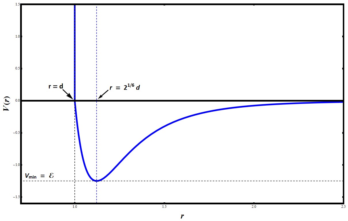
The Mayer function under mean field approximation takes the following form,

$\displaystyle f_{ij}(r)=\begin{cases}-1,&\text{for}\ r<d\\ \exp\left[-\beta{\cal V}(r)\right]-1&\text{for}\ r\geq d,\quad\text{for all}\ i,j.\end{cases}$

(IV.3)

We define a volume $v_{0}$ associated with the critical length $r_{0}$

$$v_{0}=\frac{4\pi}{3}r_{0}^{3}.$$

(IV.4)

Our goal is to compute this volume as a function of temperature and charge and compare the result obtained from the thermodynamic curvature Wei+R.Mann:2019yvs.

Computation of (irreducible) cluster integrals for this potential is in general complicated. To get an analytic handle on the problem we make an approximation to simplify the Mayer function. We assume that $\beta{\cal V}(r)$ is small enough such that the Mayer function can be approximated as

$\displaystyle f_{ij}(r)=\begin{cases}-1,&\text{for}\ r<d\\ -4\beta\varepsilon\left[\left(\frac{d}{r}\right)^{12}-\left(\frac{d}{r}\right)^{6}\right]&\text{for}\ r\geq d,\quad\text{for all}\ i,j.\end{cases}$

(IV.5)

In what follows we see that in the high temperature limit this is a good approximation.

Using (II.6) and (II.11) we can write

$\displaystyle\begin{aligned} \beta_{1}=2\mathchar 22\mkern-9.0mub_{2}&=\frac{1}{V}\iint d^{3}\mathbf{q}_{1}d^{3}\mathbf{q}_{2}f_{ij}(\mathbf{q}_{1},\mathbf{q}_{2})\\ &=-\frac{\beta}{V}\iint d^{3}\mathbf{q}_{1}d^{3}\mathbf{q}_{2}\mathcal{V}(r),\ \text{where}\ r=|\mathbf{q_{1}}-\mathbf{q_{2}}|.\end{aligned}$

(IV.6)

Going to the center of mass frame it is easy to do this integration and the final result is given by,

$$\beta_{1}=\left(-1+\frac{8\varepsilon}{3T}\right)\frac{v_{0}}{\sqrt{2}}.$$

(IV.7)

We first consider a neutral $AdS$ black hole and find the strength of the LJ potential $\varepsilon$ and the critical length $r_{0}$. The second virial coefficient $a_{2}$ for neutral $AdS$ black hole is given by (III.9)

$$a_{2}=-\frac{1}{2\pi T}.$$

(IV.8)

All other higher virial coefficients are zero. Comparing the second virial coefficient with the irreducible cluster integral $\beta_{1}$ one can choose

$$\varepsilon=\frac{3}{8}\left(1+2\sqrt{2}\right)T\sim 1.44\ T$$

(IV.9)

such that $v_{0}$ is given by

$$v_{0}=\frac{1}{2\pi T}.$$

(IV.10)

In the high temperature limit this calculation is quite reliable since higher order irreducible cluster integrals are suppressed by higher powers of $1/T$

$$\beta_{k}\sim\frac{1}{T^{k}}\quad\text{for $k>1$}$$

(IV.11)

and hence the higher virial coefficients.

Thus we see that the LJ potential is a feasible candidate to describe a mean field interaction between the black hole molecules in the high temperature limit. From the potential, we see that the interaction between two molecules is attractive if the specific volume $v$ is greater than the critical volume $v_{0}=1/2\pi T$. The result is in agreement with the result obtained from the computation of the Ruppeiner thermodynamic scalar (see appendix A). From the derivation, one can see that $v_{0}\sim 1/T$ and $\epsilon\sim T$ up to some numerical values. The numerical value for $\epsilon$ can be adjusted such that (IV.10) holds. Therefore from our calculation we see that the LJ potential (IV.1) (up to some numerical factors) suitably describes the interaction between black hole molecules for $AdS$ black holes. In the high temperature limit, the argument of the exponential in (IV.3) goes as

$$\beta{\cal V}(r)\sim\frac{1}{T^{2}}$$

(IV.12)

and hence our approximation $f_{ij}(r)\sim-\beta{\cal V}(r)$ is good enough.

In this article, we probe the effect of electric and magnetic charges on the interaction between black hole molecules by calculating the effective mean-field interaction potential between them using the techniques of classical cluster expansion for a class of $3+1$ dimensional $AdS$ dyonic black holes. The equation of state of charged AdS black hole in the extended phase space is similar to that of a van der Waals fluid. To fully understand the microscopic interactions between the black hole molecules, we take a bottom-up approach to find the mean-field potential between them. It turns out that the Lennard-Jones potential is a feasible choice to explain the interaction between the molecules and it matches with the result obtained by calculating the Ruppeiner thermal curvature.

We first find the LJ potential for a neutral $AdS$ black hole. The computation of irreducible cluster coefficients, in general, is extremely complicated analytically. We consider the high temperature limit and compute these coefficients to find the mean-field potential. It turns out that if we choose the strength of the potential appropriately (the numerical factor), then the critical volume $v_{0}$ becomes $1/2\pi T$. This implies that if the two black hole molecules come in a volume $v_{0}$ they start repelling each other; otherwise, there is an attraction between them. This result is in agreement with Xu:2020sads-rg. Our next goal was to understand what is the effect of the charge parameter $q$ at the microscopic level. Extending our approach for a generic charge parameter is again a formidable task to do. Therefore we make a further approximation. However, this allows us to understand the effect of charge on the microscopic interaction. It turns out that the charge $q$ reduce the size of the critical volume as well as the strength of the LJ potential. Correcting the Mayer (IV.14) function for $r<d$ corresponds to deforming the hard sphere approximation in presence of charges. The interaction potential for $r<d$ goes as $T\log\left(1/q^{2}\right)$. In the limit $q\rightarrow 0$ the potential becomes $\infty$ for $r<d$.

The Ruppeiner curvature scalar for dyonic black holes is given in appendix (equation A.6b). From the expression we see that the curvature has another zero at $v_{0}\sim q^{2}$. Because of this extra zero the characteristic curves studied in Wei:2019uqg is different than the characteristic curves for a van der Waals fluid. However in our analysis we do not see this extra solution for the critical volume $v_{0}$. This is because we studied the charged system as a perturbation over pure $AdS$ black hole. In the limit $q\rightarrow 0$ the second solution is $v_{0}=0$ and it did not show up in our calculation. An exact $q$ calculation might show the second solution for $v_{0}$.

From the microscopic point of view, different virial coefficients (II.9) account for multi-particle interactions. The $n^{th}$ virial coefficient can be calculated from the $n$-body interaction of the micro molecules. From the equation of state of charged $AdS$ black hole (III.9 or III.10) we see that the micro-structure for $AdS$ black hole is potentially different from the standard non-ideal gas. The first term in the equation of state represents the ideal gas part. At a very high temperature ($T\rightarrow\infty$) one can approximate the black hole molecules to be free gas. The second term in the equation implies that at finite temperature, the underlying molecules are not like ideal gas; rather, there is a repulsive two body interaction between them. For a neutral $AdS$ black hole, there are no multi-body interactions between the molecules. Whereas for charged-$AdS$ black hole there is only two body and four-body interactions at the microscopic level where the charge parameter $q$ accounts the strength of the four body interaction. From our analysis, we see that the four body interaction is attractive in the limit of a small charge. The higher order virial coefficients appear under consideration of higher derivative terms in the action in higher dimensions Ghosh:2019pwy; Aman:2005xk; Cvetic:2001bk; Wei:2020poh. It would be interesting to study the effect of higher derivative terms on the interactions between the molecules. Our analysis can also be extended to rotating black holes also. From the temperature of Kerr-AdS black holes one can write the equation of state and read the virial coefficients. It would be interesting to extend this computations for rotating black holes and compare the result with the same from Ruppeiner scalar computation Aman:2005xk; Wei:2021lmo.

Probing the micro-structure via the equation of state does not allow us to count the number of microstates to match with the classical entropy. Consideration of black hole molecules is in some sense ad-hoc. We presume that there exists some microstructure, but we exactly do not know the origin of such states. String theory, on the other hand, has been able to give a partial answer in order to construct the microstructure for macroscopic black holes. However, such black holes solutions are asymptotically flat and have a large amount of supersymmetry in order to compute the indices in the weak coupling limit Strominger:1996sh. An attempt to compute the microstructure for non-extremal black holes can be found in Sfetsos:1997xs; Horowitz:1996ay; Breckenridge:1996sn. Computation of indices of supersymmetric field theories also allows one to understand the underlying microstates for the dual black holes in the context of the $AdS/CFT$ correspondence. It would be interesting to explore if there is any connection between the ad-hoc microstructure for supersymmetric $AdS$ black holes and microstructures computed from supersymmetric indices.

References

- [1] S. W. Hawking. Black Holes and Thermodynamics. Phys. Rev. D, 13:191–197, 1976.
- [2] James M. Bardeen, B. Carter, and S. W. Hawking. The Four laws of black hole mechanics. Commun. Math. Phys., 31:161–170, 1973.
- [3] Jacob D. Bekenstein. Black holes and entropy. Phys. Rev. D, 7:2333–2346, 1973.
- [4] S. W. Hawking. Particle Creation by Black Holes. Commun. Math. Phys., 43:199–220, 1975. Erratum: Commun.Math.Phys. 46, 206 (1976).
- [5] Andrew Strominger and Cumrun Vafa. Microscopic origin of the Bekenstein-Hawking entropy. Phys. Lett. B, 379:99–104, 1996.
- [6] Andrew Chamblin, Roberto Emparan, Clifford V. Johnson, and Robert C. Myers. Charged AdS black holes and catastrophic holography. Phys. Rev. D, 60:064018, 1999.
- [7] Andrew Chamblin, Roberto Emparan, Clifford V. Johnson, and Robert C. Myers. Holography, thermodynamics and fluctuations of charged AdS black holes. Phys. Rev. D, 60:104026, 1999.
- [8] David Kubiznak and Robert B. Mann. P-V criticality of charged AdS black holes. JHEP, 07:033, 2012.
- [9] David Kubiznak and Robert B. Mann. Black hole chemistry. Can. J. Phys., 93(9):999–1002, 2015.
- [10] David Kubiznak, Robert B. Mann, and Mae Teo. Black hole chemistry: thermodynamics with Lambda. Class. Quant. Grav., 34(6):063001, 2017.
- [11] David Kastor, Sourya Ray, and Jennie Traschen. Enthalpy and the Mechanics of AdS Black Holes. Class. Quant. Grav., 26:195011, 2009.
- [12] Yuichi Sekiwa. Thermodynamics of de Sitter black holes: Thermal cosmological constant. Phys. Rev. D, 73:084009, 2006.
- [13] Marco M. Caldarelli, Guido Cognola, and Dietmar Klemm. Thermodynamics of Kerr-Newman-AdS black holes and conformal field theories. Class. Quant. Grav., 17:399–420, 2000.
- [14] Shuang Wang, Shuang-Qing Wu, Fei Xie, and Lin Dan. The First laws of thermodynamics of the (2+1)-dimensional BTZ black holes and Kerr-de Sitter spacetimes. Chin. Phys. Lett., 23:1096–1098, 2006.
- [15] Euro Spallucci and Anais Smailagic. Maxwell’s equal area law for charged Anti-deSitter black holes. Phys. Lett. B, 723:436–441, 2013.
- [16] Natacha Altamirano, David Kubizňák, Robert B. Mann, and Zeinab Sherkatghanad. Kerr-AdS analogue of triple point and solid/liquid/gas phase transition. Class. Quant. Grav., 31:042001, 2014.
- [17] Rong-Gen Cai, Li-Ming Cao, Li Li, and Run-Qiu Yang. P-V criticality in the extended phase space of Gauss-Bonnet black holes in AdS space. JHEP, 09:005, 2013.
- [18] Amin Dehyadegari, Ahmad Sheykhi, and Afshin Montakhab. Critical behavior and microscopic structure of charged AdS black holes via an alternative phase space. Phys. Lett. B, 768:235–240, 2017.
- [19] Shao-Wen Wei and Yu-Xiao Liu. Insight into the Microscopic Structure of an AdS Black Hole from a Thermodynamical Phase Transition. Phys. Rev. Lett., 115(11):111302, 2015. [Erratum: Phys.Rev.Lett. 116, 169903 (2016)].
- [20] George Ruppeiner. Thermodynamics: A riemannian geometric model. Phys. Rev. A, 20:1608–1613, Oct 1979.
- [21] G. Ruppeiner. Thermodynamic Critical Fluctuation Theory? Phys. Rev. Lett., 50:287–290, 1983.
- [22] George Ruppeiner. Riemannian geometry in thermodynamic fluctuation theory. Rev. Mod. Phys., 67:605–659, 1995. [Erratum: Rev.Mod.Phys. 68, 313–313 (1996)].
- [23] Rong-Gen Cai and Jin-Ho Cho. Thermodynamic curvature of the BTZ black hole. Phys. Rev. D, 60:067502, 1999.
- [24] Jan E. Aman, Ingemar Bengtsson, and Narit Pidokrajt. Geometry of black hole thermodynamics. Gen. Rel. Grav., 35:1733, 2003.
- [25] Jan E. Aman and Narit Pidokrajt. Geometry of higher-dimensional black hole thermodynamics. Phys. Rev. D, 73:024017, 2006.
- [26] Jian-yong Shen, Rong-Gen Cai, Bin Wang, and Ru-Keng Su. Thermodynamic geometry and critical behavior of black holes. Int. J. Mod. Phys. A, 22:11–27, 2007.
- [27] Behrouz Mirza and Mohammad Zamani-Nasab. Ruppeiner Geometry of RN Black Holes: Flat or Curved? JHEP, 06:059, 2007.
- [28] Jan E. Åman and Narit Pidokrajt. Ruppeiner Geometry of Black Hole Thermodynamics. EAS Publ. Ser., 30:269–273, 2008.
- [29] Pankaj Chaturvedi, Anirban Das, and Gautam Sengupta. Thermodynamic Geometry and Phase Transitions of Dyonic Charged AdS Black Holes. Eur. Phys. J. C, 77(2):110, 2017.
- [30] Zhen-Ming Xu, Bin Wu, and Wen-Li Yang. Ruppeiner thermodynamic geometry for the Schwarzschild-AdS black hole. Phys. Rev. D, 101(2):024018, 2020.
- [31] Shao-Wen Wei, Yu-Xiao Liu, and Robert B. Mann. Ruppeiner Geometry, Phase Transitions, and the Microstructure of Charged AdS Black Holes. Phys. Rev. D, 100(12):124033, 2019.
- [32] Shao-Wen Wei and Yu-Xiao Liu. Extended thermodynamics and microstructures of four-dimensional charged Gauss-Bonnet black hole in AdS space. Phys. Rev. D, 101(10):104018, 2020.
- [33] Aritra Ghosh and Chandrasekhar Bhamidipati. Thermodynamic geometry for charged Gauss-Bonnet black holes in AdS spacetimes. Phys. Rev. D, 101(4):046005, 2020.
- [34] Amin Dehyadegari, Ahmad Sheykhi, and Shao-Wen Wei. Microstructure of charged AdS black hole via criticality. Phys. Rev. D, 102(10):104013, 2020.
- [35] Yan-Gang Miao and Zhen-Ming Xu. On thermal molecular potential among micromolecules in charged AdS black holes. Phys. Rev. D, 98:044001, 2018.
- [36] K. Huang. STATISTICAL MECHANICS, 2nd edit. Wiley India Pvt. Limited, 2008.
- [37] J.E. Mayer and M.G. Mayer. Statistical Mechanics. J. Wiley & Sons, Incorporated, 1940.
- [38] Mehran Kardar. Statistical Physics of Particles. Cambridge University Press, 2007.
- [39] Suvankar Dutta, Akash Jain, and Rahul Soni. Dyonic Black Hole and Holography. JHEP, 12:060, 2013.
- [40] Guang-Jiun Cheng, Rue-Ron Hsu, and Wei-Fu Lin. Dyonic black holes in string theory. J. Math. Phys., 35:4839–4847, 1994.
- [41] Vijay Balasubramanian and Per Kraus. A Stress tensor for Anti-de Sitter gravity. Commun. Math. Phys., 208:413–428, 1999.
- [42] Shao-Wen Wei, Yu-Xiao Liu, and Robert B. Mann. Repulsive Interactions and Universal Properties of Charged Anti–de Sitter Black Hole Microstructures. Phys. Rev. Lett., 123(7):071103, 2019.
- [43] Mirjam Cvetic, Shin’ichi Nojiri, and Sergei D. Odintsov. Black hole thermodynamics and negative entropy in de Sitter and anti-de Sitter Einstein-Gauss-Bonnet gravity. Nucl. Phys. B, 628:295–330, 2002.
- [44] Shao-Wen Wei and Yu-Xiao Liu. A general thermodynamic geometry approach for rotating Kerr anti-de Sitter black holes. 6 2021.
- [45] Konstadinos Sfetsos and Kostas Skenderis. Microscopic derivation of the Bekenstein-Hawking entropy formula for nonextremal black holes. Nucl. Phys. B, 517:179–204, 1998.
- [46] Gary T. Horowitz, Juan Martin Maldacena, and Andrew Strominger. Nonextremal black hole microstates and U duality. Phys. Lett. B, 383:151–159, 1996.
- [47] J. C. Breckenridge, D. A. Lowe, Robert C. Myers, A. W. Peet, A. Strominger, and C. Vafa. Macroscopic and microscopic entropy of near extremal spinning black holes. Phys. Lett. B, 381:423–426, 1996.
- [48] Suvankar Dutta and P. Sachin Shain. A Mean-Field Description for AdS Black Hole. 6 2016.
- [49] H Janyszek and R Mrugaa. Riemannian geometry and stability of ideal quantum gases. Journal of Physics A: Mathematical and General, 23(4):467–476, feb 1990.
- [50] H Janyszek. Riemannian geometry and stability of thermodynamical equilibrium systems. Journal of Physics A: Mathematical and General, 23(4):477–490, feb 1990.