跳到论文正文
W Papers独立论文阅读器 arXiv:2108.06124 论文正文 计算阅读时间 · 0%
引用这篇论文根据当前论文元数据生成,正式投稿前建议核对。


License: CC BY 4.0
arXiv:2108.06124v1 [quant-ph] 13 Aug 2021

Entanglement Spectrum in General Free Fermionic Systems

Eldad Bettelheim1,2, Aditya Banerjee1, Martin B. Plenio2, Susana F. Huelga2

1:Racah Institute of Physics, Hebrew University of Jerusalem, Edmund J Safta Campus

91904 Jerusalem, Israel

2: Institute of Theoretical Physics and Center for Integrated Quantum Science and Technology (IQST), Universität Ulm, Albert-Einstein-Allee 11, Ulm 89069, Germany.

The statistical mechanics characterization of a finite subsystem embedded in an infinite system is a fundamental question of quantum physics. Nevertheless, a full closed form for all required entropic measures does not exist in the general case even for free systems when the finite system in question is composed of several disjoint intervals. Here we develop a mathematical framework based on the Riemann-Hilbert approach to treat this problem in the one-dimensional case where the finite system is composed of two disjoint intervals and in the thermodynamic limit (both intervals and the space between them contains an infinite number of lattice sites and the result is given as a thermodynamic expansion). To demonstrate the usefulness of our method, we compute the change in the entanglement and negativity namely the spectrum of eigenvalues of the reduced density matrix with our without time reversal of one of the intervals. We do this in the case that the distance between the intervals is much larger than their size. The method we use can be easily applied to compute any power in an expansion in the ratio of the distance between the intervals to their size. We expect these results to provide the necessary mathematical apparatus to address relevant questions in concrete physical scenarios, namely the structure and extent of quantum correlations in fermionic systems subject to local environment.

1 Introduction

A basic concept in statistical physics is the thermodynamics of a subsystem of a larger, often infinite system, the most basic example being perhaps the derivation of the canonical ensemble from the micro-canonical one by taking an infinite system in the micro-canonical ensemble and considering a smaller sub-system, which is then found to be in the canonical ensemble. Nowadays, when applying this procedure to quantum systems and when the thermodynamic potential being investigated in the small system is the entropy, the quantity being measured is brought under the title of ’entanglement entropy’.

Although the newfangled ‘entanglement entropy’ is, in fact, the mundane ‘entropy’ of a sub-region in newer attire, the realization that it is (also) a measure of entanglement allows to focus on aspects previously ignored and for interesting generalizations of the basic quantity [1]. For example, the entropy of the union of several sub-regions may be explored and how it differs from the sum of the individual entropies of the regions may be considered. Another example, comes under the name of ’logarithmic negativity’[2]. For the case of two regions it involves reversing the arrow of time on one sub-region while keeping its direction for the other sub-region and then computing a quantity which is obtained from the entanglement spectrum (to be defined below) of the union of the two sub-regions. The resulting quantity is a measure of entanglement which also is valid for mixed states (in contrast to the entanglement entropy) of the union of the two regions[3, 4, 5, 2].

This manuscript is concerned with the computation of the spectrum of eigenvalues of the reduced density matrix which both in the case in which one applies a partial transpose operation as well as in the case it is not applied in a one dimensional translationally invariant open or closed system of free fermions, from which the logarithmic negativity and entanglement entropy can be computed. These have been computed in the past using numerical methods on bosonic lattice systems [6], field-theoretic techniques[7, 8, 9] and conformal field theory techniques [10, 11]. Closed form results are available when the two sub-systems are adjacent for logarithmic negativity. We therefore investigate here the case where the two sub-systems are not adjacent. It should be noted that the reversal of the time arrow or transposition of the states in one of the regions for fermions has been worked out satisfactorily only recently in Refs. [12, 13]. These references also provide results for the different quantities, but again the two sub-regions are adjacent.

Our approach here is akin to that of Ref. [14], where one starts with the observation that correlation functions within a sub-region are trivially equal to those in the entire region, and that for a free Gaussian system the correlation functions completely dictate the free action that describes the sub-region[15]. From the free Gaussian action of the sub-region, in turn, it is easy to compute the entropy of the sub-region. Note that the Gaussian action of the entire region is necessarily different from one of the sub-region. In field-theoretic language the action of the sub-region is obtained by integrating out the degrees of freedom outside the sub-region. The fact that the correlation function in the sub-region (irrespective of whether we treat it as a sub-system of the large system or as an independent system) obey Wick’s theorem, has two important consequences. The first is that the sub-system must be described by a free Gaussian action, and the second is that it is enough to study the two-point function.

The two point function in a one dimensional single interval can be thought of as a matrix with the indices enumerating the two points involved within the region. The matrix is a Toeplitz matrix since the elements of the matrix depend only on the distance between the two points for a translationally invariant system. Finding the eigenvalues of this matrix provides enough information in order to compute the entropy of that region. To accomplish the latter the authors of Ref. [14] applied the Fisher-Hartwig theorem[16], which gives the determinants of Toeplitz matrices when the size of the matrix is large. A determinant predicts the eigenvalues of a matrix AA by the the usual method of characteristic polynomials. Indeed, one computes det(λ−A)\det(\lambda-A) and searches for the zeros of this determinant. Since for AA a Toeplitz matrix also λ−A\lambda-A is Toeplitz, it is possible to apply the Fisher-Hartwig theorem to compute the characteristic polynomial of AA, namely det(λ−A),\det(\lambda-A), which in turn gives the eigenvalues of AA .

The moment one deals with more than one interval, however, the Toeplitz property of the correlation function is lost. In addition, if one wants to compute the logarithmic negativity of a region, one must apply a certain transformation on the covariance matrix, thereby destroying the Toeplitz property even for adjacent regions. To deal with this situation, we go back to how the Fisher-Hartwig theorem is proved, and try to apply the fundamental methods used to prove the Fisher-Hartwig theorem[17, 18] on the covariance matrix of two regions directly (possibly deforming the covariance matrix appropriately to compute logarithmic negativity), without using a ready-made theorem. The method involved[17, 18, 19] turns out to be the Riemann-Hilbert problem coupled with the orthogonal polynomial technique. It turns out that these methods will allow us to obtain the desired result. Indeed, the Riemann-Hilbert problem associated with finding the determinant of a Toeplitz matrix (thus producing the Fisher-Hartwig theorem), is closely related to the Riemann-Hilbert problem that we shall solve here, as both are solved in terms of confluent hypergeometric functions[19].

We dedicate this paper to the technical aspects of the computation, whereby we show how to map the problem of entanglement characterisation into a Riemann-Hilbert problem, and plan to apply the method to obtain more physical results in a following publication. Nevertheless, we give here some results as well, notably Eqs. (7.48-7.49), the entanglement and negativity spectra to leading order in the ratio between the size of the intervals and their distance.

2 Open and Closed Free Fermion Systems on a Line

We consider a fermionic free field theory, described by a fermionic field operator cic_{i} at site ii, each coupled to a reservoir comprised of NN fermionic modes. These modes are labeled by the fermionic operator an,ia_{n,i} where nn labels the mode number 1≤n≤N1\leq n\leq N and ii labels the site (see Fig. 1 for a pictorial representation of the physical situation). The Hamiltonian of the system is given by

H=−∑iℏ22​M​a2ci†(ci+1+ci−1−2ci)+α∑i,nHnℏΔ(ci†an,i+cian,i†)+\displaystyle H=-\sum_{i}\frac{\hbar^{2}}{2Ma^{2}}c^{\dagger}_{i}(c_{i+1}+c_{i-1}-2c_{i})+\alpha\sum_{i,n}H_{n}\hbar\sqrt{\Delta}(c^{\dagger}_{i}a_{n,i}+c_{i}a^{\dagger}_{n,i})+ (2.1)
+∑i,nℏGna†n,ian,i,\displaystyle+\sum_{i,n}\hbar G_{n}a^{\dagger}_{n,i}a_{n,i}, (2.2)

where

Gn=Δ​n+ω<,ℏ​w>=ℏ​Δ​N+ℏ​ω<,\displaystyle G_{n}=\Delta n+\omega_{<},\quad\hbar w_{>}=\hbar\Delta N+\hbar\omega_{<}, (2.3)

and ω<\omega_{<} and ω>\omega_{>} are the band edges of the reservoir. The quantity Δ\Delta represents the level spacing of the Reservoir, and HnH_{n} is a coupling constant, with an arbitrary dependence on nn. One obtains the following equations for the field variables:

ı​ℏ​∂tci=ℏ22​M​a2​(ci+1+ci−1−2​ci)−∑nα​an,i​Hn​ℏ​Δ\displaystyle\imath\hbar\partial_{t}c_{i}=\frac{\hbar^{2}}{2Ma^{2}}(c_{i+1}+c_{i-1}-2c_{i})-\sum_{n}\alpha a_{n,i}H_{n}\hbar\sqrt{\Delta}\ (2.4)
ı​ℏ​∂tan,i=−an,i​ℏ​Gn−α​ci​Hn​ℏ​Δ\displaystyle\imath\hbar\partial_{t}a_{n,i}=-a_{n,i}\hbar G_{n}-\alpha c_{i}H_{n}\hbar\sqrt{\Delta} (2.5)
Refer to caption
Figure 1: A system of Fermions described by the fermionic annihilation operator cic_{i} of LL sites are coupled to each other by nearest neighbour interaction (heavy lines). In addition, each fermion at site ii is coupled locally to NN fermionic modes ai,n,a_{i,n}, with nn running from 11 to NN. The gray rectangular boxes denote that the fermions contained in a given box interact with each other.

Now Fourier transform both in time and in space according to the following transformation rule

g⁡(z,ω)=12​π​∑jzj​∫d​t​gj​(t)​e−ı​ω​t\displaystyle g(z,\omega)=\frac{1}{2\pi}\sum_{j}z^{j}\int dtg_{j}(t)e^{-\imath\omega t} (2.6)

yields the following equations of motion for the Fourier transformed field operators:

(z+z−1−22​ℏ−2​M​a2+ℏ​ω)​c​(z,ω)−α​∑nan​(z,ω)​Hn​ℏ​Δ=0\displaystyle\left(\frac{z+z^{-1}-2}{2\hbar^{-2}Ma^{2}}+\hbar\omega\right)c(z,\omega)-\alpha\sum_{n}a_{n}(z,\omega)H_{n}\hbar\sqrt{\Delta}=0 (2.7)
ℏ​ω​an​(z,ω)−ℏ​Gn​an​(z,ω)−α​c​(z,ω)​Hn​ℏ​Δ=0.\displaystyle\hbar\omega a_{n}(z,\omega)-\hbar G_{n}a_{n}(z,\omega)-\alpha c(z,\omega)H_{n}\hbar\sqrt{\Delta}=0. (2.8)

Thus,

(z+z−1−22​ℏ−2​M​a2+ℏ​ω)​c​(z,ω)−α2​c​(z,ω)​∑nHn2​ℏ​Δω−Gn=0,\displaystyle\left(\frac{z+z^{-1}-2}{2\hbar^{-2}Ma^{2}}+\hbar\omega\right)c(z,\omega)-\alpha^{2}c(z,\omega)\sum_{n}\frac{H_{n}^{2}\hbar\Delta}{\omega-G_{n}}=0, (2.9)

Thus we have the dispersion relation:

ℏ​ω=ε⁡(p)+α~​(ω),\displaystyle\hbar\omega=\varepsilon(p)+\tilde{\alpha}(\omega), (2.10)

where

ε⁡(p)=ℏ2M​a2​(1−cos⁡(p)),z=eı​p,\displaystyle\varepsilon(p)=\frac{\hbar^{2}}{Ma^{2}}(1-\cos(p)),\quad z=e^{\imath p}, (2.11)

and

α~​(ω)=ℏ​α2​Δ​∑nHn2ω−Gn.\displaystyle\tilde{\alpha}(\omega)=\hbar\alpha^{2}\Delta\sum_{n}\frac{H_{n}^{2}}{\omega-G_{n}}. (2.12)

The eigenvectors that leads to the eigenvalue ℏ​ω\hbar\omega are formally obtained by solving Eq. (2.8) to yield:

an​(z,ω)=α​Hn​Δω−Gn​c​(z,ω).\displaystyle a_{n}(z,\omega)=\frac{\alpha H_{n}\sqrt{\Delta}}{\omega-G_{n}}c(z,\omega). (2.13)

Thus the combination

c~ω​(z,t)=1Cω​(c⁡(z,t)+Δ​α​∑nHn​an​(z,t)ω−Gn)\displaystyle\tilde{c}_{\omega}(z,t)=\frac{1}{C_{\omega}}\left(c(z,t)+\sqrt{\Delta}\alpha\sum_{n}\frac{H_{n}a_{n}(z,t)}{\omega-G_{n}}\right) (2.14)

where

Cω=1+Δ​α2​∑nHn2(ω−Gn)2\displaystyle C_{\omega}=\sqrt{1+\Delta\alpha^{2}\sum_{n}\frac{H^{2}_{n}}{(\omega-G_{n})^{2}}} (2.15)

satisfies:

ı​ℏ​∂tc~ω​(z,t)=−ℏ​ω​c~ω​(z,t),{c~ω​(z,t),c~ω†​(z,t)}=1.\displaystyle\imath\hbar\partial_{t}\tilde{c}_{\omega}(z,t)=-\hbar\omega\tilde{c}_{\omega}(z,t),\quad\{\tilde{c}_{\omega}(z,t),\tilde{c}^{\dagger}_{\omega}(z,t)\}=1.

Numbering all the solution of the dispersion for given zz by ωj\omega_{j}, where 1≤j≤N+11\leq j\leq N+1, we have:

c⁡(z,t)=∑jc~ωj​(z,t)Cωj,\displaystyle c(z,t)=\sum_{j}\frac{\tilde{c}_{\omega_{j}}(z,t)}{C_{\omega_{j}}}, (2.16)

so that, after dropping the time variable due to the trivial time dependence, one obtains:

⟨c†​(z)​c​(z)⟩=∑j⟨c~ωj†​(z)​c~ωj​(z)⟩Cωj2.\displaystyle\langle c^{\dagger}(z)c(z)\rangle=\sum_{j}\frac{\langle\tilde{c}^{\dagger}_{\omega_{j}}(z)\tilde{c}_{\omega_{j}}(z)\rangle}{C^{2}_{\omega_{j}}}. (2.17)

Now, in the ground state of the entire system, which includes both the reservoir and the fermionic system. All states, enumerated by ωj​(p),\omega_{j}(p), with energy ℏ​ωj​(p)\hbar\omega_{j}(p) below a certain energy, called the Fermi energy and denoted by ϵF,\epsilon_{F}, are occupied ⟨c~ωj†​(z)​c~ωj​(z)⟩=1\langle\tilde{c}^{\dagger}_{\omega_{j}}(z)\tilde{c}_{\omega_{j}}(z)\rangle=1 and all those above are unoccupied, ⟨c~ωj†​(z)​c~ωj​(z)⟩=0,\langle\tilde{c}^{\dagger}_{\omega_{j}}(z)\tilde{c}_{\omega_{j}}(z)\rangle=0, and as such we have:

⟨c†​(z)​c​(z)⟩=∑jθ⁡(ℏ​ωj​(p)<ϵF)Cωj2\displaystyle\langle c^{\dagger}(z)c(z)\rangle=\sum_{j}\frac{\theta(\hbar\omega_{j}(p)<\epsilon_{F})}{C^{2}_{\omega_{j}}} (2.18)

From Eq. (2.10) and (2.15) one can see

Cω2=|1ℏ​d​ε​(p)d​ω|,\displaystyle C_{\omega}^{2}=\left|\frac{1}{\hbar}\frac{d\varepsilon(p)}{d\omega}\right|, (2.19)

then Eq. (2.11) yields:

Cω2=ℏ​|sin⁡(p)|m​a2​|ω′​(p)|\displaystyle C_{\omega}^{2}=\frac{\hbar|\sin(p)|}{ma^{2}|\omega^{\prime}(p)|} (2.20)

Such that:

⟨c†​(p)​c​(p)⟩=∑j|ℏ​ωj′​(p)||ℏ​ω¯′​(p)|​θ​(ℏ​ωj​(p)<ϵF),\displaystyle\langle c^{\dagger}(p)c(p)\rangle=\sum_{j}\frac{|\hbar\omega_{j}^{\prime}(p)|}{|\hbar\bar{\omega}^{\prime}(p)|}\theta(\hbar\omega_{j}(p)<\epsilon_{F}), (2.21)

where

|ℏ​ω¯′​(p)|≡ℏ2m​a2​|sin⁡(p)|.\displaystyle|\hbar\bar{\omega}^{\prime}(p)|\equiv\frac{\hbar^{2}}{ma^{2}}|\sin(p)|. (2.22)

We now discuss the continuum limit of the dispersion relation. The function α~​(ω)\tilde{\alpha}(\omega) can be written in the continuum limit (N→∞,N\to\infty, Δ∼1/N\Delta\sim 1/N) as follows:

α~(ω)=ℏα2(−∫ω<ω>H2​(Ω)ω−ΩdΩ+δ(ω)),\displaystyle\tilde{\alpha}(\omega)=\hbar\alpha^{2}\left(\mathchoice{{\vbox{\hbox{$\textstyle-$}}\kern-4.86108pt}}{{\vbox{\hbox{$\scriptstyle-$}}\kern-3.43057pt}}{{\vbox{\hbox{$\scriptscriptstyle-$}}\kern-2.908pt}}{{\vbox{\hbox{$\scriptscriptstyle-$}}\kern-2.76045pt}}\!\int_{\omega_{<}}^{\omega_{>}}\frac{H^{2}(\Omega)}{\omega-\Omega}d\Omega+\delta(\omega)\right), (2.23)

where the integral is the Cauchy principal value integral and H⁡(Ω)H(\Omega) is an interpolating function of HnH_{n}:

H⁡(Gn)≡Hn,\displaystyle H(G_{n})\equiv H_{n}, (2.24)

while δ⁡(ω)\delta(\omega) (not to be confused with Kronecker’s delta) is a function that appears when taking the continuum limit, N→∞,N\to\infty, Δ∼1/N,\Delta\sim 1/N, of Eq. (2.12). The function depends on the microscopic location of ω\omega within the reservoir frequencies, GnG_{n}, and is given by:

δ⁡(ω)={π​H2​(ω)​cot⁡(ω−ω<)​πΔω∈[ω<,ω>],|ω−ω<,>|≫Δ0ω∉[ω<,ω>],|ω−ω<,>|≫Δ.\displaystyle\delta(\omega)=\left\{\begin{array}[]{lr}\pi H^{2}(\omega)\cot\frac{(\omega-\omega_{<})\pi}{\Delta}&\omega\in[\omega_{<},\omega_{>}],\quad|\omega-\omega_{<,>}|\gg\Delta\\ 0&\omega\notin[\omega_{<},\omega_{>}],\quad|\omega-\omega_{<,>}|\gg\Delta\end{array}\right..

The N+1N+1 solutions of the dispersion relation, Eq. (2.10) in the small α\alpha limit, are composed of NN perturbed reservoir energy levels and 11 perturbed non-reservoir fermionic level. If, for example, the reservoir is above the unperturbed Fermi sea, ϵF<ℏ​ω<<ℏ​ω>,\epsilon_{F}<\hbar\omega_{<}<\hbar\omega_{>}, the perturbed reservoir energies will typically also lie above the Fermi sea. In this case only the perturbed energy of the non-reservoir fermion will lie under the Fermi sea. Since this state is below the reservoir δ⁡(ω)=0\delta(\omega)=0 must be set in Eq. (2.23). One can then have that only the perturbed non-reservoir level lies below the Fermi energy ϵF\epsilon_{F}. This leads to the following form for the fermionic occupation:

⟨c†​(p)​c​(p)⟩=f⁡(eı​p)+12,f⁡(eı​p)=−1​ for ​|p|>pF\displaystyle\langle c^{\dagger}(p)c(p)\rangle=\frac{f(e^{\imath p})+1}{2},\quad f(e^{\imath p})=-1\mbox{ for }|p|>p_{F} (2.27)

where f⁡(eı​p)f(e^{\imath p}) is an arbitrary function of pp for |p|<pF|p|<p_{F}. The Fermi momentum pFp_{F} is defined as the momentum for which the dispersion relation, Eq. (2.10), is solved with ω=ωF≡ϵF/ℏ\omega=\omega_{F}\equiv\epsilon_{F}/\hbar:

ℏ​ωF=ε⁡(pF)+α~​(ωF),\displaystyle\hbar\omega_{F}=\varepsilon(p_{F})+\tilde{\alpha}(\omega_{F}), (2.28)

More generally, it is easy then to find different models of the reservoir, defined by different values of Hn,H_{n}, ω<\omega_{<}, ω>\omega_{>} and Δ\Delta such that Eq. (2.27) holds. The Fermi momentum, pF,p_{F}, is defined such as that the solution with δ⁡(ω)=0\delta(\omega)=0 of (2.10) exists with p=pFp=p_{F} and ℏ​ω=ϵF\hbar\omega=\epsilon_{F}. The combination f⁡(eı​p)+12\frac{f(e^{\imath p})+1}{2} is chosen for later convenience.

Other possibilities of course exist generalizing Eq. (2.27), where the distribution inside and outside the Fermi sea is arbitrary, but we shall not try to describe the reservoirs leading to such distribution here for the sake of brevity. The problem of finding such reservoirs was treated in other works [20, 21]. We note that although for our choice of reservoir above the Fermi sea, the specific functional form of the coupling function H⁡(ω)H(\omega) plays little role, in other cases this function may introduce singularities into the ferminic occupation number and thus play a more crucial role in determining the behavior of entanglement in the system. What is rather general is that there is a jump discontinuity in the value of ⟨c†​(p)​c​(p)⟩.\langle c^{\dagger}(p)c(p)\rangle. This is the general case if |ℏ​ωj′​(p)|≠0.|\hbar\omega_{j}^{\prime}(p)|\neq 0. If |ℏ​ωj′​(p)|=0,|\hbar\omega_{j}^{\prime}(p)|=0, one the other hand, a power-law behavior around the Fermi momenutm rather than a jump discontinuity occurs. We shall treat here the problem where the behavior around the Fermi point is of a jump discontinuity.

To simplify the analysis later on we shall assume that the two Fermi points, ±pF\pm p_{F} are symmetric, namely:

f⁡(eı⁡(pF+δ​p))=f⁡(eı⁡(−pF−δ​p)),\displaystyle f(e^{\imath(p_{F}+\delta p)})=f(e^{\imath(-p_{F}-\delta p)}), (2.29)

which can be more succinctly written as:

f⁡(z)=f⁡(z−1).\displaystyle f(z)=f(z^{-1}). (2.30)

3 Entanglement Entropy and Negativity

We consider a translationally invariant Gaussian fermionic systems with density matrix

ρ=1Z​e∑i​jΩi​j​ci†​cj,tr​ρ=1\displaystyle\rho=\frac{1}{Z}e^{\sum_{ij}\Omega_{ij}c^{\dagger}_{i}c_{j}},\,{\rm tr}\rho=1 (3.1)

on the infinite line. The covariance matrix fi−jf_{i-j} is defined by:

fi−j=tr⁡((2​ρ−𝟙)​ci†​cj),\displaystyle f_{i-j}={\rm tr}\left((2\rho-\mathds{1})c^{\dagger}_{i}c_{j}\right), (3.2)

which leads naturally to define the symbol f⁡(z)f(z), namely the generating function for fi−jf_{i-j}:

f⁡(z)=∑ifi​zi.\displaystyle f(z)=\sum_{i}f_{i}z^{i}. (3.3)

Note that this definition leads to the following expression for the average occupation fermionic occupation number, ⟨c†​(p)​c​(p)⟩,\langle c^{\dagger}(p)c(p)\rangle, as a function of momentum, pp:

⟨c†​(p)​c​(p)⟩≡tr⁡(ρ​c†​(p)​c​(p))=f⁡(eı​p)+12,\displaystyle\langle c^{\dagger}(p)c(p)\rangle\equiv{\rm tr}\left(\rho c^{\dagger}(p)c(p)\right)=\frac{f(e^{\imath p})+1}{2}, (3.4)

conforming with Eq. (2.27). We must deal then with the problem of f⁡(p)f(p) having a jump discontinuity, due to the presence of a Fermi surface, where namely a momentum p=pFp=p_{F} at which the function f⁡(eı​p)f(e^{\imath p}) jumps (for higher dimensions the dimensionality of the Fermi surface also plays an important role, see Ref. [22]).

The density matrix and the covariance matrix are of course related to each other. The density matrix may be diagonalized in a multi-particle basis based on a single-particle basis that diagonlizes the covariance matrix. We get an eigenvalue of the density matrix for every choice of whether a fermion occupies one of the fermionic eigenstates, that diagonalize the covariance matrix [15]. Thus if there are NN eigenvalues of the covariance matrix one finds 2N2^{N} eigenvalues of the density matrix. Specifically, if λi\lambda_{i} are the NN eigenvalues of the covariance matrix, then for any choice of NN values for νi\nu_{i}, where νi∈{1+λi2,1−λi2}\nu_{i}\in\{\frac{1+\lambda_{i}}{2},\frac{1-\lambda_{i}}{2}\} (corresponding to the choice of occupied and unoccupied fermionic states, respectively), there will correspond an eigenvalue of the density matrix, ρ,\rho, of the form:

∏iνi.\displaystyle\prod_{i}\nu_{i}. (3.5)

Despite of the fact that the eigenvalues of the density matrix are the products of the νi\nu_{i}, we shall refer, in a somewhat loose manner, to the individual values of νi,\nu_{i}, as the ‘eigenvalues of the density matrix’ and denote them, as we have just done, by νi\nu_{i}. The spectrum of νi\nu_{i} is known as the entanglement spectrum, and is related to the spectrum of λi\lambda_{i} as follows:

±λi=2​νi−1.\displaystyle\pm\lambda_{i}=2\nu_{i}-1. (3.6)

The ±\pm sign allows one to obtain both eigenvalues of the density matrix, νi\nu_{i} and 1−νi,1-\nu_{i}, from the same value of λi\lambda_{i}. If the spectrum of the covariance matrix, λi\lambda_{i}, is known, or equivalently, the entanglement spectrum, νi,\nu_{i},is known, then the entropy of the system may be computed through

S=∑iνi​log⁡(νi)+(1−νi)​log⁡(1−νi)=∑i1+λi2​log​1+λi2+1−λi2​log​1−λi2.\displaystyle S=\sum_{i}\nu_{i}\log(\nu_{i})+(1-\nu_{i})\log(1-\nu_{i})=\sum_{i}\frac{1+\lambda_{i}}{2}\log\frac{1+\lambda_{i}}{2}+\frac{1-\lambda_{i}}{2}\log\frac{1-\lambda_{i}}{2}. (3.7)

Translational invariance makes the Fourier transform f⁡(z)f(z) of the correlation function fi−jf_{i-j} a very convenient object to work with. Indeed, for any linear combination of fermionic operators c(a)=∑ai​cic^{(a)}=\sum a_{i}c_{i} one forms the function g(a)​(z)=∑ai​z−ig^{(a)}(z)=\sum a_{i}z^{-i} and one easily obtains:

h(a)​(z)≡∑izi​tr​((𝟙−2​ρ)​ci†​c(a))=f⁡(z)​g(a)​(z).\displaystyle h^{(a)}(z)\equiv\sum_{i}z^{i}{\rm tr}\left((\mathds{1}-2\rho)c^{\dagger}_{i}c^{(a)}\right)=f(z)g^{(a)}(z). (3.8)

h(a)h^{(a)} encodes as a Fourier transform the correlation function of c(a)c^{(a)} with any fermionic operator ci†c^{\dagger}_{i}. We see that ff acts in a simple multiplicative fashion on g(a)g^{(a)} to yield h(a)h^{(a)}, which is of great convenience.

Refer to caption
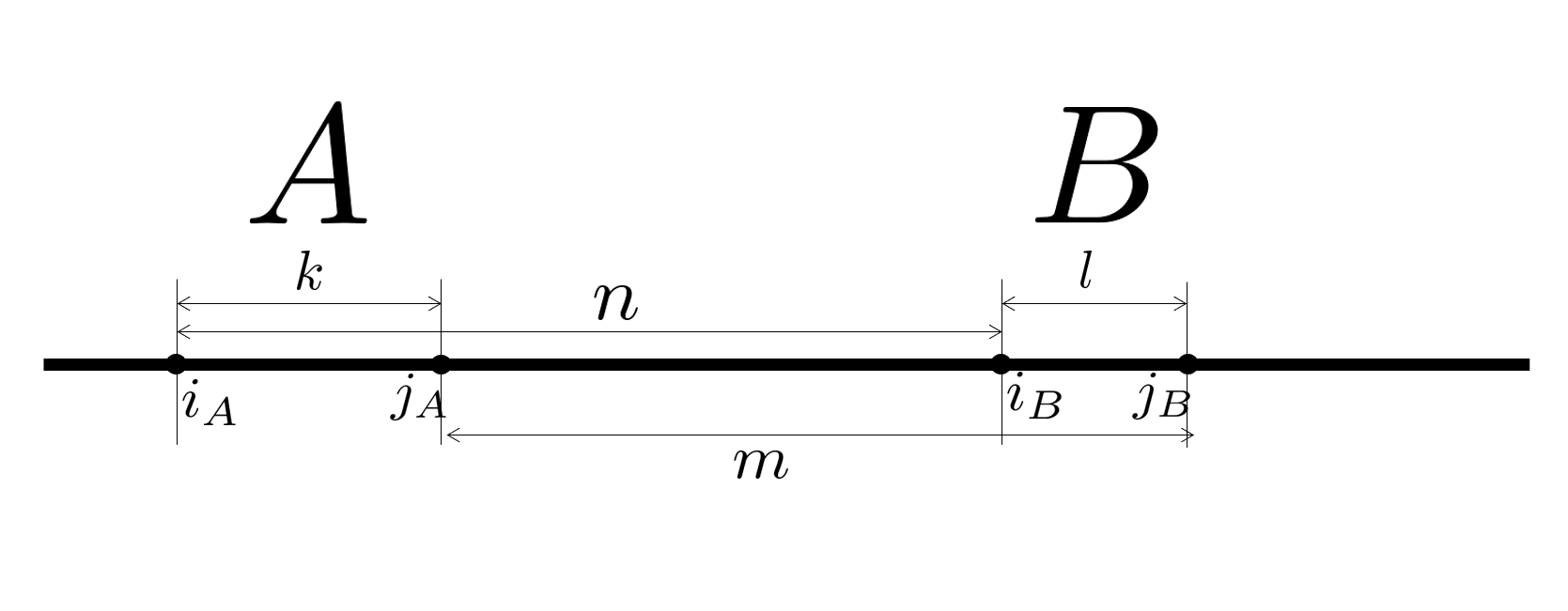
Figure 2: Two subsystems AA and BB are identified on the 1 dimensional real line (heavy line). The size of AA is k+1k+1 and its endpoints are iAi_{A} and jAj_{A} while the size of BB is l+1l+1 and its endpoints are iBi_{B} and jBj_{B}. The distance nn is defined as n=iB−iAn=i_{B}-i_{A} while mm is defined as jB−jAj_{B}-j_{A}.

Take now two intervals AA and BB on the infinite line as shown in Fig. 2, with AA to the left of BB. Let k+1k+1 be the size of AA and l+1l+1 be the size of BB and the distance between the leftmost point of AA and the leftmost point of BB being nn. Let iAi_{A} bet the leftmost point in AA and iBi_{B} be the leftmost point in BB. Define also:

kj=j−{iAj∈AiBk∈B.\displaystyle k_{j}=j-\left\{\begin{array}[]{lr}i_{A}&j\in A\\ i_{B}&k\in B\end{array}\right..

We now write an analogue to Eq. (3.8). To this aim first take any fermionic operator c(a​b)=c(a)+c(b)c^{(ab)}=c^{(a)}+c^{(b)} where c(a)c^{(a)} is a linear combination of fermionic operators in AA and c(b)c^{(b)} is a linear combination of fermionic operators in B:B:

c(a)=∑j∈Aaj(a)​cj,c(b)=∑j∈Baj(b)​cj.\displaystyle c^{(a)}=\sum_{j\in A}a^{(a)}_{j}c_{j},\quad c^{(b)}=\sum_{j\in B}a^{(b)}_{j}c_{j}. (3.11)

Now define gm(a​b)g_{m}^{(ab)} where m=1,2m=1,2 as:

g1(a​b)=∑j∈Aaj(a)​z−kj,\displaystyle g_{1}^{(ab)}=\sum_{j\in A}a^{(a)}_{j}z^{-k_{j}}, (3.12)
g2(a​b)=∑j∈Baj(b)​z−kj.\displaystyle g_{2}^{(ab)}=\sum_{j\in B}a^{(b)}_{j}z^{-k_{j}}. (3.13)

We wish to find the correlator of c(a​b)c^{(ab)} with any fermionic operator in AA or in BB. To this aim we define h1(a​b),h_{1}^{(ab)}, h2(a​b)h_{2}^{(ab)} that encode these correlators as a Fourier transform:

h1(a​b)​(z)≡∑izi−iA​tr​((𝟙−2​ρ)​ci†​c(a)),\displaystyle h_{1}^{(ab)}(z)\equiv\sum_{i}z^{i-i_{A}}{\rm tr}\left((\mathds{1}-2\rho)c^{\dagger}_{i}c^{(a)}\right), (3.14)
h2(a​b)​(z)≡∑izi−iB​tr​((𝟙−2​ρ)​ci†​c(b)).\displaystyle h_{2}^{(ab)}(z)\equiv\sum_{i}z^{i-i_{B}}{\rm tr}\left((\mathds{1}-2\rho)c^{\dagger}_{i}c^{(b)}\right). (3.15)

Then one has the following relations:

h1(a​b)​(z)=f⁡(z)​g1(a​b)+f⁡(z)​zn​g2(a​b)\displaystyle h^{(ab)}_{1}(z)=f(z)g^{(ab)}_{1}+f(z)z^{n}g_{2}^{(ab)} (3.16)
h2(a​b)​(z)=f⁡(z)​z−n​g1(a​b)+f⁡(z)​g2(a​b).\displaystyle h^{(ab)}_{2}(z)=f(z)z^{-n}g^{(ab)}_{1}+f(z)g_{2}^{(ab)}. (3.17)

These can be written in matrix form:

𝒉(a​b)=𝒇​𝒈(a​b),𝒇⁡(z)=(f⁡(z)f⁡(z)​znf⁡(z)​z−nf⁡(z)).\displaystyle\bm{h}^{(ab)}=\bm{f}{\bm{g}}^{(ab)},\quad\bm{f}(z)=\begin{pmatrix}f(z)&f(z)z^{n}\\ f(z)z^{-n}&f(z)\\ \end{pmatrix}. (3.18)

The first equation here is the generalization of Eq. (3.8) that we seek, where ff is replaced by the matrix 𝒇\bm{f}. Thus, 𝒇\bm{f} will be the object describing the correlations within and between the two regions AA and BB.

One may look for the reduced density matrix namely a Gaussian matrix ρA​B\rho^{AB} such that for any i,j∈A∪Bi,j\in A\cup B

tr​ρA​B​ci†​cj=tr​ρ​ci†​cj,ρA​B=1ZA​B​e∑i,j∈A∪BΩi​jA​B​ci†​cj,tr​ρA​B=1.\displaystyle{\rm tr}\rho^{AB}c_{i}^{\dagger}c_{j}={\rm tr}\rho c^{\dagger}_{i}c_{j},\quad\rho^{AB}=\frac{1}{Z^{AB}}e^{\sum_{i,j\in A\cup B}\Omega^{AB}_{ij}c^{\dagger}_{i}c_{j}},\quad{\rm tr}\rho^{AB}=1. (3.19)

Since the right hand side of the first equation is determined by fi−jf_{i-j} restricted on A∪BA\cup B and the left hand side by ΩA​B\Omega^{AB}, the problem reduces to finding ΩA​B\Omega^{AB} given fi−jf_{i-j}. In fact, both matrices are diagonalized in the same basis, and there is a simple relation between their eigenvalues, Eq. (3.6) still holds. The matrix fi−jf_{i-j} restricted to A∪BA\cup B is in turn encoded in 𝒇\bm{f}. An eigenfunction 𝝍(−λ)\bm{\psi}^{(-\lambda)} with eigenvalue −λi(k​l),-\lambda^{(kl)}_{i}, where i=1,2,…,k+li=1,2,\dots,k+l solves the following equation:

𝒫k​l​(𝒇+λi(k​l)​𝟙)​𝝍(−λi(k​l))=0,\displaystyle\mathcal{P}_{kl}(\bm{f}+\lambda_{i}^{(kl)}\mathds{1})\bm{\psi}^{(-\lambda^{(kl)}_{i})}=0, (3.20)

where 𝒫k​l\mathcal{P}_{kl} is the projection operator onto A∪BA\cup B:

𝒫k​l​∑i(𝒂𝟏​𝒊​𝒛𝒊𝒂𝟐​𝒊​𝒛𝒊)=(∑0≤i<|A|a1​i​zi∑0≤i<|B|a2​i​zi)\displaystyle\mathcal{P}_{kl}\sum_{i}\bm{\left}(\begin{array}[]{c}a_{1i}z^{i}\\ a_{2i}z^{i}\end{array}\right)=\left(\begin{array}[]{c}\sum_{0\leq i<|A|}a_{1i}z^{i}\\ \sum_{0\leq i<|B|}a_{2i}z^{i}\end{array}\right)

and 𝝍(−λ)\bm{\psi}^{(-\lambda)} is in A∪BA\cup B, namely 𝒫k​l​𝝍(−λ)=𝝍(−λ)\mathcal{P}_{kl}\bm{\psi}^{(-\lambda)}=\bm{\psi}^{(-\lambda)}. This requires ψ1\psi_{1} and ψ2\psi_{2} to be polynomials of degree |A|−1|A|-1 and |B|−1|B|-1 respectively. So, in effect, one searches for orthogonal polynomials with respect to the measure 𝒇\bm{f}. Once the eigenvalues are found, the eigenvalues νi(k​l)\nu_{i}^{(kl)} of ΩA​B\Omega^{AB} follow from Eq. (3.6), repeated here for completion:

±λi(k​l)=2​νi(k​l)−1.\displaystyle\pm\lambda^{(kl)}_{i}=2\nu^{(kl)}_{i}-1. (3.25)

Then for example, the reduced or entanglement entropy of the region A​BAB can then be computed as follows:

SA​B=∑i1+λi(k​l)2​log⁡1+λi(k​l)2+1−λi(k​l)2​log⁡1−λi(k​l)2.\displaystyle S^{AB}=\sum_{i}\frac{1+\lambda^{(kl)}_{i}}{2}\log\frac{1+\lambda^{(kl)}_{i}}{2}+\frac{1-\lambda^{(kl)}_{i}}{2}\log\frac{1-\lambda^{(kl)}_{i}}{2}. (3.26)

As mentioned in the introduction one may wish to compute the negativity spectrum. In this case one replaces the covariance matrix fki,kjf_{k_{i},k_{j}} by a deformed covariance matrix f~ki,kj\tilde{f}_{k_{i},k_{j}}[12, 13]:

f~ki,kj=tr⁡((𝟙−2​ρ)​ci†​cj)×{1i∈A,j∈A−1i∈B,j∈Bii∈A,j∈Bii∈B,j∈A.\displaystyle\tilde{f}_{k_{i},k_{j}}={\rm tr}\left((\mathds{1}-2\rho)c^{\dagger}_{i}c_{j}\right)\times\left\{\begin{array}[]{lr}1&i\in A,j\in A\\ -1&i\in B,j\in B\\ i&i\in A,j\in B\\ i&i\in B,j\in A\\ \end{array}\right..

The problem is to find ρ~A​B\tilde{\rho}^{AB} such that

f~ki,kj=tr⁡((𝟙−2​ρ~A​B)​ci†​cj),ρ~A​B=1Z~A​B​e∑i,j∈A∪BΩ~i,jA​B​ci†​cj,tr​ρ~A​B=1.\displaystyle\tilde{f}_{k_{i},k_{j}}={\rm tr}\left((\mathds{1}-2\tilde{\rho}^{AB})c^{\dagger}_{i}c_{j}\right),\quad\tilde{\rho}^{AB}=\frac{1}{\tilde{Z}^{AB}}e^{\sum_{i,j\in A\cup B}\tilde{\Omega}^{AB}_{i,j}c^{\dagger}_{i}c_{j}},\quad{\rm tr}\tilde{\rho}^{AB}=1. (3.31)

An eigenfunction 𝝍(−λ~i(k​l))\bm{\psi}^{(-\tilde{\lambda}^{(kl)}_{i})} with eigenvalue −λ~i(k​l)-\tilde{\lambda}_{i}^{(kl)} solves the following equation:

𝒫k​l​(𝒇~+λ~i(k​l)​𝟙)​𝝍(−λ~i(k​l))=0,\displaystyle\mathcal{P}_{kl}(\tilde{\bm{f}}+\tilde{\lambda}_{i}^{(kl)}\mathds{1})\bm{\psi}^{(-\tilde{\lambda}^{(kl)}_{i})}=0, (3.32)

where, in accordance with Eq. (3), one has:

𝒇~​(z)=(f⁡(z)ı​f​(z)​znı​f​(z)​z−n−f⁡(z)).\displaystyle\tilde{\bm{f}}(z)=\begin{pmatrix}f(z)&\imath f(z)z^{n}\\ \imath f(z)z^{-n}&-f(z)\\ \end{pmatrix}. (3.33)

Once the roots of Eq. (3.32) are found one may find the negativity spectrum through:

±λ~i(k​l)=2​ν~i(k​l)−1.\displaystyle\pm\tilde{\lambda}^{(kl)}_{i}=2\tilde{\nu}^{(kl)}_{i}-1. (3.34)

The logarithmic negativity, written using the symbol ℰ\mathcal{E} may be used as a potential that quantifies the entanglement of the system[23]. It is computed by considering only negative values of ρ~A​B\tilde{\rho}^{AB} and computing the sum of the logarithm of only those eigenvalues:

ℰ=∑ilog⁡(|ν~i|+|1−ν~i|)=∑ilog⁡(|1−λ~i2|+|1+λ~i2|)=∑{i||λ~i|>1}log⁡|λ~i|.\displaystyle\mathcal{E}=\sum_{i}\log(\left|\tilde{\nu}_{i}\right|+\left|1-\tilde{\nu}_{i}\right|)=\sum_{i}\log\left(\left|\frac{1-\tilde{\lambda}_{i}}{2}\right|+\left|\frac{1+\tilde{\lambda}_{i}}{2}\right|\right)=\sum_{\{i||\tilde{\lambda}_{i}|>1\}}\log|\tilde{\lambda}_{i}|. (3.35)

Indeed, if both ν~i\tilde{\nu}_{i} and 1−ν~i1-\tilde{\nu}_{i} are positive, the sum, |ν~i|+|1−ν~i|,\left|\tilde{\nu}_{i}\right|+\left|1-\tilde{\nu}_{i}\right|, just gives 11 and the contribution (after taking the logarithm) of the term associated with his expression in the sum after the first equality sign cancels leading to the fact that the logarithmic negativity only receives contributions that are associated with negative eigenvalues of ρ~A​B\tilde{\rho}^{AB} .

4 Orthogonal polynomials for two intervals

To accommodate both the computation of the entanglement entropy and logarithmic negativity we define a variable τ\tau to be set as τ=1\tau=1 when computing the entanglement entropy set as τ=ı\tau=\imath when computing logarithmic negativity. Namely,

fi​j(τ)={fi​jτ=1f~i​jτ=ı.\displaystyle f_{ij}^{(\tau)}=\begin{cases}f_{ij}&\tau=1\\ \tilde{f}_{ij}&\tau=\imath\\ \end{cases}. (4.1)

To find the spectrum of λ\lambda in Eqs. (3.32, 3.20) one may resort to the usual method of taking the determinant det[𝒫k​l​(𝒇(τ)+λ(τ)​𝟙)]\det[\mathcal{P}_{kl}({\bm{f}}^{(\tau)}+\lambda^{(\tau)}\mathds{1})] and finding those λ(τ){\lambda}^{(\tau)} . This leads one to define the matrix

𝒇(τ)​(z)=(λ+f⁡(z)τ​zn​f​(z)τ​z−n​f​(z)λ+τ2​f​(z)).\displaystyle{\bm{f}}^{(\tau)}(z)=\left(\begin{array}[]{cc}\lambda+f(z)&\tau z^{n}f(z)\\ \tau z^{-n}f(z)&\lambda+\tau^{2}f(z)\end{array}\right).

4.1 Orthogonal polynomials

We shall need orthogonal polynomials of four types enumerated by the subscript σ\sigma and ω\omega where ω∈{+,−}\omega\in\{+,-\} and σ∈{1,2}.\sigma\in\{1,2\}. We write the following symbol 𝝍σ​ωk​l​n{\bm{\psi}}^{kln}_{\sigma\omega} for these two-dimensional vectors of polynomials where the superscript denotes the fixed values related to the position and size of the two regions AA and B.B. Each vector has two components thus we have:

𝝍σ​ωk​l​n=(ψ1​σ​ωk​l​nψ2​σ​ωk​l​n).\displaystyle{\bm{\psi}}^{kln}_{\sigma\omega}=\left(\begin{array}[]{c}\psi^{kln}_{1\sigma\omega}\\ \psi^{kln}_{2\sigma\omega}\end{array}\right).

The elements of the vector satisfy:

ψσ​ωk​l​n(z)  is monomial of degree ​mσif ​ω=+1satisfies ​ψσ​σ​ωk​l​n​(0)=χk​l​n​σ−−1if ​ω=−1,\displaystyle\psi^{kln}_{\sigma\omega}(z)\mbox{ }\begin{array}[]{lr}\mbox{ is monomial of degree }m_{\sigma}&\mbox{if }\omega=+1\\ \\ \mbox{satisfies }\psi^{kln}_{\sigma\sigma\omega}(0)=\chi^{-1}_{kln\sigma-}&\mbox{if }\omega=-1\\ \end{array},

where

m1=k,m2=l.\displaystyle m_{1}=k,\,m_{2}=l. (4.9)

The functions ψα​σ​ωk​l​n​(z)\psi^{kln}_{\alpha\sigma\omega}(z) for α≠σ\alpha\neq\sigma are polynomials of degree mαm_{\alpha}.

The following property of 𝝍\bm{\psi} makes it into a vector orthogonal polynomial:

𝒆σ′​∫z−j​𝒇(τ)​(z,λ)​𝝍σ​ωk​l​n​(z)​d​θ2​π=χk​l​n​σ​ωω+12​δσ,σ′​δj,(ω+1)​mσ\displaystyle\bm{e}_{\sigma^{\prime}}\int z^{-j}{\bm{f}}^{(\tau)}(z;\lambda){\bm{\psi}}^{kln}_{\sigma\omega}(z)\frac{d\theta}{2\pi}=\chi^{\frac{\omega+1}{2}}_{kln\sigma\omega}\delta_{\sigma,\sigma^{\prime}}\delta_{j,(\omega+1)m_{\sigma}} (4.10)

here ω+12\frac{\omega+1}{2} is an exponent not an index, and 𝒆σ\bm{e}_{\sigma} is the unit vector in direction σ,\sigma, namely the σ′\sigma^{\prime} element of 𝒆σ\bm{e}_{\sigma}, denoted by eσ​σ′e_{\sigma\sigma^{\prime}} is given by:

eσ​σ′=δσ​σ′.\displaystyle e_{\sigma\sigma^{\prime}}=\delta_{\sigma\sigma^{\prime}}. (4.11)

4.2 Computation of Characteristic Polynomial by Means of the Orthogonal Polynomials

The characteristic polynomial, namely the determinant of the operator 𝒫k​l​(λ+𝒇n(τ)),\mathcal{P}_{kl}(\lambda+{\bm{f}}_{n}^{(\tau)}), is to be denoted as follows:

Dk​l​n=det𝒫k​l​(λ+𝒇(τ))=∏i=1k+l(λ+λi(τ​k​l)),\displaystyle D_{kln}=\det\mathcal{P}_{kl}(\lambda+{\bm{f}}^{(\tau)})=\prod_{i=1}^{k+l}\left(\lambda+\lambda_{i}^{(\tau kl)}\right), (4.12)

where we used the notation λi(τ​k​l)\lambda_{i}^{(\tau kl)} standing for:

λi(τ​k​l)={λi(k​l)τ=1λ~i(k​l)τ=ı,\displaystyle\lambda_{i}^{(\tau kl)}=\begin{cases}\lambda_{i}^{(kl)}&\tau=1\\ \tilde{\lambda}_{i}^{(kl)}&\tau=\imath\\ \end{cases}, (4.13)

where λi(k​l)\lambda_{i}^{(kl)} and λ~i(k​l)\tilde{\lambda}_{i}^{(kl)} appeared before in Eqs. (3.20, 3.32). We now give the following equations that relate the determinants that compute the characteristic polynomial (once the χk​l​n​σ​ω\chi_{kln\sigma\omega}’s defined in Eq. (4.1, 4.10) are given) that is obtained by means of the orthogonal polynomials:

Dk,l,nDk,l−1,n=χk​l​n​2+,​Dk−1,l,nDk,l,n=χk​l​n​1+.\displaystyle\quad\frac{D_{k,l,n}}{D_{k,l-1,n}}=\chi_{kln2+,\hskip 8.19447pt}\frac{D_{k-1,l,n}}{D_{k,l,n}}=\chi_{kln1+.} (4.14)

We show these relations by identifying χ\chi as diagonal elements in an upper-lower triangular decomposition of the two-interval covariance matrix fi​j(τ)f^{(\tau)}_{ij} of Eq. (4.1). Actually, the matrix to be decomposed is ℱk+l+2(τ)\mathcal{F}_{k+l+2}^{(\tau)} defined by ℱk+l(τ)=𝟙​λ+f(τ),\mathcal{F}_{k+l}^{(\tau)}=\mathds{1}\lambda+f^{(\tau)}, where we have explicitly denoted the size of the matrix in the subscript of ℱk+l+2(τ)\mathcal{F}_{k+l+2}^{(\tau)} . We shall write N=k+l+2N=k+l+2. The upper-lower triangular decomposition of ℱk+l+2(τ)\mathcal{F}_{k+l+2}^{(\tau)} takes the following form

ℱN(τ)​BN=CN, with\displaystyle\mathcal{F}_{N}^{(\tau)}B_{N}=C_{N},\mbox{ with} (4.15)
ℱN=(λ+f11(τ)f12(τ)..f21(τ)λ+f22(τ).........λ+fN​N(τ)), BN=(1...01......0001) and\displaystyle\mathcal{F}_{N}=\begin{pmatrix}\lambda+f^{(\tau)}_{11}&f^{(\tau)}_{12}&.&.\\ f^{(\tau)}_{21}&\lambda+f^{(\tau)}_{22}&.&.\\ .&.&.&.\\ .&.&.&\lambda+f^{(\tau)}_{NN}\\ \end{pmatrix},\mbox{ }B_{N}=\begin{pmatrix}1&.&.&.\\ 0&1&.&.\\ .&.&.&.\\ 0&0&0&1\\ \end{pmatrix}\mbox{ and} (4.16)
CN=(ηN,1000.ηN,200.......ηN,N).\displaystyle C_{N}=\begin{pmatrix}\eta_{N,1}&0&0&0\\ .&\eta_{N,2}&0&0\\ .&.&.&.\\ .&.&.&\eta_{N,N}\\ \end{pmatrix}.

The determinant of ℱN(τ)\mathcal{F}^{(\tau)}_{N} is given by:

detℱN(τ)=∏i=1NηN,i.\displaystyle\det\mathcal{F}_{N}^{(\tau)}=\prod_{i=1}^{N}\eta_{N,i}. (4.17)

We denote the ii-th column of BNB_{N} by BN(i)B_{N}^{(i)} , where 1≤i≤N1\leq i\leq N. It obeys the equations:

BN,i(i)=1\displaystyle B^{(i)}_{N,i}=1 (4.18)
BN,j(i)=0​ for ​j>i\displaystyle B^{(i)}_{N,j}=0\mbox{ for }j>i (4.19)
(ℱN(τ)​BN(i))j=0​ for ​j<i,\displaystyle(\mathcal{F}_{N}^{(\tau)}B_{N}^{(i)})_{j}=0\mbox{ for }j<i, (4.20)

where BN,j(i)B^{(i)}_{N,j} is the jj-th element of BN(i)B_{N}^{(i)}. The determinant is then given by

detℱN(τ)=∏i=1NCN,i(i)≡∏i=1NηN,i.\displaystyle\det\mathcal{F}_{N}^{(\tau)}=\prod_{i=1}^{N}C^{(i)}_{N,i}\equiv\prod_{i=1}^{N}\eta_{N,i}. (4.21)

We now show that BN(i)B^{(i)}_{N} is independent of NN, namely BN(i)=BN′(i)B^{(i)}_{N}=B^{(i)}_{N^{\prime}}, for i<N,N′i<N,N^{\prime}. Indeed, Eqs. (4.18-4.20) are independent of NN. To see this, let M>N,N′M>N,N^{\prime}, then, due to Eq. (4.19) , we may write the same equation for both for both BN(i)B^{(i)}_{N} and BN′(i)B^{(i)}_{N^{\prime}}:

∑p=1iℱM,j​p(τ)​BN,p(i)=0,∑p=1iℱM,j​p(τ)​BN′,p(i)=0, for ​j<i.\displaystyle\sum_{p=1}^{i}\mathcal{F}^{(\tau)}_{M,jp}B^{(i)}_{N,p}=0,\quad\sum_{p=1}^{i}\mathcal{F}^{(\tau)}_{M,jp}B^{(i)}_{N^{\prime},p}=0,\quad\mbox{ for }j<i. (4.22)

Since BN(i)B_{N}^{(i)} and BN′(i)B_{N^{\prime}}^{(i)} obey the same equations, they are equal. As a result, ηN,i=CN,i(i)=∑1iℱM,i​p(τ)​BN,p(i)\eta_{N,i}=C^{(i)}_{N,i}=\sum_{1}^{i}\mathcal{F}^{(\tau)}_{M,ip}B^{(i)}_{N,p} does not depend on NN as well and we may just write ηi≡ηN,i\eta_{i}\equiv\eta_{N,i} for any N≥iN\geq i. This fact allows us to write:

detℱN(τ)detℱN−1(τ)=∏i=1NηN,i∏i=1N−1ηN−1,i=∏i=1Nηi∏i=1N−1ηi=ηN.\displaystyle\frac{\det\mathcal{F}_{N}^{(\tau)}}{\det\mathcal{F}^{(\tau)}_{N-1}}=\frac{\prod_{i=1}^{N}\eta_{N,i}}{\prod_{i=1}^{N-1}\eta_{N-1,i}}=\frac{\prod_{i=1}^{N}\eta_{i}}{\prod_{i=1}^{N-1}\eta_{i}}=\eta_{N}. (4.23)

To obtain the first equation in (4.14) we have to show that CN,N(N)=χk​l​n​2+.C^{(N)}_{N,N}=\chi_{kln2+.} To do so note that one may identify

𝝍2+k​l​n​(z)=(∑i=0kzi​BN,i(N)∑i=0lzi​BN,i+k+1(N)),\displaystyle{\bm{\psi}}^{kln}_{2+}(z)=\begin{pmatrix}\sum_{i=0}^{k}z^{i}B_{N,i}^{(N)}\\ \sum_{i=0}^{l}z^{i}B^{(N)}_{N,i+k+1}\\ \end{pmatrix}, (4.24)

This identification being made by realizing Eqs.(4.19-4.20) being the Fourier transform of (4.10) and Eq. (4.18) being the first line of Eq. (4.1). Under this identification, CN,N(N)C^{(N)}_{N,N} becomes equivalent to χk​l​n​2+.\chi_{kln2+}.

It is possible to transpose the intervals AA and BB, whereupon one obtains the second equation in (4.14) analogously to how we just obtained the first one.

5 Riemann-Hilbert Problem for Orthogonal Polynomials

Having defined the orthogonal polynomials, one may find their asymptotic behavior by associating with them a Riemann-Hilbert problem. In particular, one writes a matrix T⁡(z),T(z), the elements of which feature the orthoghonal polynomials (Eq. (5.1) below). The analytic properties of these matrix as a function of zz are, on the one hand, encode the orthogonality properties of the polynomials, and, on the other hand, naturally define a matrix Riemann-Hilbert problem. Solving approximately the Riemann-Hilbert problem (something that we are able to do here only in some limits) then allows to find the asymptotes of the orthogonal polynomials. These latter encodes in turn the entanglement spectrum of the fermionic system.

To find the behavior of the orthogonal polynomials, 𝝍,{\bm{\psi}}, at large k,k, ll and nn, one defines first the matrix T⁡(z)T(z):

T⁡(z)=\displaystyle T(z)= (5.1)
=(ψ11+k⁡(l−1)​nψ21+k⁡(l−1)​n∮−𝒆2​𝒇(τ)​(ξ,λ)​𝝍1+k⁡(l−1)​n​(ξ)(z−ξ)​2​π​ı​ξl∮−𝒆1​𝒇(τ)​(ξ,λ)​𝝍1+k⁡(l−1)​n​(ξ)(z−ξ)​2​π​ı​ξkψ12+(k−1)​l​nψ22+(k−1)​l​n∮−𝒆2​𝒇(τ)​(ξ,λ)​𝝍2+(k−1)​l​n​(ξ)(z−ξ)​2​π​ı​ξl∮−𝒆1​𝒇(τ)​(ξ,λ)​𝝍2+(k−1)​l​n​(ξ)(z−ξ)​2​π​ı​ξk−ψ12−(k−1)​(l−1)​n−ψ22−(k−1)​(l−1)​n∮𝒆2​𝒇(τ)​(ξ,λ)​𝝍2−(k−1)​(l−1)​n​(ξ)(z−ξ)​2​π​ı​ξl∮𝒆1​𝒇(τ)​(ξ,λ)​𝝍2−(k−1)​(l−1)​n​(ξ)(z−ξ)​2​π​ı​ξk−ψ11−(k−1)​(l−1)​n−ψ21−(k−1)​(l−1)​n∮𝒆2​𝒇(τ)​(ξ,λ)​𝝍1−(k−1)​(l−1)​n​(ξ)(z−ξ)​2​π​ı​ξl∮𝒆1​𝒇(τ)​(ξ,λ)​𝝍1−(k−1)​(l−1)​n​(ξ)(z−ξ)​2​π​ı​ξk).\displaystyle=\left(\begin{array}[]{cccc}\psi_{11+}^{k(l-1)n}&\psi_{21+}^{k(l-1)n}&\oint\frac{{-\bm{e}}_{2}{\bm{f}}^{(\tau)}(\xi;\lambda){\bm{\psi}^{k(l-1)n}_{1+}}(\xi)}{(z-\xi)2\pi\imath\xi^{l}}&\oint\frac{{-\bm{e}}_{1}{\bm{f}}^{(\tau)}(\xi;\lambda){\bm{\psi}^{k(l-1)n}_{1+}}(\xi)}{(z-\xi)2\pi\imath\xi^{k}}\\ \psi_{12+}^{(k-1)ln}&\psi_{22+}^{(k-1)ln}&\oint\frac{{-\bm{e}}_{2}{\bm{f}}^{(\tau)}(\xi;\lambda){\bm{\psi}^{(k-1)ln}_{2+}}(\xi)}{(z-\xi)2\pi\imath\xi^{l}}&\oint\frac{{-\bm{e}}_{1}{\bm{f}}^{(\tau)}(\xi;\lambda){\bm{\psi}^{(k-1)ln}_{2+}}(\xi)}{(z-\xi)2\pi\imath\xi^{k}}\\ -\psi_{12-}^{(k-1)(l-1)n}&-\psi_{22-}^{(k-1)(l-1)n}&\oint\frac{{\bm{e}}_{2}{\bm{f}}^{(\tau)}(\xi;\lambda){\bm{\psi}}^{(k-1)(l-1)n}_{2-}(\xi)}{(z-\xi)2\pi\imath\xi^{l}}&\oint\frac{{\bm{e}}_{1}{\bm{f}}^{(\tau)}(\xi;\lambda){\bm{\psi}}^{(k-1)(l-1)n}_{2-}(\xi)}{(z-\xi)2\pi\imath\xi^{k}}\\ -\psi_{11-}^{(k-1)(l-1)n}&-\psi_{21-}^{(k-1)(l-1)n}&\oint\frac{{\bm{e}}_{2}{\bm{f}}^{(\tau)}(\xi;\lambda){\bm{\psi}}_{1-}^{(k-1)(l-1)n}(\xi)}{(z-\xi)2\pi\imath\xi^{l}}&\oint\frac{{\bm{e}}_{1}{\bm{f}}^{(\tau)}(\xi;\lambda){\bm{\psi}}^{(k-1)(l-1)n}_{1-}(\xi)}{(z-\xi)2\pi\imath\xi^{k}}\end{array}\right).

Eventually we are interested in finding χk​l​n​σ​ω\chi_{kln\sigma\omega} which are encoded in

T41​(0)=χk−1,l−1,1−−1,T32​(0)=χk−1,l−1,2−−1,\displaystyle T_{41}(0)=\chi^{-1}_{k-1,l-1,1-},\quad T_{32}(0)=\chi^{-1}_{k-1,l-1,2-}, (5.6)
T23​(0)=χk−1,l,2+,T14​(0)=χk,l−1,1+,\displaystyle T_{23}(0)=\chi_{k-1,l,2+},\quad T_{14}(0)=\chi_{k,l-1,1+,} (5.7)

as can be easily verified by comparing the respective elements of the matrix T⁡(z)T(z) given in Eq. (5.1) with the definition of χ\chi given in Eqs. (4.1,4.10).

The matrix T⁡(z)T(z) has the following behavior at infinity (spaces here and below denote zero elements):

T⁡(z)=(𝟙+O⁡(1/z))​(zkzlz−lz−k)\displaystyle T(z)=(\mathds{1}+O(1/z))\left(\begin{array}[]{cccc}z^{k}&&&\\ &z^{l}&&\\ &&z^{-l}&\\ &&&z^{-k}\end{array}\right)

and the following Riemann-Hilbert Property

T+​(z)=T−​(z)​(10τ​f​(z)​z−l−n(λ+f⁡(z))​z−k01(λ+τ2​f​(z))​z−lτ​f​(z)​z−k+n00100001)\displaystyle T_{+}(z)=T_{-}(z)\left(\begin{array}[]{cccc}1&0&\tau f(z)z^{-l-n}&(\lambda+f(z))z^{-k}\\ 0&1&(\lambda+\tau^{2}f(z))z^{-l}&\tau f(z)z^{-k+n}\\ 0&0&1&0\\ 0&0&0&1\end{array}\right)

where T+​(z)T_{+}(z) is the limiting value of T⁡(z)T(z) on the unit circle approaching from the interior of the circle, and T−​(z)T_{-}(z) is the limiting value of T⁡(z)T(z) on the unit circle approaching from the exterior. This matrix is further modified by applying the following transformation:

Y⁡(z)​(zk0000zl0000z−l0000z−k)=T⁡(z), for ​|z|>1\displaystyle Y(z)\left(\begin{array}[]{cccc}z^{k}&0&0&0\\ 0&z^{l}&0&0\\ 0&0&z^{-l}&0\\ 0&0&0&z^{-k}\end{array}\right)=T(z),\mbox{ for }|z|>1
Y⁡(z)=T⁡(z), for ​|z|<1.\displaystyle Y(z)=T(z),\mbox{ for }|z|<1. (5.20)

With this modification , the Riemann-Hilbert property of YYreads

Y+​(z)=Y−​(z)​V\displaystyle Y_{+}(z)=Y_{-}(z)V (5.21)
V=(zk0ı​f​(z)​z−mλ+f⁡(z)0zlλ−f⁡(z)ı​f​(z)​zm00z−l0000z−k)\displaystyle V=\left(\begin{array}[]{cccc}z^{k}&0&\imath f(z)z^{-m}&\lambda+f(z)\\ 0&z^{l}&\lambda-f(z)&\imath f(z)z^{m}\\ 0&0&z^{-l}&0\\ 0&0&0&z^{-k}\end{array}\right)

where m=n+l−k,m=n+l-k, and VV will be termed ’the jump matrix’. The matrix YY has the following behavior at infinity:

Y⁡(z)​=z→∞​𝟙+O⁡(1/z).\displaystyle Y(z)\overset{z\to\infty}{=}\mathds{1}+O(1/z). (5.26)

6 Solution for the Outer region

The jump matrix, VV, may be decomposed as follows:

(zk0τ​f​z−mλ+f0zlλ+τ2​fτ​f​zm00z−l0000z−k)=V(1)​V(2)​V(3),\displaystyle\left(\begin{array}[]{cccc}z^{k}&0&\tau fz^{-m}&\lambda+f\\ 0&z^{l}&\lambda+\tau^{2}f&\tau fz^{m}\\ 0&0&z^{-l}&0\\ 0&0&0&z^{-k}\end{array}\right)=V^{(1)}V^{(2)}V^{(3)},

where

V(1)=VV,V​I=VV,I​V=(10−τ​f​zl−m001000−z−lλ+τ2​f10−z−kλ+f0τ​f​z−k+l−mλ+f1)−1,\displaystyle V^{(1)}=V^{V,VI}=V^{V,IV}=\begin{pmatrix}1&0&-\tau fz^{l-m}&0\\ 0&1&0&0\\ 0&\frac{-z^{-l}}{\lambda+\tau^{2}f}&1&0\\ \frac{-z^{-k}}{\lambda+f}&0&\frac{\tau fz^{-k+l-m}}{\lambda+f}&1\\ \end{pmatrix}^{-1}, (6.5)
V(2)=VI​V,I​I​I=VV​I,I=(000λ+f00λ+τ2​f00−1λ+τ2​f00−1λ+f000),\displaystyle V^{(2)}=V^{IV,III}=V^{VI,I}=\left(\begin{array}[]{cccc}0&0&0&\lambda+f\\ 0&0&\lambda+\tau^{2}f&0\\ 0&\frac{-1}{\lambda+\tau^{2}f}&0&0\\ \frac{-1}{\lambda+f}&0&0&0\end{array}\right),
V(3)=VI,I​I=VI​I​I,I​I=(1000010τ​f​zm−l0zlλ+τ2​f1τ​f​zmλ+τ2​fzkλ+f001).\displaystyle V^{(3)}=V^{I,II}=V^{III,II}=\begin{pmatrix}1&0&0&0\\ 0&1&0&\tau fz^{m-l}\\ 0&\frac{z^{l}}{\lambda+\tau^{2}f}&1&\frac{\tau fz^{m}}{\lambda+\tau^{2}f}\\ \frac{z^{k}}{\lambda+f}&0&0&1\\ \end{pmatrix}. (6.10)

The meaning of the double roman superscripts will be explained in the following.

A decomposition of the form (6.23) has been shown in Refs. [17, 18, 24] to allow for a large NN expansion (here NN is the order of kk, ll). We review this method presently. First, note that the function f⁡(z)f(z) has jump discontinuities at zFz_{F} and zF−1z_{F}^{-1}, but otherwise is assumed to be smooth and analytic. Let us fix two circles around the points zFz_{F} and zF−1z_{F}^{-1} denoted by the heavy gray circles in Fig. 3. Removing these two circles, the unit circle decomposes into two arcs, the first one going clockwise from the gray circle surrounding zFz_{F} to zF−1z_{F}^{-1} and the second going counterclockwise. One assumes that the function ff has an analytic continuation from the first arc to a neighbourhood of the first arc and from the second arc to the neighbourhood of the second arc.

One now draws four lines – the dashed lines in Fig. 3 – that connect zFz_{F} and zF−1z_{F}^{-1}, with the condition, that when they leave the gray circles, they always remain in the neighbourhood of the arcs in which f⁡(z)f(z) has an analytic continuation as just discussed. The dashed lines and the unit circle together divide the plane into six regions which are denoted by Roman numerals as in Fig. 3 The matrix V(1)V^{(1)} may then be analytically continued all the way to the two dashed lines outside the unit circle, these analytical continuations are denoted by VV,V​IV^{V,VI} and VV,I​V,V^{V,IV}, respectively. a similar procedure can be applied to V(3)V^{(3)} and the dashed lines inside the unit circle produces VI​I​I,I​IV^{III,II} and VI,I​IV^{I,II}, respectively, while V(2)V^{(2)} requires no analytic continuation since one continues to use this matrix on the unit circle, but we still denote it by two symbols VV​I,VV^{VI,V} and VI​V,I​I​IV^{IV,III} depending on which arc of the unit circle it is being used.

Refer to caption
Figure 3: The decomposition of the complex plane into six regions. The heavy line denotes the unit circle over which the original jump matrix is defined. The dotted lines denote the lines over which new jump matrices are defined after decomposing the original jump matrix. Outside the gray circles the jump matrices on the dotted lines tend to the identity and thus are irrelevant, while the remaining jump matrices on the unit circle become trivial to solve. Inside the gray circles one must take all the jump matrices into account.

After analytic continuation of the Riemann-Hilbert problem, which originally had jump discontinuities only on the unit circle now has jump discontinuity on the system of six arcs (44 dashed arcs of Fig. 3, and 22 arcs of the unit circle). The solution of the new Riemann-Hilbert problem in the different regions is denoted by YI−V​IY_{I-VI} with the subscript which gives the region with which the solution is valid. The solution of the original Riemann-Hilbert problem (the Riemann-Hilbert problem with jump matrix VV) is denoted by YY. The solution of the new Riemann-Hilbert problem is written in terms of the original one as follows:

YI​I=Y,YV=YYV​I=Y​VV,V​I,YI​V=Y​VV,I​V,YV​I=Y​VV,V​I\displaystyle Y_{II}=Y,\quad Y_{V}=Y\quad Y_{VI}=YV^{V,VI},\quad Y_{IV}=YV^{V,IV},\quad Y_{VI}=YV^{V,VI} (6.11)
YI​I​I=Y​VI​I,I​I​I=YI​V​VI​V,I​I​I,YI=Y​VI​I,I=YI​V​VV​I,I.\displaystyle Y_{III}=YV^{II,III}=Y_{IV}V^{IV,III},\quad Y_{I}=YV^{II,I}=Y_{IV}V^{VI,I}.

It is easy to check that these relation are consistent on account of YY obeying the original Riemann-Hilbert problem.

The utility of the procedure just outlined for the large NN expansion (k→∞k\to\infty, l→∞l\to\infty, m−l→∞m-l\to\infty) is that on the dashed lines outside the gray circles, the jump matrices (the matrices VV,V​I,V^{V,VI}, VV,I​V,V^{V,IV}, VV​I,VV^{VI,V} and VI​V,I​I​IV^{IV,III} ) all converge to the unit matrices to exponential accuracy, as can be ascertained by examining the expression for those matrices in Eqs. (6.5, 6.10). Taking into account the equations in (6.11) this means that YI=YI​I​I=YI​I=YY_{I}=Y_{III}=Y_{II}=Y and YV=YI​V=YV​I=Y,Y_{V}=Y_{IV}=Y_{VI}=Y, and that is true to exponential accuracy in the large NN limit outside the vicinity of zF±1z_{F}^{\pm 1} (outside the gray circles of Fig. 3). In addition, one obtains the that the jump matrix is given by V(2)V^{(2)} of Eq. (6), or in other words VV​I,IV^{VI,I} and VI​V,I​I​IV^{IV,III} on the two arcs connecting zFz_{F} and zF−1z_{F}^{-1}. One then first solves the Riemann-Hilbert porblem outside the vicinities of zF±1z_{F}^{\pm 1} by solving the Riemann-Hilbert problem associated with V(2)V^{(2)} in that region. We shall denote the solution of this Riemann-Hilbert problem as Y(out)Y^{(\rm out)}. After this has been performed, one looks for a solution inside the vicinities of zF±1z_{F}^{\pm 1}.

We first fix some notations. We assume a jump discontinuity of f⁡(z)f(z) at zFz_{F} and at zF−1z^{-1}_{F} (we assume Eq. (2.30), namely OPENf⁡(z)=f⁡(z−1))f(z)=f(z^{-1})):

f⁡(zF​e±ı​0+)=f⁡(zF−1​e∓ı​0+)=fo/i.\displaystyle f(z_{F}e^{\pm\imath 0^{+}})=f(z^{-1}_{F}e^{\mp\imath 0^{+}})=f_{o/i.} (6.12)

Namely fo/if_{o/i} are the limiting values of ff as one approaches zFz_{F} from the left or right, respectively or vice versa for the point zF−1z_{F}^{-1}.

We define also:

r=(λ+fo)​(λ+fi),\displaystyle r=\sqrt{(\lambda+f_{o})(\lambda+f_{i})}, r~=(λ+τ2​fo)​(λ+τ2​fi),\displaystyle\tilde{r}=\sqrt{(\lambda+\tau^{2}f_{o})(\lambda+\tau^{2}f_{i})}, (6.13)
β=12​π​ı​log⁡λ+fiλ+fo,\displaystyle\beta=\frac{1}{2\pi\imath}\log\frac{\lambda+f_{i}}{\lambda+f_{o}}, β~=12​π​ı​log⁡λ+τ2​fiλ+τ2​fo\displaystyle\tilde{\beta}=\frac{1}{2\pi\imath}\log\frac{\lambda+\tau^{2}f_{i}}{\lambda+\tau^{2}f_{o}}

such that one decompose the relevant jump matrix in the following way,(a form which will immediately lead to a solution of the relevant Riemann-Hilbert problem in the outer region):

(000λ+f00λ+τ2​f00−1λ+τ2​f00−1λ+f000)≡a-diag​(λ+f,λ+τ2​f,−(λ+τ2​f)−1,−(λ+f)−1)=\displaystyle\left(\begin{array}[]{cccc}0&0&0&\lambda+f\\ 0&0&\lambda+\tau^{2}f&0\\ 0&\frac{-1}{\lambda+\tau^{2}f}&0&0\\ \frac{-1}{\lambda+f}&0&0&0\end{array}\right)\equiv\mbox{\bf a-diag}(\lambda+f,\lambda+\tau^{2}f,-(\lambda+\tau^{2}f)^{-1},-(\lambda+f)^{-1})=
=diag(xβF−​(z),xβ′~F−(τ)​(z),x−β~F−(τ),x−βF−(z))×\displaystyle=\mbox{\bf diag}\left(\frac{x^{\beta}}{F_{-}(z)},\frac{x^{\tilde{{}^{\prime}\beta}}}{F^{(\tau)}_{-}(z)},x^{-\tilde{\beta}}F^{(\tau)}_{-},{x^{-\beta}}F_{-}(z)\right)\times
×a-diag​(xβ​e−ı​π​β​F+​(z),xβ~​e−ı​π​β~​F+(τ)​(z),−x−β~​eı​π​β~F+(τ)​(z),−x−β​eı​π​βF+​(z))\displaystyle\times\mbox{\bf a-diag}\left(x^{\beta}e^{-\imath\pi\beta}F_{+}(z),x^{\tilde{\beta}}e^{-\imath\pi\tilde{\beta}}F^{(\tau)}_{+}(z),-\frac{x^{-\tilde{\beta}}e^{\imath\pi\tilde{\beta}}}{F^{(\tau)}_{+}(z)},-\frac{x^{-\beta}e^{\imath\pi\beta}}{F_{+}(z)}\right)

where a-diag and diag denote:

diag​(a,b,c,d)=(abcd),\displaystyle\mbox{\bf diag}(a,b,c,d)=\begin{pmatrix}a&&&\\ &b&&\\ &&c&\\ &&&d\\ \end{pmatrix}, (6.18)
a-diag​(a,b,c,d)=(abcd)\displaystyle\mbox{\bf a-diag}(a,b,c,d)=\begin{pmatrix}\,&&&a\\ &&b&\\ &c&&\\ d&&&\\ \end{pmatrix} (6.19)

and

x⁡(z)=z−zFz−zF−1.\displaystyle x(z)=\frac{z-z_{F}}{z-z_{F}^{-1}}. (6.20)

The function F−(σ)​(z),F^{(\sigma)}_{-}(z), for σ∈{1,τ}\sigma\in\{1,\tau\} is defined as a function that is analytic in the exterior of the unit circle having the asymptote F−(σ)​(z)→1F^{(\sigma)}_{-}(z)\to 1 at z→∞z\to\infty, while F+(σ)​(z)F^{(\sigma)}_{+}(z) is analytic in the interior of the unit circle with the relation:

F+(σ)​(z)​F−(σ)​(z)=λ+σ2​feı​π​β(σ)​θF​S​(z)+e−ı​π​β(σ)​(1−θF​S​(z)),\displaystyle F_{+}^{(\sigma)}(z)F_{-}^{(\sigma)}(z)=\frac{\lambda+\sigma^{2}f}{e^{\imath\pi\beta^{(\sigma)}}\theta_{FS}(z)+e^{-\imath\pi\beta^{(\sigma)}}(1-\theta_{FS}(z))}, (6.21)

where θF​S\theta_{FS} is the indicative function of the Fermi sea (taking the value 11 in the Fermi sea and 0 outside). Here β(1)≡β\beta^{(1)}\equiv\beta and β(τ)≡β~.\beta^{(\tau)}\equiv\tilde{\beta}.

Of course, the functions F±(σ)F^{(\sigma)}_{\pm} can be easily calculated using the usual Wiener-Hopf decomposition:

2​π​ı​log⁡F±(σ)​(z)=∮log⁡λ+σ2​f​(ξ)eı​π​β(σ)​θF​S​(ξ)+e−ı​π​β(σ)​(1−θF​S​(ξ))​d​ξz−ξ,\displaystyle 2\pi\imath\log F^{(\sigma)}_{\pm}(z)=\oint\log\frac{\lambda+\sigma^{2}f(\xi)}{e^{\imath\pi\beta^{(\sigma)}}\theta_{FS}(\xi)+e^{-\imath\pi\beta^{(\sigma)}}(1-\theta_{FS}(\xi))}\frac{d\xi}{z-\xi}, (6.22)

this equation holding true for zz inside or outside the unit circle, respective with the choice of sign ±\pm in subscript in F±(σ)F^{(\sigma)}_{\pm}, while for other zz’s one must apply an analytic continuation. The following relation will be useful:

log⁡[x​(z)β​e−ı​π​β​F+​(z)]​⟶z→0​∮log⁡(λ+f⁡(θ))​d​θ2​π.\displaystyle\log[x(z)^{\beta}e^{-\imath\pi\beta}F_{+}(z)]\overset{z\to 0}{\longrightarrow}\oint\log\left(\lambda+f(\theta)\right)\frac{d\theta}{2\pi}. (6.23)

The decomposition of Eq. (6) allows us to immediately write as a solution to the Riemann-Hilbert problem, albeit a solution which ignores the inner region. The solution reads as follow:

Y(out)=a-diag​(xβ​e−ı​π​β​F+​(z),xβ~​e−ı​π​β~​F+(τ)​(z),−x−β~​eı​π​β~F+(τ)​(z),−x−β​eı​π​βF+​(z)),|z|<1\displaystyle Y^{\rm(out)}=\mbox{\bf a-diag}\left(x^{\beta}e^{-\imath\pi\beta}F_{+}(z),x^{\tilde{\beta}}e^{-\imath\pi\tilde{\beta}}F^{(\tau)}_{+}(z),-\frac{x^{-\tilde{\beta}}e^{\imath\pi\tilde{\beta}}}{F^{(\tau)}_{+}(z)},-\frac{x^{-\beta}e^{\imath\pi\beta}}{F_{+}(z)}\right),\quad|z|<1 (6.24)
Y(out)=diag​(xβF−​(z),xβ~F−(τ)​(z),x−β~​F−(τ)​(z),x−β​F−​(z)),|z|>1,\displaystyle Y^{\rm(out)}=\mbox{\bf diag}\left(\frac{x^{\beta}}{F_{-}(z)},\frac{x^{\tilde{\beta}}}{F^{(\tau)}_{-}(z)},x^{-\tilde{\beta}}F^{(\tau)}_{-}(z),{x^{-\beta}}F_{-}(z)\right),\quad|z|>1, (6.25)

the superscript (out)\rm(out) denoting that this solution is valid outside the gray circles of Fig. 3, namely in the outer region. One may easily use Eq. (6) to verify that this indeed is a solution.

7 Solution for the Inner and Middle Regions

It remains to solve the Riemann-Hilbert problem in the vicinity of the points zF±1z_{F}^{\pm 1}. We do so only in the limit where m−l≫k,l,m-l\gg k,l, and supply a method to obtain the large NN limit in the result for negativity or the entanglement spectra in a power series of |l/m|,|k/m||l/m|,|k/m| to any power. We provide explicit results for the leading order, but higher orders may be obtained by the method we present here to any power.

In order to obtain this power series, we draw an additional circle around each of the points zF−1z_{F}^{-1} of a radius which is much larger than 1/|m−l|1/|m-l| but much smaller than 1/k1/k. We shall call the region inside these circles as the ’inner region’. The region between this circle and the gray circles in Fig. 3, we shall call the ’middle region’. We shall now search for a solution within the inner and middle regions that we shall denote by Y(in)Y^{(\rm in)} and Y(mid),Y^{\rm(mid)}, respectively.

7.1 Solution in the middle region

First let us turn our attention to the middle region. Observing that in this region we may drop terms proportional to zl−mz^{l-m} and zl−m−kz^{l-m-k} outside the unit circle and terms proportional to zm−lz^{m-l} and zmz^{m} inside the unit circle in Eqs. (6.5, 6.10), respectively, leads us to write the following jump matrices in this region:

V(1)=(100001000−z−lλ+τ2​f10−z−kλ+f001),V(3)=(100001000zlλ+τ2​f10zkλ+f001)\displaystyle V^{(1)}=\begin{pmatrix}1&0&0&0\\ 0&1&0&0\\ 0&-\frac{z^{-l}}{\lambda+\tau^{2}f}&1&0\\ -\frac{z^{-k}}{\lambda+f}&0&0&1\end{pmatrix},\quad V^{(3)}=\begin{pmatrix}1&0&0&0\\ 0&1&0&0\\ 0&\frac{z^{l}}{\lambda+\tau^{2}f}&1&0\\ \frac{z^{k}}{\lambda+f}&0&0&1\end{pmatrix} (7.1)

while V(2)V^{(2)} remains that of Eq. (6) . One observes that in this region, the jump matrix decomposes into two spaces one spanned by 𝒆(1),\bm{e}^{(1)}, and 𝒆(4)\bm{e}^{(4)} and the other space spanned by 𝒆(2),\bm{e}^{(2)}, and 𝒆(3)\bm{e}^{(3)}, where 𝒆(i)\bm{e}^{(i)} is the unit vector in the ii-th direction (𝒆j(i)=δi​j\bm{e}^{(i)}_{j}=\delta_{ij}). Thus instead of a 4×44\times 4 Riemann-Hilbert problem we have two 2×22\times 2 Riemann-Hilbert problems and we may borrow for this region then the 2×22\times 2 matrix problem solved in Ref. [17].

In order to solve the problem, we search for the elements of YI​I(mid)Y_{II}^{\rm(mid)} as these will contain all the information needed to obtain Y(mid)Y^{(\rm mid)} in any region. The function YI​I(mid)Y_{II}^{\rm(mid)} has the following monodromy around the origin:

(100fi−fo01τ2​(fi−fo)000100001)=(100zk​r​2​ı​sin⁡(π​β)01zl​2​r~​2​ı​sin⁡(π​β~)000100001),\displaystyle\begin{pmatrix}1&0&0&f_{i}-f_{o}\\ 0&1&\tau^{2}(f_{i}-f_{o})&0\\ 0&0&1&0\\ 0&0&0&1\\ \end{pmatrix}=\begin{pmatrix}1&0&0&z^{k}r2\imath\sin(\pi\beta)\\ 0&1&z^{l}2\tilde{r}2\imath\sin(\pi\tilde{\beta})&0\\ 0&0&1&0\\ 0&0&0&1\\ \end{pmatrix}, (7.2)

which can be derived by multiplying out all the jump matrices as one goes around the origin. This is the first requirement on YI​I(mid)​(z).Y_{II}^{\rm(mid)}(z). A second requirement is that as k​|ζ|,l​|ζ|≫1k|\zeta|,l|\zeta|\gg 1, the function YI​I(mid)​(z)Y_{II}^{\rm(mid)}(z) must match asymptotically YI​I(out)​(z).Y_{II}^{\rm(out)}(z). As a third requirement one must demand that the Y(mid)​(z)Y^{\rm(mid)}(z) for all other regions (namely, regions II through V​IVI excluding I​III) matches asymptotically Y(out)Y^{(\rm out)}.

Let us give a solution to these three conditions and ascertain them below. Such a solution is given by:

YI​I(mid)​(z)=\displaystyle Y^{\rm(mid)}_{II}(z)= (7.3)
(dr​kβ​eζ​k​Qβ0​(k​ζ)00dkβ​Pβ0​(k​ζ)0d~r~​kβ~​eζ​l​Qβ~0​(l​ζ)d~kβ~​Pβ~0​(l​ζ)0−e−ı​2​π​β~​Γ​(1−β~)d~​Γ​(β~)​l−β~​eζ​l​Qβ~1​(l​ζ)−r~​e−ı​2​π​β~​Γ​(1−β~)d~​Γ​(β~)​l−β~​Pβ~1​(l​ζ)−e−ı​2​π​β​Γ​(1−β)d​Γ​(β)​k−β​eζ​k​Qβ1​(k​ζ)00−r​e−ı​2​π​β​Γ​(1−β)d​Γ​(β)​k−β​Pβ1​(k​ζ)),\displaystyle\begin{pmatrix}\scriptscriptstyle\frac{d}{rk^{\beta}}e^{\zeta k}Q^{0}_{\beta}(k\zeta)&0&0&\scriptscriptstyle\frac{d}{k^{\beta}}P^{0}_{\beta}(k\zeta)\\ 0&\scriptscriptstyle\frac{\tilde{d}}{\tilde{r}k^{\tilde{\beta}}}e^{\zeta l}Q^{0}_{\tilde{\beta}}(l\zeta)&\scriptscriptstyle\frac{\tilde{d}}{k^{\tilde{\beta}}}P^{0}_{\tilde{\beta}}(l\zeta)\\ 0&\scriptscriptstyle\frac{-e^{-\imath 2\pi{\tilde{\beta}}}\Gamma(1-{\tilde{\beta}})}{\tilde{d}\Gamma({\tilde{\beta}})l^{-\tilde{\beta}}}e^{\zeta l}Q^{1}_{\tilde{\beta}}(l\zeta)&\scriptscriptstyle\frac{-\tilde{r}e^{-\imath 2\pi{\tilde{\beta}}}\Gamma(1-{\tilde{\beta}})}{\tilde{d}\Gamma({\tilde{\beta}})l^{-\tilde{\beta}}}P^{1}_{\tilde{\beta}}(l\zeta)\\ \scriptscriptstyle\frac{-e^{-\imath 2\pi\beta}\Gamma(1-\beta)}{d\Gamma(\beta)k^{-\beta}}e^{\zeta k}Q^{1}_{\beta}(k\zeta)&0&0&\scriptscriptstyle\frac{-re^{-\imath 2\pi\beta}\Gamma(1-\beta)}{d\Gamma(\beta)k^{-\beta}}P^{1}_{\beta}(k\zeta)\\ \end{pmatrix},

where

Qαi​(ζ)\displaystyle Q^{i}_{\alpha}(\zeta) =−eı​2​π​α​ψi−α1​(e−ı​π​ζ)+Γ⁡(α+1−i)Γ⁡(−α+i)​eı​2​π​α​e−ζ​ψ1−i+α1​(ζ)\displaystyle=-e^{\imath 2\pi\alpha}\psi^{1}_{i-\alpha}(e^{-\imath\pi}\zeta)+\frac{\Gamma(\alpha+1-i)}{\Gamma(-\alpha+i)}e^{\imath 2\pi\alpha}e^{-\zeta}\psi^{1}_{1-i+\alpha}(\zeta) (7.4)
Pαi​(ζ)\displaystyle P^{i}_{\alpha}(\zeta) =eπ​ı​α​ψi−α1​(e−ı​π​ζ),\displaystyle=e^{\pi\imath\alpha}\psi^{1}_{i-\alpha}(e^{-\imath\pi}\zeta), (7.5)

and ψab​(ζ)\psi^{b}_{a}(\zeta) usually denoted by ψ⁡(a,b,ζ)\psi(a,b,\zeta) is the confluent hypergeometric function (see, e.g., references [25, 17, 19]) while

ζ=log⁡(z/zF±1)\displaystyle\zeta=\log(z/z_{F}^{\pm 1}) (7.6)

and the sign depends on whether we are dealing with the middle region around zF±1,z_{F}^{\pm 1}, respectively. The first requirement on the solution mentioned above is satisfied since, the functions PP and QQ, when considered as elements of a row vector

(Qαi​(ζ),Pαi​(ζ))\displaystyle\left(Q^{i}_{\alpha}(\zeta),P^{i}_{\alpha}(\zeta)\right) (7.7)

have monodromy

(12​ı​sin⁡(π​α)01)\displaystyle\begin{pmatrix}1&2\imath\sin(\pi\alpha)\\ 0&1\\ \end{pmatrix} (7.8)

as ζ→e2​π​ı​ζ\zeta\to e^{2\pi\imath}\zeta. This may be derived by using the following property of the hypergeometric confluent function:

ψac​(e−2​π​ı​ζ)=e2​π​ı​a​ψac​(ζ)−2​π​ıΓ⁡(a)​Γ​(a−c+1)​eπ​ı​a​eζ​ψc−ac​(e−ı​π​ζ).\displaystyle\psi_{a}^{c}(e^{-2\pi\imath}\zeta)=e^{2\pi\imath a}\psi^{c}_{a}(\zeta)-\frac{2\pi\imath}{\Gamma(a)\Gamma(a-c+1)}e^{\pi\imath a}e^{\zeta}\psi^{c}_{c-a}(e^{-\imath\pi}\zeta). (7.9)

We have also used the following following definition of dd and d~\tilde{d}:

d=F−​(zF±1)​(1−zF∓2)∓βd~=F−(τ)​(zF±1)​(1−zF∓2)∓β~,\displaystyle d=F_{-}(z_{F}^{\pm 1})\left(1-z_{F}^{\mp 2}\right)^{\mp\beta}\quad\tilde{d}=F_{-}^{(\tau)}(z_{F}^{\pm 1})\left(1-z_{F}^{\mp 2}\right)^{\mp\tilde{\beta}}, (7.10)

and the signs ±\pm are to be taken respectively on whether the expansion is made around zFz_{F} or zF−1z_{F}^{-1}.

The second requirement on the solution, namely its asymptotics as k​|ζ|,l​|ζ|≫1k|\zeta|,l|\zeta|\gg 1 is also easily seen to be satisfied, as in this limit YI​I(mid)Y_{II}^{(\rm mid)} has the following behavior:

YI​I(mid)​(ζ)​→ζ→∞\displaystyle Y^{\rm(mid)}_{II}(\zeta)\overset{\zeta\to\infty}{\to} (7.11)
(d​Γ​(1+β)​eı​2​π​β​ζ−β−1r​Γ​(−β)​k2​β+100d​ζβ​(1−β2k​ζ)0d~​Γ​(1+β~)​eı​2​π​β~​ζ−β~−1r~​Γ​(−β~)​l2​β~+1d~​ζβ~​(1−β~2l​ζ)00−ζ−β~d~​(1−β~2l​ζ)−r~​Γ​(1−β~)​e−ı​2​π​β~​ζβ~−1d~​Γ​(β~)​l−2​β~+10−ζ−βd​(1−β2k​ζ)00−r​e−2​ı​π​β​Γ​(1−β)​ζβ−1d​Γ​(β)​k−2​β+1),\displaystyle\begin{pmatrix}\scriptscriptstyle\frac{d\Gamma(1+\beta)e^{\imath 2\pi\beta}\zeta^{-\beta-1}}{r\Gamma(-\beta)k^{2\beta+1}}&0&0&\scriptscriptstyle d\zeta^{\beta}\left(1-\frac{\beta^{2}}{k\zeta}\right)\\ 0&\scriptscriptstyle\frac{\tilde{d}\Gamma(1+{\tilde{\beta}})e^{\imath 2\pi{\tilde{\beta}}}\zeta^{-{\tilde{\beta}}-1}}{\tilde{r}\Gamma(-{\tilde{\beta}})l^{2{\tilde{\beta}}+1}}&\scriptscriptstyle\tilde{d}\zeta^{\tilde{\beta}}\left(1-\frac{\tilde{\beta}^{2}}{l\zeta}\right)&0\\ 0&\scriptscriptstyle\frac{-\zeta^{-\tilde{\beta}}}{\tilde{d}}\left(1-\frac{\tilde{\beta}^{2}}{l\zeta}\right)&\scriptscriptstyle\frac{-\tilde{r}\Gamma(1-{\tilde{\beta}})e^{-\imath 2\pi{\tilde{\beta}}}\zeta^{{\tilde{\beta}}-1}}{\tilde{d}\Gamma({\tilde{\beta}})l^{-2{\tilde{\beta}}+1}}&0\\ \scriptscriptstyle\frac{-\zeta^{-\beta}}{d}\left(1-\frac{\beta^{2}}{k\zeta}\right)&0&0&\scriptscriptstyle\frac{-re^{-2\imath\pi\beta}\Gamma(1-\beta)\zeta^{{\beta}-1}}{d\Gamma(\beta)k^{-2\beta+1}}\\ \end{pmatrix},

which is ascertained by noting the asymptotes of P,P, QQ for large |ζ||\zeta| :

Qαi​(ζ)\displaystyle Q^{i}_{\alpha}(\zeta) =(−)i+1​eı​π​α​ζα−i​(1+O⁡(ζ−1))+Γ⁡(α+1−i)​eı​2​π​αΓ⁡(−α+i)​e−ζ​ζ−α−1+i​(1+O⁡(ζ−1))\displaystyle=(-)^{i+1}e^{\imath\pi\alpha}\zeta^{\alpha-i}(1+O(\zeta^{-1}))+\frac{\Gamma(\alpha+1-i)e^{\imath 2\pi\alpha}}{\Gamma(-\alpha+i)}e^{-\zeta}\zeta^{-\alpha-1+i}(1+O(\zeta^{-1})) (7.12)
Pαi​(ζ)\displaystyle P^{i}_{\alpha}(\zeta) =(−)i​ζα−i​(1+O⁡(ζ−1)).\displaystyle=(-)^{i}\zeta^{\alpha-i}(1+O(\zeta^{-1})). (7.13)

The asymptotics of YI​I(mid)Y^{(\rm mid)}_{II} in Eq. (7.11) matches well that of Y(out)Y^{(\rm out)} given in Eq. (6.24).

The last requirement, namely that the asymptotics of Y(mid)Y^{(\rm mid)} matches that of Y(out)Y^{\rm(out)} for all other regions (region I​III being just above considered), may be ascertained by noting that the jump matrices between regions II and I​III and between regions I​III and I​I​IIII tend to unity, so the asymptotics of Y(mid)Y^{(\rm mid)} in region I​III also determines the asymptotics throughout all the regions inside the unit circles (regions II-I​I​IIII), while Y(out)Y^{(\rm out)} also has the same asymptotics as the one given in Eq. (6.24) inside the unit circle. To see the matching of asymptotes outside the unit circle, one may then first proceed to compute YI(mid)Y^{\rm(mid)}_{I}. It turns out that all exponential factors in ζ\zeta including those that may be small in the unit circle but explode outside the unit circle vanish in region II. This can be seen by computing YI(mid)Y_{I}^{\rm(mid)} explicitly by applying the appropriate jump matrix to YI​I(mid)Y_{II}^{\rm(mid)} :

YI(mid)=\displaystyle Y_{I}^{(\rm mid)}= (7.14)
=(d​Γ​(1+β)​eı​2​π​β​ψβ+11​(k​ζ)r​Γ​(−β)​k2​β+100d​eπ​ı​β​ψ−β1​(−k​ζ)kβ0d~​Γ​(1+β~)​eı​2​π​β~​ψβ~+11​(l​ζ)r~​Γ​(−β~)​l2​β~+1d~​eπ​ı​β~​ψ−β~1​(−l​ζ)lβ~0−ψβ~1​(l​ζ)d~​l−β~−r~​e−ı​2​π​β~​Γ​(1−β~)​ψ−β~+11​(−l​ζ)d~​Γ​(β~)​l−2​β~+1−ψβ1​(k​ζ)d​k−β00−r​e−2​ı​π​β​Γ​(1−β)​ψ−β+11​(−k​ζ)d​Γ​(β)​k−2​β+1).\displaystyle=\begin{pmatrix}\scriptscriptstyle\frac{d\Gamma(1+\beta)e^{\imath 2\pi\beta}\psi^{1}_{\beta+1}(k\zeta)}{r\Gamma(-\beta)k^{2\beta+1}}&0&0&\scriptscriptstyle\frac{de^{\pi\imath\beta}\psi^{1}_{-\beta}(-k\zeta)}{k^{\beta}}\\ 0&\scriptscriptstyle\frac{\tilde{d}\Gamma(1+{\tilde{\beta}})e^{\imath 2\pi{\tilde{\beta}}}\psi^{1}_{\tilde{\beta}+1}(l\zeta)}{\tilde{r}\Gamma(-{\tilde{\beta}})l^{2{\tilde{\beta}}+1}}&\scriptscriptstyle\frac{\tilde{d}e^{\pi\imath\tilde{\beta}}\psi^{1}_{-\tilde{\beta}}(-l\zeta)}{l^{\tilde{\beta}}}\\ 0&\scriptscriptstyle\frac{-\psi^{1}_{\tilde{\beta}}(l\zeta)}{\tilde{d}l^{-\tilde{\beta}}}&\scriptscriptstyle\frac{-\tilde{r}e^{-\imath 2\pi{\tilde{\beta}}}\Gamma(1-{\tilde{\beta}})\psi^{1}_{-\tilde{\beta}+1}(-l\zeta)}{\tilde{d}\Gamma({\tilde{\beta}})l^{-2{\tilde{\beta}}+1}}\\ \scriptscriptstyle\frac{-\psi^{1}_{\beta}(k\zeta)}{dk^{-{\beta}}}&0&0&\scriptscriptstyle\frac{-re^{-2\imath\pi\beta}\Gamma(1-\beta)\psi^{1}_{-\beta+1}(-k\zeta)}{d\Gamma(\beta)k^{-2\beta+1}}\\ \end{pmatrix}.

Indeed, all the elements of this matrix are proportional to confluent hypergeometric which have a regular power expansion at large argument times ζ±β\zeta^{\pm\beta} or ζ±β~\zeta^{\pm\tilde{\beta}}. This good behavior of YI(mid)Y_{I}^{\rm(mid)} is shared by YV​I(mid)Y_{VI}^{\rm(mid)} since the jump matrix between these two regions do not contain any exponential factors. Then, by an argument similar to the one above, which was applied to the regions interior to the unit circles, namely regions II-I​I​IIII, one can easily see that all regions outside the unit circle match asymptotically Y(out)Y^{\rm(out)}.

This completes the proof that YI​I(mid)Y_{II}^{\rm(mid)} given in Eq. (7.3) satisfies the requirements we have set for it, and we may turn to compute Y(in)Y^{\rm(in)} . Before doing that we wish to extract the information that is useful for our final calculation of the entanglement and the negativity spectra. This is the following combination

δ​R(mid/out)≡YI​I(mid)​YI​I(out)−1−𝟙=−zF±1(z−zF±1)​(β2k00…0β~2l…00…β~2l0…0​0β2k)+O⁡(1/ζ2),\displaystyle\delta R^{(\rm mid/out)}\equiv Y^{\rm(mid)}_{II}Y^{\rm(out)-1}_{II}-\mathds{1}=-\frac{z_{F}^{\pm 1}}{(z-z^{\pm 1}_{F})}\begin{pmatrix}\frac{\beta^{2}}{k}&0&0&\dots\\ 0&\frac{\tilde{\beta}^{2}}{l}&\dots&0\\ 0&\dots&\frac{\tilde{\beta}^{2}}{l}&0\\ \dots&0\frac{}{}&0&\frac{\beta^{2}}{k}\end{pmatrix}+O(1/\zeta^{2}), (7.15)

where the ellipsis denotes terms which will not serve our final calculation, but may be easily derived from the expressions above and the expansion here is in large ζ\zeta.

7.2 Inner Region

In the inner region we wish to make the following transformation:

y⁡(z)=Y(in)​(z)​OR(τ)​(z), for ​|z|<1\displaystyle y(z)=Y^{(\rm in)}(z)O_{R}^{(\tau)}(z),\mbox{ for }|z|<1 (7.16)
y⁡(z)=Y(in)​(z)​OL(τ)​(z), for ​|z|>1,\displaystyle y(z)=Y^{(\rm in)}(z)O_{L}^{(\tau)}(z),\mbox{ for }|z|>1, (7.17)

where the matrices OR/L(τ)O_{R/L}^{(\tau)} are given as follows:

OR(τ)=(2​z−(k+m)−τ2​z−(k+m)2τ​2​z−lz−lτ​2τ21τ​2−τ2​z−m2z−m2),\displaystyle O^{(\tau)}_{R}=\begin{pmatrix}\sqrt{2}z^{-(k+m)}&\frac{-\tau^{2}z^{-(k+m)}}{\sqrt{2}}&&\\ \tau\sqrt{2}z^{-l}&\frac{z^{-l}}{\tau\sqrt{2}}&&\\ &&\frac{\tau}{\sqrt{2}}&\frac{1}{\tau\sqrt{2}}\\ &&\frac{-\tau^{2}z^{-m}}{\sqrt{2}}&\frac{z^{-m}}{\sqrt{2}}\\ \end{pmatrix}, (7.18)
OL(τ)=(2​z−m−τ2​z−m2−τ2​λ​z−m2λ​z−m2τ​21τ​2τ​λ2λτ​2τ​z−l2z−lτ​2−τ2​z−(k+m)2z−(k+m)2).\displaystyle O^{(\tau)}_{L}=\begin{pmatrix}\sqrt{2}z^{-m}&\frac{-\tau^{2}z^{-m}}{\sqrt{2}}&\frac{-\tau^{2}\lambda z^{-m}}{\sqrt{2}}&\frac{\lambda z^{-m}}{\sqrt{2}}\\ \tau\sqrt{2}&\frac{1}{\tau\sqrt{2}}&\frac{\tau\lambda}{\sqrt{2}}&\frac{\lambda}{\tau\sqrt{2}}\\ &&\frac{\tau z^{-l}}{\sqrt{2}}&\frac{z^{-l}}{\tau\sqrt{2}}\\ &&\frac{-\tau^{2}z^{-(k+m)}}{\sqrt{2}}&\frac{z^{-(k+m)}}{\sqrt{2}}\\ \end{pmatrix}. (7.19)

The matrix yy can easily be seen to obey a Riemann-Hilbert problem:

y⁡(eı​x−0+)=y⁡(eı​x+0+)​v,\displaystyle y(e^{\imath x-0^{+}})=y(e^{\imath x+0^{+}})v, (7.20)

for xx real and where the jump matrix vv is related to the old jump martix VV through

V​OR(τ)=OL(τ)​v.\displaystyle VO^{(\tau)}_{R}=O^{(\tau)}_{L}v. (7.21)

Explicitly, given the choice in Eqs. (7.18,7.19) for the matrices OR(τ)O^{(\tau)}_{R} and OL(τ)O^{(\tau)}_{L}, the jump matrix vv is given by:

v=(1f111).\displaystyle v=\begin{pmatrix}1&&&f\\ &1&&\\ &&1&\\ &&&1\\ \end{pmatrix}. (7.22)

If we now compute the monodromy around the origin, the appropriate monodromy matrix is given by:

(1fi−fo111)=(12​ı​r​sin⁡(π​β)111)=(12​ı​τ2​r~​sin⁡(π​β~)111).\displaystyle\begin{pmatrix}1&&&f_{i}-f_{o}\\ &1&&\\ &&1&\\ &&&1\\ \end{pmatrix}=\begin{pmatrix}1&&&2\imath r\sin(\pi\beta)\\ &1&&\\ &&1&\\ &&&1\\ \end{pmatrix}=\begin{pmatrix}1&&&2\imath\tau^{2}\tilde{r}\sin(\pi\tilde{\beta})\\ &1&&\\ &&1&\\ &&&1\\ \end{pmatrix}. (7.23)

On the other hand, given jj, the jj-th row of the matrix yI​Iy_{II}, that we shall denote by 𝒗y(j)\bm{v}^{(j)}_{y}, is given by the jj-th row of YI(in),Y^{\rm(in)}_{I}, denoted by, 𝒗Y(j),\bm{v}^{(j)}_{Y}, as follows

𝒗Y(j)=𝒗y(j)⋅(em​ζ2​2​(fr​eı​π​β+1)12​τ​20​−em​ζ​f2​2​r​eı​π​βem​ζ​τ22​(fr​eı​π​β−1)τ20−em​ζ​f​τ22​r​eı​π​βτ2​em​ζ2​r​eı​π​β−12​τ​r~​eı​π​β~12​τ−τ2​em​ζ2−em​ζ2​r​eı​π​β−τ2​r~​eı​π​β~τ2em​ζ2).\displaystyle\bm{v}^{(j)}_{Y}=\bm{v}^{(j)}_{y}\cdot\begin{pmatrix}\frac{e^{m\zeta}}{2\sqrt{2}}\left(\frac{f}{re^{\imath\pi\beta}}+1\right)&\frac{1}{2\tau\sqrt{2}}&0\frac{-e^{m\zeta}f}{2\sqrt{2}re^{\imath\pi\beta}}\\ \frac{e^{m\zeta}\tau^{2}}{\sqrt{2}}\left(\frac{f}{re^{\imath\pi\beta}}-1\right)&\frac{\tau}{\sqrt{2}}&0&\frac{-e^{m\zeta}f\tau^{2}}{\sqrt{2}re^{\imath\pi\beta}}\\ \frac{\tau^{2}e^{m\zeta}}{\sqrt{2}re^{\imath\pi\beta}}&\frac{-1}{\sqrt{2}\tau\tilde{r}e^{\imath\pi\tilde{\beta}}}&\frac{1}{\sqrt{2}\tau}&\frac{-\tau^{2}e^{m\zeta}}{\sqrt{2}}\\ \frac{-e^{m\zeta}}{\sqrt{2}re^{\imath\pi\beta}}&\frac{-\tau}{\sqrt{2}\tilde{r}e^{\imath\pi\tilde{\beta}}}&\frac{\tau}{\sqrt{2}}&\frac{e^{m\zeta}}{\sqrt{2}}\\ \end{pmatrix}. (7.24)

In order for all factors of the form e±m​ζe^{\pm m\zeta} to disappear from 𝒗Y(j)\bm{v}_{Y}^{(j)} which is required in order to make them disappear also from YV​I(in),Y_{VI}^{\rm(in)}, since VI,V​IV_{I,VI} does not have exponential factors, we must demand that 𝒗y(j)\bm{v}^{(j)}_{y} is of the form:

𝒗y(j)=\displaystyle\bm{v}^{(j)}_{y}= (τ2​F​(ζ)−τ2​H​(ζ)​e−m​ζ,F⁡(ζ)2+H⁡(ζ)​e−m​ζ2CLOSE,\displaystyle\left(\tau^{2}F(\zeta)-\tau^{2}H(\zeta)e^{-m\zeta},\frac{F(\zeta)}{2}+\frac{H(\zeta)e^{-m\zeta}}{2}\right., (7.25)
,τ2G(ζ)−F⁡(ζ)​f2−τ2J(ζ)e−m​ζ,G(ζ)+F⁡(ζ)​f​τ22+J(ζ)e−m​ζ),\displaystyle\left.,\tau^{2}G(\zeta)-\frac{F(\zeta)f}{2}-\tau^{2}J(\zeta)e^{-m\zeta},G(\zeta)+\frac{F(\zeta)f\tau^{2}}{2}+J(\zeta)e^{-m\zeta}\right), (7.26)

where FF, GG, HH and JJ remain well-bounded in the inner region. Since the first, second and third elements of 𝒗y\bm{v}_{y} must be analytical by the Riemann-Hilbert problem, one concludes immediately that F⁡(ζ)F(\zeta) and H⁡(ζ)H(\zeta) must be analytical as well.

We shall now use the fact that the following function is analytical around the origin having no jumps or singularities:

Pβ~i​(l​ζ)+sβ~​Qβ~i​(l​ζ)​Γ0​(m​ζ)\displaystyle P^{i}_{\tilde{\beta}}(l\zeta)+s_{\tilde{\beta}}Q^{i}_{\tilde{\beta}}(l\zeta)\Gamma_{0}(m\zeta) (7.27)
Pβ1​(k​ζ)+sβ​Qβi​(k​ζ)​Γ0​(−m​ζ),\displaystyle P^{1}_{\beta}(k\zeta)+s_{\beta}Q^{i}_{\beta}(k\zeta)\Gamma_{0}(-m\zeta), (7.28)

where the symbol sαs_{\alpha} denotes:

sα=sin⁡π​απ\displaystyle s_{\alpha}=\frac{\sin\pi\alpha}{\pi} (7.29)

and Γ0​(ζ)\Gamma_{0}(\zeta) is the incomplete Gamma function, which is denoted usually by Γ⁡(0,ζ),\Gamma(0,\zeta), here a different notation being employed for the sake of brevity. The analytical properties around the origin of the combinations above can be ascertained by considering that the monodromy around zero vanishes and by noting that the function is not singular at the origin. Here one is aided by the following monodromy of Γ0​(ζ)\Gamma_{0}(\zeta), given by Γ0​(e2​π​ı​ζ)=Γ0​(ζ)+2​π​ı\Gamma_{0}(e^{2\pi\imath}\zeta)=\Gamma_{0}(\zeta)+2\pi\imath.

The function Γ0​(±m​ζ)\Gamma_{0}(\pm m\zeta) may be considered as the function e±m​ζ​Γ0​(±m​ζ),e^{\pm m\zeta}\Gamma_{0}(\pm m\zeta), which has a regular expansion at ζ→∞\zeta\to\infty times e∓m​ζe^{\mp m\zeta}, these regular expansions are of order ζ−1\zeta^{-1}. With this we may then construct solution for the first and fourth row of yI​Iy_{II}:

𝒗y(k)=Ck​(2r​Qβik​(k​ζ),−τ2r​Qβik​(k​ζ),−τ2​(Pβik​(k​ζ)+sβ​Qβik​(k​ζ)​Γ0​(−m​ζ))CLOSE,\displaystyle\bm{v}^{(k)}_{y}=C_{k}\left(\frac{2}{r}Q^{i_{k}}_{\beta}(k\zeta),-\frac{\tau^{2}}{r}Q^{i_{k}}_{\beta}(k\zeta),-\tau^{2}\left(P^{i_{k}}_{\beta}(k\zeta)+s_{\beta}Q^{i_{k}}_{\beta}(k\zeta)\Gamma_{0}(-m\zeta)\right),\right.
,Pβik(kζ)−sβQβik(kζ)Γ0(−mζ)).\displaystyle\left.,P^{i_{k}}_{\beta}(k\zeta)-s_{\beta}Q^{i_{k}}_{\beta}(k\zeta)\Gamma_{0}(-m\zeta)\right).

where k∈{1,4}k\in\{1,4\}

C1=d​e−m​ζ2​kβ,C4=r​e−m​ζ​e−ı​2​π​β​Γ​(1−β)d​2​Γ​(β)​k−β\displaystyle C_{1}=\frac{de^{-m\zeta}}{\sqrt{2}k^{\beta}},\quad C_{4}=\frac{re^{-m\zeta}e^{-\imath 2\pi\beta}\Gamma(1-\beta)}{d\sqrt{2}\Gamma(\beta)k^{-\beta}} (7.30)
i1=0,i4=1,\displaystyle i_{1}=0,\quad\quad i_{4}=1,\quad (7.31)

For the second and third row we offer the following solution:

𝒗y(k)=Ck​(2​τ2r~​Qβ~ik​(l​ζ),1r~​Qβ~ik​(l​ζ),τ2​(Pβ~ik​(l​ζ)+sβ~​Qβ~ik​(l​ζ)​Γ0​(m​ζ))−f​Qβ~ik​(l​ζ)r~CLOSE,\displaystyle\bm{v}^{(k)}_{y}=C_{k}\left(\frac{2\tau^{2}}{\tilde{r}}Q^{i_{k}}_{\tilde{\beta}}(l\zeta),\frac{1}{\tilde{r}}Q^{i_{k}}_{\tilde{\beta}}(l\zeta),\tau^{2}\left(P^{i_{k}}_{\tilde{\beta}}(l\zeta)+s_{\tilde{\beta}}Q^{i_{k}}_{\tilde{\beta}}(l\zeta)\Gamma_{0}(m\zeta)\right)-\frac{fQ^{i_{k}}_{\tilde{\beta}}(l\zeta)}{\tilde{r}},\right.
,Pβ~ik(lζ)−sβ~Qβ~ik(lζ)Γ0(mζ)+f​Qβ~ik​(l​ζ)r~).\displaystyle\left.,P^{i_{k}}_{\tilde{\beta}}(l\zeta)-s_{\tilde{\beta}}Q^{i_{k}}_{\tilde{\beta}}(l\zeta)\Gamma_{0}(m\zeta)+\frac{fQ^{i_{k}}_{\tilde{\beta}}(l\zeta)}{\tilde{r}}\right). (7.32)

where k∈{2,3}k\in\{2,3\} and

C2=d~2​τ​lβ~,C3=r~​e−ı​2​π​β~​Γ​(1−β~)d~​2​τ2​Γ​(β~)​l−β~\displaystyle C_{2}=\frac{\tilde{d}}{\sqrt{2}\tau l^{\tilde{\beta}}},\quad C_{3}=\frac{\tilde{r}e^{-\imath 2\pi\tilde{\beta}}\Gamma(1-\tilde{\beta})}{\tilde{d}\sqrt{2}\tau^{2}\Gamma(\tilde{\beta})l^{-\tilde{\beta}}} (7.33)
i2=0,i3=1,\displaystyle i_{2}=0,\quad\quad i_{3}=1,\quad (7.34)

To ascertain that the rows above of 𝒗y(j)\bm{v}_{y}^{(j)} are indeed correct, we now derive from it the matrix YI​I(in)Y^{\rm(in)}_{II} written here up to exponentially small terms in m​|ζ|m|\zeta| as m​|ζ|→∞m|\zeta|\to\infty (which exist in this region but not, e.g., in region II by construction) :

YI​I(in)=\displaystyle Y^{(\rm in)}_{II}= (7.35)
=([1.7]​dr​kβ​eζ​k​Qβ0​(k​ζ)0−τ​d​sβ​Qβ0​(k​ζ)​e−m​ζ​Γ0​(−m​ζ)kβdkβ​Pβ0​(k​ζ)0d~r~​lβ~​eζ​l​Qβ~0​(l​ζ)d~lβ~​Pβ~0​(l​ζ)−d~​sβ~​Qβ~0​(l​ζ)​em​ζ​Γ0​(m​ζ)τ​lβ~0−Γ⁡(1−β~)​eζ​l​Qβ~1​(l​ζ)d~​eı​2​π​β~​Γ​(β~)​l−β~−r~​Γ​(1−β~)​Pβ~1​(l​ζ)d~​eı​2​π​β~​Γ​(β~)​l−β~r~​Γ​(1−β~)​sβ~​Qβ~1​(l​ζ)​em​ζ​Γ0​(m​ζ)d~​τ​eı​2​π​β~​Γ​(β~)​l−β~−Γ⁡(1−β)​eζ​k​Qβ1​(k​ζ)d​eı​2​π​β​Γ​(β)​k−β0τ​r​Γ​(1−β)​eζ​k​sβ​Qβ1​(k​ζ)​e−m​ζ​Γ0​(−m​ζ)d​eı​2​π​β​Γ​(β)​k−β−r​Γ​(1−β)​eζ​k​Pβ1​(k​ζ)d​eı​2​π​β​Γ​(β)​k−β).\displaystyle=\begin{pmatrix}[1.7]\scriptscriptstyle\frac{d}{rk^{\beta}}e^{\zeta k}Q^{0}_{\beta}(k\zeta)&0&\scriptscriptstyle\frac{-\tau ds_{\beta}Q^{0}_{\beta}(k\zeta)e^{-m\zeta}\Gamma_{0}(-m\zeta)}{k^{\beta}}&\scriptscriptstyle\frac{d}{k^{\beta}}P^{0}_{\beta}(k\zeta)\\ 0&\scriptscriptstyle\frac{\tilde{d}}{\tilde{r}l^{\tilde{\beta}}}e^{\zeta l}Q^{0}_{\tilde{\beta}}(l\zeta)&\scriptscriptstyle\frac{\tilde{d}}{l^{\tilde{\beta}}}P^{0}_{\tilde{\beta}}(l\zeta)&\scriptscriptstyle\,\frac{-\tilde{d}s_{\tilde{\beta}}Q^{0}_{\tilde{\beta}}(l\zeta)e^{m\zeta}\Gamma_{0}(m\zeta)}{\tau l^{\tilde{\beta}}}\\ 0&\scriptscriptstyle\frac{-\Gamma(1-{\tilde{\beta}})e^{\zeta l}Q^{1}_{{\tilde{\beta}}}(l\zeta)}{\tilde{d}e^{\imath 2\pi{\tilde{\beta}}}\Gamma({\tilde{\beta}})l^{-\tilde{\beta}}}&\scriptscriptstyle\frac{-\tilde{r}\Gamma(1-{\tilde{\beta}})P^{1}_{\tilde{\beta}}(l\zeta)}{\tilde{d}e^{\imath 2\pi{\tilde{\beta}}}\Gamma({\tilde{\beta}})l^{-\tilde{\beta}}}&\scriptscriptstyle\,\frac{\tilde{r}\Gamma(1-{\tilde{\beta}})s_{\tilde{\beta}}Q^{1}_{{\tilde{\beta}}}(l\zeta)e^{m\zeta}\Gamma_{0}(m\zeta)}{\tilde{d}\tau e^{\imath 2\pi{\tilde{\beta}}}\Gamma({\tilde{\beta}})l^{-\tilde{\beta}}}\\ \scriptscriptstyle\frac{-\Gamma(1-\beta)e^{\zeta k}Q^{1}_{\beta}(k\zeta)}{de^{\imath 2\pi\beta}\Gamma(\beta)k^{-\beta}}&0&\scriptscriptstyle\frac{\tau r\Gamma(1-\beta)e^{\zeta k}s_{\beta}Q^{1}_{\beta}(k\zeta)e^{-m\zeta}\Gamma_{0}(-m\zeta)}{de^{\imath 2\pi\beta}\Gamma(\beta)k^{-\beta}}&\scriptscriptstyle\frac{-r\Gamma(1-\beta)e^{\zeta k}P^{1}_{\beta}(k\zeta)}{de^{\imath 2\pi\beta}\Gamma(\beta)k^{-\beta}}\end{pmatrix}.

Now using:

Qα0​(ζ)​→ζ→0​−eı​π​αΓ⁡(−α)​sα,Qα1​(ζ)​→ζ→0​−eı​π​αΓ⁡(1−α)​sα\displaystyle Q^{0}_{\alpha}(\zeta)\overset{\zeta\to 0}{\to}\frac{-e^{\imath\pi\alpha}}{\Gamma(-\alpha)s_{\alpha}},\quad Q^{1}_{\alpha}(\zeta)\overset{\zeta\to 0}{\to}\frac{-e^{\imath\pi\alpha}}{\Gamma(1-\alpha)s_{\alpha}}\quad (7.36)

we have:

YI​I(in)−YI​I(mid)​⟶k​ζ,l​ζ→0​(00τ​d​eı​π​β​e−m​ζ​Γ0​(−m​ζ)Γ⁡(−β)​kβ0000d~​eı​π​β~​em​ζ​Γ0​(m​ζ)τ​Γ​(−β~)​lβ~000−r~​e−ı​π​β~​em​ζ​Γ0​(m​ζ)d~​τ​Γ​(β~)​l−β~00−τ​r​e−ı​π​β​eζ​k​e−m​ζ​Γ0​(−m​ζ)d​Γ​(β)​k−β0)\displaystyle Y^{(\rm in)}_{II}-Y^{(\rm mid)}_{II}\overset{k\zeta,l\zeta\to 0}{\longrightarrow}\begin{pmatrix}0&0&\scriptscriptstyle\frac{\tau de^{\imath\pi\beta}e^{-m\zeta}\Gamma_{0}(-m\zeta)}{\Gamma(-\beta)k^{\beta}}&0\\ 0&0&0&\scriptscriptstyle\,\frac{\tilde{d}e^{\imath\pi\tilde{\beta}}e^{m\zeta}\Gamma_{0}(m\zeta)}{\tau\Gamma(-\tilde{\beta})l^{\tilde{\beta}}}\\ 0&0&0&\scriptscriptstyle\,\frac{-\tilde{r}e^{-\imath\pi{\tilde{\beta}}}e^{m\zeta}\Gamma_{0}(m\zeta)}{\tilde{d}\tau\Gamma({\tilde{\beta}})l^{-\tilde{\beta}}}\\ 0&0&\scriptscriptstyle\frac{-\tau re^{-\imath\pi\beta}e^{\zeta k}e^{-m\zeta}\Gamma_{0}(-m\zeta)}{d\Gamma(\beta)k^{-\beta}}&0\\ \end{pmatrix} (7.37)

We shall want to compute YI​I(in)​Y(mid)−1Y^{(\rm in)}_{II}Y^{(\rm mid)-1}, which will be important in the following. To this aim we first write:

YI​I(mid)−1​(ζ)=\displaystyle Y^{\rm(mid)-1}_{II}(\zeta)= (7.38)
(−r​e−ı​2​π​β​Γ​(1−β)​Pβ1​(k​ζ)d​Γ​(β)​k−β00−d​Pβ0​(k​ζ)kβ0−r~​e−ı​2​π​β~​Γ​(1−β~)​Pβ~1​(l​ζ)d~​Γ​(β~)​l−β~−d~​Pβ~0​(l​ζ)lβ~0e−ı​2​π​β~​Γ​(1−β~)​eζ​l​Qβ~1​(l​ζ)d~​Γ​(β~)​l−β~d~​eζ​l​Qβ~0​(l​ζ)r~​lβ~−e−ı​2​π​β​Γ​(1−β)​eζ​k​Qβ1​(k​ζ)d​Γ​(β)​k−β00d​eζ​k​Qβ0​(k​ζ)r​kβ),\displaystyle\begin{pmatrix}\scriptscriptstyle\frac{-re^{-\imath 2\pi\beta}\Gamma(1-\beta)P^{1}_{\beta}(k\zeta)}{d\Gamma(\beta)k^{-\beta}}&0&0&\scriptscriptstyle\frac{-dP^{0}_{\beta}(k\zeta)}{k^{\beta}}\\ 0&\scriptscriptstyle\frac{-\tilde{r}e^{-\imath 2\pi{\tilde{\beta}}}\Gamma(1-{\tilde{\beta}})P^{1}_{\tilde{\beta}}(l\zeta)}{\tilde{d}\Gamma({\tilde{\beta}})l^{-\tilde{\beta}}}&\scriptscriptstyle\frac{-\tilde{d}P^{0}_{\tilde{\beta}}(l\zeta)}{l^{\tilde{\beta}}}\\ 0&\scriptscriptstyle\frac{e^{-\imath 2\pi{\tilde{\beta}}}\Gamma(1-{\tilde{\beta}})e^{\zeta l}Q^{1}_{\tilde{\beta}}(l\zeta)}{\tilde{d}\Gamma({\tilde{\beta}})l^{-\tilde{\beta}}}&\scriptscriptstyle\frac{\tilde{d}e^{\zeta l}Q^{0}_{\tilde{\beta}}(l\zeta)}{\tilde{r}l^{\tilde{\beta}}}\\ \scriptscriptstyle\frac{-e^{-\imath 2\pi\beta}\Gamma(1-\beta)e^{\zeta k}Q^{1}_{\beta}(k\zeta)}{d\Gamma(\beta)k^{-\beta}}&0&0&\scriptscriptstyle\frac{de^{\zeta k}Q^{0}_{\beta}(k\zeta)}{rk^{\beta}}\\ \end{pmatrix},

from which the following may easily be computed:

δR(in/mid)≡Y(in)I​IY(mid)−1I​I−𝟙⟶k​ζ,l​ζ→0zF±1m⁡(z−zF±1)×\displaystyle\delta R^{(\rm in/mid)}\equiv Y^{(\rm in)}_{II}Y^{(\rm mid)-1}_{II}-\mathds{1}\overset{k\zeta,l\zeta\to 0}{\longrightarrow}\frac{z^{\pm 1}_{F}}{m(z-z^{\pm 1}_{F})}\times (7.39)
×(0−τ​d​eı​π​(β−β~)​lβ~d~​Γ​(β~)​Γ​(−β)​sβ~​kβτ​d~​d​eı​π​(β+β~)r~​Γ​(−β~)​Γ​(−β)​sβ~​kβ​lβ~0d~​eı​π​(β~−β)​kβτ​d​Γ​(−β~)​Γ​(β)​sβ​lβ~00−d​d~​eı​π​(β~+β)τ​r​Γ​(−β~)​Γ​(−β)​sβ​kβ​lβ~−r~​e−ı​π​(β+β~)​lβ~​kβτ​d~​d​Γ​(β~)​Γ​(β)​sβ00d​r~​eı​π​(β−β~)​lβ~d~​r​τ​Γ​(β~)​Γ​(−β)​sβ​kβ0​τ​r​e−ı​π​(β+β~)​lβ~​kβd​d~​Γ​(β~)​Γ​(β)​sβ~−d~​r​τ​eı​π​(β~−β)​kβd​r~​Γ​(β)​Γ​(−β~)​lβ~​sβ~0)+O⁡(1/ζ2).\displaystyle\times\begin{pmatrix}0&\scriptscriptstyle\frac{-\tau de^{\imath\pi(\beta-\tilde{\beta})}l^{\tilde{\beta}}}{\tilde{d}\Gamma(\tilde{\beta})\Gamma(-\beta)s_{\tilde{\beta}}k^{\beta}}&\scriptscriptstyle\frac{\tau\tilde{d}de^{\imath\pi(\beta+\tilde{\beta})}}{\tilde{r}\Gamma(-\tilde{\beta})\Gamma(-\beta)s_{\tilde{\beta}}k^{\beta}l^{\tilde{\beta}}}&0\\ \scriptscriptstyle\frac{\tilde{d}e^{\imath\pi(\tilde{\beta}-\beta)}k^{\beta}}{\tau d\Gamma(-\tilde{\beta})\Gamma(\beta)s_{\beta}l^{\tilde{\beta}}}&0&0&\scriptscriptstyle\,\scriptscriptstyle\frac{-d\tilde{d}e^{\imath\pi(\tilde{\beta}+\beta)}}{\tau r\Gamma(-\tilde{\beta})\Gamma(-\beta)s_{\beta}k^{\beta}l^{\tilde{\beta}}}\\ \scriptscriptstyle\frac{-\tilde{r}e^{-\imath\pi(\beta+\tilde{\beta})}l^{\tilde{\beta}}k^{\beta}}{\tau\tilde{d}d\Gamma(\tilde{\beta})\Gamma(\beta)s_{\beta}}&0&0&\scriptscriptstyle\frac{d\tilde{r}e^{\imath\pi(\beta-{\tilde{\beta}})l^{\tilde{\beta}}}}{\tilde{d}r\tau\Gamma({\tilde{\beta}})\Gamma(-\beta)s_{\beta}k^{\beta}}\\ 0&\scriptscriptstyle\frac{}{}\frac{\tau re^{-\imath\pi(\beta+\tilde{\beta})}l^{\tilde{\beta}}k^{\beta}}{d\tilde{d}\Gamma({\tilde{\beta}})\Gamma(\beta)s_{\tilde{\beta}}}&\scriptscriptstyle\frac{-\tilde{d}r\tau e^{\imath\pi(\tilde{\beta}-\beta)}k^{\beta}}{d\tilde{r}\Gamma(\beta)\Gamma(-\tilde{\beta})l^{\tilde{\beta}}s_{\tilde{\beta}}}&0\end{pmatrix}+O(1/\zeta^{2}).

With this in hand we may proceed to discuss how to combine the middle, inner and outside regions.

7.3 Combining the three Regions

We have solved the Riemann-Hilbert problem in the outer region middle and inner regions separately, making sure that the solutions match to leading order on the boundary between the two regions (the gray circles in Fig. 3). In order to find a global solution one may write and solve a Riemann-Hilbert problem for the discongruity, following [17]. Indeed, one may define and then solve the Riemann-Hilbert problem for the object:

ℛ⁡(z)={Y⁡(z)​Y(out)−1​(z)z​ in outer RegionY⁡(z)​Y(mid)−1​(z)z​ in middle RegionY⁡(z)​Y(in)−1​(z)z​ in inner Region\displaystyle\mathcal{R}(z)=\begin{cases}Y(z)Y^{\rm(out)-1}(z)&z\mbox{ in outer Region}\\ Y(z)Y^{\rm(mid)-1}(z)&z\mbox{ in middle Region}\\ Y(z)Y^{\rm(in)-1}(z)&z\mbox{ in inner Region}\\ \end{cases} (7.40)

The jump matrix for this problem is exponentially small on the unit circle while on the border between the inner and outer regions it is given by:

V(mid/out)=𝟙+δ​R(mid/out),V(in/mid)=𝟙+δ​R(in/mid),\displaystyle V^{(\rm mid/out)}=\mathds{1}+\delta R^{(\rm mid/out)},\quad V^{(\rm in/mid)}=\mathds{1}+\delta R^{(\rm in/mid)}, (7.41)

where δ​R\delta R is given in Eqs. (7.39,7.15). Crucially, the jump matrices of the new Riemann Hilbert problem are always close to the identity so it is easy to offer a solution for the Hilbert-Riemann problem to ℛ\mathcal{R} any given order. The leading terms of the solution at the outer region is given as follows:

ℛ(out)​(z)=𝟙+∑I∈{L,R}(δ​RI(in/mid)​(z)+RI(mid/out)​(z))+\displaystyle\mathcal{R}^{\rm(out)}(z)=\mathds{1}+\sum_{I\in\{L,R\}}\left(\delta R^{\rm(in/mid)}_{I}(z)+R^{\rm(mid/out)}_{I}(z)\right)+ (7.42)
+δ​RR(in/mid)​(zF)​δ​RL(in/mid)​(z)+δ​RL(in/mid)​(zF−1)​δ​RR(in/mid)​(z)+…\displaystyle+\delta R^{\rm(in/mid)}_{R}(z_{F})\delta R^{\rm(in/mid)}_{L}(z)+\delta R^{\rm(in/mid)}_{L}(z^{-1}_{F})\delta R^{\rm(in/mid)}_{R}(z)+\dots

where the index II takes the values RR or LL depending the relevant δ​R\delta R relates to the expansion near zF−1z^{-1}_{F} or zFz_{F}, respectively. We have not written the second order in R(mid/out)R^{\rm(mid/out)}, since these are sub-leading, while the second order in R(mid/out)R^{\rm(mid/out)} was written since this is the first order containing diagonal elements (in contrast to R(mid/out)R^{\rm(mid/out)} contains diagonal terms already in the first order).

We are interested in the diagonal elements of ℛ(out)​(0)\mathcal{R}^{\rm(out)}(0) as these element features in the final result for both negativity and entanglement. Indeed, by combining Eqs. (4.14, 5.7, 7.40), we have:

ℛ22(out)​(0)​Y23(out)​(0)=−Dk,l,nDk,l−1,n,ℛ11(out)​(0)​Y14(out)​(0)=−Dk,l,nDk,l−1,n.\displaystyle\mathcal{R}_{22}^{\rm(out)}(0)Y^{(\rm out)}_{23}(0)=\frac{-D_{k,l,n}}{D_{k,l-1,n}},\quad\mathcal{R}_{11}^{\rm(out)}(0)Y^{(\rm out)}_{14}(0)=\frac{-D_{k,l,n}}{D_{k,l-1,n}}.\quad (7.43)

It is possible to obtain a result for ℛ1(out)\mathcal{R}^{(\rm out)}_{1}, ℛ22(out)\mathcal{R}^{(\rm out)}_{22} by using Eqs. (7.42,7.39,7.15) :

ℛ22(out)(0;λ)=1−β~2l+1m22ısinpFsβsβ~[e−ı​pF(2ksinpF)2​βΓ2(−β~)Γ2(β)(2lsinpF)2​β~+\displaystyle\mathcal{R}_{22}^{\rm(out)}(0;\lambda)=1-\frac{\tilde{\beta}^{2}}{l}+\frac{1}{m^{2}2\imath\sin p_{F}s_{\beta}s_{\tilde{\beta}}}\left[\frac{e^{-\imath p_{F}}(2k\sin p_{F})^{2\beta}}{\Gamma^{2}(-\tilde{\beta})\Gamma^{2}(\beta)(2l\sin p_{F})^{2\tilde{\beta}}}\right.+ (7.44)
+eı​pF(2ksinpF)2​β(2lsinpF)2​β~Γ2​(β~)​Γ2​(β)]+(β,β~,pF→−β,−β~,−pF),\displaystyle+\left.\frac{e^{\imath p_{F}}(2k\sin p_{F})^{2\beta}(2l\sin p_{F})^{2\tilde{\beta}}}{\Gamma^{2}(\tilde{\beta})\Gamma^{2}(\beta)}\right]+(\beta,\tilde{\beta},p_{F}\to-\beta,-\tilde{\beta},-p_{F}),
ℛ11(out)(0;λ)=1−β2k+1m22ısinpFsβsβ~[eı​pF(2ksinpF)2​βΓ2(−β~)Γ2(β)(2lsinpF)2​β~+\displaystyle\mathcal{R}_{11}^{\rm(out)}(0;\lambda)=1-\frac{\beta^{2}}{k}+\frac{1}{m^{2}2\imath\sin p_{F}s_{\beta}s_{\tilde{\beta}}}\left[\frac{e^{\imath p_{F}}(2k\sin p_{F})^{2\beta}}{\Gamma^{2}(-\tilde{\beta})\Gamma^{2}(\beta)(2l\sin p_{F})^{2\tilde{\beta}}}\right.+ (7.45)
+eı​pF(2ksinpF)2​β(2lsinpF)2​β~Γ2​(β~)​Γ2​(β)]+(β,β~,pF→−β,−β~,−pF),\displaystyle+\left.\frac{e^{\imath p_{F}}(2k\sin p_{F})^{2\beta}(2l\sin p_{F})^{2\tilde{\beta}}}{\Gamma^{2}(\tilde{\beta})\Gamma^{2}(\beta)}\right]+(\beta,\tilde{\beta},p_{F}\to-\beta,-\tilde{\beta},-p_{F}),

where +(β,β~→−β,−β~)+(\beta,\tilde{\beta}\to-\beta,-\tilde{\beta}) denotes adding the same expressions with β\beta and β~\tilde{\beta} are reversed in sign, and we have included λ\lambda as an explicit argument of ℛ22(out)\mathcal{R}^{\rm(out)}_{22} . We have assumed here F±(σ)​(zF)=F±(σ)​(zF−1).F_{\pm}^{(\sigma)}(z_{F})=F_{\pm}^{(\sigma)}(z^{-1}_{F}). In deriving Eqs. (7.44,7.45), we have used Eqs. (7.10). We may compute the logarithmic derivative of the ratio of determinants to obtain the change of the spectrum of eigenvalues as, e.g., ll is changed as the jump discontinuity of the object thus derived:

d​log⁡Dk−1,l,nDk−1,l−1,n=d​log⁡[ℛ22(out)​(0)​Y23(out)​(0)]=d​log⁡[ℛ22(out)​(0)​zF2​β~​e−ı​π​β~​F~+​(0)]=\displaystyle d\log\frac{D_{k-1,l,n}}{D_{k-1,l-1,n}}=d\log\ \left[\mathcal{R}_{22}^{\rm(out)}(0)Y^{(\rm out)}_{23}(0)\right]=d\log\left[\mathcal{R}_{22}^{\rm(out)}(0)z_{F}^{2\tilde{\beta}}e^{-\imath\pi\tilde{\beta}}\tilde{F}_{+}(0)\right]=
=d​λ​∮1λ+τ2​f​(θ)​d​θ2​π+d​log⁡ℛ22(out)​(0),\displaystyle=d\lambda\oint\frac{1}{\lambda+\tau^{2}f(\theta)}\frac{d\theta}{2\pi}+d\log\mathcal{R}_{22}^{\rm(out)}(0), (7.46)

where we have used Eqs. (6.23,6.24) to derive the last line. If kk is changed rather than ll then one to only replace d​log⁡ℛ22(out)​(0)d\log\mathcal{R}_{22}^{\rm(out)}(0) by d​log⁡ℛ11(out)​(0)d\log\mathcal{R}_{11}^{\rm(out)}(0) and λ+τ2​f​(θ)\lambda+\tau^{2}f(\theta) by λ+f⁡(θ)\lambda+f(\theta) in the denominator of the integrand in the last line of Eq. (7.46).

Eq. (7.46) has a pole singularity on eigenvalues of the matrices Dk−1,l,nD_{k-1,l,n} and Dk−1,l−1,nD_{k-1,l-1,n}. The change of the spectral density, Δ​d​ω(τ)\Delta d\omega^{(\tau)}, is then given by 12​π​ı\frac{1}{2\pi\imath} times the jump discontinuity of the expression on the right hand side of Eq. (7.46) , namely we have :

Δ​d​ω(τ)​(λ)=12​π​|d​θ​(±λ)|+12​π​ı​d​log⁡ℛj​j(out)​(0,λ+ı​0+)ℛj​j(out)​(0,λ−ı​0+),\displaystyle\Delta d\omega^{(\tau)}\left(\lambda\right)=\frac{1}{2\pi}|d\theta(\pm\lambda)|+\frac{1}{2\pi\imath}d\log\frac{\mathcal{R}^{(\rm out)}_{jj}(0;\lambda+\imath 0^{+})}{\mathcal{R}_{jj}^{(\rm out)}(0;\lambda-\imath 0^{+})}, (7.47)

where θ⁡(f)\theta(f) is the inverse function to f⁡(θ)f(\theta) and jj takes the value 11 if Δ\Delta implies changing kk otherwise, if Δ\Delta implies a change in l,l, then jj takes the value 22. Thus we have the following expressions as our final result:

Δldω(τ)(λ)=12​π|dθ(−τ2λ)|+1πIm[−β~2l+1m22ısinpFsβsβ~(e−ı​pF(2ksinpF)2​βΓ2(−β~)Γ2(β)(2lsinpF)2​β~+\displaystyle\Delta_{l}d\omega^{(\tau)}\left(\lambda\right)=\frac{1}{2\pi}|d\theta(-\tau^{2}\lambda)|+\frac{1}{\pi}{\rm Im}\left[-\frac{\tilde{\beta}^{2}}{l}+\frac{1}{m^{2}2\imath\sin p_{F}s_{\beta}s_{\tilde{\beta}}}\left(\frac{e^{-\imath p_{F}}(2k\sin p_{F})^{2\beta}}{\Gamma^{2}(-\tilde{\beta})\Gamma^{2}(\beta)(2l\sin p_{F})^{2\tilde{\beta}}}\right.\right.+
+eı​pF(2ksinpF)2​β(2lsinpF)2​β~Γ2​(β~)​Γ2​(β))+(β,β~,pF→−β,−β~,−pF)],\displaystyle+\left.\left.\frac{e^{\imath p_{F}}(2k\sin p_{F})^{2\beta}(2l\sin p_{F})^{2\tilde{\beta}}}{\Gamma^{2}(\tilde{\beta})\Gamma^{2}(\beta)}\right)+(\beta,\tilde{\beta},p_{F}\to-\beta,-\tilde{\beta},-p_{F})\right], (7.48)
Δkdω(τ)(λ)=12​π|dθ(−λ)|+1πIm[−β2k+1m22ısinpFsβsβ~(eı​pF(2ksinpF)2​βΓ2(−β~)Γ2(β)(2lsinpF)2​β~+\displaystyle\Delta_{k}d\omega^{(\tau)}\left(\lambda\right)=\frac{1}{2\pi}|d\theta(-\lambda)|+\frac{1}{\pi}{\rm Im}\left[-\frac{\beta^{2}}{k}+\frac{1}{m^{2}2\imath\sin p_{F}s_{\beta}s_{\tilde{\beta}}}\left(\frac{e^{\imath p_{F}}(2k\sin p_{F})^{2\beta}}{\Gamma^{2}(-\tilde{\beta})\Gamma^{2}(\beta)(2l\sin p_{F})^{2\tilde{\beta}}}\right.\right.+
+eı​pF(2ksinpF)2​β(2lsinpF)2​β~Γ2​(β~)​Γ2​(β))+(β,β~,pF→−β,−β~,−pF)].\displaystyle+\left.\left.\frac{e^{\imath p_{F}}(2k\sin p_{F})^{2\beta}(2l\sin p_{F})^{2\tilde{\beta}}}{\Gamma^{2}(\tilde{\beta})\Gamma^{2}(\beta)}\right)+(\beta,\tilde{\beta},p_{F}\to-\beta,-\tilde{\beta},-p_{F})\right]. (7.49)

The part of these equation featuring the inverse function, θ⁡(f),\theta(f), of the Fermi occupation function, f⁡(θ)f(\theta), gives rise to the regular entropy associated with a varying occupation of the Fermions. The part terms β2k,\frac{\beta^{2}}{k}, β~2l\frac{\tilde{\beta}^{2}}{l} already appear in the computation of the entanglement entropy of a single interval in the works of Ref. [14], and thus may also be considered as a known result. The rest of the expression then represents the new result. We remind the reader that the variables β\beta and β~\tilde{\beta} encode the jump discontinuity of the fermion occupation number about the Fermi point according to Eq. (6.13). It is through these variables that one can distinguish between open and closed systems in our case. Note though that if further singularities, in addition to the jump at the Fermi points, occur in the fermion occupation number due to the opening of the system (which we have assumed here does not happen), a different Riemann-Hilbert analysis is required to deal with these singularities and thus Eqs. (7.48-7.49) no longer hold. On the other hand, the mapping of the problem to a Riemann-Hilbert problem, which we have described here, does continue to hold.

Averages such as the entropy, SS, can be computed by integrating with the measure d​ωd\omega. For example, denoting by S(τ)S^{(\tau)} the entropy of the two intervals, with or without a partial transpose of one of the regions, one has:

Δ​S(τ)=∫(1+λ2​log⁡1+λ2+1−λ2​log⁡1−λ2)​Δ​d​ω(τ)​(λ),\displaystyle\Delta S^{(\tau)}=\int\left(\frac{1+\lambda}{2}\log\frac{1+\lambda}{2}+\frac{1-\lambda}{2}\log\frac{1-\lambda}{2}\right)\Delta d\omega^{(\tau)}(\lambda), (7.50)

where again Δ\Delta denotes the change in the quantity that follows (here the entropy) when one increases ll or kk by 11.

Another comment is in order. Strictly speaking, we have shown that the result of Eq. (7.47) holds only in the case where the real parts of β\beta and β~\tilde{\beta} are small. This usually is no restriction, since when computing averages one is often able to deform the contour of integration to a region where this condition holds, to justify the use of the expression we have given. For example when computing the entropy, one has to compute the integral in Eq.(7.50). This integral can be performed in the manner shown in Fig. 4 such that indeed β\beta and β~\tilde{\beta} are small, this justifies the use of the expressions we have for d​ω(τ)d\omega^{(\tau)}, obtained by using Eq. (7.47).

Refer to caption
Figure 4: The contour of integration of Eq. (7.50). Originally drawn as the dashed line surrounding the interval [min⁡(±fo,±fi),max⁡(±fo,±fi)][\min(\pm f_{o},\pm f_{i}),\max(\pm f_{o},\pm f_{i})] which necessarily contains the branch cuts of β\beta and β~\tilde{\beta}, is deformed to surround the branch cuts of S⁡(λ),S(\lambda), where S⁡(λ)S(\lambda) is the integrand in (7.50), and a to include the large arcs as described by the gray line. The functions β\beta and β~\tilde{\beta} have small real parts on the gray line.

8 Conclusion

We have given a result for the change in the entanglement and negativity spectrum when the size of one of the intervals is changed in the case where the size of the interval and the distance between the intervals are all much larger than 11. The result is given in Eq. (7.48,7.49), which requires for its application the definition in Eqs. (6.13) and knowledge of the fact that τ\tau is to be taken equal to 11 for the computation of the entanglement entropy and ı\imath if negativity is computed. For example, to compute the entropy change under the change of the size of the intervals one may use Eq. (7.50). The change in ll represents increasing the size of one of the intervals without changing the distance between them, while a change in kk represents the increasing the size of one of the intervals on expense of the distance between them.

It would be interesting to apply the method shown here in order to compute entanglement entropy and the negativity spectra in different physical situations, the case where the distance between the intervals is much larger than their size, follows straightforwardly by applying the results here to compute physical quantities, while the more general case where the interval separation is arbitrary requires a full solution of the Riemann-Hilbert problem beyond the limit found here. We plan to return to these questions in a future publication.

9 Acknowledgement

E.B. and A. B. would like to acknowledge money from ISF grant number 1466/15.

References

  • [1] J. Eisert, M. Cramer, and M. B. Plenio. Colloquium: Area laws for the entanglement entropy. Reviews of Modern Physics, 82(1):277–306, January 2010.
  • [2] M. B. Plenio. Logarithmic negativity: A full entanglement monotone that is not convex. Phys. Rev. Lett., 95:090503, Aug 2005.
  • [3] Asher Peres. Separability criterion for density matrices. Phys. Rev. Lett., 77:1413–1415, Aug 1996.
  • [4] Michał Horodecki, Paweł Horodecki, and Ryszard Horodecki. Separability of mixed states: necessary and sufficient conditions. Physics Letters A, 223(1):1 – 8, 1996.
  • [5] Jens Eisert and Martin B. Plenio. A comparison of entanglement measures. Journal of Modern Optics, 46(1):145–154, 1999.
  • [6] S. Marcovitch, A. Retzker, M. B. Plenio, and B. Reznik. Critical and noncritical long-range entanglement in Klein-Gordon fields. Phys. Rev. A, 80(1):012325, July 2009.
  • [7] Pasquale Calabrese, John Cardy, and Erik Tonni. Entanglement negativity in extended systems: a field theoretical approach. Journal of Statistical Mechanics: Theory and Experiment, 2013(2):02008, February 2013.
  • [8] Pasquale Calabrese, John Cardy, and Erik Tonni. Entanglement Negativity in Quantum Field Theory. Phys. Rev. Lett., 109(13):130502, September 2012.
  • [9] H. Casini and M. Huerta. Remarks on the entanglement entropy for disconnected regions. Journal of High Energy Physics, 2009(3):048, March 2009.
  • [10] Pasquale Calabrese, John Cardy, and Erik Tonni. Entanglement entropy of two disjoint intervals in conformal field theory: II. Journal of Statistical Mechanics: Theory and Experiment, 2011(1):01021, January 2011.
  • [11] Pasquale Calabrese, John Cardy, and Erik Tonni. Entanglement entropy of two disjoint intervals in conformal field theory. Journal of Statistical Mechanics: Theory and Experiment, 2009(11):11001, November 2009.
  • [12] Hassan Shapourian, Ken Shiozaki, and Shinsei Ryu. Partial time-reversal transformation and entanglement negativity in fermionic systems. Physical Review B, 95(16):165101, 2017.
  • [13] Hassan Shapourian, Paola Ruggiero, Shinsei Ryu, and Pasquale Calabrese. Twisted and untwisted negativity spectrum of free fermions. SciPost Physics, 7(3):037, September 2019.
  • [14] B. Q. Jin and V. E. Korepin. Quantum Spin Chain, Toeplitz Determinants and the Fisher—Hartwig Conjecture. Journal of Statistical Physics, 116(1-4):79–95, August 2004.
  • [15] Ingo Peschel. LETTER TO THE EDITOR: Calculation of reduced density matrices from correlation functions. Journal of Physics A Mathematical General, 36(14):L205–L208, April 2003.
  • [16] Michael E Fisher and Robert E Hartwig. Toeplitz determinants: some applications, theorems, and conjectures. Advances in Chemical Physics: Stochastic processes in chemical physics, pages 333–353, 1969.
  • [17] Percy Deift, Alexander Its, and Igor Krasovsky. Asymptotics of toeplitz, hankel, and toeplitz+ hankel determinants with fisher-hartwig singularities. Annals of mathematics, pages 1243–1299, 2011.
  • [18] Percy Deift, Alexander Its, and Igor Krasovsky. On the asymptotics of a toeplitz determinant with singularities. Random matrix theory, interacting particle systems and integrable systems, 65:93, 2014.
  • [19] Alexander Its and Igor Krasovsky. Hankel determinant and orthogonal polynomials for the gaussian weight with a jump. Contemporary Mathematics, 458:215–248, 2008.
  • [20] Alex W. Chin, Ángel Rivas, Susana F. Huelga, and Martin B. Plenio. Exact mapping between system-reservoir quantum models and semi-infinite discrete chains using orthogonal polynomials. Journal of Mathematical Physics, 51(9):092109–092109, September 2010.
  • [21] Alexander Nüßeler, Ish Dhand, Susana F. Huelga, and Martin B. Plenio. Efficient simulation of open quantum systems coupled to a fermionic bath. Phys. Rev. B, 101(15):155134, April 2020.
  • [22] M. Cramer, J. Eisert, and M. B. Plenio. Statistics Dependence of the Entanglement Entropy. Phys. Rev. Lett., 98(22):220603, June 2007.
  • [23] Hassan Shapourian and Shinsei Ryu. Entanglement negativity of fermions: Monotonicity, separability criterion, and classification of few-mode states. Physical Review A, 99(2):022310, 2019.
  • [24] Percy Deift and Xin Zhou. A steepest descent method for oscillatory riemann–hilbert problems. asymptotics for the mkdv equation. Annals of Mathematics, pages 295–368, 1993.
  • [25] Milton Abramowitz and Irene A. Stegun. Handbook of Mathematical Functions with Formulas, Graphs, and Mathematical Tables. Dover, New York, ninth dover printing, tenth GPO printing edition, 1964. Chapters 16-18.