Quantum non-Markovianity elusive to interventions
Abstract
The non-Markovian nature of open quantum dynamics lies in the structure of the multitime correlations, which are accessible by means of interventions. Here, by examining multitime correlations, we show that it is possible to engineer non-Markovian systems with only long-term memory but seemingly no short-term memory, so that their non-Markovianity is completely non-detectable by any interventions up to an arbitrarily large time. Our results raise the question about the assessibility of non-Markovianity: in principle, non-Markovian effects that are perfectly elusive to interventions may emerge at much later times.
Introduction.— A key obstacle that lies in the path to quantum information processing is noise Preskill 2013. The conventional models for quantum noise, responsible for decoherence of qubits, make many simplifying assumptions. One of the key assumption is that the noise is memoryless or Markovian Helsen et al. 2020; this is widely known to be false, and an immense effort in understanding non-Markovian noise, both in general and in quantum information processors, has been initiated Rivas et al. 2014; Li et al. 2018; Milz and Modi 2021. While non-Markovian noise is more complex than Markovian, it is not more detrimental. In fact, non-Markovian effects, which manifest as correlations in time, can be used to improve the functionality of the quantum information processor Viola et al. 1999; Arenz et al. 2018; White et al. 2020. Thus, modelling and characterising different variety of non-Markovian noise is of strong interest.
The first challenge in this endeavour is to be able to differentiate between Markovian and non-Markovian noise in the quantum regime, which is not an easy task. Often, Markovian noise is associated with the exponential decay curves, e.g. a qubit that relaxes to the maximally mixed state exponentially fast. However, there are instances where a qubit exhibits an exponential decay, but nevertheless is undergoing a non-Markovian process Lindblad 1980; Accardi et al. 1982. A famous example is due to Lindblad, dubbed as shallow pocket (SP), which has been scrutinised in detail recently in terms of dynamical decoupling Arenz et al. 2015; Milz et al. 2019, signalling Milz et al. 2019, and multitime correlations Taranto et al. 2019. (See Ref. Burgarth et al. 2020 for a generalisation of SP.) In each, case it is clear that the seemingly simple Markovian noise is, in fact, complex non-Markovian noise that can be exploited to prolong the coherence time of the system. On the other hand, there is a class of system-environment dynamics, generated by Chebotarev-Gregoratti (CG) Hamiltonians Gregoratti 2001 (also see Ref. Burgarth et al. 2021a), that yield an exponential decay for the system but, unlike SP, do not allow for dynamical decoupling or other noise mitigation methods.
Recently, the matter took a turn for worse; Ref. Burgarth et al. 2021b introduced a class of models in which the decay of the system exhibits the tantalisingly Markovian exponential decay for a finite, but arbitrarily large, time window; then, abruptly, there is a departure from the exponential decay, i.e., the system’s evolution displays non-Markovian features of the noise. These models have thus been termed as hidden non-Markovian (HNM) models. They occupy the space somewhere between SP and CG models. Importantly, given one of these process, a snapshot Wolf et al. 2008 of the dynamics can fail to differentiate between them and will label each as Markovian Rivas et al. 2014; Li et al. 2018. This is an important space, as most real experiments exhibit the aforementioned exponential decay, and suggests that non-Markovianity may be unassessibile.
One possibility is to examine how the system reacts to interventions. Indeed, since non-Markovian systems tend to respond positively to error mitigation methods such as dynamical decoupling, it would appear natural that even models with hidden non-Markovianity can be ‘stimulated’ by interventions to already reveal this at much earlier time. For instance, with the right type of intervention we might be able to fill up the quantum environment with excitation and stimulate an earlier backflow. Multitime correlation measurements were also shown to reveal the failure of the quantum regression theorem, and therefore a subtle type of non-Markovianity Guarnieri et al. 2014, which may appear as a precursor.
In this Letter we show that the class of HNM processes are, in fact, genuinely Markovian within the finite window and genuinely non-Markovian outside of that temporal window. We do this by computing the multitime correlations, including those stemming from interventions. This is provably a set of necessary and sufficient quantum Markov conditions Pollock et al. 2018a; Pollock et al. 2018b; Costa and Shrapnel 2016. We begin by revisiting the role of multitime correlations in quantum stochastic processes, and the basic properties of HNM models; then we compute such correlations for HNM models, showing that they vanish identically at small times. In other words, we show that there are non-Markovian processes whose non-Markovianity is perfectly hidden for a finite duration; non-Markovianity can be therefore undetectable at small times, even by taking into account the role of interventions, since the onset of all time correlations can be arbitrarily delayed.
Quantum multitime correlations.— A classical stochastic process is a joint probability distribution of a random variable in time. In practice, one usually considers the joint distribution of a discrete set of times, and corresponding probability distributions of . A Markovian process satisfies the following condition: , i.e., the system, at a given time, is only conditionally dependent of its state at the previous time step. Practically speaking, this condition means that a Markov process is easy to work with. Nevertheless, such processes are not the norm, but rather a special case van Kampen 1998.

For multitime correlations in the quantum case, consider an initial system-bath () state , which undergoes an evolution and then an intervention is then made on the system alone. Next, the total state once again evolves due to , followed by a second intervention on alone, and so on up to a final intervention is performed following , see Fig. 1(b). The interventions are any physically implementable operation, which can be thought of a generalised measurement with possible corresponding outcomes . Mathematically, these are known as instruments Davies and Lewis 1970 and represented by a collection of completely positive map such that is trace preserving.
The above machinery straightforwardly allows for the calculation of the probability to observe a sequence of quantum events , corresponding to a choice of instruments , as
While the LHS is akin to a classical joint probability distribution, we have yet to identify the quantum stochastic process. We can do this by rewriting the RHS as
| (1) |
with and , where denotes transposition and denotes the link product, defined as a matrix product on the space and a tensor product on space Chiribella et al. 2009. The important feature here is the clear separation of the interventions from the influences due to the bath, which are packaged in , which is the Choi state of the process Milz and Modi 2021.
The process tensor is the quantum generalisation of the joint classical probability distribution and unambiguously represents a quantum stochastic process Milz et al. 2020a; Strasberg and D\́mathrm{i}az 2019; Milz et al. 2020b. It contains all accessible multitime correlations White et al. 2020; White et al. 2021a, including temporal entanglement Giarmatzi and Costa 2021; Milz et al. 2021; White et al. 2021b, and Markovian processes are those satisfying the following property: any -time process tensor factorises as
| (2) |
Conversely, we can deduce a process to be non-Markovian by looking for correlations. For instance, in the SP model, while the qubit dephases exponentially, an intervention of a Pauli operation reverses this process: therefore, in this model non-Markovianity isn’t seen in two-time correlations, but it is seen in three-time correlations.
Hidden non-Markovianity models.— We shall consider a qubit with ground state and excited state , with excitation energy , interacting with an one-dimensional bosonic bath on the real line. We write the Hamiltonian of the bath in the position representation, with annihilation and creation operators , satisfying the commutation relations . Throughout this section, we shall use the following compact notation: for any wavefunction , we set
| (3) |
which represents the creation operator of a boson with wavefunction . The total Hamiltonian is the sum of the free Hamiltonian
| (4) |
and the interaction Hamiltonian
| (5) |
Above, is the second quantisation of the momentum operator on the boson field, , and is the form factor which encodes all information about the qubit-field interaction; different choices of the form factor can yield drastically distinct physics.
Local point interaction.— A point interaction between the field and a qubit at is obtained by setting , with coupling constant , which gives 11 1 Strictly speaking, the sum of (4) and (5) is a well-defined (and self-adjoint) Hamiltonian only when is square integrable, which is clearly not the case here; however, as discussed in Lonigro et al. 2019; Facchi et al. 2021, via a renormalisation procedure (singular coupling limit) a self-adjoint operator can be obtained even in the cases that we are considering.. This choice corresponds to a flat form factor in the frequency representation used in Ref. Burgarth et al. 2021b. In the single-excitation sector, the model is exactly solvable; in particular, as shown in the Appendix, for every we have and
| (6) |
Above, , , with being the field vacuum state; besides, with being the dressed excitation energy of the qubit; finally, the boson wavefunction is given by , where
| (7) |
with being the characteristic function of the set , that is, for and elsewhere. This is a simple model of an emission process: the decay of the qubit at is associated with the creation of a photon which propagates along the positive direction of the axis with unit velocity. The photon wavefunction exactly traces out the exponential decay of the qubit and is compactly supported in the interval .
Consequently, the quantum evolution of the qubit obtained by preparing the system in a state and the field in the vacuum , letting them evolve for a time , and tracing out the field, namely
| (8) |
satisfies the semigroup property at all times, and yields a Markovian evolution: indeed, it is simply an amplitude-damping channel with decay rate Burgarth et al. 2021b.
Nonlocal point interactions.— Now we consider a modification of the above setup. Namely, we allow for a nonlocal interaction of the qubit at two distinct points, say and , given by a form factor
| (9) |
so that . See Fig. 1(b). Physically, such a choice (up to a relative sign) has been used, see e.g. Fang et al. 2018, as a model of a qubit in a single-end waveguide with a perfect mirror at one end, with being the distance between the qubit and the mirror. This model was also studied in Ref. Burgarth et al. 2021b as an example of non-Markovian model yielding exponential decay for the reduced dynamics of the qubit up to a time .
Again, the single-excitation sector is fully solvable (see Appendix). In particular, for , we have again an evolved state (6) with , and
| (10) |
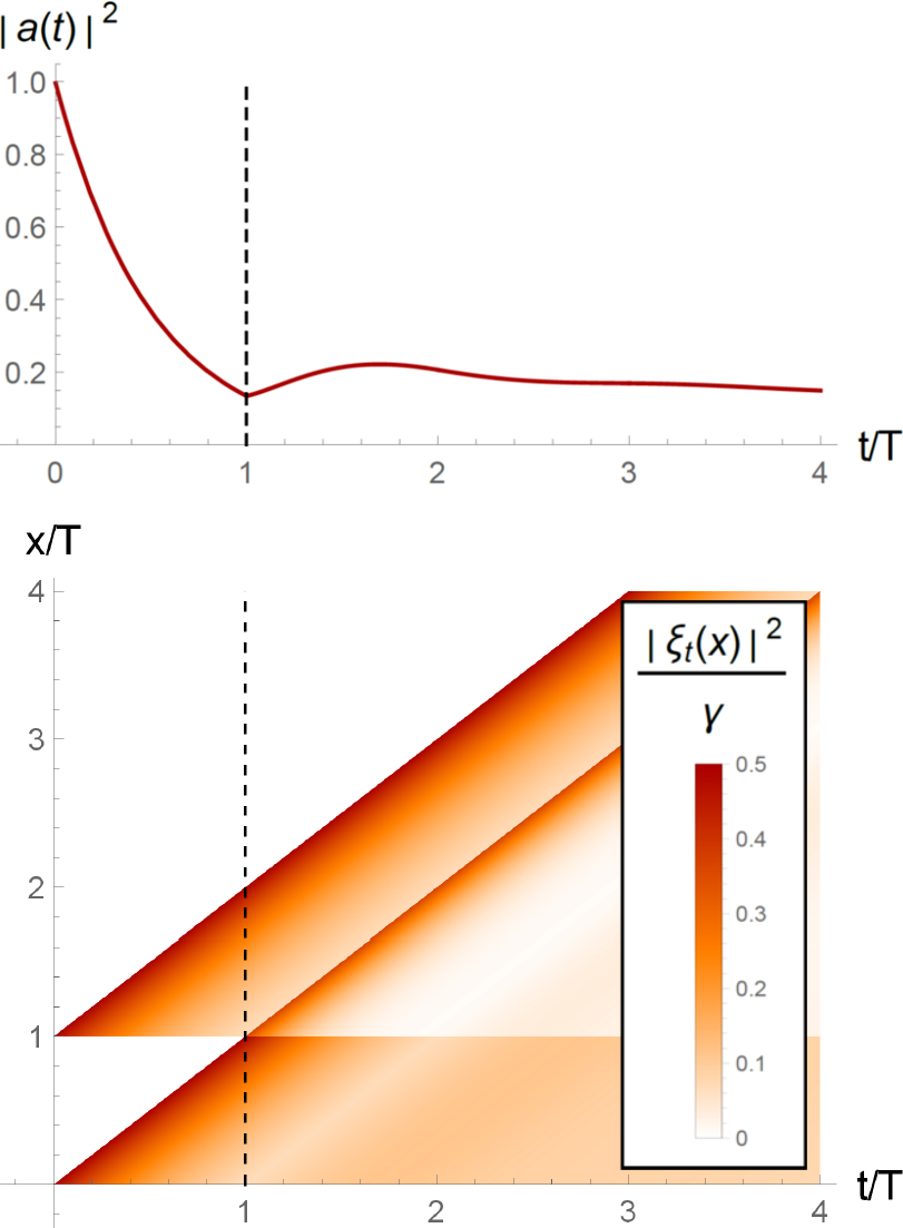
where is as in Eq. (7). We may interpret this new situation as a two-point emission: at time , the qubit emits a photon at both positions , and each of its two spatially separated part propagates separately in the positive direction of the axis up to the time . See Fig. 1(b). Notice that the two components, up to normalisation, are two exact copies of the wavefunction of the one-point emission, and in particular the overall norm is the same as before. In this sense, at times smaller than , this system behaves like the superposition of two identical, independent “copies” of the previous system. When , one of the photon branches starts interfering back with the qubit and this simple picture ceases immediately to hold: is no longer an exponential function, and will no longer satisfy Eq. (10). This is clearly visible in the plots of and in Fig. 1(c).
As a result, the evolution of the qubit state , obtained in the same way as in Eq. (8) will be completely indistinguishable from the previous one, as long as . In fact, the form factor given by Eq. (9) is just one possible example: the same result would be obtained by taking into account any number of spatially separated nonlocal point interactions: until the various components of the photon wavefunction do not propagate to the next point and start interfering. We can thus construct a large family of quantum systems with the HNM property, as shown in Ref. Burgarth et al. 2021b. In all such cases, we obtain non-Markovian processes which, as long as we examine their free dynamics, “look exactly like” a Markovian process at times , despite ultimately starting to show non-Markovian behaviour at .
This argument, however, still does not take into account multitime correlations of the qubit, which are accessible by means of external interventions on the system. The above result only accounts for correlations between two times, and in general, correlations at all orders should be proved to vanish for assessing that a process is Markovian.
We will make a few remarks before going on and examining multitime correlations. The spin-boson model (4)–(5), with a singular point interaction and with boson Hamiltonian the right shift generator, can be mapped into an SLH model Combes et al. 2017; Gregoratti 2001, with , , and . As such, it is associated with an Itô quantum stochastic differential equation Hudson and Parthasarathy 1984, with a regression property for all multitime correlation functions, and thus with a strong quantum Markovianity property Li et al. 2018. In this respect, the model with a two-point interaction (9), is a non-Markovian generalisation of an SLH model, in which a feedback is considered, see Figure 1(b). This is also linked with the theory of time-delayed coherent quantum feedback Grimsmo 2015, where a similar scheme was considered. Interestingly enough, this theoretical model is an effective description of the experimental implementation of superconducting artificial giant atoms in waveguide electrodynamics Kannan et al. 2020.
Multitime correlations in HNM Models.— Now we turn to the main question of this Article, that is, whether higher order correlations are present in HNM models. In other words, can intermediate interventions reveal hidden non-Markovianity already in the time interval ? Such interventions can cause the system to go in higher-excitation sectors, which are not solvable; the “indistiguishability” between this model and the reference one may, in principle, be broken.
However, as shown in the Appendix, the system with form factor (9) satisfies a property which will be crucially employed here: given a time and any wavefunction which satisfies
| (11) |
then the following property holds for in (3):
| (12) |
where is the free evolution of . Physically, Eq. (12) can be interpreted as follows: since wavefunctions satisfying (11) are sufficiently far apart from the point interactions, they freely propagate without interfering. In particular, this implies that, for such that , we have
| (13) |
with being the boson wavefunction (10). This simple equation encodes a fundamental property of the system, which proves to be the key point of our discussion: as long as the total time of observation is less than , the boson field cannot carry information about the non-Markovianity of the system. Local operations of any kind on the qubit cannot modify this simple picture: however we intervene on the qubit via a process as depicted in Fig. 1(b), with all interventions made at times , all photons emitted in the process will evolve exactly as they would in the absence of coupling. Consequently, all multitime correlations vanish, and the process is genuinely Markovian up to a time . Only at later times the field will “recognise” the inherently non-Markovian structure of the coupling.
This argument is fully backed up by a lengthy but straightforward calculation which shows that, as a consequence of property (13), the process tensor for all the HNM models (and, in particular, for the two models discussed in the previous section) is exactly the same, and has the factor form (2), as long as . However, for and , the process tensor will display correlations. Therefore, all HNM models define a quantum process which is genuinely Markovian within a finite time window and (apart from the one-point interaction which is Markovian for all times) genuinely non-Markovian outside that window. The proof is shown in the Appendix for three-time correlations, and may be easily generalised for an arbitrary number of interventions.
What is surprising here is that these intricate memory structures stem from a rather simple time-independent Hamiltonian. This is a feature that may be used to engineer intricate temporal correlations, which we discuss in our concluding remarks.
Conclusions.— When the Markovian properties of quantum noise were first investigated Lindblad 1980; Accardi et al. 1982 the emphasis was on the natural properties of a given system. Nowadays, quantum information adds an important engineering perspective, which asks how systems behave differently in the context of design and control. This means that device characterisation needs to test quantum systems under a wide range of interventions. We have shown here that it is ultimately impossible, in general, to fully conclude if a given system is truly Markovian, no matter how complex this characterisation is. Using such a device under Markovian design assumptions can then lead to unexpected behaviour at a later stage.
On the other hand, open systems quickly become too complex. Simple models like SP, CG, and now HNM, allow us to form simple building block for complex processes and offer keen intuition about the structures of quantum stochastic processes. There are several features of the HNM of interest. Firstly, this is an example of a process which has no short-term memory and only long-term memory. Moreover, this model could serve as the basis for constructing processes with only higher-order correlations, that is, a process where only correlations above four points in time are nonvanishing. Finally, HNM can serve as an Ansatz for simulating processes with slow decaying correlations. To do this, we may add more loops to at the top in Fig. 1(b) and create a self-similar structure that will reduce the correlation strength geometrically after a delay of . The slowly decaying correlation in time here will be akin to the highly common noise. Modelling processes with slowly decaying noise is thought to be hard for the same reasons as the tensor network representation of such correlation is non-trivial Orús 2014.
Acknowledgements.
DB acknowledges funding by the ARC (project numbers FT190100106, DP210101367, CE170100009). PF and DL were partially supported by the Italian National Group of Mathematical Physics (GNFM-INdAM), by Istituto Nazionale di Fisica Nucleare (INFN) through the project “QUANTUM”, and by Regione Puglia and QuantERA ERA-NET Co-fund in Quantum Technologies (GA No. 731473), project PACE-IN. KM is supported through Australian Research Council Future Fellowship FT160100073, Discovery Project DP210100597, and the International Quantum U Tech Accelerator award by the US Air Force Research Laboratory.Appendix A
A.1 Dynamics in the single-excitation sector
As discussed in the main text, the Hamiltonian given by , with as in Eq. (4) and as in Eq. (5), preserves the total number of excitations of states. Let us consider the single-excitation sector, spanned by states in the form
| (14) |
for some and some wavefunction , with being the operator that creates a photon with wavefunction , as defined in Eq. (3).
The restriction of to vectors in the form (14), known as the Friedrichs-Lee Hamiltonian, is exactly solvable; see Refs. Lonigro et al. 2019; Facchi et al. 2021. We will be interested in the evolution of the states and ; the first one is readily shown to evolve trivially, for the second one we need to solve the Schrödinger equation, where we set :
| (15) |
with initial conditions and , with , being respectively the derivatives with respect to and .
While this system has already been solved in Ref. Burgarth et al. 2021b, we will briefly discuss here its resolution since we are now working in the (different, but equivalent) position representation. The second equation with initial condition at can be solved formally with respect to the first one:
| (16) |
In the main text we have considered the following two choices:
- •
;
- •
.
In the first case, Eq. (16) simplifies as follows:
| (17) | |||||
where is the characteristic function of the interval , i.e. for and is zero otherwise. Substituting this expression in the first equation in (15), it can be shown, as discussed extensively in the Appendix of Ref. Burgarth et al. 2021b, that is a pure exponential function:
| (18) |
with being the dressed (renormalised) excitation energy of the qubit. See Refs. Lonigro et al. 2019; Facchi et al. 2021 for a rigorous approach to the renormalisation in the Friedrichs-Lee model. By substituting Eq. (18) into Eq. (17), one obtains
| (19) |
as reported in Eq. (7) in the main text. Notice that
| (20) |
In the second case, Eq. (16) becomes
| (21) | |||||
Notice that is the sum of two identical, compactly supported wavefunctions evaluated at and respectively; in particular, for their supports are disjoint. See also Fig. 1(c) in the main text.
Substituting this expression in the first equation in (15), again can be computed exactly at all times, as discussed in Ref. Burgarth et al. 2021b, while its expression will be involved for , for it is, again, a pure exponential given by Eq. (18), and therefore
| (22) |
again with given by Eq. (7). Notice that, for ,
| (23) | |||||
again as an immediate consequence of the fact that, for , the wavefunction is composed of two identical, disjointly supported terms.
Finally, we remark that the generalisation of these calculations to the case of a form factor
| (24) |
is straightforward: for each admissible choice of the coefficients and the points , the function will again be a pure exponential up to and the resulting single-photon wavefunction will be a superposition of rescaled and translated components ; again, the property will hold.
A.2 Proof of Eq. (12)
We will now show that Eq. (12) holds, respectively in the following cases:
- •
if , whenever is not supported in ;
- •
if , whenever is not supported in ,
the generalisation to a form factor (24) again being immediate.
Let the Heisenberg evolution of ; as such, it must satisfy
| (25) |
On the other hand, the free evolution satisfies
| (26) |
where the free boson Hamiltonian is the second quantisation of . Now, in the case of a point interaction at , we get
| (27) |
Therefore, if for all , i.e. if the boson wavepacket is supported outside the space interval , then for all times we get that
| (28) |
whence , for all , since they satisfy the same differential equation with the same initial condition. In particular, .
In the case of a 2-point interaction we get instead
| (29) |
and the free field evolution equals the Heisenberg evolution as far as for all .
A.3 Choi state with nonlocal point interactions
Let us evaluate the Choi state for a two-times process tensor on the Hamiltonian with form factor given by Eq. (9), at times with , starting from the system and the environment prepared in the global pure state . In particular, we will show that the Choi state is exactly the same that would be obtained with the form factor given by , which corresponds to a Markovian model, and therefore no deviation from Markovianity is detected if the process lasts less than . The computation can be readily generalised for a general -times process, again provided that the final time satisfies .
Following Ref. Milz and Modi 2021, it suffices to consider two couples and of qubits each initially in a maximally entangled state , defined by
| (30) |
First of all, we must compute the state
| (31) |
where is the evolution, for a time , of the subsystem composed by the qubit and the environment (with and the second couple of qubits being uncoupled in the process) and is the evolution, for a time , of the subsystem composed by the qubit and the environment (with and the first couple of qubits being uncoupled in the process). The partial trace of the pure state corresponding to the vector (31) with respect to the environment is the Choi state that we need to compute,
| (32) |
whose components may be arranged in a matrix. Clearly, to compute (31), we must evaluate the following four quantities:
| (33) | |||
| (34) | |||
| (35) | |||
| (36) |
We will report here the calculation of the first term; the remaining ones will follow similarly. First of all, in the time interval the qubit , in the state , interacts with the environment in the state , while all other emitters do not evolve. Recalling the discussion in the first subsection of this Appendix, we have
| (37) |
with as in Eq. (22), and therefore the global state of the system after a time will be given by
| (38) |
and thus
| (39) |
We must finally compute the two states and . The first one is computed exactly as in the previous step:
| (40) |
In order to compute the second state, here we will finally use Eq. (13), which holds as a direct consequence of Eq. (12) provided that , as in our case. We have
We finally obtain
| (41) | |||||
Notice that, in the two-photon state in Eq. (41), the two creation operators commute, since is supported in while is supported in , the supports being disjoint.
The remaining three pieces can be computed similarly:
| (42) | |||||
| (43) | |||||
| (44) |
The pattern is as follows. Only the qubit and may flip, and only the transition is allowed; for each possible combination,
- •
will yield a phase factor , ;
- •
will yield an exponential factor , ;
- •
will yield a boson, i.e. an operator if the transition happens during the second step (a boson propagates starting from up to ), and if it happens in the first step (a boson propagates from time to , and then is rigidly translated for an additional time ).
The sum of the terms in Eqs. (41)–(44) finally gives the vector in (31). Now all matrix elements of the Choi state (32) can be computed: since each of the addends corresponds to a distinct qubit state, we must simply evaluate the norms of all boson components of the states in Eqs. (41)–(44). But recalling that, as long as ,
- •
has exactly the same expression that would be obtained in the reference model with , i.e. ;
- •
the boson wavefunction has exactly the same norm, by Eq. (23), of the boson wavefunction that would be obtained in the reference model, i.e. , and similarly the scalar products between the wavefunctions and are equally zero,
we conclude that, as long as we consider a process tensor lasting less than , the Choi states for the reference model and the one with a nonlocal double interaction are exactly identical. More generally, this holds when taking into account any form factor as in Eq. (24).
Therefore, to prove our claim, it suffices to show explicitly that the reference model is Markovian in the sense of Eq. (2). By a direct computation one has the following expressions for the Choi states of the model: the single-time Choi state is a 4x4 matrix in the form
| (45) |
while the two-times Choi state is a 16x16 matrix that can be written, in a block diagonal structure, as
| (46) |
where
With these expressions, a direct computation shows that the Choi states of the reference model satisfy the Markov property:
| (72) |
This calculation is immediately generalisable to a process tensor with a larger number of steps.
References
- Preskill (2013) J. Preskill, Sufficient condition on noise correlations for scalable quantum computing, Quant. Inf. Comp. 13, 181 (2013).
- Helsen et al. (2020) J. Helsen, I. Roth, E. Onorati, A. H. Werner, and J. Eisert, A general framework for randomized benchmarking (2020), arXiv:2010.07974 [quant-ph] .
- Rivas et al. (2014) Á. Rivas, S. F. Huelga, and M. B. Plenio, Quantum non-Markovianity: characterization, quantification and detection, Rep. Prog. Phys. 77, 094001 (2014).
- Li et al. (2018) L. Li, M. J. Hall, and H. M. Wiseman, Concepts of quantum non-Markovianity: A hierarchy, Phys. Rep. 759, 1 (2018).
- Milz and Modi (2021) S. Milz and K. Modi, Quantum Stochastic Processes and Quantum non-Markovian Phenomena, PRX Quantum 2, 030201 (2021).
- Viola et al. (1999) L. Viola, E. Knill, and S. Lloyd, Dynamical decoupling of open quantum systems, Phys. Rev. Lett. 82, 2417 (1999).
- Arenz et al. (2018) C. Arenz, D. Burgarth, P. Facchi, and R. Hillier, Dynamical decoupling of unbounded hamiltonians, J. Math. Phys. 59, 032203 (2018).
- White et al. (2020) G. A. L. White, C. D. Hill, F. A. Pollock, L. C. L. Hollenberg, and K. Modi, Experimental non-Markovian process characterisation and control on a quantum processor, Nat. Commun. 11, 6301 (2020).
- Lindblad (1980) G. Lindblad, Response of Markovian and non-Markovian quantum stochastic systems to time-dependent forces, (unpublished), Stockholm (1980).
- Accardi et al. (1982) L. Accardi, A. Frigerio, and J. T. Lewis, Quantum stochastic processes, Pub. Res. Inst. Math. Sci. 18, 97 (1982).
- Arenz et al. (2015) C. Arenz, R. Hillier, M. Fraas, and D. Burgarth, Distinguishing decoherence from alternative quantum theories by dynamical decoupling, Phys. Rev. A 92, 022102 (2015).
- Milz et al. (2019) S. Milz, M. S. Kim, F. A. Pollock, and K. Modi, Completely Positive Divisibility Does Not Mean Markovianity, Phys. Rev. Lett. 123, 040401 (2019).
- Taranto et al. (2019) P. Taranto, F. A. Pollock, and K. Modi, Memory Strength and Recoverability of Non-Markovian Quantum Stochastic Processes, arXiv:1907.12583 (2019).
- Burgarth et al. (2020) D. Burgarth, P. Facchi, and R. Hillier, Control of quantum noise: on the role of dilations, arXiv:2010.00279 (2020).
- Gregoratti (2001) M. Gregoratti, The Hamiltonian Operator Associated with Some Quantum Stochastic Evolutions, Commun. Math. Phys. 222, 181 (2001).
- Burgarth et al. (2021a) D. Burgarth, P. Facchi, M. Fraas, and R. Hillier, Non-Markovian noise that cannot be dynamically decoupled by periodic spin echo pulses, SciPost Phys. 11, 27 (2021a).
- Burgarth et al. (2021b) D. Burgarth, P. Facchi, M. Ligabò, and D. Lonigro, Hidden non-Markovianity in open quantum systems, Phys. Rev. A 103, 012203 (2021b).
- Wolf et al. (2008) M. M. Wolf, J. Eisert, T. S. Cubitt, and J. I. Cirac, Assessing non-Markovian quantum dynamics, Phys. Rev. Lett. 101, 150402 (2008).
- Guarnieri et al. (2014) G. Guarnieri, A. Smirne, and B. Vacchini, Quantum regression theorem and non-Markovianity of quantum dynamics, Phys. Rev. A 90, 022110 (2014).
- Pollock et al. (2018a) F. A. Pollock, C. Rodr\́mathrm{i}guez-Rosario, T. Frauenheim, M. Paternostro, and K. Modi, Non-Markovian quantum processes: Complete framework and efficient characterization, Phys. Rev. A 97, 012127 (2018a).
- Pollock et al. (2018b) F. A. Pollock, C. Rodr\́mathrm{i}guez-Rosario, T. Frauenheim, M. Paternostro, and K. Modi, Operational Markov Condition for Quantum Processes, Phys. Rev. Lett. 120, 040405 (2018b).
- Costa and Shrapnel (2016) F. Costa and S. Shrapnel, Quantum causal modelling, New J. Phys. 18, 063032 (2016).
- van Kampen (1998) N. G. van Kampen, Remarks on non-Markov processes, Braz. J. Phys. 28, 90 (1998).
- Davies and Lewis (1970) E. Davies and J. Lewis, An operational approach to quantum probability, Commun. Math. Phys. 17, 239 (1970).
- Chiribella et al. (2009) G. Chiribella, G. M. D’Ariano, and P. Perinotti, Theoretical framework for quantum networks, Phys. Rev. A 80, 022339 (2009).
- Milz et al. (2020a) S. Milz, F. Sakuldee, F. A. Pollock, and K. Modi, Kolmogorov extension theorem for (quantum) causal modelling and general probabilistic theories, Quantum 4, 255 (2020a).
- Strasberg and D\́mathrm{i}az (2019) P. Strasberg and M. G. D\́mathrm{i}az, Classical quantum stochastic processes, Phys. Rev. A 100, 022120 (2019).
- Milz et al. (2020b) S. Milz, D. Egloff, P. Taranto, T. Theurer, M. B. Plenio, A. Smirne, and S. F. Huelga, When Is a Non-Markovian Quantum Process Classical?, Phys. Rev. X 10, 041049 (2020b).
- White et al. (2021a) G. A. L. White, F. A. Pollock, L. C. L. Hollenberg, C. D. Hill, and K. Modi, Non-Markovian Quantum Process Tomography, arXiv:2106.11722 (2021a).
- Giarmatzi and Costa (2021) C. Giarmatzi and F. Costa, Witnessing quantum memory in non-Markovian processes, Quantum 5, 440 (2021).
- Milz et al. (2021) S. Milz, C. Spee, Z.-P. Xu, F. A. Pollock, K. Modi, and O. Gühne, Genuine Multipartite Entanglement in Time, SciPost Phys. 10, 141 (2021).
- White et al. (2021b) G. A. L. White, F. A. Pollock, L. C. L. Hollenberg, C. D. Hill, and K. Modi, Diagnosing temporal quantum correlations with compressed non-Markovian calipers, arXiv:2107.13934 (2021b).
- (33) Strictly speaking, the sum of (4) and (5) is a well-defined (and self-adjoint) Hamiltonian only when is square integrable, which is clearly not the case here; however, as discussed in Lonigro et al. 2019; Facchi et al. 2021, via a renormalisation procedure (singular coupling limit) a self-adjoint operator can be obtained even in the cases that we are considering.
- Fang et al. (2018) Y.-L. L. Fang, F. Ciccarello, and H. U. Baranger, Non-Markovian dynamics of a qubit due to single-photon scattering in a waveguide, New J. Phys. 20, 043035 (2018).
- Combes et al. (2017) J. Combes, J. Kerckhoff, and M. Sarovar, The SLH framework for modeling quantum input-output networks, Adv. Phys.: X 2, 784 (2017).
- Hudson and Parthasarathy (1984) R. L. Hudson and K. R. Parthasarathy, Quantum Ito’s formula and stochastic evolutions, Commun. Math. Phys. 93, 301 (1984).
- Grimsmo (2015) A. L. Grimsmo, Time-delayed quantum feedback control, Phys. Rev. Lett. 115, 060402 (2015).
- Kannan et al. (2020) B. Kannan, M. J. Ruckriegel, D. L. Campbell, A. Frisk Kockum, J. Braumüller, D. K. Kim, M. Kjaergaard, P. Krantz, A. Melville, B. M. Niedzielski, A. Vepsäläinen, R. Winik, J. L. Yoder, F. Nori, T. P. Orlando, S. Gustavsson, and W. D. Oliver, Waveguide quantum electrodynamics with superconducting artificial giant atoms, Nature 583, 775 (2020).
- Orús (2014) R. Orús, A practical introduction to tensor networks: Matrix product states and projected entangled pair states, Ann. Phys. 349, 117 (2014).
- Lonigro et al. (2019) D. Lonigro, P. Facchi, and M. Ligabò, The Friedrichs-Lee Model and its Singular Coupling Limit, Proceedings 12, 17 (2019).
- Facchi et al. (2021) P. Facchi, M. Ligabò, and D. Lonigro, Spectral properties of the singular Friedrichs-Lee Hamiltonian, J. Math. Phys. 62, 032102 (2021).