On the Quality of Uncertainty Estimates from Neural Network Potential Ensembles
Abstract
Neural network potentials (NNPs) combine the computational efficiency of classical interatomic potentials with the high accuracy and flexibility of the ab initio methods used to create the training set, but can also result in unphysical predictions when employed outside their training set distribution. Estimating the epistemic uncertainty of a NNP is required in active learning or on-the-fly generation of potentials. Inspired from their use in other machine-learning applications, NNP ensembles have been used for uncertainty prediction in several studies, with the caveat that ensembles do not provide a rigorous Bayesian estimate of the uncertainty. To test whether NNP ensembles provide accurate uncertainty estimates, we train such ensembles in four different case studies, and compare the predicted uncertainty with the errors on out-of-distribution validation sets. Our results indicate that NNP ensembles are often overconfident, underestimating the uncertainty of the model, and require to be calibrated for each system and architecture. We also provide evidence that Bayesian NNPs, obtained by sampling the posterior distribution of the model parameters using Monte-Carlo techniques, can provide better uncertainty estimates.
I Introduction
Interatomic potentials (IPs) are a long-established method to describe the potential energy and forces in atomic systems, and have provided important insights into the physics of atomic structures in the last seven decades Alder et al. 1955; Rahman 1964; Ercolessi and Adams 1994; González 2011. A notable advantage of IPs over first-principles approaches such as density functional theory (DFT) Hohenberg and Kohn 1964; Kohn and Sham 1965 and first-principles molecular dynamics Car and Parrinello 1985 is their higher computational efficiency, allowing the simulation of larger systems over longer time scales. In recent years, machine-learning techniques have been successfully applied to develop force fields for atomistic simulations Ceriotti 2019; Musil et al. 2021; Behler 2021. Among other machine-learning techniques, (deep) neural networks (NN) can be used as force and energy predictors, resulting in neural network potentials (NNPs), which have led to significant advances in atomistic simulation, combining high computational efficiency with great flexibility and accuracy Zuo et al. 2020; Li et al. 2020; Qi et al. 2021. One assumption behind IPs is that the energy of the system can be described as a sum over atomic energies: . Another assumption behind most NNPs is that the atomic energy is a function of the local neighborhood of that specific atom, that is all atoms within a radial cutoff distance, . Any IP, and therefore also NNP, should be invariant to translation, rotation, and permutation of atoms in the system. This is most commonly achieved by constructing a descriptor of the atomic environment that displays those symmetries.
One approach to generate NNPs is to use NNs to learn parameters of a physics-inspired functional form, for example to tackle long-range electrostatic contributions to energy and forces Ghasemi et al. 2015; Bleiziffer et al. 2018; Nebgen et al. 2018; Deng et al. 2019, which should be relevant in ionic systems. However, recent work has shown that NNPs are capable of accurate predictions in ionic systems without explicitly including long-range interactions Marcolongo et al. 2020; Huang et al. 2021. NNPs can also be used directly for prediction of energies, forces, and stresses, without enforcing a particular functional form. As a first example, Behler and Parrinello implemented a NNP Behler and Parrinello 2007 using atomic symmetry functions as an SO(3) invariant descriptor. Another example is DeePMD developed by Zhang et al., where the relevant descriptors are learned during the training and SO(3) invariance is encoded in the mathematical form of the first layers Zhang et al. 2018a.
Convolutional neural networks and graph convolutional neural networks achieve invariance via the application of tailored convolution filters Duvenaud et al. 2015; Hy et al. 2018; Ryczko et al. 2018; Xie and Grossman 2018; Klicpera et al. 2020, one prominent example being Schnet Schütt et al. 2017; Schütt et al. 2018. A recent addition to the plethora of neural network potentials are tensor-field NNPs, which encode SO(3) equivariance in the convolutional operations Thomas et al. 2018; Mailoa et al. 2019. Batzner et al. released NequIP Batzner et al. 2021, an efficient implementation of a NNP using equivariant convolutions.
While the architecture of the network and the type and size of the input descriptor are of great importance to build an accurate NNP, training the model with an extensive data set of high quality is just as relevant. One common approach is to sample configurations with ab initio methods, such as Born-Oppenheimer molecular dynamics at different thermodynamic conditions Zhang et al. 2018b; Zuo et al. 2020. Another possibility is an active-learning approach, a repeated cycle of exploration, labeling, and (re)training of a model as follows:
- 1.
exploring configurations space, e.g., via molecular dynamics, using a NNP obtained in the previous iteration or from an initial training.
- 2.
labeling a subset of configurations using an ab initio method.
- 3.
training a new NNP with the labeled configurations.
As a first example, Marcolongo et al. Marcolongo et al. 2020 trained a NNP in this iterative fashion to model Li-ion diffusion in solid-state electrolytes, where the configurations in the second step were selected randomly from the molecular-dynamics trajectory of the first step, and were therefore sampled according to the Boltzmann distribution. A possible disadvantage of this method is that data selected randomly could be redundant, adding no new information to the training set. Several works in the past have concentrated on detecting configurations that provide additional data that are not already covered by the training set. Li et al. 2015; Miwa and Ohno 2017. This can either enable active exploration of configuration space to obtain better coverage, or so-called on-the-fly training during a molecular-dynamics or Monte-Carlo trajectory, proposed as early as 1997 by Vita and Car Vita and Car 1997 and used or developed further in subsequent work Csányi 2004. Using NNPs in such a scenario can be challenging, as it is very hard to predict when a model is outside the training set distribution Zhang et al. 2019; Wen and Tadmor 2020; Schran et al. 2020. Neural networks are often described as “universal function approximators”. That flexibility directly results in the difficulty to control prediction trends when departing from the training set distribution.
Detecting configurations that provide additional data translates to detecting atomic environments of high epistemic uncertainty. While aleatoric uncertainty is due to noise inherent in the labels, epistemic uncertainty is due to lack of data and is the subject of this work Kendall and Gal 2017; Tagasovska and Lopez-Paz 2019; Abdar et al. 2021. In the remainder, we simply refer to uncertainty, meaning epistemic uncertainty originating from data scarcity. One approach to estimate the uncertainty of the prediction of neural networks relies on the prediction of several instances, so-called neural-network ensembles, where the uncertainty is estimated from the deviation of the output of different models that were trained on the same data. The members of the ensemble ideally have different architectures or, as a minimal criterion, have the same architecture but are initialized independently. Ensemble networks led to promising results in many machine-learning applications Lakshminarayanan et al. 2017; Pearce et al. 2020; Yao et al. 2019. Ensemble NNPs were, for example, used by Zhang et al. Zhang et al. 2019, but also other work has relied on similar approaches to select configurations of high model uncertainty Chen et al. 2020; Miwa and Ohno 2017; Jeong et al. 2020. However, the uncertainty derived from ensembles is not, strictly speaking, a Bayesian uncertainty estimate Yarin Gal 2016; Pearce et al. 2020; D’Angelo and Fortuin 2021. The same applies to dropout techniques, which have also been used to estimate uncertainty in NNPs Wen and Tadmor 2020. The method relying on the least approximations to obtain uncertainty estimates are Bayesian NNs MacKay 1992; Neal 1996; Martin et al. 2020, obtained by sampling the posterior distribution of NN parameters. Bayesian NNPs, which do not rely on ensembles or dropout, have not yet been developed to the best of our knowledge, most likely due to the increased complexity and high computational cost of exploring the posterior distribution of the NNP parameters using expensive sampling techniques such as Hamiltonian Monte Carlo Neal 1993; Chandra et al. 2019; Baldock and Marzari 2019; Yao et al. 2019.
In this work, we explore the relationship between the uncertainty predicted by NNP ensembles and the true error of the prediction, showing that ensembles are prone to common bias and overconfident predictions, depending on model architecture and the system, requiring careful calibration of the uncertainty. Furthermore, we compare choosing configurations based on the predicted uncertainty, as proposed by Zhang et al. Zhang et al. 2019, to random sampling during exploration, as done by Marcolongo et al. Marcolongo et al. 2020. In Sec. II we explain the methods used in this work. The results are shown and discussed in Sec. III and we present our conclusion in Sec. IV.
II Methods
II.1 Systems and NNPs
In order to allow for general conclusions, we used training and validation data from four very different atomic systems: an atomic dimer, an aluminum surface slab, bulk liquid water, and a benzene molecule in vacuum. The training and validation data were produced with a Lennard-Jones potential, density-functional theory, or the highly accurate coupled-cluster single-, double-, and perturbative triple-excitations method, CCSD(T). The neural-network architectures we tested were a custom-built neural network, the DeePMD Zhang et al. 2018a framework, and the NequIP Batzner et al. 2021 potential.
As a first case study, we trained a NNP on the potential energy surface (PES) of an atomic dimer, i.e., two atoms of the same species in vacuum. For this purpose, we chose a parametrized model as the ground truth, namely the Lennard-Jones IP, where the energy is a function of the interatomic distance :
| (1) |
where we set and nm (which are the parameters used by Rahman Rahman 1964 to study atomic correlation in liquid argon). In the range of interest (0.3 to 0.7 nm) we chose randomly ten training points according the Boltzmann weight with K. Such a simple system allows for a significant reduction of the dimensionality of the problem and for a custom-built NNP, leading to better interpretability of the results.
We implemented a custom NNP using the pytorch framework, with an input size of one (the interatomic distance), a hidden layer of 64 neurons, and an output layer of one (the energy). A neural network requires a non-linear activation function, and common choices of such activation functions are the hyperbolic tangent tanh, the sigmoid function, rectified linear units (ReLU), continuously differentiable exponential linear units (CELU) Barron 2017, and Gaussian error linear units (GELU). These activation functions are shown in Fig. S1 of the SI. We implemented NNPs with each type of activation function, as well as one NNP where the activation function of each neuron was randomly chosen among aforementioned functions. We trained each NNP with the Adam optimizer for 50’000 steps with a learning rate of .
We used the smooth edition of DeePMD Zhang et al. 2018a, as implemented in the deepmd-kit package (version 1.3.3), to build a potential for bulk and surface aluminum (Al) and for liquid water. The DeePMD NNPs had three layers for the local-embedding network, their sizes being 32, 64, and 128, respectively, and three layers for the fitting network, each consisting of 256 neurons. The training was performed using stochastic-gradient descent with an exponentially declining learning rate.
To have a more realistic and complex scenario than the atomic dimer, we trained the DeePMD potential on forces and energies from an Al(100) surface with an adatom of the same species. The bulk portion of the system is representative of metals, while the presence of the surface leads to additional complexity. Extensive FPMD simulations of this system were performed by Nguyen et al. of a system of 295 atoms Nguyen et al. 2018, consisting of six layers of Al (49 atoms per layer) with an additional atom on the surface. The calculations were performed with Born-Oppenheimer molecular dynamics as implemented in the Quantum ESPRESSO (QE) distribution Giannozzi et al. 2009 using the Perdew-Burke-Ernzerhof (PBE) exchange-correlation functional Perdew et al. 1996 in the canonical (NVT) ensemble. The temperatures investigated were 300 – 600 K in steps of 100 K, and additionally 800 and 1000 K, with 30 ps of dynamics collected for every simulation. We selected evenly distributed snapshots from each trajectory: 144 snapshots from the trajectory at 1000 K, 72 snapshots at 800 K, and 36 snapshots from the simulations at 300 – 600 K. For each temperature, 12 snapshots were retained for validation in order to obtain a temperature-dependant validation error. We used the remaining snapshots (training set) to train a NNP using DeePMD Zhang et al. 2018a, with the parameters given in Fig. S2 of the SI. An additional 91 snapshots were created from an exploration with the NNP at 1000 K and added to the training set. Training the DeePMD NNP with this data set, we obtained a trained model . One hundred additional snapshots were sampled by exploring with the same system at 1500 K in order to obtain an additional validation set, .
We also trained a NNP with DeePMD for the commonly studied system of bulk water, representative of highly ergodic liquid systems with high directionality of bonds, resulting in the complex chemistry of water. We used the data set created by Cheng et al. Cheng et al. 2018; Cheng et al. 2019 of 64 water molecules in a cubic periodic cell. We split the data set into four equally large data sets of 300 configurations each according to the potential energy of the configuration, where the potential energy of a configuration in set is smaller than (or equal to) the energies of configuration in set :
| (2) |
The energy distribution of the four sets of configurations is shown in Fig. S8 of the SI. The model was trained with and were kept as validation sets. The parameters employed for DeePMD (Al and water) are given in Fig. S2 of the SI.
Last, we employed NequIP, developed by Batzner et al. Batzner et al. 2021, to fit a potential for the benzene molecule in vacuum, which is a good representative of covalently bonded systems. Our NequIP NNP had three convolution layers, and eight was the dimension of the hidden layer and the number of features. We used a data set of 1500 configurations of C6H6, produced by Chmiela et al. Chmiela et al. 2018, who sampled configurations using MD in the canonical (NVT) ensemble at 500 K, and re-calculated forces and energies using CCSD(T) for this data set. We ordered the set of 1500 configurations by potential energy and split the data into six batches of equal size, obtaining independent sets of 250 configurations each. The energy distribution of the six sets of configurations is shown in Fig. S9 of the SI. Also in this case, the potential energy of a configuration in set is smaller (or equal) to the energies of configuration in set :
| (3) |
As in the case study of liquid water, we trained the NNP on the set of lowest-energy configurations (), and used as validation sets. The Adam optimizer was used for the training, with a learning rate of 0.01, and the training was stopped after 500 epochs (complete passes over the training data). All parameters are reported in Fig. S3 of the SI.
II.2 NNP ensembles
Unless stated differently, we trained NNPs with the same data to estimate the ensemble uncertainty, which we found to be converged at that ensemble size. These models were initialized independently via the input of different seeds, which affected both the parameter initialization and the order of sample selection during stochastic gradient descent, where applicable. From the ensemble of NNPs, we computed the mean prediction and the standard deviation for every force component :
| (4) | ||||
| (5) |
where the subscripts and give atomic indices and spatial dimensions, respectively, and iterates over models of the ensemble. is the predicted model uncertainty of the force in direction of atom .
The error of the model was calculated (on a validation/test set) from the difference of the predicted (mean) force and the ab initio force (the label):
| (6) |
II.3 Bayesian NNP
The simplicity of the NNP for the atomic dimer and the small amount of training data (ten one-dimensional training points) allowed for a Bayesian estimate of the posterior probability of the weights , given the data :
| (7) |
where is the likelihood of the data, is the prior, and the marginal likelihood. The likelihood of the data given the parameters of a function , assuming Gaussian white noise of variance in the observations, is given by
| (8) |
where is the mean-squared error loss function and the number of samples.
The prior of the parameters, , was set to the normal distribution with , which we evaluated via a curvature criterion. We ignored , the marginal likelihood, since it is independent of . Inserting Eq. (8) and the Gaussian prior into Eq. (7), we obtain an energy or cost function of the parameters of the network that can be sampled at a fictitious temperature MacKay 1992; Chandra et al. 2019; Baldock and Marzari 2019; Wenzel et al. 2020:
| (9) |
We sampled this landscape using Hamiltonian Monte Carlo (HMC) Neal 2011, with the Hamiltonian dynamics being integrated with the velocity Verlet integrator Verlet 1967. We set the fictitious temperature to 0.05 (resulting in a cold posterior Wenzel et al. 2020) and used 10’000 steps of Hamiltonian dynamics, with a timestep of 0.015, which resulted in an acceptance rate of 0.675 of Monte-Carlo moves, close to the optimal acceptance rate of 0.65 Neal 2011. We sampled the parameter distribution by selecting 100 models from the MC trajectory to calculate mean and uncertainty as for the NNP ensembles.
II.4 Statistical analysis
We interpret the ensemble uncertainty as a predictor for the error . A straightforward approach, also employed by Zhang et al. Zhang et al. 2020, is to classify configurations based on an uncertainty threshold . Configurations with all were classified as low error- and were classified as high-error configurations otherwise. The condition was given by . We note that and did not have to be equal, in order to account for systematic underestimates. We formulated two distinct requirements for the uncertainty:
- 1.
A requirement for accurate results is that configurations that produce a high error , due to lack of training data in that region of configuration space are detected via a high uncertainty, .
- 2.
A computational requirement is to achieve high precision for high-error configurations, in order to avoid falsely selecting many configurations that are described well by the model.
The first requirement is given by the true positive rate (TPR), also called recall or sensitivity, which is given by the ratio of correctly positive prediction among all elements with the following condition:
| (10) |
where TP and FN refer to true positives ( and ) and false negatives ( and ), respectively. The second requirement, stating that we want to maximize the ratio of true high-error configuration to high-uncertainty configurations, is described by another metric, the precision or positive predictive value (PPV):
| (11) |
where refers to the false positives ( and ).
III Results and discussion
III.1 The atomic dimer


The custom NNP for the atomic dimer receives a scalar input (the distance), and predicts the energy, and has 64 hidden units. The predictions of this model using the hyperbolic tangent (tanh) as the non-linear activation function are shown for the range of from 0.33 to 0.68 nm in Fig. 1. The NNP ensemble mean is very accurate at predicting the PES in the region of training data, which we call the interpolation regime. In the extrapolation regime, where nm or nm, no data are supplied and the models deviate from the ground truth (blue dash-dotted lines). However, the members of the ensemble deviate in a very similar fashion, most probably due to common biases. This is not only the case when using this particular activation function: all activation functions (ReLU, CELU Barron 2017, GELU, and sigmoid) show the same behavior (see Fig. S4 of the SI). However, different activation functions result in different biases in the region of larger distances ( nm). Using tanh or sigmoid as activation functions leads to underestimates of the energy at nm, whereas other activation functions (ReLU, CELU) lead to overestimates. We suspect that this behavior is because the networks with the latter activation functions are prone to extrapolate the slope from the closest training points. Using the uncertainty of the ensemble as a predictor for low accuracy Zhang et al. 2019 would result in this case study in false positives in data-scarce regions due to the bias in the model.
The NNP ensemble where every neuron within the hidden layer is randomly assigned one out of the different activation functions we study (tanh, sigmoid, GELU, ReLU, and CELU) produces predictions that are more diverse (see Fig. 2) outside the training set distribution. The ensemble displays higher variance of the output in the extrapolative region of nm, which we interpret as evidence that bias has been reduced. The region of smaller distances ( nm) is biased towards slopes of smaller magnitude. Compared to the results of the ensembles with the same architecture, diversifying the NNP ensemble results in lower bias, which is also discussed by Jeong et al. Jeong et al. 2020. The uncertainty of ensembles with a varying model architecture is a better predictor for the accuracy of the model when predicting unseen data and could be useful in active learning. Current approaches employing NNP ensembles Zhang et al. 2019; Chen et al. 2020 do not use varying architectures of the ensemble members to reduce the collective bias. The results of this simple case study of the atomic dimer indicate that this could help in improving the uncertainty estimate.
As a last example, we estimated the posterior distribution of the weights using HMC. The Bayesian model predicts (see Fig. 3) a high uncertainty in the extrapolation regime, for both and , and also an increased uncertainty in the region around nm due to lower data density. The Bayesian model compares well to ensembles with the same and with varying architecture, as the bias is further reduced. The uncertainty predicted by the Bayesian NNP resembles most closely our expectation due to the sharp increase of the uncertainty when extrapolating, and a moderate increase in uncertainty when interpolating in regions of low training data density.
III.2 Al(100) surface

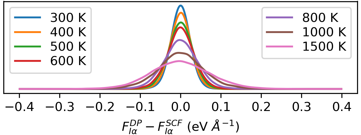


The ensemble of eight DeePMD models, trained on energies and forces of atoms in and on an Al surface, results in an accurate NNP within and close to the training set distribution. The forces on Al atoms for the configurations of three validation sets (, , and ) are plotted in Fig. 4, showing excellent agreement, evidence that the ensemble is able to capture the interatomic interactions of Al in the bulk and on the surface. We observe that the validation sets sampled at higher temperatures lead to higher forces and higher root mean square errors (RMSE) in the prediction, which is expected because the system explores a larger region of phase space at higher temperatures, which translates to a more complex training problem. A histogram of the error for each temperature we studied is shown in Fig. 5, confirming this behavior. The validation set sampled at 1500 K has the highest error. We remind the reader that no configurations sampled at that temperature were used in training, and we mark these as out-of-distribution (ood) samples.
One question of interest is how to detect these ood samples, or – more generally – high-error configurations. The relationship between predicted uncertainty and true error is shown for three validation sets (, , and ) in Fig. 6. We observe that the error is generally about 1 order of magnitude higher than the predicted uncertainty .
No perfect correlation between and is expected, and such a correlation is not a necessary criterion to select snapshots with unacceptable error. A more pragmatic criterion is that a positive constant can be found such that for all (or a significant fraction of) . Such a constant or slope, for example, is visible in Fig. 2(e) of Ref. Vandermause et al. 2020, where the error estimate is given by a Gaussian process regression model. We draw such a line as a guide to the eye in Fig. 6, choosing the line of smallest slope above the data points (and going through the origin). The slope of this line is 62, which means that in order to achieve a very high degree of certainty that the error is below a given threshold , the uncertainty threshold has to be almost 2 orders of magnitude above . We also draw the line that lies above 90% of the data points, resulting in a slope of 14. This shows that even if one is willing to accept a significant amount of high-error configurations, the uncertainty threshold nevertheless lies an order of magnitude above the error threshold. A reliability diagram is shown in the top panel of Fig. 6, where we bin the data points by their uncertainty and plot the mean error for every bin. The mean error increases when the uncertainty is higher, but there are strong signs of miscalibration. A well-calibrated model would result in a reliability diagram close to an identity function.
Similar to previous work Schran et al. 2020; Zhang et al. 2020, we assume that a maximum true error, , exists above which the properties sampled by the dynamics are no longer trustworthy, requiring a need to recalculate this point during active exploration or marking it for labeling. We classify force components of the validation set set according to the true error and try to predict this class using . The TPR, introduced in Eq. (10), is shown in the left panel of Fig. 7. For low (below 10 meV ), it is possible to guarantee that the true error is bounded by a wide range of . In general, the region of high recall or TPR is at the top left of the heat map, towards high and low . The region of high computational efficiency is given by a high precision or PPV and is concentrated in the bottom right, towards high and low . The only region of high precision or PPV and high recall or TPR is in the bottom left, however, this is the region where and are so low that almost all data points are true positives (see Fig. S5 of the SI). In summary, only by giving very strict criteria on the predicted uncertainty is it guaranteed that the true error is bound, which implies that we can only exclude a negligible amount of the data set as low-error points. In an on-the-fly training scenario, where the low error of force components is important, the number of useful calculations will be very low due to the high number of false positives and the low number of true positives (see Fig. S5 of the SI).
In an active-learning scenario, finding all high-error points is not necessary as long as a sufficient number of high-error configurations are discovered to enrich the training set with data, allowing us to relax a very strict threshold . In such a scenario, it is important to find training points for the next iteration that are more likely to be outside the previous training set than if sampled randomly. In Fig. 8 we plot histograms of the true error in the force components when screening for all predictions above ( therefore includes all force components). We observe a shift of the histogram towards larger true errors when selecting for components with higher uncertainties; however, this shift is marginal. This confirms our interpretation of the right panel of Fig. 7, that it is not possible to achieve a high PPV except when declaring almost all data points as high-error points via a very low threshold .
To summarize, we note that ensemble uncertainties are about 1 order of magnitude lower than the errors. This observation needs to be accounted for when relying on ensemble uncertainties. When specifying the error threshold , one needs to investigate which uncertainty criterion this requires. As this case study shows, it is possible that needs to be significantly larger than . Furthermore, the results of this case study indicate that sampling based on an uncertainty criterion Zhang et al. 2019 or sampling randomly Marcolongo et al. 2020 should result in very similar distributions. Random sampling is, for obvious reasons, easier to implement and computationally more efficient and would therefore be preferable.
III.3 Water


In Fig. 9 we show the forces predicted by the DeePMD NNP ensemble against the labels for the three validation sets of bulk water. We note that the training and validation configurations do not originate solely from a molecular-dynamics trajectory, but also from different sampling strategies that lead to significantly higher forces Cheng et al. 2019 than in the previous case study. The error in the forces increases slightly for snapshots of higher potential energies, and the highest RMSE is found for . Nevertheless, the good reproduction of forces in unseen data gives evidence of a very accurate NNP within and close to the training set distribution, gently reducing in accuracy as one moves away from the training examples.
The predicted uncertainty against the true error for all validation sets, plotted in Fig. 10, displays a behavior similar to that in the case study of Al (cf. Fig. 6). The first similarity is that the uncertainty predicted by the NNP ensemble is underestimated with respect to the error by the mean prediction, also by approximately 1 order of magnitude. A distinction, however, is that there is no line of finite slope that bounds all data points from above (i.e., it is not possible to bound the error rigorously), due to the presence of configurations that have been predicted with zero uncertainty but display finite true errors. A line that lies above 90% of the validation points has a slope of 7.7, which is a bit lower than in the previous case study. Nevertheless, the conclusion is the same as for Al(100): the uncertainty threshold needs to be an order of magnitude higher than the error one is willing to accept. Another similarity is the presence of false positives, i.e., force components are predicted relatively accurately despite the high uncertainty associated with that prediction. The reliability diagram in the top panel of Fig. 10 bears closer resemblance to an identity than in the case of Al (cf. Fig. 6). We speculate that this is because the validation set of liquid water is described worse by the ensemble than the validation set of Al(100) (). The fact that the more accurate a model is, the more likely the model is to be overconfident, has also been observed in other work and is believed to constitute a general trend Guo et al. 2017.
As is the case for Al(100), also in liquid water we find regions of high TPR for high errors threshold and low uncertainty bounds , meaning that a strict uncertainty bound is almost guaranteed to find all examples of high true error (see Fig. 11). However, regions of high TPR are also regions of low PPV, implying that the computational efficiency in that regime is low. As a result, there is no region with a F1 score close to 1 (see Fig. S6 of the SI), except for the regime of very strict bounds on uncertainty and error.
In Fig. 12, we plot histograms of the true error distributions for subsets of the validation sets with a minimal (top panel) or maximal (bottom panel) uncertainty. Comparing to the case study of Al (cf. Fig. 8), the histograms change more significantly with increased threshold, meaning that one is likelier to select high-error configurations by using an uncertainty criterion (compared to random selection), which confirms the findings above. The histogram is still peaked at low true errors, but the difference in the histograms gives evidence that the uncertainty criterion can improve the selection of configurations for labeling and retraining in an active-learning scenario.
In this case study, sampling based on the ensemble uncertainty is shown to be advantageous, compared to random sampling, as the probability of including high-error configurations is increased. This has to be weighted against the higher computational cost and complexity of the former approach. Our results for water do not indicate that the true error can be bounded by a limit on the ensemble uncertainty, merely that the probability of picking a high-error configuration is higher if selecting configurations with high ensemble uncertainty, compared to random choice. As in the previous case study, to rely on the ensemble uncertainty would require calibration, as the predicted model uncertainties are of a magnitude significantly lower than that of the model errors.
III.4 Benzene


As a last case study we show the results of the NequIP NNP ensemble trained on the benzene data set. NequIP generalizes well for this training set and can be trained with a comparatively small number of training points. The forces estimated by the NNP ensemble trained on the 250 configurations lowest in potential energy are plotted against the CCSD(T) predictions in Fig. 13 for all validation sets. The RMSE increases for validation sets of higher potential energy, as in the previous example (cf. subsection III.3). The lower complexity of the benzene molecule, compared to water or Al, has allowed us to study which configurations result in comparatively larger model errors. Based on a simple descriptor of the atomic environment, we find that atoms in the training set whose descriptor falls outside the convex hull of training-set descriptors can have higher errors (see Fig. S10 of the SI).
The uncertainty estimates given by the ensemble deviation are plotted against the error in Fig. 14. Here, as for the Al case study (see subsection III.2), it is possible to heuristically bound the error by a line of slope 8.2, which is significantly smaller than a slope of 62 in the case of Al(100), evidence for a lower degree of overconfidence of the ensemble. The line that lies above 90% of the validation points has a slope of 1.4, close to unity. Therefore, unlike the previous examples, the true error and predicted uncertainties are of the same order of magnitude, which means that this system and ensemble are better calibrated. Furthermore, the reliability diagram in the top panel of Fig. 14 resembles the identity function more closely than in the case of Al(100) (cf. Fig. 6), especially if we exclude the right portion of the histogram where the data points are significantly less. We observe that, unlike for liquid water and Al(100), the NequIP ensemble is not overconfident: predictions of an uncertainty have a mean error that is of the same order. Nevertheless, Fig. 15 implies that the same problem persists as for the uncertainty estimates in Al(100) and liquid water, namely that it is not possible to separate efficiently configurations (or force components) of high uncertainty without also including a large amount of false negatives (configurations that are accurately described, but where the ensemble estimates a high uncertainty). In Fig. 16, we show the histograms of the error distribution for subsets of the validation set , screened by the ensemble uncertainty. As for the case of liquid water, the histogram is shifted towards higher-error configurations when excluding low-uncertainty configurations from the validation set. Nevertheless, the histogram remains with its maximum value at low-error configurations, which means that many false positives are included, and the histograms are not significantly different from a random selection. Also in this case study, there is evidence to suggest that sampling based on the uncertainty Zhang et al. 2019 can result in an improved training set with a higher likelihood of unseen new data, compared to random sampling.
To conclude, the NequIP ensemble for benzene is very accurate without being overconfident of the prediction, which is not the case for DeePMD in Al(100) or water. The focus of this work, however, is not to compare different implementations or architectures of NNPs, which would be a promising question for future research, but rather to highlight that, for certain implementations and systems, NNP ensembles can be overconfident, and that there is high variance in the degree of overconfidence. The proper calibration of NNP ensembles in order to be accurate without being overconfident needs to be studied further. A very interesting perspective on this question is provided by Guo et al. Guo et al. 2017, who observed that the more accurate a NN model is (due to added parameters and more flexibility), the more it is overconfident.
IV Conclusions
Zhang et al. Zhang et al. 2020 have shown substantial evidence that selecting data to label based on the uncertainty of NNP ensemble can result in high-quality models and trajectories. On the other hand, Marcolongo et al. performed an iterative training where samples for the re-training were chosen randomly, i.e., Boltzmann distributed, from a molecular-dynamics trajectory, also resulting in models of high predictive accuracy. The results of this work reconcile these findings: selecting configurations based on the ensemble uncertainty is in many cases not significantly different from random sampling. By applying low thresholds on the uncertainty, the error of the model can be bound, but this will incur many false positives, resulting in additional computational effort in a learn-on-the-fly or active-learning scenario.
A second finding is that the uncertainty can be significantly underestimated, in the case study of the DeePMD ensemble trained on Al(100) by an order of magnitude, where an uncertainty threshold of, e.g., 10 meV Å-1 results in errors of 100 meV Å-1. When employing NNP ensembles, we advise the reader to calibrate the uncertainty threshold on a validation set, as is also advisable in other machine-learning applications Guo et al. 2017; Seedat and Kanan 2019. Further research is needed on how to properly calibrate NNP ensembles, and an especially interesting avenue is, in our opinion, to explore whether there is an accuracy–confidence trade-off, as observed in other machine-learning applications Guo et al. 2017.
Last, our results indicate that the uncertainty estimates can be improved. The NNP ensemble trained on the atomic dimer reveals that ensembles can be biased in a similar manner when the same NN architecture is used, which is also found in similar computational experiments Yao et al. 2019. One method to avoid such common bias is to ensure different architectures of the NNP, for example by randomizing the activation function for every neuron. A second, more rigorous method, is the implementation of a Bayesian NNP, which can be obtained by sampling the posterior distribution of parameters with HMC and resulted in a significantly improved estimate of the uncertainty. Training a Bayesian NNP however comes at great complexity and large computational expense, and we defer its implementation and validation to future work.
Acknowledgements
This research was supported by the NCCR MARVEL, funded by the Swiss National Science Foundation. We are indebted to Simon Batzner and Alby Musaelian for their generous help with NequIP. L.K. thanks Maria R. Cervera for fruitful discussions.
References
- Alder et al. (1955) B. J. Alder, S. P. Frankel, and V. A. Lewinson, The Journal of Chemical Physics 23, 417 (1955).
- Rahman (1964) A. Rahman, Physical Review 136, A405 (1964).
- Ercolessi and Adams (1994) F. Ercolessi and J. B. Adams, EPL (Europhysics Letters) 26, 583 (1994).
- González (2011) M. A. González, École thématique Soc. Fr. Neutronique 12, 169 (2011).
- Hohenberg and Kohn (1964) P. Hohenberg and W. Kohn, Physical Review 136, B864 (1964).
- Kohn and Sham (1965) W. Kohn and L. J. Sham, Physical Review 140, A1133 (1965).
- Car and Parrinello (1985) R. Car and M. Parrinello, Physical Review Letters 55, 2471 (1985).
- Ceriotti (2019) M. Ceriotti, arXiv:1902.05158 (2019).
- Musil et al. (2021) F. Musil, A. Grisafi, A. P. Bartók, C. Ortner, G. Csányi, and M. Ceriotti, arXiv:2101.04673 (2021).
- Behler (2021) J. Behler, Chemical Reviews 10.1021/acs.chemrev.0c00868 (2021).
- Zuo et al. (2020) Y. Zuo, C. Chen, X. Li, Z. Deng, Y. Chen, J. Behler, G. Csnyi, A. V. Shapeev, A. P. Thompson, M. A. Wood, and S. P. Ong, The Journal of Physical Chemistry A 124, 731 (2020).
- Li et al. (2020) X.-G. Li, C. Chen, H. Zheng, Y. Zuo, and S. P. Ong, npj Computational Materials 6, 1 (2020).
- Qi et al. (2021) J. Qi, S. Banerjee, Y. Zuo, C. Chen, Z. Zhu, M. L. Holekevi Chandrappa, X. Li, and S. P. Ong, Materials Today Physics 21, 100463 (2021).
- Ghasemi et al. (2015) S. A. Ghasemi, A. Hofstetter, S. Saha, and S. Goedecker, Physical Review B 92, 045131 (2015).
- Bleiziffer et al. (2018) P. Bleiziffer, K. Schaller, and S. Riniker, Journal of Chemical Information and Modeling 58, 579 (2018).
- Nebgen et al. (2018) B. Nebgen, N. Lubbers, J. S. Smith, A. E. Sifain, A. Lokhov, O. Isayev, A. E. Roitberg, K. Barros, and S. Tretiak, Journal of Chemical Theory and Computation 14, 4687 (2018).
- Deng et al. (2019) Z. Deng, C. Chen, X.-G. Li, and S. P. Ong, npj Computational Materials 5, 1 (2019).
- Marcolongo et al. (2020) A. Marcolongo, T. Binninger, F. Zipoli, and T. Laino, ChemSystemsChem 2, e1900031 (2020).
- Huang et al. (2021) J. Huang, L. Zhang, H. Wang, J. Zhao, J. Cheng, and W. E, The Journal of Chemical Physics 154, 094703 (2021).
- Behler and Parrinello (2007) J. Behler and M. Parrinello, Physical Review Letters 98, 146401 (2007).
- Zhang et al. (2018a) L. Zhang, J. Han, H. Wang, R. Car, and W. E, Physical Review Letters 120, 143001 (2018a).
- Duvenaud et al. (2015) D. Duvenaud, D. Maclaurin, J. Aguilera-Iparraguirre, R. Gómez-Bombarelli, T. Hirzel, A. Aspuru-Guzik, and R. P. Adams, in Proceedings of the 28th International Conference on Neural Information Processing Systems - Volume 2, NIPS’15 (MIT, Cambridge, MA, USA, 2015) pp. 2224–2232.
- Hy et al. (2018) T. S. Hy, S. Trivedi, H. Pan, B. M. Anderson, and R. Kondor, The Journal of Chemical Physics 148, 241745 (2018).
- Ryczko et al. (2018) K. Ryczko, K. Mills, I. Luchak, C. Homenick, and I. Tamblyn, Computational Materials Science 149, 134 (2018).
- Xie and Grossman (2018) T. Xie and J. C. Grossman, Physical Review Letters 120, 145301 (2018).
- Klicpera et al. (2020) J. Klicpera, J. Groß, and S. Günnemann, arXiv:2003.03123 (2020).
- Schütt et al. (2017) K. T. Schütt, P.-J. Kindermans, H. E. Sauceda, S. Chmiela, A. Tkatchenko, and K.-R. Müller, in Proceedings of the 31st International Conference on Neural Information Processing Systems, NIPS’17 (Curran Associates Inc., Red Hook, NY, USA, 2017) p. 992–1002.
- Schütt et al. (2018) K. T. Schütt, H. E. Sauceda, P.-J. Kindermans, A. Tkatchenko, and K.-R. Müller, The Journal of Chemical Physics 148, 241722 (2018).
- Thomas et al. (2018) N. Thomas, T. Smidt, S. Kearnes, L. Yang, L. Li, K. Kohlhoff, and P. Riley, arXiv:1802.08219 (2018).
- Mailoa et al. (2019) J. P. Mailoa, M. Kornbluth, S. Batzner, G. Samsonidze, S. T. Lam, J. Vandermause, C. Ablitt, N. Molinari, and B. Kozinsky, Nature Machine Intelligence 1, 10.1038/s42256-019-0098-0 (2019).
- Batzner et al. (2021) S. Batzner, A. Musaelian, L. Sun, M. Geiger, J. P. Mailoa, M. Kornbluth, N. Molinari, T. E. Smidt, and B. Kozinsky, arXiv:2101.03164 (2021), arXiv: 2101.03164.
- Zhang et al. (2018b) L. Zhang, J. Han, H. Wang, W. Saidi, R. Car, and W. E, in Advances in Neural Information Processing Systems, Vol. 31, edited by S. Bengio, H. Wallach, H. Larochelle, K. Grauman, N. Cesa-Bianchi, and R. Garnett (Curran Associates, Inc., 2018).
- Li et al. (2015) Z. Li, J. R. Kermode, and A. De Vita, Physical Review Letters 114, 096405 (2015).
- Miwa and Ohno (2017) K. Miwa and H. Ohno, Physical Review Materials 1, 053801 (2017).
- Vita and Car (1997) A. D. Vita and R. Car, MRS Online Proceedings Library 491, 473 (1997).
- Csányi (2004) G. Csányi, Physical Review Letters 93, 175503 (2004).
- Zhang et al. (2019) L. Zhang, D.-Y. Lin, H. Wang, R. Car, and W. E, Physical Review Materials 3, 023804 (2019).
- Wen and Tadmor (2020) M. Wen and E. B. Tadmor, npj Computational Materials 6, 1 (2020).
- Schran et al. (2020) C. Schran, K. Brezina, and O. Marsalek, The Journal of Chemical Physics 153, 104105 (2020).
- Kendall and Gal (2017) A. Kendall and Y. Gal, arXiv:1703.04977 (2017).
- Tagasovska and Lopez-Paz (2019) N. Tagasovska and D. Lopez-Paz, in Advances in Neural Information Processing Systems, Vol. 32, edited by H. Wallach, H. Larochelle, A. Beygelzimer, F. d'Alché-Buc, E. Fox, and R. Garnett (Curran Associates, Inc., 2019).
- Abdar et al. (2021) M. Abdar, F. Pourpanah, S. Hussain, D. Rezazadegan, L. Liu, M. Ghavamzadeh, P. Fieguth, X. Cao, A. Khosravi, U. R. Acharya, V. Makarenkov, and S. Nahavandi, Information Fusion 76, 243 (2021).
- Lakshminarayanan et al. (2017) B. Lakshminarayanan, A. Pritzel, and C. Blundell, in Advances in Neural Information Processing Systems, Vol. 30, edited by I. Guyon, U. V. Luxburg, S. Bengio, H. Wallach, R. Fergus, S. Vishwanathan, and R. Garnett (Curran Associates, Inc., 2017).
- Pearce et al. (2020) T. Pearce, F. Leibfried, and A. Brintrup, in Proceedings of the Twenty Third International Conference on Artificial Intelligence and Statistics, Proceedings of Machine Learning Research, Vol. 108, edited by S. Chiappa and R. Calandra (PMLR, 2020) pp. 234–244.
- Yao et al. (2019) J. Yao, W. Pan, S. Ghosh, and F. Doshi-Velez, arXiv:1906.09686 (2019).
- Chen et al. (2020) L. Chen, I. Sukuba, M. Probst, and A. Kaiser, RSC Advances 10, 4293 (2020).
- Jeong et al. (2020) W. Jeong, D. Yoo, K. Lee, J. Jung, and S. Han, The Journal of Physical Chemistry Letters 11, 6090 (2020).
- Yarin Gal (2016) Yarin Gal, Uncertainty in Deep Learning, Ph.D. thesis, University of Cambridge, Cambridge, UK (2016).
- D’Angelo and Fortuin (2021) F. D’Angelo and V. Fortuin, arXiv:2106.11642 (2021).
- MacKay (1992) D. J. C. MacKay, Neural Computation 4, 448 (1992).
- Neal (1996) R. M. Neal, Bayesian Learning for Neural Networks (Springer New York, 1996).
- Martin et al. (2020) G. M. Martin, D. T. Frazier, and C. P. Robert, arXiv:2004.06425 (2020).
- Neal (1993) R. Neal, in Advances in Neural Information Processing Systems, Vol. 5, edited by S. Hanson, J. Cowan, and C. Giles (Morgan-Kaufmann, 1993).
- Chandra et al. (2019) R. Chandra, K. Jain, R. V. Deo, and S. Cripps, Neurocomputing 359, 315 (2019).
- Baldock and Marzari (2019) R. J. N. Baldock and N. Marzari, arXiv:1904.04154 (2019).
- Barron (2017) J. T. Barron, arXiv:1704.07483 (2017).
- Nguyen et al. (2018) N. L. Nguyen, F. Baletto, and N. Marzari, Materials Cloud Archive 2018.0002/v1, 10.24435/materialscloud:2018.0002/v1 (2018).
- Giannozzi et al. (2009) P. Giannozzi, S. Baroni, N. Bonini, M. Calandra, R. Car, C. Cavazzoni, D. Ceresoli, G. L. Chiarotti, M. Cococcioni, I. Dabo, A. D. Corso, S. d. Gironcoli, S. Fabris, G. Fratesi, R. Gebauer, U. Gerstmann, C. Gougoussis, A. Kokalj, M. Lazzeri, L. Martin-Samos, N. Marzari, F. Mauri, R. Mazzarello, S. Paolini, A. Pasquarello, L. Paulatto, C. Sbraccia, S. Scandolo, G. Sclauzero, A. P. Seitsonen, A. Smogunov, P. Umari, and R. M. Wentzcovitch, Journal of Physics: Condensed Matter 21, 395502 (2009).
- Perdew et al. (1996) J. P. Perdew, K. Burke, and M. Ernzerhof, Physical Review Letters 77, 3865 (1996).
- Cheng et al. (2018) B. Cheng, E. Engel, J. Behler, C. Dellago, and M. Ceriotti, Materials Cloud Archive 2018.0020/v1, 10.24435/materialscloud:2018.0020/v1 (2018).
- Cheng et al. (2019) B. Cheng, E. A. Engel, J. Behler, C. Dellago, and M. Ceriotti, Proceedings of the National Academy of Sciences 116, 1110 (2019).
- Chmiela et al. (2018) S. Chmiela, H. E. Sauceda, K.-R. Müller, and A. Tkatchenko, Nature Communications 9, 3887 (2018).
- Wenzel et al. (2020) F. Wenzel, K. Roth, B. S. Veeling, J. Witkowski, L. Tran, S. Mandt, J. Snoek, T. Salimans, R. Jenatton, and S. Nowozin, arXiv:2002.02405 (2020).
- Neal (2011) R. M. Neal, arXiv:1206.1901 10.1201/b10905 (2011).
- Verlet (1967) L. Verlet, Physical Review 159, 98 (1967).
- Zhang et al. (2020) Y. Zhang, H. Wang, W. Chen, J. Zeng, L. Zhang, H. Wang, and W. E, Computer Physics Communications 253, 107206 (2020).
- Vandermause et al. (2020) J. Vandermause, S. B. Torrisi, S. Batzner, Y. Xie, L. Sun, A. M. Kolpak, and B. Kozinsky, npj Computational Materials 6, 1 (2020).
- Guo et al. (2017) C. Guo, G. Pleiss, Y. Sun, and K. Q. Weinberger, in Proceedings of the 34th International Conference on Machine Learning, Proceedings of Machine Learning Research, Vol. 70, edited by D. Precup and Y. W. Teh (PMLR, 2017) pp. 1321–1330.
- Seedat and Kanan (2019) N. Seedat and C. Kanan, arXiv:1911.00104 (2019).
Assessing the Quality of Uncertainty Estimates from Ensembles of Neural Network Interatomic Potentials – Supplementary Information

{
    "model": {
        "descriptor": {
            "type": "se_a",
            "sel": [300],
            "rcut_smth": RCUT,
            "rcut": RCUT_SMTH,
            "neuron": [32, 64, 128],
            "axis_neuron": 16,
            "resnet_dt": false,
            "seed": SEED0,
        },
        "fitting_net": {
            "neuron": [256,256,256],
            "resnet_dt": true,
            "seed": SEED1,
        }
    },
    "learning_rate": {
        "type": "exp",
        "decay_steps": 5000,
        "decay_rate": 0.95,
        "start_lr": 0.001
    },
    "loss": {
        "start_pref_e": 0.001,
        "limit_pref_e": 1,
        "start_pref_f": 1000,
        "limit_pref_f": 1,
        "start_pref_v": 0.0,
        "limit_pref_v": 0.0
    },
    "training": {
        "systems": ["./data_set"],
        "set_prefix": "set",
        "stop_batch": 200000,
        "batch_size": 1,
        "seed": SEED2,
        "disp_file": "curve.out",
        "disp_freq": 1000,
        "numb_test": 84,
        "save_freq": STOP_BATCH,
        "save_ckpt": "model.ckpt",
        "disp_training": true,
        "time_training": true,
        "profiling": false
    }
}
{
    "seed": SEED,
    "restart": False,
    "append": False,
    "compile_model": True,
    "num_basis": 8,
    "r_max": 3.5,
    "irreps_edge_sh": "0e + 1o",
    "conv_to_output_hidden_irreps_out": "8x0e",
    "feature_irreps_hidden": "8x0o+8x0e+8x1o+8x1e",
    "BesselBasis_trainable": True,
    "nonlinearity_type": "gate",
    "num_layers": 3,
    "resnet": False,
    "PolynomialCutoff_p": 6,
    "n_train": 100,
    "n_val": 5,
    "learning_rate": 0.01,
    "batch_size": 1,
    "max_epochs": 500,
    "train_val_split": "random",
    "shuffle": True,
    "loss_coeffs": {
        "forces": 0.999,
        "total_energy": 0.001
    },
    "atomic_weight_on": False,
    "optimizer_name": "Adam",
    "optimzer_params": {
        "amsgrad": True,
        "betas": (0.9, 0.999),
        "eps": 1e-08,
        "weight_decay": 0
    },
    "lr_scheduler_name": "CosineAnnealingWarmRestarts",
    "lr_scheduler_params": {
        "T_0": 10000,
        "T_mult": 2,
        "eta_min": 0,
        "last_epoch": -1
    },
    "force_append": False,
    "allowed_species": tensor([1, 6])
}


Right: We calculate the histogram of the true error given for every carbon atom whose descriptor has been found inside the convex hull (blue dash-dotted line) and outside (orange dashed line). Our findings suggest that, as expected, the error of the model increases when inferring the forces of configurations that cannot be interpolated well from training configurations.