VOLKS2: a transient search and localization pipeline for VLBI observationsJournal: AJ

Lei Liu Affiliation: Shanghai Astronomical Observatory, Chinese Academy of Sciences, Shanghai 200030, China Affiliation: Key Laboratory of Radio Astronomy, Chinese Academy of Sciences, Nanjing 210008, China Affiliation: Shanghai Key Laboratory of Space Navigation and Positioning Techniques, Shanghai 200030, China Affiliation: National Basic Public Science Data Center, Beijing 100190, China Corresponding author: Lei Liu Zhijun Xu Affiliation: Shanghai Astronomical Observatory, Chinese Academy of Sciences, Shanghai 200030, China Affiliation: Key Laboratory of Radio Astronomy, Chinese Academy of Sciences, Nanjing 210008, China Zhen Yan Affiliation: Shanghai Astronomical Observatory, Chinese Academy of Sciences, Shanghai 200030, China Affiliation: Key Laboratory of Radio Astronomy, Chinese Academy of Sciences, Nanjing 210008, China Weimin Zheng Affiliation: Shanghai Astronomical Observatory, Chinese Academy of Sciences, Shanghai 200030, China Affiliation: Key Laboratory of Radio Astronomy, Chinese Academy of Sciences, Nanjing 210008, China Affiliation: Shanghai Key Laboratory of Space Navigation and Positioning Techniques, Shanghai 200030, China Affiliation: National Basic Public Science Data Center, Beijing 100190, China Yidan Huang Affiliation: Shanghai Astronomical Observatory, Chinese Academy of Sciences, Shanghai 200030, China Affiliation: Key Laboratory of Radio Astronomy, Chinese Academy of Sciences, Nanjing 210008, China Zhong Chen Affiliation: Shanghai Astronomical Observatory, Chinese Academy of Sciences, Shanghai 200030, China Affiliation: Key Laboratory of Radio Astronomy, Chinese Academy of Sciences, Nanjing 210008, China Email: liulei@shao.ac.cn

Abstract

We present VOLKS2, the second release of “VLBI Observation for transient Localization Keen Searcher”. The pipeline aims at transient search in regular VLBI observations as well as detection of single pulses from known sources in dedicated VLBI observations. The underlying method takes the idea of geodetic VLBI data processing, including fringe fitting to maximize the signal power and geodetic VLBI solving for localization. By filtering the candidate signals with multiple windows within a baseline and by cross matching with multiple baselines, RFIs are eliminated effectively. Unlike the station auto spectrum based method, RFI flagging is not required in the VOLKS2 pipeline. EVN observation (EL060) is carried out, so as to verify the pipeline’s detection efficiency and localization accuracy in the whole FoV. The pipeline is parallelized with MPI and further accelerated with GPU, so as to exploit the hardware resources of modern GPU clusters. We can prove that, with proper optimization, VOLKS2 could achieve comparable performance as auto spectrum based pipelines. All the code and documents are publicly available, in the hope that our pipeline is useful for radio transient studies.

Keywords:

instrumentation: interferometers — methods: numerical

I Introduction

The search of radio transients is a hot topic in modern astronomy. Fast radio burst (FRB), as one of the most mysterious transient events, is first discovered in 2007 (Lorimer et al. 2007). Since then, more than 300 events have been recorded in TNS¹¹ 1 Transient Name Server (TNS): https://www.wis-tns.org. Recently, CHIME present a catalog that contains 535 FRBs between 400 and 800 MHz from Jul. 25, 2018 to Jul. 1, 2019 (CHIME/FRB Collaboration et al. 2021). FRB 20200428, discovered by CHIME (CHIME/FRB Collaboration et al. 2020) and STARE2 (Bochenek et al. 2020), is assumed as the first event detected inside the Milky Way. The simultaneous detection in high energy band (Mereghetti et al. 2020; Li et al. 2021) and the accurate localization by FAST (Zhang et al. 2020) confirm the burst is from the known Galactic magnetar SGR 1935 $+$ 2154, which strongly supports the magnetar origin of FRB (Yuan et al. 2020).

Although the mainstream of transient search is aperture arrays, e.g., UTMOST (Caleb et al. 2016), CHIME (Amiri et al. 2018), LOFAR (ter Veen et al. 2019), and the popular search pipelines are station auto spectrum based (Ransom 2011, PRESTO,), we think it is still worthwhile to develop a pipeline that is based on cross spectrum and dedicated to VLBI (Very Long Baseline Interferometry) observations. For one thing, transient search with unknown position could be conducted as commensal task in regular VLBI observations. E.g., V-FASTR (Wayth et al. 2011), LOCATe (Paragi 2016). Moreover, for those repeating sources, e.g. repeating FRB, magnetas, pulsars, etc, dedicated VLBI observations are usually required for following monitoring and high accuracy localization (Chatterjee et al. 2017; Marcote et al. 2017). Therefore, a pipeline that is able to detect single pulse and carry out localization is very necessary for VLBI observations.

Liu et al. 2018a propose a cross spectrum based single pulse search method. It takes the idea of geodetic fringe fitting, which maximizes the single pulse signal by fully utilizing the cross spectrum fringe phase information. Once the single pulse is detected, its position can be derived immediately with geodetic VLBI solving (Liu et al. 2019). Cross spectrum based search method outperforms auto spectrum method by its ability to extract single pulse signal from highly RFI contaminated data (Liu et al. 2018b). Moreover, as the concept of “Satellite Internet Access” becomes popular, a large amount of satellites are sent to the Earth orbit. E.g., the “Starlink” project initiated by SpaceX. Those satellites not only transmit radio signals at a wide range of frequencies, but also reflect FM broadcastings from the ground. Recent studies suggest those artificial signals are huge threats for radio astronomy especially transient studies: it is almost impossible for station auto spectrum based methods to differentiate all of these signals. For the detected candidates, cross matchings with NORAD database are even required for further confirmation (Clery 2020; Prabu et al. 2020). In contrast, RFI contamination is not a big problem for cross spectrum based method, since the baselines are usually thousand kilometers long, the probability that RFIs are simultaneously detected by multiple stations and aligned in frequency domains is extremely small. Moreover, RFIs could be eliminated effectively by filtering the candidate signals with multiple windows inside a baseline and by cross matching with multiple baselines.

In Liu et al. 2019, we present the first release of VOLKS pipeline that implements the cross spectrum based method. However, the pipeline is still in its very preliminary stage. E.g., no parallel support, no hardware acceleration, dependence of external software (AIPS²² 2 http://www.aips.nrao.edu), etc. What’s more, the pipeline is only tested with CVN (Zheng 2015, Chinese VLBI Network, ) observation psrf02, in which the target is always in the FoV (Field of View) center. However, in the actual transient search, the event could appear anywhere in the FoV. To verify the pipeline’s performance of single pulse search and localization in the whole FoV, we submit our proposal to EVN (European VLBI Network), in which the target pulsar is placed in the FoV with different offsets to the FoV center. This observation is approved and conducted in March 11, 2019.

In this paper, we introduce the second release of the pipeline: VOLKS2 (Liu 2021). Compared with its first release, it implements many features that have been verified in the actual data processing. We can demonstrate that, this release is more suitable for productive deployment.

This paper is organized as follows: Sec. II introduces the VOLKS2 pipeline, including its algorithm and performance improvement. In Sec III, the pipeline is applied to EVN observation EL060. The single pulse search and localization result is presented. Sec. IV presents the conclusion.

II The VOLKS2 pipeline

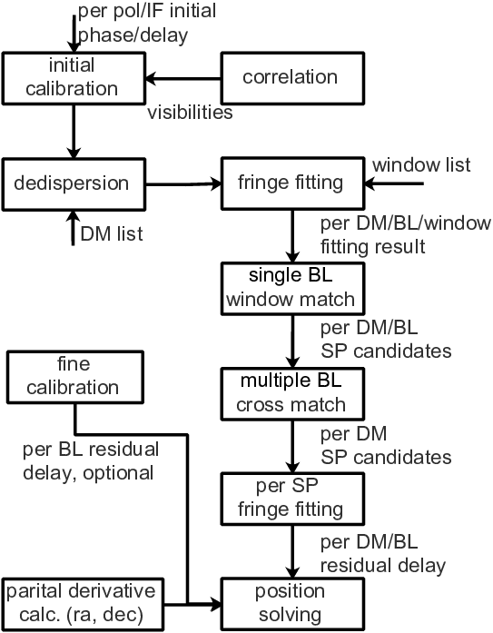
The detailed introduction to the VOLKS2 pipeline has been given in Liu et al. 2018a; Liu et al. 2019. Significant improvements have been made since the first release of the pipeline. Fig. 1 present the data flow of current pipeline. In this section, we will focus on the updates of the pipeline and the underlying algorithms.

Refer to caption — Figure 1: Data flow of VOLKS2 pipeline. Visibilities are first loaded into memory for all baselines (BLs) in a given time range. Then initial calibration is carried out for every polarization and IF (Intermediate Frequency). Then visibilities from multiple polarizations are combined together. Dedispersion is carried out for every DM (Dispersion Measure). After fringe fitting, single baseline window matching and multiple baselines cross matching, a single pulse (SP) list is obtained for each DM. For every single pulse, residual delay of each baseline is derived via fringe fitting. Finally the offset to a priori position is derived with geodetic VLBI solving.

II.1 Calibration

The calibration is divided into two parts, namely initial calibration and fine calibration.

II.1.1 Initial calibration

The purpose of initial calibration is to correct the initial delay $\Delta\tau_{0}^{n}$ and phase $\Delta\phi_{0}^{n}$ for every IF ( $n$ for IF index), baseline and polarization. The calibration values (delay and phase) are derived by carrying out fringe fitting on the strong calibration source. We assume these quantities reflect the status of the VLBI system and are kept unchanged across the observation. Fig. 2 demonstrates the fringe phase before and after initial calibration for the calibration source itself. The large IF delay is mainly due to station clock offsets. The discrepancies of initial delay and phase between IFs are small, however still exist. After calibration, fringe phase become flat and aligned across IFs.

II.1.2 Fine calibration

Fine calibration is carried out with reference sources close to the target. We assume the position of the reference source is accurate. Therefore the non-zero residual delay across all IFs (upper panel of Fig. 3) is caused by instruments and atmosphere. For each baseline, a residual delay is fitted. The fitting scheme is identical to the target source as described in Sec. II.2. The fitted value will be used to correct the baseline residual delay. Unlike phase reference calibration which requires delay, delay rate and phase information, fine calibration uses only delay information. This is demonstrated in Eq. 2 of Sec II.3.

II.2 Fringe fitting

Fig. 4 presents the cross spectrum (fringe phase and amplitude) of a single pulse detected in the pulsar observation. Following the Mk4 format adopted in the geodetic VLBI post processing package HOPS³³ 3 https://www.haystack.mit.edu/haystack-observatory-postprocessing-system-hops, the amplitude of each frequency point is normalized with the auto spectrum dispersion of the two stations: $|\widetilde{s_{ij}}|=|s_{ij}|/(\bar{a_{i}^{2}}\bar{a_{j}^{2}})^{1/4}$ . We would like to demonstrate that the fringe fitting process is effective in extracting single pulses from background noise. In this example, the fringe phase is clearly detected with just 4 milliseconds integration. A detailed explanation of the procedure is presented in Liu et al. 2018a. For the target single pulse search scan, the length of APs⁴⁴ 4 AP is short for accumulation period. In VLBI data processing it refers to visibilities within one integration period and IF. are in the level of milliseconds. E.g., 1.024 ms for EL060. For each baseline, several APs are summed together along the time axis to construct time segments with given window sizes. Fringe fittings are carried out for those time segments in each window. Window sizes are set to be comparable with the pulsar width. E.g., for PSR J0332+5434, pulsar width is around 7 ms. The corresponding window sizes are 2 ms, 4 ms, 8 ms, 16 ms. A single pulse is regarded as detected if it appears in at least 2 windows.

One thing we have to emphasis is the slightly different fringe fitting scheme. In Liu et al. 2018a, standard geodetic VLBI fringe fitting is used, which involves searching two quantities namely single-band and multi-band delay. However this scheme is designed for legacy system, in which the bandwidth of each IF is much narrower than IF intervals. In the typical astrophysical observation and in the next generation geodetic VLBI system (Petrachenko et al. 2013, VGOS,), IFs are much wider and always continuous. After calibration, it is more suitable to treat them as one fringe. Therefore, in VOLKS2, we search only one delay $\Delta\tau$ across all IFs inside the given band:

\displaystyle G(\Delta\tau)=\sum_{n=0}^{N-1}\sum_{j=1}^{J-1}S(n,j)e^{-i\Phi(n,j)}

with

	$\displaystyle\Phi(n,j)$	$\displaystyle=$	$\displaystyle 2\pi(f_{0}^{n}+f_{j}-f_{\mathrm{ref}})\Delta\tau$		(1)
		$\displaystyle+$	$\displaystyle 2\pi f_{j}\Delta\tau_{0}^{n}+\Delta\phi_{0}^{n},$		(1)

where $G(\Delta\tau)$ represents the searching function of the corresponding time segment $S$ , $f_{j}$ is the $j$ th frequency point in the $n$ th IF, $f_{\mathrm{ref}}$ is the reference frequency for fringe fitting, $\Delta\tau_{0}^{n}$ and $\Delta\phi_{0}^{n}$ are the initial delay and phase calibration values of the corresponding IF.

In the actual implementation, delay search is carried out with Fast Fourier Transform (FFT). To reduce the effect of cyclic convolution, padding is required. We choose a padding factor of 4 in the current pipeline. Standard geodetic fitting scheme conducts 2-D FFT, which requires a memory size of at least 16 times (4 $\times$ 4) that of the actual data. VOLKS2 conducts 1-D FFT, which reduces memory consumption by a factor of 4. This is especially important for GPU (Graphics Processing Unit) computing: compared with CPU, the size of GPU memory is quite limited. Lower memory consumption means we can initiate more computing context within one card, and therefore achieve higher performance. Moreover, current 1-D scheme provides much higher delay search resolution, which helps enhancing the SNR of the detected signal.

II.3 Localization

Localization is an important step in single pulse search. For VLBI observation, radio imaging method is usually adopted, such as the famous “realfast” pipeline (Law et al. 2015) that plays an important role in the first successful localization of repeating burst FRB121102. However, such kind of method carries out single pulse search in every snapshot, which is time consuming. As pointed out by Liu et al. 2019, by assuming the single pulse is a point source, it is possible to derive the single pulse position given the relation between the residual delay and the offset to a priori position. To improve the localization result, the single pulse fringe of each baseline must be calibrated. In the first release of VOLKS, this is conducted in AIPS. The pipeline at that time provides tools for preparing AIPS inputs and output. The calibration is conducted manually in AIPS.

For the design of VOLKS2, we want to get rid of the dependence of external software, and make the calibration and localization process simple and automatic. Therefore, we propose to conduct fine calibration, in which the residual delay is calibrated with the fringe fitting result of nearby reference sources:

\tau-\tau_{\mathrm{cal}}=\frac{\partial\tau}{\partial\alpha}\Delta\alpha+\frac{\partial\tau}{\partial\delta}\Delta\delta,

(2)

where $\tau$ and $\tau_{\mathrm{cal}}$ are the single pulse residual delay and the fine calibration delay for this baseline, $\frac{\partial\tau}{\partial\alpha}$ and $\frac{\partial\tau}{\partial\delta}$ are partial derivatives of delay by Ra and Dec at a priori position, $\Delta\alpha$ and $\Delta\delta$ are offsets to a priori position. The derived position is the a priori position corrected by offsets.

According to above equation, by assuming the single pulse as a point source and taking the idea of geodetic VLBI solving, we may derive the single pulse position with delay information only. This is different from phase reference calibration carried out by AIPS, which uses all information including delay, rate and phase. Compared with Eq. 2, phase reference calibration might be more accurate. However, it is more complicated and therefore not suitable for automatic implementation. Moreover, VOLKS2 pipeline is designed for regular VLBI observations, phase reference calibration requires the reference source close to the target source, which is not always available.

II.4 Performance improvement

The purpose of the VOLKS2 pipeline is to carry out single pulse search in VLBI observations. The designed running platform is modern GPU cluster. As the most time consuming part, fringe fitting is our concern for speedup. This part is both data and computationally intensive. First of all, loading data into memory is already a huge challenge: in EL060 which is used for single pulse search testing, the data size of a target search scan is around 650 GB (1.024 ms AP, 190 s duration, 7 stations, 21 baselines). In contrast, the memory size of one computing node is in the order of 100 GB. Even if using RAID to improve disk IO, the disk reading speed is still no higher than 1 GB/s. Moreover, the fitting process itself is time consuming: in the above scan, for one DM, we have to carry out 4 Million 32768 sized FFT and comparable number of matrix sum and finding maximum amplitude operations. To make the time consumption of fringe fitting acceptable, in the development stage, a lot of efforts have been made to improve the performance and to fully exploit the hardware resources, such as parallelization and code optimization.

II.4.1 Parallelization

The fringe fitting part of the pipeline is fully parallelized with MPI (Message Passing Interface). When the program starts, one assignment process and multiple calculation processes are initiated. The number of latter one depends on the CPU core number. For each scan, when a calculation process is idle, it sends task request to assignment process and obtains the time range. Then it loads the corresponding data into memory, carries out fringe fitting for all baselines in this time range, and saves the results in disk. This scheme is easy to understand and implement. No data communication is required between calculation processes, which keeps the architecture simple: the MPI part and the fringe fitting part are fully decoupled. When some processes are loading data, others carry out calculation. In this way the overhead of disk reading is reduced.

II.4.2 Code optimization

The fringe fitting part could be divided into 6 steps:

1.

Disk to memory. Load visibilities of give time range to memory.
2.

Baseline load. Load the required baseline data to the buffer array.
3.

Initial calibration. Carry out IF initial phase and delay calibration for buffer data.
4.

Dedispersion. For buffer data with given DM value.
5.

FFT. For each AP, carry out FFT along the frequency axis.
6.

Find max. For each window size, combining the FFTed APs along the time axis accordingly; find out the maximum amplitude along the delay axis (frequency axis after FFT) for each combined AP.

In the above steps, step 1 is conducted once for a given time range; step 2 - 6 are repeated for every baseline; step 4-6 are repeated for every DM value and baseline. To investigate the time consumption of each step, we carry out benchmarks. Fig. 5 demonstrates the result before GPU acceleration. All benchmarks in this work are carried out in a GPU server, of which the basic configuration is: Intel Xeon 5220R $\times$ 2 (48 cores in total), 48 TB data storage (RAID 4), 512 GB DDR4 memory, NVIDIA RTX 3080 $\times$ 1, RTX 2080Ti $\times$ 2.

In a computer system, disk IO is usually slow and is therefore the bottleneck. In DiFX (Deller et al. 2011), visibilities are stored in disk as records. To load the records of specific time range to memory, one has to find out the corresponding start and end indexes. Due to the high latency of each disk read request, it is not possible to go through all records in the disk sequentially. Noticing that visibility records are stored in chronological order, we implement a binary search routine, which is able to locate the target record with $\sim\log_{2}N$ read requests ( $N$ is the total number of records). This routine greatly reduces the records search time. However, the disk reading speed is still determined by the hardware configuration. As a result, the time consumption of step 1 is large and cannot be easily reduced. Fortunately this step is conducted only once. When averaged to every individual baseline and DM value, the portion is small.

After loading the records to memory, for each record, one has to parse the record header, find out the necessary information (time, polarization, baseline number, frequency), then copy the data to the right place in the buffer array. This is summarized as step 2, which involves a large number of conditional jump and memory read/write operations, and is usually not suitable for script languages such as Python. Therefore, we rewrite this part in C, compile it to dynamic loading library and call it in Python with “ctypes”. With this optimization, the time consumption of this step is reduced by an order (dotted and solid gray line in the figure), which makes the following optimization worthwhile.

After rewriting step 2 in C, the actual fringe fitting calculation, step 4 - 6 becomes the bottleneck. We use GPU to achieve further speedup. Two GPU computing frameworks, Torch and CuPy are used to call GPU resources. The benchmark is carried out with the NVIDIA RTX 3080 in the server. The result is demonstrated in Fig. 6. With the help of GPU, step 5 and 6 (FFT and Find max) achieve more than 2 orders speedup. The dedispersion step (step 4) is also accelerated when $t_{\mathrm{seg}}\geq 1$ s. However, the time consumption of this step does not change with data length. The reason is, for each frequency point, dedispersion invokes the GPU kernel once and applies a specific time shift to the data. In EL060 which is used for benchmark, the GPU kernel is invoked 8192 times. Since the time shift operation is simple, the kernel running time is negligible. However the accumulated kernel launch overhead, which is independent of data length, becomes significant. This part will be further optimized with the update of the pipeline.

One important parameter for optimization is the overall speedup. According to the analysis above, one may realize that the value depends on the specific application scenarios: for a typical configuration of EL060 (data length 4 s, 21 baselines), with known DM, the speedup is 7.9 X (209.1 s vs. 26.6 s). However, if DM search is required, in the case of 20 DM values, the speedup is 23.7 X (1876.1 s vs. 79.0 s). We would like to point out that some steps, e.g., initial calibration and dedispersion, can be further optimized, so as to achieve even higher speedup.

III Single pulse detection in EL060

We carry out single pulse detection with EL060 (EVN). The purpose of the observation is to verify the cross spectrum based single pulse detection scheme and the corresponding VOLKS2 pipeline. Main parameters of the observation are listed in Tab. 1. The observation is divided into pulsar part and RRAT (McLaughlin et al. 2007, Rotating Radio Transient, ) part. In general, single pulses are successfully detected and localized in the pulsar observation. However, no single pulse is detected in the RRAT observation. We will present detailed result and analysis in this section.

Table 1: Main parameters of EVN observation EL060.

Parameter	Setting
Experiment code	EL060
Observation date	Mar. 11, 2019 (MJD 58553)
Observation time	Start: 05h00m00s UTC
	Stop: 08h00m00s UTC
Station^a^aHh, Wb and Ef took part in RRAT observations only.	Wb, Ef, Mc, O8, Tr, Hh,
	Sv, Zc, Bd, Sr, Ir
Target	RRAT J1819 $-$ 1458, RRAT J1854 $+$ 0306
	PSR J0332 $+$ 5434
Initial calibration	J1800 $+$ 3848
Fine calibration	J1825 $-$ 1718, J1907 $+$ 0127, J0346 $+$ 5400
Polarization	L, R
Frequency	1594.49 MHz - 1722.49 MHz, 8 IFs
Bandwidth	16 MHz per IF
Sample bit	2

III.1 Pulsar observation

This part observes pulsar J0332 $+$ 5434 (B0329 $+$ 54). By placing the pulsar in the FoV with different offsets to the FoV center, we could investigate the detection efficiency and the localization accuracy in the whole FoV. The size (diameter) of the FoV is estimated as $\sim\lambda/D$ . $\lambda$ is set to 18 cm (L band) according to the observation. $D$ is the antenna diameter, a value of 32 m is selected, which is common for EVN stations (Mc, Tr, Ir, Sv, Zc, Bd). Above yield a FoV radius of $r$ = 9.7 arcmin. When preparing for the observation schedule, the pulsar is placed at 4 different places in the FoV by adjusting the offset between the pulsar and the antenna pointing center. The details of point centers together with the detection results at that place are listed in Tab. 2. Among those 4 pointing centers, P0 points to pulsar’s a priori position (Ra $03^{\mathrm{h}}32^{\mathrm{m}}59^{\mathrm{s}}.368$ , Dec $54^{\circ}34^{\prime}43^{\prime\prime}.57$ ). OF1, OF2 and OF3 point to 3 different offsets by adjusting declination only (right ascension is kept unchanged).

III.1.1 Detection rate

To evaluate the detection rate of each source under the same configuration, we exclude the Onsala (“O8”) station, since it is not available in the observation of OF2 and OF3. Moreover, for each scan, the on source time of each telescope is different. Therefore, we only include single pulses in the time range that all the considered stations are available for observation.

In total, we have 7 stations (Bd, Ir, Mc, Sr, Sv, Tr, Zc) that consist of 21 baselines. For each baseline, several APs are summed together along the time axis to construct time segments of different window sizes. We choose window sizes of 2, 4, 8, 16 APs. A single pulse is assumed to be detected when it fulfills the follow criterion:

•

For the time segments series of given window size, a single pulse is selected if its normalized power exceeds the threshold, which is set to 3 in this observation.
•

For a give baseline, match single pulses from 4 windows. A single pulse is selected if it appears in at least 2 windows.
•

Cross match single pulses from multiple baselines. A single pulse is identified if it is detected with at least 5 baselines.

Note that above criterion, together with the selection of windows sizes, could be adjusted according to observation.

According to Tab. 2, for each target, we calculate the total observation time and the “expected” single pulse number. Once a single pulse is detected, we could differentiate whether it is from the pulsar based on its pulsar phase. Real signals from pulsar and RFIs are labeled as “detected” and “invalid”, respectively. We get lower detection rate and invalid rate when the pulsar is close to the FoV center (P0 and OF1). However this does not agree with our expectation: central region of the FoV means higher antenna response, which should yield higher detection rate. By investigating the SNR as a function of time, the decrease of SNR in one of the P0 scan is observed in almost all baselines, which suggest that this is due to the flux variation of the pulsar. The most possible explanation of this phenomenon is refractive interstellar scintillation, which is caused by the small scale density fluctuations and appears as flux density variations in both time and frequency domains. According to Wang et al. 2008, the scintillation time scale of PSR J0332+5434 is 17.1 minutes, which is consistent with the dwelling time of each pointing center. Therefore, our postulation is the detection efficiency is roughly constant in the whole FoV. The variation of detection efficiency from 70% to 90% is mainly caused by interstellar scintillation.

Table 2: Parameters of 4 pointing centers and the corresponding detection results. “Offset” is in the fraction of FoV radius. The right ascension of the 4 point centers is set to

03^{\mathrm{h}}32^{\mathrm{m}}59^{\mathrm{s}}.368

and is kept unchanged.

Pointing center	Offset	Dec	Data length	Expected	Detected	Invalid
P0	0.0	$54^{\circ}34^{\prime}43^{\prime\prime}.57$	340 s	476	345 (72.5%)	1 (0.3%)
OF1	0.2	$+1^{\prime}56^{\prime\prime}.02$	340 s	476	424 (89.1%)	16 (3.6%)
OF2	0.5	$+4^{\prime}50^{\prime\prime}.06$	360 s	503	406 (80.7%)	0 (0.0%)
OF3	0.9	$+8^{\prime}42^{\prime\prime}.11$	306 s	429	388 (90.4%)	0 (0.0%)

III.1.2 Localization accuracy

For single pulses detected with above criterion, we carry out localization using the method described in Liu et al. 2019. As an improvement of the pipeline, fine calibration is proposed and introduced in Sec. II.3. When processing the data, we find that some further refinements are required to give reasonable localization result. First of all, Bd related baselines are excluded. In this work, the delay search range and the related FFT size is configured for projected baselines shorter than 3000 km. Bd related baselines exceed this limit. We can still detect single pulses with these baselines. However, due to the ambiguity of the delay search range, the fitted residual delay cannot be used for localization. Second, baselines with lower SNRs are excluded. For localization, visibilities that contain the single pulse signal are extracted and fringe fitted again by following the normalization and fitting procedure used in HOPS. Besides a more accurate fitting result, SNR is derived accordingly. We take a threshold of SNR $>$ 6, which is similar as that adopted in geodetic VLBI solving. For each single pulse, we exclude baselines that do not fulfill the above two requirements. Those with at least 3 baselines are used for localization.

We have to point out that one additional data point (OF3, Scan 40, 31.996 s, Mc-Sr baseline), is excluded from position solving. Although its SNR is high enough, the fitting result is wrong (probably due to RFI). The position of the corresponding single pulse solved by including this baseline deviates significantly from that of other single pulses. Actually this feature can be used to identify the incorrect baseline fitting result:

•

For the given single pulse, carry out solving several times, each time exclude one baseline;
•

Check the solving result, solution that includes the incorrect baseline fitting result deviates significantly from other solutions.

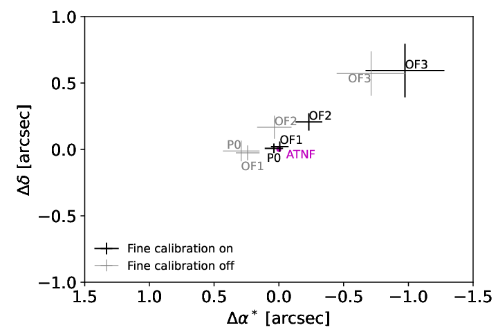
Fig. 7 demonstrates the localization result. By placing the pulsar in the FoV with different offsets to the pointing center, we may investigate the corresponding localization accuracy. Clearly larger offset yields larger discrepancy and scatter. This can be explained with the underlying algorithm of geodetic VLBI solving: the linear relation between the position offset and the delay is valid only if the target is close enough to a priori position (small offset). As the offset becomes large, the linear approximation is not enough to describe its relation with delay, which leads to the large discrepancy. Meanwhile, scatters are amplified correspondingly. Also note that in EL060, the offset is always along the declination direction, thus leads to the systemic trends of discrepancy. In Fig. 7, we present the localization result with and without fine calibration. A systematic shift is clearly observed between the two data sets. With calibration, localization result derived with P0 as pointing center becomes closer to the reference position, which is consistent with our analysis: small offset yields small discrepancy. This also proves that although simple and therefore easy to implement, our fine calibration scheme is effective in improving the localization accuracy. In summary, the localization discrepancy is around 1 arcsec when the target appears at the edge of the FoV, and quickly goes to well within 100 mas at the FoV center.

III.2 RRAT observation

In this part, we observe RRAT source J1819 $-$ 1458 and J1854 $+$ 0306, so as to verify the DM search capability of the pipeline. However, in the 80 minutes observation of 2 RRAT sources, no single pulse is detected. According to RRAT catalog⁵⁵ 5 http://astro.phys.wvu.edu/rratalog/, the flux and width of the RRAT sources, in particular J1854 $+$ 0306, are quite similar with that of pulsar J0332 $+$ 5434. It is unreasonable that all single pulses are missed. Our first suspicion is the newly developed pipeline. Therefore, we extract the auto spectrum of each station from the visibility output of the correlator, convert them to the filterbank format, and carry out single pulse search with STEP. The STEP transient search pipeline (Xu et al. 2021, in preparation) is developed in SHAO and tested using the ASKAP FRB data (Shannon & Bannister 2018). In particular, since Ef and Sr are larger than other telescopes, higher sensitivities are expected. Their data are further inspected by eyes. However, we are still not able to detect any single pulse.

By looking up references, one may find that the detected burst rate of RRAT source strongly depends on telescope sensitivity. E.g., the L-band burst rates of J1854 $+$ 0306 are 8.9, 84 and 102 $\pm$ 10 per hour for Parkes (Keane et al. 2011), Arecibo (Deneva et al. 2009) and FAST (Lu et al. 2019), respectively. Moreover, the intensity of single pulse varies significantly with time. In some epoch, no single pulse is ever detected (Keane et al. 2011). Note that the size of Ef is larger than that of Parkes, we may expect a similar or higher detection rate. Paragi 2016 do report the detection of single pulse in the e-EVN data of J1819 $-$ 1458, which is the first target of EL060. However, in our observation Ef only observed the second target J1854 $+$ 0306 for 25 minutes. No single pulse is detected in that short session. One thing we have to admit is, the possibility that the failed detection is caused by the VLBI mode observation still cannot be excluded: in our current treatment, raw data is recorded with VLBI backend. The single pulse detection is based on the correlated auto spectrum. Direct recording in pulsar mode might yield better result.

IV Conclusion

In this work, we introduce the VOLK2 pipeline, which takes the idea of geodetic VLBI fringe fitting and carries out single pulse search in the VLBI cross spectrum. In the VOLKS2 pipeline, single pulses are identified by fully utilizing the cross spectrum fringe phase information. By filtering candidate signals with multiple window sizes inside one baseline and by cross matching with multiple baselines, RFIs are eliminated effectively. Compared with station based single pulse search pipelines, our pipeline does not require extra RFI flagging. Once single pulse is detected, its position could be derived by geodetic VLBI solving with reasonable accuracy. The pipeline is designed for the transient search and localization in regular VLBI observations, as well as single pulse detections with know target (repeating FRBs, pulsars, etc.) in dedicated VLBI observations.

To verify the pipeline and the underlying cross spectrum based single pulse search method, we carry out EVN observation EL060. By placing the target pulsar in the FoV with different offsets to the FoV center, the detection efficiency and localization accuracy are investigated. We postulate that the detection efficiency is roughly constant in the whole FoV. The variation could be explained with the flux change caused by interstellar scintillation. Moreover, higher localization accuracy is achieved when the single pulse appears in the FoV center. By utilizing fine calibration proposed in this work, a localization accuracy of better than 100 mas is achieved. Also in this observation, no single pulse from RRAT sources is detected. We postulate this is because the telescopes are not sensitive enough to typical RRAT pulses. Therefore some further investigation is still required.

To fully utilize the hardware resources of modern GPU clusters, the pipeline is parallelized with MPI. Moreover, some steps in the fringe fitting part are accelerated with GPU. Depends on the specific search requirement and hardware configuration, the pipeline achieves a speedup from 7 X to 23.7 X. One thing we want to point out is, some unique steps, “FFT” and “Find max”, of our cross spectrum based pipeline achieves remarkable speedup ( $>$ 100 X) with the use of GPU, which makes their time consumption negligible compared with that of disk read and dedispersion. This suggest that with proper optimization, the cross spectrum based pipeline could run as fast as the popular auto spectrum based pipeline.

All the code and document are available in GitHub repository ⁶⁶ 6 https://github.com/liulei/volks2. We hope the VOLKS2 pipeline is useful for radio transient studies.

LL would like to thank Dr. Wu Jiang for his kind support in preparing and processing of the observation data. This work is supported by the National Natural Science Foundation of China (Grant Nos. 11903067, 12041301, U2031119, 11973011), CAS Key Technology Talent Program, Shanghai Leading Talents program, National Basic Public Science Data Center “Radio astronomy and deep-space exploration database” (NBSDC-DB-11), Natural Science Foundation of Shanghai (Grant No.20ZR1467600). The European VLBI Network (www.evlbi.org) is a joint facility of independent European, African, Asian, and North American radio astronomy institutes. Scientific results from data presented in this publication are derived from the following EVN project code: EL060.

References

(1)
Amiri et al. (2018) The CHIME/FRB Collaboration, Amiri, M., Bandura, K., et al. 2018, ApJ, 863, 48
CHIME/FRB Collaboration et al. (2020) CHIME/FRB Collaboration, Andersen, B. C., Bandura, K. M., et al. 2020, Nature, 587, 54.
CHIME/FRB Collaboration et al. (2021) CHIME/FRB Collaboration, Amiri, M., Andersen, B. C., et al. 2021, arXiv:2106.04352
Bochenek et al. (2020) Bochenek, C. D., Ravi, V., Belov, K. V., et al. 2020, Nature, 587, 59.
Caleb et al. (2016) Caleb, M., Flynn, C., Bailes, M., et al. 2016, MNRAS, 458, 718
Chatterjee et al. (2017) Chatterjee, S., Law, C. J., Wharton, R. S., et al. 2017, Nature, 541, 58
Clery (2020) Clery, D. 2020, Science, 370, 274.
Deller et al. (2011) Deller, A. T., Brisken, W. F., Phillips, C. J., et al. 2011, PASP, 123, 275
Deneva et al. (2009) Deneva, J. S., Cordes, J. M., McLaughlin, M. A., et al. 2009, ApJ, 703, 2259.
Keane et al. (2011) Keane, E. F., Kramer, M., Lyne, A. G., et al. 2011, MNRAS, 415, 3065.
Law et al. (2015) Law, C. J., Bower, G. C., Burke-Spolaor, S., et al. 2015, ApJ, 807, 16
Li et al. (2021) Li, C. K., Lin, L., Xiong, S. L., et al. 2021, Nature Astronomy.
Liu (2021) Liu, L. 2021, VOLKS2: VLBI Observation for single pulse Localization Keen Searcher, 2nd release, v0.7, Zenodo, doi:10.5281/zenodo.5168951
Liu et al. (2018a) Liu, L., Tong, F., Zheng, W., Zhang, J., & Tong, L. 2018a, AJ, 155, 98
Liu et al. (2018b) Liu, L., Zheng, W., Yan, Z., & Zhang, J. 2018b, Research in Astronomy and Astrophysics, 18, 069
Liu et al. (2019) Liu, L., Jiang, W., Zheng, W., Yan, Z., Zhang, J., Ma, M., & Luo, W. 2019, AJ, 157, 138
Lorimer et al. (2007) Lorimer, D. R., Bailes, M., McLaughlin, M. A., Narkevic, D. J., & Crawford, F. 2007, Science, 318, 777
Lu et al. (2019) Lu, J., Peng, B., Liu, K., et al. 2019, Science China Physics, Mechanics, and Astronomy, 62, 959503.
Manchester et al. (2005) Manchester, R. N., Hobbs, G. B., Teoh, A., & Hobbs, M. 2005, AJ, 129, 1993
Marcote et al. (2017) Marcote, B., Paragi, Z., Hessels, J. W. T., et al. 2017, ApJ, 834, L8
McLaughlin et al. (2007) McLaughlin, M. A., Rea, N., Gaensler, B. M., et al. 2007, ApJ, 670, 1307
Mereghetti et al. (2020) Mereghetti, S., Savchenko, V., Ferrigno, C., et al. 2020, ApJ, 898, L29.
Paragi (2016) Paragi, Z. 2016, arXiv:1612.00508
Petrachenko et al. (2013) Petrachenko, W., Behrend, D., Hase, H., et al. 2013b, EGU General Assembly Conference Abstracts, 15, EGU2013-12867
Prabu et al. (2020) Prabu, S., Hancock, P., Zhang, X., et al. 2020, PASA, 37, e052.
Ransom (2011) Ransom, S. 2011, Astrophysics Source Code Library.
Shannon & Bannister (2018) Shannon, R. & Bannister, K. 2018, Data from the ASKAP latitude 50 Fast Radio Burst (FRB) sample. v3. CSIRO. Data Collection.
ter Veen et al. (2019) ter Veen, S., Enriquez, J. E., Falcke, H., et al. 2019, A&A, 621, A57.
Wang et al. (2008) Wang, N., Yan, Z., Manchester, R. N., et al. 2008, MNRAS, 385, 1393
Wayth et al. (2011) Wayth, R. B., Brisken, W. F., Deller, A. T., et al. 2011, ApJ, 735, 97
Yuan et al. (2020) Yuan, Y., Beloborodov, A. M., Chen, A. Y., et al. 2020, ApJ, 900, L21.
Zhang et al. (2020) Zhang, C. F., Jiang, J. C., Men, Y. P., et al. 2020, The Astronomer’s Telegram, 13699
Zheng (2015) Zheng, W. 2015, IAU General Assembly, 22, 2255896