\JournalSubmission

Dynamic Diffuse Global Illumination ResamplingVolume: 40Issue: 4

Zander Majercik¹, Thomas Müller¹, Alexander Keller¹, Derek Nowrouzezahrai², and Morgan McGuire³
¹NVIDIA ²McGill University ³Roblox

Abstract

Interactive global illumination remains a challenge in radiometrically- and geometrically-complex scenes. Specialized sampling strategies are effective for specular and near-specular transport because the scattering has relatively low directional variance per scattering event. In contrast, the high variance from transport paths comprising multiple rough glossy or diffuse scattering events remains notoriously difficult to resolve with a small number of samples. We extend unidirectional path tracing to address this by combining screen-space reservoir resampling and sparse world-space probes, significantly improving sample efficiency for transport contributions that terminate on diffuse scattering events. Our experiments demonstrate a clear improvement – at equal time and equal quality – over purely path traced and purely probe-based baselines. Moreover, when combined with commodity denoisers, we are able to interactively render global illumination in complex scenes.

ccs

Computing methodologies Ray tracing

^†^†year: 2021^†^†year: 2021^†^†editors: A. Bousseau and M. McGuire^†^†subject: Eurographics Symposium on Rendering CGF Vol No ^†^†teaser: Ours + Denoising Offline Reference \begin{overpic}[figures/fig_teaser/combined_greek_villa.jpg] \put(38.54167,35.15625){\pic@makebox@{\makebox}{}(0.0,0.0){\hbox to37.18pt{\vbox to15.83pt{\pgfpicture\makeatletter\hbox{\hskip 0.8pt\lower-0.8pt\hbox to0.0pt{\lxSVG@begingroup@{_scopebegin} \lxSVG@begingroup@{stroke} \lxSVG@begingroup@{fill} \lxSVG@setlinewidth{\the\pgflinewidth}\lxSVG@begingroup@{stroke-width} \lx@inpgf@ignorespaces\nullfont\hbox to0.0pt{\lxSVG@begingroup@{_scopebegin} {}{{}}{} {\lx@inpgf@ignorespaces}{{}}{}{}{}{}{{}}{}\lxSVG@begingroup@{_scopebegin} \color[rgb]{1,0,0}\lxSVG@setlinewidth{\the\pgflinewidth}\lxSVG@begingroup@{stroke-width} \lx@inpgf@ignorespaces{}\lxSVG@stroke\lxSVG@drawpath@unclipped{M 0 0 M 0 0 L 0 19.69 L 49.23 19.69 L 49.23 0 Z M 49.23 19.69}{fill:none} \lx@inpgf@ignorespaces \lxSVG@closescope \lxSVG@closescope {\lx@inpgf@ignorespaces}{\lx@inpgf@ignorespaces}{\lx@inpgf@ignorespaces}\hss}\lxSVG@discardpath\lxSVG@closescope \hss}}\lxSVG@closescope\endpgfpicture}}}} \put(35.10417,22.91667){\pic@makebox@{\makebox}{}(0.0,0.0){\hbox to37.18pt{\vbox to15.83pt{\pgfpicture\makeatletter\hbox{\hskip 0.8pt\lower-0.8pt\hbox to0.0pt{\lxSVG@begingroup@{_scopebegin} \lxSVG@begingroup@{stroke} \lxSVG@begingroup@{fill} \lxSVG@setlinewidth{\the\pgflinewidth}\lxSVG@begingroup@{stroke-width} \lx@inpgf@ignorespaces\nullfont\hbox to0.0pt{\lxSVG@begingroup@{_scopebegin} {}{{}}{} {\lx@inpgf@ignorespaces}{{}}{}{}{}{}{{}}{}\lxSVG@begingroup@{_scopebegin} \color[rgb]{1,0.5,0}\lxSVG@setlinewidth{\the\pgflinewidth}\lxSVG@begingroup@{stroke-width} \lx@inpgf@ignorespaces{}\lxSVG@stroke\lxSVG@drawpath@unclipped{M 0 0 M 0 0 L 0 19.69 L 49.23 19.69 L 49.23 0 Z M 49.23 19.69}{fill:none} \lx@inpgf@ignorespaces \lxSVG@closescope \lxSVG@closescope {\lx@inpgf@ignorespaces}{\lx@inpgf@ignorespaces}{\lx@inpgf@ignorespaces}\hss}\lxSVG@discardpath\lxSVG@closescope \hss}}\lxSVG@closescope\endpgfpicture}}}} \end{overpic}

Path tracing + ReSTIR + Secondary DDGI (ours) + DDGI Resampling (ours) + Denoising (ours) Reference 22.5 ms 12.8 ms 18.4 ms 26.6 ms The indirectly lit Greek Villa scene rendered at

1920\times 1080

with 1 sample per pixel (spp) on an i7 6800k CPU and RTX 3090 GPU. Direct illumination resampling, such as ReSTIR [BWP*20] (leftmost inset), reduces noise at the primary path vertex but does not affect the remainder of the path which is both noisy and expensive to trace. Therefore, we propose replacing the remainder of the path, starting from the secondary vertex, with a cheap, noise-free approximation: an extended variant of DDGI [MMSM21] (second inset). Our key observation is that DDGI thereby acts as a light source, allowing us to include it in the resampling algorithm (third inset). This unifies the sampling of direct and indirect illumination. Combined with denoising (fourth inset), scenes with complex indirect illumination such as this one can be rendered in real time from 1 spp, with quality approaching offline path tracing with hundreds of samples per pixel (fifth inset).

1 Introduction

Modern physically-based production renderers rely primarily on variants of the unidirectional path tracing algorithm [Bal18], in which paths are traced from the camera and scattered in the scene until they reach an emitter. Path tracing scenes with high geometric and radiometric complexity can result in high-variance (i.e., noisy) images unless they take a prohibitively large number of samples. To alleviate this, many Monte Carlo variance reduction-based solutions have been proposed, such as variants of importance sampling [VG95, OZ98, TCE05, BWP*20] and path guiding [VHH*19]. However, even with advanced sampling techniques in place, hundreds of samples per pixel are typically required to produce a converged image, which is prohibitive for real-time applications.

Even though recent improvements in GPU ray tracing and effective denoising have greatly improved path tracing performance for complex scenes, real-time path tracing budgets remain limited to only few indirect scattering events (often just one) and scenes with only modestly complex illumination. As such, interactive graphics methods necessarily resort to approximate global illumination methods in addition to importance sampling. One such recent approach combines world-space irradiance probes with visibility-aware interpolation to rapidly approximate multi-bounce indirect illumination (DDGI) [MGNM19]. Crucially, the normal-dependent irradiance can also be interpreted as cosine-prefiltered radiance [MMSM21] in the normal direction, allowing its use in both rough glossy as well as Lambertian diffuse transport. As with most approximate solutions, these dynamic probes introduce bias – in the form of the transport that is computed – in exchange for a noise-free and fast result.

In contrast to interactive indirect illumination sampling, the sample efficiency and approachable scene complexity for ray-traced direct illumination has been greatly improved by recent a spatio-temporal resampling scheme (ReSTIR) [BWP*20]. In the graphics pipeline, sampling is followed by full-screen post-processing, including denoising [BRM*16, BB17, SKW*17, VRM*18, BVM*17, CKS*17, MMBJ17, XZW*19, HY21]. So, the goal of a modern real-time sampling algorithm is not a fully converged image, but rather one with sufficiently low noise that after post-processing it is acceptably close to a converged image for the application. We address the efficient sampling problem in this work, assuming a downstream denoiser. We note that today’s commodity denoisers both desirably conceal sampling noise and also undesirably exhibit various residual temporal errors that are beyond the scope of this work. Hence, we show the impact of denoising in Fig. for a static image to validate the unconverged targets, and then show the pre-denoising output of our method in all other results.

We present a new real-time global illumination method that combines the advantages of spatio-temporal resampling (improved sample efficiency for stochastic estimators) and dynamic diffuse probe volumes (smooth, interpolation-friendly transport proxies). Our method is efficient, treats direct and multi-bounce indirect effects, and is robust to radiometrically- and geometrically-complex settings. Naïvely combining DDGI with ReSTIR (see Fig. 7, “Primary DDGI” column) will neither eliminate the probe grid artifacts nor address the discrepancy in their respective artifact/noise characteristics: DDGI’s noise-free and biased indirect illumination, and ReSTIR’s noisy and unbiased direct illumination.

We alleviate this discrepancy by postponing DDGI queries by one bounce (from the eye) – where sample contributions are evaluated during ReSTIR (see Fig. 7, “DDGI in ReSTIR” column) – similarly to final gathering with photon mapping [Jen96]. This hides a large portion of DDGI’s bias and allows us to combine direct and indirect samples during resampling, selecting each sample proportional to its global transport contribution. Where the original ReSTIR approach would normally resample direct illumination, it now treats both direct and indirect samples, each with similar noise characteristics due to the final gathering-like postponed DDGI sample, resulting in a sample efficient global shading estimate that is amenable to commodity denoising methods (see Fig. ).

Our method takes a principled approach to balancing the performance-quality trade-off inherent to any combination of DDGI and ReSTIR, as evidenced in our analysis and benchmark against purely path traced and purely probe-based variants (Sec. 5). Concisely, our contributions are as follows:

•

a categorization of contributions from each constituent technique,
•

an in-depth analysis of sampling-based methods applied to these contributions,
•

an interactive global illumination algorithm, motivated by our analysis, that combines resampling with a global transport approximation.

2 Background and Related Work

(Ir)radiance Caching.

Most modern real-time global illumination caches have their roots in Ward’s seminal irradiance cache [WRC88] and other early approaches to precomputed light transport [Arv86, Hec90]. While initial work focused on adapting precomputed light transport to the harsh constraints of real-time rendering in static settings [Abr97, Oat05, ME10], many recent techniques offer at least partial dynamics, such as dynamic lighting through precomputed radiance transfer [SKS02]. Orthogonally, radiance caching techniques overcome the Lambertian assumption by including the directional domain [KGPB05]. Although today’s selection of high-quality partially dynamic techniques is vast [GS12, SL17, SSS*20, VPG14, SNRS12, RZD14, SJJ12], our goal is fully dynamic global illumination with as few constraints as possible.

To this end, we build upon the DDGI volume [MGNM19], which consists of a 3D grid of directionally resolved irradiance probes that is updated in real-time through hardware ray-tracing. Crucially, DDGI contains visibility information to prevent light leaking and it can approximate sufficiently rough glossy transport by re-purposing its directional dependence [MMSM21]. These features make it – with mild modifications (Sec. 3) – a reasonably versatile approximation of global illumination for most phenomena other than specular reflections. By querying DDGI at secondary path vertices, we employ a similar strategy to final gathering to conceal DDGI’s limitations (e.g., coarse spatial discretization) behind the blurring effect of the primary scattering interaction at the cost of sampling noise. We then address the sampling noise by applying spatio-temporal reservoir sampling [BWP*20].

Müller et al. [MRNK21] use a real-time trained neural radiance cache to approximate fully-dynamic global illumination. They evaluate their cache at later path vertices to hide the artifacts of their neural network, but unlike this paper, they do not employ specialized importance sampling. Crucially, their method is compatible with ours in that the caches can be interchanged in future investigations.

Importance Sampling.

In offline rendering, importance sampling is the dominant technique for reducing sampling noise: the closer the sampling distribution matches the distribution of light, the less noise there is [Vea97]. With the advent of hardware ray tracing, it is now important to adapt established techniques to the real-time setting [KVB*19].

Like with caching techniques, spatio-temporal reuse is key for high-quality importance sampling, as evidenced by bidirectional techniques [LW93, VG94, VG97, Kel97, GKDS12], resampling and mutation strategies [TCE05, VG97, KSAC02, KMA*15, HKD14], as well as learned distributions via neural networks [MMR*19, ZZ19, KD19] or path guiding [Jen95, LW95, VKŠ*14, MGN17, DK18]. Unfortunately, most reuse strategies come with a significant performance penalty, meaning that while they handle difficult illumination well, they are outperformed by naïve unidirectional path tracing under simple illumination. This disqualifies them from the real-time setting that we strive for. Path guiding has generally little overhead, which makes it a good choice for production rendering [VHH*19], however adapting its underlying data structures to animated content in real-time is non-trivial ongoing work [DHD20].

Our importance sampling method of choice is ReSTIR [BWP*20]: a recent combination of importance resampling [TCE05] and classic weighted reservoir sampling [Vit85, ES06, CHA82] that permits the reuse of a massive number of samples in constant time. For estimating direct lighting, ReSTIR generates many candidate samples on the light sources in the scene, resamples those candidates across space and time proportional to their predicted contribution, and then traces a shadow ray to determine the visibility of the selected sample(s). This scheme not only has negligible overhead compared to simple path tracing, but also gracefully handles dynamic content.

In contrast, we apply ReSTIR to global illumination by targeting it at the sum of direct illumination from light sources and indirect illumination stored in DDGI probes [MGNM19] of irradiance (for diffuse reflection) and angularly-filtered radiance [MMSM21] (for rough glossy reflection). This converts the global illumination problem into a purely direct illumination problem for the high variance case of low-frequency angular scattering, by treating DDGI as a light source. In contrast to multiple importance sampling [VG95], this means that we draw a single sample approximately proportional to the total transported light rather than multiple samples that are heuristically combined. Note that the result has two symbiotic levels of reuse: (i) screen-space resampling by ReSTIR for both direct and indirect light as well as (ii) world space DDGI probes which contain spatio-temporal aggregates of global illumination.

Concurrent work of Ouyang et al. [OLK*21] proposes an alternative mechanism for spatio-temporal resampling of global illumination: they target ReSTIR at single-sample Monte Carlo estimates – rather than a cache – which can be likened to importance sampling of virtual point lights. Compared with our approach, theirs is capable of less biased (optionally unbiased) rendering, but lacks world-space spatio-temporal reuse and early path termination, which in our case is handled by the DDGI volume.

As we show in our results, combining the underlying ideas of ReSTIR, DDGI, and path tracing into a new sampling strategy produces a less-biased and less noisy result than naïvely compositing the results of separately-computed ReSTIR direct, DDGI diffuse/rough-glossy indirect, and path traced near-specular contributions.

3 Algorithm

In order to render images with global illumination in real-time, we strive to efficiently simulate radiance transport. The rendering equation [Kaj86]

L=L_{e}+T_{f}\;L

(1)

describes the outgoing radiance $L:\mathbb{R}^{3}\times\mathbb{S}^{2}\rightarrow\mathbb{R}^{3}$ as the sum of the radiance $L_{e}$ emitted by the light sources and the transported radiance $T_{f}L$ , where $T_{f}$ is a higher order operator that maps between two functions (similar to notation defined by Veach [Vea97]). The symbol $f$ represents the bidirectional scattering distribution function (BSDF), describing how the surfaces in the scene transport radiance. For our derivation, it is useful to partition radiance transport

T_{f}=T_{f_{\mathrm{d}}}+T_{f_{\mathrm{g}}}

into diffuse $T_{f_{\mathrm{d}}}$ and glossy $T_{f_{\mathrm{g}}}$ transport, the latter of which including specular transport as the special case of small surface roughness.

With this operator notation at hand, the dynamic diffuse global illumination (DDGI) algorithm [MGNM19] is

L\approx L_{e}+T_{f_{\mathrm{d}}}\;L_{e}+L_{\text{DDGI}}+T_{f_{\mathrm{g}}}\;L\;,

(2)

in which $L_{\text{DDGI}}\approx\sum_{i=2}^{\infty}(T_{f_{\mathrm{d}}})^{i}\;L_{e}$ is an approximation of the diffuse transported radiance without the directly visible light sources ( $i$ starts at 2). The other terms are estimated by sampling. Inserting the DDGI approximation into equation (2) and assuming equality results almost in the rendering equation (1), missing only higher order glossy transport.

Majercik et al. [MMSM21] extended DDGI to include this missing contribution for the special case of specular reflection, which we will build on in Section 3.3. The “Primary DDGI” column in Fig. 2 and 7 shows results of this extended DDGI algorithm. As compared to path tracing [Kaj86], the images are smooth and noise only results from sampling the direct diffuse illumination $T_{f_{\mathrm{d}}}\;L_{e}$ and the recursion for glossy transport $T_{f_{\mathrm{g}}}\;L$ . Yet, the irradiance probe approximation of $L_{\text{DDGI}}$ shows visible artifacts that we resolve by postponing its evaluation to secondary path vertices. We develop our new algorithm in the following sections.

Refer to caption — Figure 1: We compute direct and indirect illumination in a unified way by targeting the ReSTIR algorithm at the sum of emitted light $L_{e}$ and the DDGI approximation $L_{\text{DDGI}}$ . Left: two points are sampled. One (red) is sampled on the emissive surfaces and another (green, $\mathbf{y}$ ) by BSDF sampling at the primary vertex $\mathbf{x}$ . Right: with all samples across pixels and past frames converted to the area measure, a single sample $\mathbf{z}$ is selected with probability proportional to ${L_{e}+L_{\text{DDGI}}}$ and a shadow ray (red) is traced. The radiance leaving $\mathbf{x}$ towards the camera is estimated with low variance by combining the reflected light from $\mathbf{y}$ and $\mathbf{z}$ through the method of Kollig and Keller [KK06]. (Near-)specular transport at $\mathbf{y}$ and $\mathbf{z}$ is estimated through recursion (blue) and the remaining transport by $L_{\text{DDGI}}$ .

3.1 Sampling all Surfaces with ReSTIR

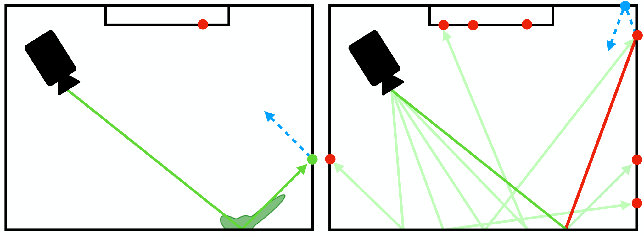
As the DDGI approximation can be queried at any point of the scene surface, we consider the whole scene surface as a light source rather than only the actual light sources. Our new sampling algorithm performs the following steps:

1.

Generate candidate samples on all surfaces of the scene. To this end, we uniformly sample a small number of positions on emissive surfaces and generate additional samples by tracing secondary rays in directions sampled from the BSDF.
2.

Select one candidate by first sampling from a weighted reservoir proportional to the sample contribution, then resample spatially among neighboring pixels, and resample temporally among previous frames, proportional to the sum ${L_{e}+L_{\text{DDGI}}}$ .
3.

Trace one shadow ray to the selected sample point.
4.

If visible, shade from that sample point, using the emissive contribution $L_{e}$ and adding the contribution from the DDGI volume.

As with original ReSTIR, our unified sampling scheme traces only a single ray to the selected sample (see Figure 1). However, as the original DDGI volume only contains the diffuse indirectly reflected light without direct reflections as shown in equation (2), we need to add these, as well as glossy contributions, which we describe next.

3.2 Augmenting the DDGI Approximation

As mentioned in Sec. 3.1, integrating $L_{\text{DDGI}}$ from secondary vertices over the hemisphere at the primary vertex would result in too dark images, because the DDGI approximation lacks the diffuse direct illumination and the radiance from non-diffuse transport. In fact, adding these missing terms to the DDGI approximation recovers an approximation of the transport operator

L_{\text{DDGI}}+T_{f_{\mathrm{d}}}\;L_{e}+T_{f_{\mathrm{g}}}\;L\approx T_{f_{\mathrm{d}}}\;L+T_{f_{\mathrm{g}}}\;L=T_{f}\;L.

(3)

Adding the missing terms by recursive path tracing would increase the noise and involve further shading and tracing cost.

Instead, we augment the DDGI approximation in two steps, which are most easily explained by examining the underlying irradiance approximation that DDGI makes. Given a 3D position and 2D normal vector, the DDGI probe volume stores irradiance from indirect diffuse reflections, which is approximated by repeatedly evaluating the following double-bounce transport [MGNM19]

	$\displaystyle E_{\text{DDGI}}(\mathbf{x},\mathbf{n})$	$\displaystyle\approx\int(L_{\text{DDGI}}+T_{f_{\mathrm{d}}}\;L_{e})(h(\mathbf{x},\omega_{\mathrm{i}}),-\omega_{\mathrm{i}})\langle\mathbf{n},\omega_{\mathrm{i}}\rangle\,\,\mathrm{d}\omega_{\mathrm{i}}\,,$
	$\displaystyle L_{\text{DDGI}}(\mathbf{x},\omega_{\mathrm{i}})$	$\displaystyle:=\frac{\rho(\mathbf{x})}{\pi}\;E_{\text{DDGI}}(\mathbf{x},\mathbf{n})\,,$		(4)

where $h$ is the ray tracing operation and $\rho$ is the diffuse albedo. Repeated Monte Carlo estimation of this equation at the centers $\mathbf{x}$ of all DDGI probes converges to the aforementioned approximation

L_{\text{DDGI}}\approx\sum_{i=2}^{\infty}(T_{f_{\mathrm{d}}})^{i}\;L_{e}\,.

To include direct reflections and non-diffuse transport, we replace the double-bounce transport with simpler single-bounce recursion

\displaystyle E_{\text{DDGI+}}(\mathbf{x},\mathbf{n})\approx\int(L_{\text{DDGI+}}+L_{e})(h(\mathbf{x},\omega_{\mathrm{i}}),-\omega_{\mathrm{i}})\langle\mathbf{n},\omega_{\mathrm{i}}\rangle\,\,\mathrm{d}\omega_{\mathrm{i}}\,,

(5)

where $L_{e}$ no longer undergoes a diffuse interaction and $L_{\text{DDGI+}}$ will be adapted to include glossy transport in the following section. The approximation thus converges to the full transport operator

L_{\text{DDGI+}}\approx T_{f}\;L\,.

Including direct illumination (i.e. untransported $L_{e}$ ) in the probe update equation (5) produces results that are too bright whenever probe centers are closer to light sources than the surfaces that they shade. This causes surfaces to receive more (secondary) direct illumination than they should – a common problem in probe-based caches. To alleviate this, we approximate the true distance to the surface by querying the average visibility already computed by the probes in the backwards direction [MGNM19] (dashed red lines), clipping that value to the probe boundary (pink), and adding it to the length of the corresponding probe update rays (solid red arrows). Because the update rays are traced per probe, this costs just a texture read without any probe weight computation.

We then use the inverse square of the total distance, i.e., solid + dashed, to attenuate $L_{e}$ . In contrast to direct illumination computed at probe centers, this heuristic slightly underestimates direct illumination. We therefore expose a user-tunable slider to scale the additional attenuation per scene to correct for brightness differences that would otherwise be a significant source of bias.

3.3 Including Glossy Illumination

Recall that the reflected light from a diffuse material with albedo $\rho$ can be cheaply approximated by looking up $\frac{\rho(\mathbf{x})}{\pi}\;E_{\text{DDGI+}}(\mathbf{x},\mathbf{n})$ .

Majercik et al. [MMSM21] make the observation that the irradiance approximation can additionally be used to very coarsely approximate specular transport by substituting the normal $\mathbf{n}$ with the direction of specular reflection $\omega_{\mathrm{r}}$ . The irradiance $E_{\text{DDGI}}(\mathbf{x},\omega_{\mathrm{r}})$ can then be re-interpreted as a prefiltered (by the cosine term) coarse approximation of incident radiance up to a normalization factor of $2\pi$ which must be added. In the illustration, the green lobes visualize cosine-weighted prefiltering of incident radiance and the red arrows indicate the query direction of $E_{\text{DDGI}}$ .

While Majercik et al. use this strategy for just specular transport, we generalize it to arbitrary glossy BSDFs – in our case microfacet models – by Monte Carlo estimation. More specifically, we approximate reflected radiance by our augmented DDGI model

	$\displaystyle L_{\text{DDGI+}}(\mathbf{x},\omega_{\mathrm{o}})$	$\displaystyle=\underbrace{\frac{\rho(\mathbf{x})}{\pi}\;E_{\text{DDGI+}}(\mathbf{x},\mathbf{n})}_{\text{Diffuse}}$		(6)
		$\displaystyle+\underbrace{\frac{1}{2\pi}\int E_{\text{DDGI+}}(\mathbf{x},\omega_{\mathrm{i}})f_{\mathrm{g}}(\mathbf{x},\omega_{\mathrm{o}},\omega_{\mathrm{i}})\langle\mathbf{n},\omega_{\mathrm{i}}\rangle\,\,\mathrm{d}\omega_{\mathrm{i}}}_{\text{Glossy}}$

as the decomposition into diffuse and glossy transport, where we estimate the glossy integral with a single Monte Carlo sample drawn proportionally to the glossy BSDF component $f_{\mathrm{g}}$ .

Specular recursion for shading.

We use our radiance approximaton $L_{\text{DDGI+}}$ in three parts of the algorithm: (i) in the update rule of $E_{\text{DDGI+}}$ (5), (ii) to resample proportional to ${(L_{e}+L_{\text{DDGI+}})}$ , and (iii) for shading. The latter use case – shading – requires special care to avoid exposing too much of the inherent bias of $L_{\text{DDGI+}}$ through (near-)specular interactions.

We thus trace shading paths recursively until their scattering footprint is sufficiently spread out to blur DDGI’s visual artifacts. To this end, we adopt the path termination strategy of Müller et al. [MRNK21, MRKN20], which is based on the isotropic path footprint approximation of Bekaert et al. [BSC*03].

More specifically, we approximate the footprint of a path with vertices $\mathbf{x}_{1}\cdots\mathbf{x}_{n}$ as

\displaystyle a(\mathbf{x}_{1}\cdots\mathbf{x}_{n})

\displaystyle={\mathopen{}\mathclose{{\left(\sum_{i=1}^{n-1}\sqrt{\frac{\|\mathbf{x}_{i}-\mathbf{x}_{i+1}\|^{2}}{p_{i}(\omega_{\mathrm{i},i}\,|\,\mathbf{x}_{i},\omega_{\mathrm{o},i})\,\langle\mathbf{n}_{i+1},-\omega_{\mathrm{i},i}\rangle}}}}\right)}^{2}\,,

(7)

where $p_{i}$ is the BSDF sampling density at the $i$ -th vertex. At the primary vertex, $p_{1}$ is proportional to the entire BSDF $f$ , whereas ${p_{i};\,i>1}$ is proportional to only the glossy portion of the BSDF $f_{\mathrm{g}}$ , because we simply terminate the recursion early and query $\frac{\rho(\mathbf{x}_{n})}{\pi}\;E_{\text{DDGI+}}(\mathbf{x}_{n},\mathbf{n}_{n})$ when the diffuse portion is sampled. When the glossy portion is sampled, we terminate the recursion by estimating the glossy integral of Eq. (6) as soon as $a(\mathbf{x}_{1}\cdots\mathbf{x}_{n})>a_{0}\cdot c$ , where

\displaystyle a_{0}:=\frac{\|\mathbf{x}_{0}-\mathbf{x}_{1}\|^{2}}{4\pi\;\langle\mathbf{n}_{1},-\omega_{\mathrm{i},i}\rangle}

(8)

is an approximation (up to constant factors) of the pixel footprint projected into the scene, $\mathbf{x}_{0}$ is the camera position, and $c$ is a user-chosen threshold. See Bekaert et al. [BSC*03] and Müller et al. [MRNK21, MRKN20] for details.

We empirically set the threshold ${c=0.2}$ to obtain a satisfactory noise versus bias trade-off. Fig. 3 confirms that this helps reduce artifacts on highly glossy surfaces without affecting rough glossy and diffuse surfaces.

3.4 Correcting Self-shadow Bias

The original DDGI algorithm applies an offset to the positions at which $L_{\text{DDGI}}$ is queried to avoid computing visibility weights exactly at a surface where their variance is high. This offset is called the “self-shadow” bias, and is computed as a weighted combination of the view and normal vector at the queried point.

While the self-shadow bias was sufficient for the original primary-vertex DDGI algorithm, using it unmodified in our indirect sampling strategy showed light leaking artifacts (Figure 4). These artifacts arise from very short distances between the view point and the query point, as might arise from sharp corners. To address these artifacts, we bias the query point along the view path as opposed to the surface normal and view direction. Results using our view path bias against the original self-shadow bias are shown in Figure 4.

3.5 Taming the Weak Singularity in the Geometry Term

In order to perform spatio-temporal resampling among different shading locations, the geometry term is introduced as part of the change of the integration measure. Unfortunately, the weak singularity in the geometry term may lead to unbounded variance in the resampling procedure in geometric creases; see Fig. 5 (middle).

In typical path tracing applications, uniform multiple importance sampling [VG95] of light sources would bound the variance when light sources (almost) touch the surfaces that they shade. But this is an impractical solution in our case, where the entire scene is considered a light source. It may be feasible to non-uniformly sample all relevant scene surfaces according to a data structure that is constructed online, but we instead take a simpler approach that does not require multiple importance sampling: we partition the integrand to bound the variance [KK06].

To avoid the weak singularity caused by samples very close to the primary vertex, we clamp the computed geometry term to a maximum value of $G_{\text{max}}=1$ and use the notation $\lceil T_{f}\rceil$ for the transport with this bounded geometry term. The residual transport is denoted by $\lfloor T_{f}\rfloor$ , such that

T_{f}=\lceil T_{f}\rceil+\lfloor T_{f}\rfloor.

$\lfloor T_{f}\rfloor$ is evaluated by an auxiliary BSDF sample in the sampling step described in Sec. 3.1. The improved variance is shown in Fig. 5.

In summary, our new algorithm to approximate the rendering equation amounts to summing separate estimators of each term of

L\approx L_{e}+\underbrace{\lceil T_{f}\rceil\;(L_{e}+L_{\text{DDGI+}})}_{\text{bounded geometry term}}+\underbrace{\lfloor T_{f}\rfloor\;(L_{e}+L_{\text{DDGI+}})}_{\text{residual transport}},

(9)

where

•

$L_{e}$ is evaluated at the primary vertex,
•

$\lfloor T_{f}\rfloor$ by importance sampling the BSDF, and
•

$\lceil T_{f}\rceil$ by spatio-temporal reservoir resampling.

3.6 Improved Performance by Caching DDGI Queries

During the spatio-temporal resampling step, our algorithm requires numerous DDGI queries: one for each candidate’s contribution to the shaded pixel, which, in our implementation, amounts to 1 temporal and 3 spatial candidates per pixel.

In the illustration, we depict the simpler case of resampling among just 2 spatial candidates $\mathbf{y}_{2}$ and $\mathbf{y}_{3}$ for shading at the center vertex $\mathbf{x}_{1}$ . For each candidate, we must query its contribution $L_{\text{DDGI+}}(\mathbf{y}_{i},\mathbf{y}_{i}\!\rightarrow\!\mathbf{x}_{1})$ to the center vertex, where ${\mathbf{y}\!\rightarrow\!\mathbf{x}}$ is the direction vector pointing from $\mathbf{y}$ towards $\mathbf{x}$ (dashed arrows).

These ${\text{\#vertices}\times\text{\#candidates}}$ queries can be avoided by approximating them with the #vertices values $L_{\text{DDGI+}}(\mathbf{y}_{i},\mathbf{y}_{i}\!\rightarrow\!\mathbf{x}_{i})$ , which have to be evaluated for shading each vertex $\mathbf{x}_{i}$ in any case. This saves a factor of #candidates queries. Importantly, using approximate values in the resampling step does not introduce additional bias in the rendered image – merely additional noise.

Nonetheless, we analyze the error of this approximation by considering its three sources:

1.

the scene and the DDGI volume may change each frame,
2.

the shading location $\mathbf{x}$ is different, and
3.

the view-path bias (Sec. 3.4) depends on the path prefix

each of which become small if we apply the assumptions of our method: local pixel neighborhoods, near-diffuse scattering, and short frame times. The approximation error is thus reasonably small in practice (see Fig. 6) and we use this optimization in all our results.

4 Results

We implemented DDGI resampling in Direct3D 12 using the Falcor rendering framework [BYC*20]. All results were generated on a high-end desktop machine with an Intel i7-6800K CPU and an NVIDIA RTX 3090 GPU.

Fig. 7 summarizes our results, comparing visuals, render time, and mean absolute percentage error (MAPE) of 5 different rendering techniques at 1 sample per pixel. MAPE is defined as $\frac{1}{N}\sum_{i=1}^{N}|v_{i}-\hat{v}_{i}|/(\hat{v}_{i}+\epsilon)$ , where $\hat{v}_{i}$ is the value of the $i$ -th pixel in the reference image, $v_{i}$ is the value of the $i$ -th rendered pixel, and $\epsilon=0.01$ prevents near-black pixels from dominating the metric.

All rendering techniques are based on an unbiased path tracer that uses ReSTIR [BWP*20] to estimate direct illumination at the primary vertex.

1.

PT + ReSTIR: The aforementioned baseline path tracer.
2.

Primary DDGI: The original DDGI algorithm [MGNM19, MMSM21], which approximates indirect illumination at the primary vertex of the path.
3.

Secondary DDGI: Our augmented DDGI algorithm approximates global illumination at the secondary vertex of the path (Sec. 3.2–3.4). Near-specular transport is traced recursively.
4.

+ DDGI in ReSTIR: The same as before, but the DDGI approximation is included in the ReSTIR algorithm (Sec. 3.1). The diffuse weak singularity is separately sampled (Sec. 3.5).
5.

+ Denoising: The same as before, but with OptiX denoising.

As expected, the DDGI algorithm [MGNM19, MMSM21] has the least noise with the greatest performance (“Primary DDGI” column). However, it also exhibits significant visual artifacts such as flat shading (e.g., in the Greek Villa), a lack of ambient occlusion (e.g., in the Pink Room), and light leaking (e.g., in the Living Room). At the other extreme, an unbiased path tracer produces highly accurate results but requires a long time for its noise to converge away in globally illuminated scenes, even when using ReSTIR [BWP*20] for direct lighting (“PT + ReSTIR” column).

Table 1: Time to converge to equal MAPE

Scene	Method	Frames	Time	MAPE
Greek Villa	PT+ReSTIR	129	2908.00 ms	0.573
	+Secondary DDGI	8	113.52 ms	0.578
	+DDGI Resampling	1	19.83 ms	0.572
Living Room	PT+ReSTIR	315	17157.04 ms	0.366
	+Secondary DDGI	1	10.82 ms	0.366
	+DDGI Resampling	3	56.57 ms	0.365
Pink Room	PT+ReSTIR	29	1423.70 ms	0.384
	+Secondary DDGI	9	97.21 ms	0.390
	+DDGI Resampling	1	16.85 ms	0.383
Red Ball	PT+ReSTIR	109	1381.71 ms	0.140
	+Secondary DDGI	29	254.17 ms	0.142
	+DDGI Resampling	1	13.37 ms	0.140
Room Door	PT+ReSTIR	4095	77278.05 ms	0.206
	+Secondary DDGI	79	748.51 ms	0.200
	+DDGI Resampling	1	13.28 ms	0.199
Split Room	PT+ReSTIR	150	1854.92 ms	0.162
	+Secondary DDGI	27	202.42 ms	0.162
	+DDGI Resampling	1	10.92 ms	0.161
Average	PT+ReSTIR	804.50	17000.57 ms	0.305
	+Secondary DDGI	25.50	237.77 ms	0.306
	+DDGI Resampling	1.33	21.81 ms	0.303

Our proposed indirect use of DDGI probes – provided that the probes contain the energy of the full transport (Sec. 3.2 and 3.3) – reduces noise while introducing only little bias, because the inaccuracies of the DDGI probes are hidden behind the first scattering event (“Secondary DDGI” column). Additionally, the performance is improved, because paths are terminated early into DDGI probes. Incorporating the indirect lighting injected by the DDGI probes in the resampling step further reduces noise (“DDGI in ReSTIR” column). Overall, the noise is now low enough that adding the OptiX denoiser results in more visually pleasing images than the original DDGI algorithm, albeit at an on average 1.5-2 $\times$ greater cost.

We also show a failure case (Living Room) where the outer walls consist of flat planes that receive strong sunlight from the outside. In this difficult scene, secondary DDGI queries are unable to hide DDGI’s light leaking artifacts (red inset) and BSDF importance sampling (“Secondary DDGI” column) performs slightly better than ReSTIR sampling. This shows that further work is needed in making DDGI more resilient to thin geometry as well as in understanding the circumstances in which ReSTIR can be outperformed by its candidate generation strategies.

Quantitative evaluation.

To gauge the convergence improvements offered by using DDGI at the secondary path vertex (with or without resampling), we list the time it takes for all noisy methods to reach equal error in Tab. 1. In all scenes, except for the Living Room, DDGI resampling converges the fastest – in some scenes by a significant margin – even when taking into account the slightly increased cost of rendering.

To better understand this cost, we break it down by component in Tab. 2. As expected, terminating paths into DDGI reduces the ray tracing cost because paths are shorter, even when taking into account the additional cost of querying DDGI during the shading step, as well as the cost of updating the DDGI volume every frame. However, perhaps unexpectedly, resampling only becomes marginally more expensive by incorporating DDGI in it (by $1.7$ ms on average) thanks to the caching of previous DDGI queries (Sec. 3.6). The remaining overhead of DDGI resampling arises in tracing & shading of (near-)specular path suffixes, which must now be performed twice per pixel: once for the BSDF sample that estimates $\lfloor T_{f}\rfloor$ and once for the resampled vertex that estimates $\lceil T_{f}\rceil$ (see Sec. 3.5).

Table 2: Rendering cost by component

Scene	Method	Trace & shade	Resampling	Update
Greek Villa	PT+ReSTIR	20.38 ms	1.10 ms	—
	+Secondary DDGI	10.65 ms	1.20 ms	1.54 ms
	+DDGI Resampling	14.03 ms	3.13 ms	1.55 ms
Living Room	PT+ReSTIR	52.72 ms	1.42 ms	—
	+Secondary DDGI	8.18 ms	1.62 ms	0.57 ms
	+DDGI Resampling	13.32 ms	4.47 ms	0.57 ms
Pink Room	PT+ReSTIR	46.60 ms	1.08 ms	—
	+Secondary DDGI	8.08 ms	1.26 ms	1.13 ms
	+DDGI Resampling	11.99 ms	2.41 ms	1.14 ms
Red Ball	PT+ReSTIR	10.71 ms	0.95 ms	—
	+Secondary DDGI	5.47 ms	1.27 ms	1.02 ms
	+DDGI Resampling	8.57 ms	3.23 ms	1.01 ms
Room Door	PT+ReSTIR	16.91 ms	1.10 ms	—
	+Secondary DDGI	6.71 ms	1.50 ms	1.07 ms
	+DDGI Resampling	9.64 ms	2.33 ms	1.08 ms
Split Room	PT+ReSTIR	10.90 ms	0.88 ms	—
	+Secondary DDGI	5.33 ms	1.24 ms	0.44 ms
	+DDGI Resampling	7.63 ms	2.65 ms	0.44 ms
Average	PT+ReSTIR	26.37 ms	1.09 ms	—
	+Secondary DDGI	7.40 ms	1.35 ms	0.96 ms
	+DDGI Resampling	10.86 ms	3.04 ms	0.97 ms

5 Discussion and Future Work

The following discussion focuses on future avenues for potential performance and noise improvements.

Subsampling.

To reduce the remaining resampling cost, it might be feasible to subsample the generation of new candidates: for example, only every $n$ -th pixel could generate novel samples from the BSDF and from light sources. All other pixels would merely resample among spatio-temporal neighbors. Since this strategy is rather orthogonal to our work – it would benefit all ReSTIR-type algorithms – we did not include it in our technique. However, we feel that it warrants a detailed analysis in the future.

Alternative Caching Strategies.

While we focused on the specific use of DDGI, we believe other caching strategies, such as the recent neural radiance caching [MRNK21], can similarly benefit from importance sampling through ReSTIR. Another example is the concurrent work of Ouyang et al. [OLK*21] who apply ReSTIR to a cache that is effectively a collection of spatio-directional point light sources. Their approach represents a different point on the Pareto front that trades off noise, bias, and performance – one that has lower bias (and can even be unbiased) at the cost of tracing longer paths, leading to extra noise.

5.1 Alternative Variance Reduction Strategies

In real-time rendering, sampling with low variance is key due to the limited budget of rays to be traced. In this context, we also analyzed the efficiency of utilizing DDGI as a control variate, as well as that of using it for path guiding instead of resampling. Both approaches were overall less efficient than the presented DDGI resampling, but we will nonetheless describe them in the hope that future algorithms may build on top of them.

DDGI as Control Variate.

For scenes with simple occlusion, the original DDGI data structure provides a low-bias, noise-free result. This can sometimes be desired over our new resampling, which will introduce noise even in cases where the resulting lower bias is not visually noticeable. To combat this, we explored extending our solution by using primary hitpoint irradiance $E_{\text{DDGI+}}$ as a control variate of diffuse transport. That is, we assumed that ${\frac{\rho}{\pi}\,E_{\text{DDGI+}}}$ at primary vertices yields the correct indirect illumination and we resampled proportional to the remaining non-diffuse transport plus (neglecting constants for brevity) the absolute difference between ${(L_{\text{DDGI+}}+L_{e})}$ at the secondary vertex and the spatio-directionally nearest DDGI update ray among those that were traced while rendering the last frame. This amounts to using the DDGI update rays as a spatio-directionally piecewise constant control variate and their average, $E_{\text{DDGI+}}$ , as its exact integral.

When shading, we then applied DDGI to the primary vertex (as described in [MGNM19]) and added the difference (not the absolute value) between ${L_{e}+L_{\text{DDGI+}}}$ at the secondary vertex and the nearest DDGI update ray. Adding this difference in the shading step may result in negative radiance values, which frequently manifest as negative fireflies that cause black pixels. We omitted spatio-temporal probe interpolation for the DDGI control variate, as otherwise the value of $L_{\text{DDGI+}}$ at the primary vertex would not be an exact integral of the control variate.

Fig. 8 shows our results. Though this algorithm converges to the same (biased) solution as plain DDGI resampling, at one sample per pixel, the control variate exposes light leaks similar to the naïve ReSTIR + DDGI combination. At the same time, the noise level does not improve upon plain DDGI resampling, which produces less prominent light leaks.

While using DDGI as a control variate may be beneficial in some settings, in general, it appears not sufficiently efficient and remains an avenue for future research.

DDGI for Path Guiding.

Based on the DDGI data structure, guiding rays towards where the radiance comes from is straightforward. Given a position in space, we can query the closest DDGI probe and build the cumulative distribution function (CDF) from the results of its update rays to sample a guiding direction. While the results of the probe rays are stored, building the CDF and sampling from it was too slow to increase the overall efficiency of our algorithm.

In addition, using $L_{\text{DDGI+}}$ to normalize the PDF and sample the guiding direction in an unbiased way requires the same modifications to be made to the DDGI volume that were made to the control variate. These make the volume less stable and thus less effective for path guiding. An alternative would be porting efficient path guiding data structures [VHH*19] to the GPU.

Combining Primary and Secondary DDGI.

Even though we focus on hiding the bias of DDGI behind scattering interactions, there are situations in which DDGI’s bias is very low in the first place and does not warrant the extra noise caused by secondary queries; see the orange inset of the Red Ball scene in Fig. 7. It likely pays off to design an automatic mechanism for detecting such situations and to select among primary and secondary DDGI queries accordingly.

Path Space Filtering.

Lastly, alternatively to screen-space denoising, we believe that additional spatio-temporal reuse through path space filtering could be beneficial. While ReSTIR amounts to spatio-temporal filtering of sampling probabilities and DDGI amounts to spatio-temporal filtering of radiance at secondary vertices, path space filtering would provide additional spatio-temporal filtering of radiance at primary vertices. Recent hash-based implementations [BFK21] can run with little overhead on modern GPUs.

5.2 Limitations

The limitations of our approach are largely inherited from its components: ReSTIR and DDGI. ReSTIR is a screen-space technique whose reuse capability depends highly on the availability of motion vectors, slow camera motion, and transparency. These downsides can be mitigated by transitioning to a world-space representation [JBW21], but another limitation remains: through resampling, samples become spatio-temporally correlated, which reduces the total amount of information available to modern denoisers. Effective denoising in the presence of ReSTIR samples is still ongoing work.

The limitations induced by DDGI are two-fold. First, being grid-based, DDGI does not scale easily to expansive scenes where the camera may only focus on small regions. And second, DDGI is incapable of resolving fine spatio-directional detail such as intricate caustics, shadows, ambient occlusion or near-specular reflections. These limitations are hidden to a degree when DDGI is queried after a primary scattering interaction that is sufficiently diffuse or after undergoing sufficiently many secondary interactions, but better quality can be achieved by using a more accurate cache [MRNK21].

6 Conclusion

We have combined DDGI [MMSM21] and ReSTIR [BWP*20], which, at first glance, might seem orthogonal. DDGI renders indirect illumination and ReSTIR direct illumination. However, the appearance is deceiving and a small modification to the DDGI algorithm – querying the probe volume at secondary path vertices rather than primary ones – unifies the two approaches into an algorithm that performs much better than its constituent parts. By querying DDGI at secondary vertices, it acts as a scene-spanning light source, effectively turning the global illumination problem into a much simpler direct illumination problem, which ReSTIR can holistically attack. This observation is a general one that has inspired rendering algorithms since the 90s, making us excited about future work in this direction.

Quantitatively, the combined algorithm is about 60% more expensive than either of the two prior works, but makes up for its cost in terms of low noise and bias. It achieves equal error over an order of magnitude more quickly. Together with denoising, real-time rendering of global illumination in dynamic scenes is feasible.

Acknowledgements

We would like to thank David Luebke and Aaron Lefohn for supporting this work. We also thank Benedikt Bitterli and Chris Wyman for providing the initial codebase in Falcor [BYC*20], Chris Wyman and Peter Shirley for many early ideas and fruitful discussion, and Nikolaus Binder and Christoph Schied for proofreading the article and many valuable comments. The Pink Room scene was modified from “The Modern Living Room" by Wig42 and the Living Room scene was modified from “The White Room" by Jay-Artist. The Greek Villa was modified from “3D Greek Villa" by holy_diver.

References

[Abr97] Michael Abrash “Quake’s lighting model: Surface caching” In Graphics Programming Black Book Coriolis Group, 1997, pp. 1245–1256
[Arv86] James Arvo “Backward Ray Tracing” In In ACM SIGGRAPH ’86 Course Notes - Developments in Ray Tracing, 1986, pp. 259–263
[Bal18] “Special Issue on Production Rendering” In ACM Trans. Graph. 37.3 Association for Computing Machinery, 2018
[BB17] Malik Boughida and Tamy Boubekeur “Bayesian Collaborative Denoising for Monte Carlo Rendering” In Computer Graphics Forum 36.4, 2017, pp. 137–153 DOI: https://doi.org/10.1111/cgf.13231
[BFK21] Nikolaus Binder, Sascha Fricke and Alexander Keller “Massively Parallel Path Space Filtering” In Monte Carlo and Quasi-Monte Carlo Methods 2020 Springer, 2021, pp. to appear
[BRM*16] Benedikt Bitterli et al. “Nonlinearly Weighted First-Order Regression for Denoising Monte Carlo Renderings” In Comput. Graph. Forum 35.4 Chichester, GBR: The Eurographs Association & John Wiley & Sons, Ltd., 2016, pp. 107–117
[BSC*03] Philippe Bekaert et al. “A custom designed Density Estimation Method for Light Transport” In MPI-I-2003-4-004, 2003
[BVM*17] Steve Bako et al. “Kernel-Predicting Convolutional Networks for Denoising Monte Carlo Renderings” In ACM Trans. Graph. 36.4 New York, NY, USA: Association for Computing Machinery, 2017 DOI: 10.1145/3072959.3073708
[BWP*20] Benedikt Bitterli et al. “Spatiotemporal reservoir resampling for real-time ray tracing with dynamic direct lighting” In ACM Transactions on Graphics (Proceedings of SIGGRAPH) 39.4, 2020 DOI: 10.1145/3386569.3392481
[BYC*20] Nir Benty et al. “The Falcor Rendering Framework” https://github.com/NVIDIAGameWorks/Falcor, 2020 URL: https://github.com/NVIDIAGameWorks/Falcor
[CHA82] M.. CHAO “A general purpose unequal probability sampling plan” In Biometrika 69.3, 1982, pp. 653–656 DOI: 10.1093/biomet/69.3.653
[CKS*17] Chakravarty. Chaitanya et al. “Interactive Reconstruction of Monte Carlo Image Sequences Using a Recurrent Denoising Autoencoder” In ACM Trans. Graph. 36.4 New York, NY, USA: Association for Computing Machinery, 2017 DOI: 10.1145/3072959.3073601
[DHD20] Addis Dittebrandt, Johannes Hanika and Carsten Dachsbacher “Temporal Sample Reuse for Next Event Estimation and Path Guiding for Real-Time Path Tracing” In Eurographics Symposium on Rendering - DL-only Track The Eurographics Association, 2020 DOI: 10.2312/sr.20201135
[DK18] Ken Dahm and Alexander Keller “Learning Light Transport the Reinforced Way” In Monte Carlo and Quasi-Monte Carlo Methods Springer International Publishing, 2018, pp. 181–195
[ES06] Pavlos. Efraimidis and Paul. Spirakis “Weighted random sampling with a reservoir” In Information Processing Letters 97.5, 2006, pp. 181–185 DOI: https://doi.org/10.1016/j.ipl.2005.11.003
[GKDS12] Iliyan Georgiev, Jaroslav Křivánek, Tomáš Davidovič and Philipp Slusallek “Light transport simulation with vertex connection and merging” In ACM Trans. Graph. 31.6 New York, NY, USA: ACM, 2012, pp. 192:1–192:10 DOI: 10.1145/2366145.2366211
[GS12] NS Gilabert and Nikolay Stefanov “Deferred radiance transfer volumes, global illumination in far cry 3” In Game Developers Conference, 2012
[Hec90] Paul. Heckbert “Adaptive Radiosity Textures for Bidirectional Ray Tracing” In SIGGRAPH Comput. Graph. 24.4 New York, NY, USA: Association for Computing Machinery, 1990, pp. 145–154 DOI: 10.1145/97880.97895
[HKD14] Toshiya Hachisuka, Anton. Kaplanyan and Carsten Dachsbacher “Multiplexed Metropolis Light Transport” In ACM Trans. Graph. 33.4 New York, NY, USA: ACM, 2014, pp. 100:1–100:10 DOI: 10.1145/2601097.2601138
[HY21] Yuchi Huo and Sung-eui Yoon “A survey on deep learning-based Monte Carlo denoising” In Computational Visual Media 7, 2021 DOI: 10.1007/s41095-021-0209-9
[JBW21] Paula Jukarainen, Jakub Boksansky and Chris Wyman “Rendering of Many Lights with Grid-Based Reservoirs”, I3D ’21 Posters, 2021, pp. 194–195
[Jen95] Henrik Jensen “Importance Driven Path Tracing using the Photon Map” Vienna: Springer Vienna, 1995, pp. 326–335 DOI: 10.1007/978-3-7091-9430-0_31
[Jen96] Henrik Jensen “Global Illumination Using Photon Maps” In Proceedings of the Eurographics Workshop on Rendering Techniques ’96 Porto, Portugal: Springer-Verlag, 1996, pp. 21–30
[Kaj86] James Kajiya “The Rendering Equation” In Computer Graphics (Proc. SIGGRAPH 1986), 1986, pp. 143–150
[KD19] Alexander Keller and Ken Dahm “Integral Equations and Machine Learning” In Mathematics and Computers in Simulation 161, 2019, pp. 2–12
[Kel97] A. Keller “Instant Radiosity” In SIGGRAPH ’97: Proceedings of the 24th Annual Conference on Computer Graphics and Interactive Techniques, 1997, pp. 49–56
[KGPB05] Jaroslav Křivánek, Pascal Gautron, Sumanta Pattanaik and Kadi Bouatouch “Radiance caching for efficient global illumination computation” In IEEE Transactions on Visualization and Computer Graphics 11.5, 2005, pp. 550–561
[KK06] Thomas Kollig and Alexander Keller “Illumination in the Presence of Weak Singularities” In Monte Carlo and Quasi-Monte Carlo Methods 2004 Springer, 2006, pp. 245–257
[KMA*15] Markus Kettunen et al. “Gradient-Domain Path Tracing” In ACM Trans. Graph. 34.4 New York, NY, USA: Association for Computing Machinery, 2015 DOI: 10.1145/2766997
[KSAC02] Csaba Kelemen, László Szirmay-Kalos, György Antal and Ferenc Csonka “A Simple and Robust Mutation Strategy for the Metropolis Light Transport Algorithm” In Computer Graphics Forum 21.3 Blackwell Publishing, Inc, 2002, pp. 531–540 DOI: 10.1111/1467-8659.t01-1-00703
[KVB*19] Alexander Keller et al. “Are We Done with Ray Tracing?” In ACM SIGGRAPH 2019 Courses, SIGGRAPH ’19 Los Angeles, California: Association for Computing Machinery, 2019 DOI: 10.1145/3305366.3329896
[LW93] Eric. Lafortune and Yves. Willems “Bi-Directional Path Tracing” In Compugraphics ’93, 1993, pp. 145–153
[LW95] Eric. Lafortune and Yves. Willems “A 5D tree to reduce the variance of Monte Carlo ray tracing” In Rendering Techniques ’95 (Proc. of the 6th Eurographics Workshop on Rendering), 1995, pp. 11–20 DOI: 10.1007/978-3-7091-9430-0_2
[ME10] Sam Martin and Per Einarsson “A Real-Time Radiosity Architecture for Video Games”, SIGGRAPH 2010 Course: Advances in Real-Time Rendering in 3D Graphics and Games, 2010
[MGN17] Thomas Müller, Markus Gross and Jan Novák “Practical Path Guiding for Efficient Light-Transport Simulation” In Computer Graphics Forum 36.4, 2017, pp. 91–100 DOI: 10.1111/cgf.13227
[MGNM19] Zander Majercik, Jean-Philippe Guertin, Derek Nowrouzezahrai and Morgan McGuire “Dynamic Diffuse Global Illumination with Ray-Traced Irradiance Fields” In Journal of Computer Graphics Techniques (JCGT) 8.2, 2019, pp. 1–30 URL: http://jcgt.org/published/0008/02/01/
[MMBJ17] Michael Mara, Morgan McGuire, Benedikt Bitterli and Wojciech Jarosz “An Efficient Denoising Algorithm for Global Illumination” HPG 2017 In ACM SIGGRAPH / Eurographics High Performance Graphics, 2017, pp. 7 URL: https://casual-effects.com/research/Mara2017Denoise/index.html
[MMR*19] Thomas Müller et al. “Neural Importance Sampling” In ACM Trans. Graph. 38.5 New York, NY, USA: ACM, 2019, pp. 145:1–145:19 DOI: 10.1145/3341156
[MMSM21] Zander Majercik, Adam Marrs, Josef Spjut and Morgan McGuire “Scaling Probe-Based Real-Time Dynamic Global Illumination for Production” In Journal of Computer Graphics Techniques (JCGT) 10.2, 2021, pp. 1–29 URL: http://jcgt.org/published/0010/02/01/
[MRKN20] Thomas Müller, Fabrice Rousselle, Alexander Keller and Jan Novák “Neural Control Variates” In ACM Trans. Graph. 39.6 New York, NY, USA: ACM, 2020, pp. 243:1–243:19 DOI: 10.1145/3414685.3417804
[MRNK21] Thomas Müller, Fabrice Rousselle, Jan Novák and Alexander Keller “Real-time Neural Radiance Caching for Path Tracing” In ACM Trans. Graph. 40.4 New York, NY, USA: ACM, 2021, pp. 36:1–36:16 DOI: 10.1145/3450626.3459812
[Oat05] Christopher Oat “Irradiance Volumes for Games” In Game Developers Conference, 2005
[OLK*21] Yaobin Ouyang et al. “ReSTIR GI: Path Resampling for Real-Time Path Tracing” In Computer Graphics Forum The Eurographics AssociationJohn Wiley & Sons Ltd., 2021 DOI: 10.1111/xxx
[OZ98] Art Owen and Yi Zhou “Safe and Effective Importance Sampling” In Journal of the American Statistical Association 95, 1998, pp. 135–143
[RZD14] Hauke Rehfeld, Tobias Zirr and Carsten Dachsbacher “Clustered Pre-Convolved Radiance Caching” In Proceedings of the 14th Eurographics Symposium on Parallel Graphics and Visualization, PGV ’14 Swansea, Wales, United Kingdom: Eurographics Association, 2014, pp. 25–32
[SJJ12] Jorge Schwarzhaupt, Henrik Jensen and Wojciech Jarosz “Practical Hessian-Based Error Control for Irradiance Caching” In ACM Trans. Graph. 31.6 New York, NY, USA: Association for Computing Machinery, 2012 DOI: 10.1145/2366145.2366212
[SKS02] Peter-Pike Sloan, Jan Kautz and John Snyder “Precomputed Radiance Transfer for Real-Time Rendering in Dynamic, Low-Frequency Lighting Environments” In Proceedings of the 29th Annual Conference on Computer Graphics and Interactive Techniques, SIGGRAPH ’02 San Antonio, Texas: Association for Computing Machinery, 2002, pp. 527–536 DOI: 10.1145/566570.566612
[SKW*17] Christoph Schied et al. “Spatiotemporal Variance-Guided Filtering: Real-Time Reconstruction for Path-Traced Global Illumination” In Proceedings of High Performance Graphics, HPG ’17 Los Angeles, California: Association for Computing Machinery, 2017 DOI: 10.1145/3105762.3105770
[SL17] Ari Silvennoinen and Jaakko Lehtinen “Real-Time Global Illumination by Precomputed Local Reconstruction from Sparse Radiance Probes” In ACM Trans. Graph. 36.6 New York, NY, USA: Association for Computing Machinery, 2017 DOI: 10.1145/3130800.3130852
[SNRS12] Daniel Scherzer, Chuong. Nguyen, Tobias Ritschel and Hans-Peter Seidel “Pre-Convolved Radiance Caching” In Comput. Graph. Forum 31.4 Chichester, GBR: The Eurographs Association & John Wiley & Sons, Ltd., 2012, pp. 1391–1397 DOI: 10.1111/j.1467-8659.2012.03134.x
[SSS*20] Dario Seyb et al. “The design and evolution of the UberBake light baking system” In ACM Transactions on Graphics (Proceedings of SIGGRAPH) 39.4, 2020
[TCE05] Justin. Talbot, David Cline and Parris Egbert “Importance Resampling for Global Illumination” In Proceedings of the Sixteenth Eurographics Conference on Rendering Techniques, EGSR ’05 Konstanz, Germany: Eurographics Association, 2005, pp. 139–146 DOI: 10.2312/EGWR/EGSR05/139-146
[Vea97] E. Veach “Robust Monte Carlo Methods for Light Transport Simulation”, 1997
[VG94] Eric Veach and Leonidas. Guibas “Bidirectional estimators for light transport” In EG Rendering Workshop, 1994
[VG95] Eric Veach and Leonidas. Guibas “Optimally Combining Sampling Techniques for Monte Carlo Rendering” In Proceedings of the 22nd Annual Conference on Computer Graphics and Interactive Techniques, SIGGRAPH ’95 New York, NY, USA: Association for Computing Machinery, 1995, pp. 419–428 DOI: 10.1145/218380.218498
[VG97] Eric Veach and Leonidas. Guibas “Metropolis Light Transport” In Proc. SIGGRAPH 1997, Annual Conference Series New York, NY, USA: ACM Press/Addison-Wesley Publishing Co., 1997, pp. 65–76
[VHH*19] Jiří Vorba et al. “Path Guiding in Production” In ACM SIGGRAPH 2019 Courses, SIGGRAPH ’19 Los Angeles, California: ACM, 2019, pp. 18:1–18:77 DOI: 10.1145/3305366.3328091
[Vit85] Jeffrey. Vitter “Random Sampling with a Reservoir” In ACM Trans. Math. Softw. 11.1 New York, NY, USA: Association for Computing Machinery, 1985, pp. 37–57 DOI: 10.1145/3147.3165
[VKŠ*14] Jiří Vorba et al. “On-line Learning of Parametric Mixture Models for Light Transport Simulation” In ACM Trans. Graph. 33.4, 2014
[VPG14] Kostas Vardis, Georgios Papaioannou and Anastasios Gkaravelis “Real-time Radiance Caching using Chrominance Compression” In Journal of Computer Graphics Techniques (JCGT) 3.4, 2014, pp. 111–131 URL: http://jcgt.org/published/0003/04/06/
[VRM*18] Thijs Vogels et al. “Denoising with Kernel Prediction and Asymmetric Loss Functions” In ACM Trans. Graph. 37.4 New York, NY, USA: Association for Computing Machinery, 2018 DOI: 10.1145/3197517.3201388
[WRC88] Gregory. Ward, Francis. Rubinstein and Robert. Clear “A Ray Tracing Solution for Diffuse Interreflection” In SIGGRAPH Comput. Graph. 22.4 New York, NY, USA: Association for Computing Machinery, 1988, pp. 85–92 DOI: 10.1145/378456.378490
[XZW*19] Bing Xu et al. “Adversarial Monte Carlo Denoising with Conditioned Auxiliary Feature Modulation” In ACM Trans. Graph. 38.6 New York, NY, USA: Association for Computing Machinery, 2019 DOI: 10.1145/3355089.3356547
[ZZ19] Quan Zheng and Matthias Zwicker “Learning to Importance Sample in Primary Sample Space” In Computer Graphics Forum 38.2, 2019, pp. 169–179 DOI: 10.1111/cgf.13628

\begin{overpic}[figures/fig_caching/combined_greek_villa.jpg] \put(38.54167,48.17708){\pic@makebox@{\makebox}{}(0.0,0.0){\hbox to37.18pt{\vbox to15.83pt{\pgfpicture\makeatletter\hbox{\hskip 0.8pt\lower-0.8pt\hbox to0.0pt{\lxSVG@begingroup@{_scopebegin} \lxSVG@begingroup@{stroke} \lxSVG@begingroup@{fill} \lxSVG@setlinewidth{\the\pgflinewidth}\lxSVG@begingroup@{stroke-width} \lx@inpgf@ignorespaces\nullfont\hbox to0.0pt{\lxSVG@begingroup@{_scopebegin} {}{{}}{} {\lx@inpgf@ignorespaces}{{}}{}{}{}{}{{}}{}\lxSVG@begingroup@{_scopebegin} \color[rgb]{1,0,0}\lxSVG@setlinewidth{\the\pgflinewidth}\lxSVG@begingroup@{stroke-width} \lx@inpgf@ignorespaces{}\lxSVG@stroke\lxSVG@drawpath@unclipped{M 0 0 M 0 0 L 0 19.69 L 49.23 19.69 L 49.23 0 Z M 49.23 19.69}{fill:none} \lx@inpgf@ignorespaces \lxSVG@closescope \lxSVG@closescope {\lx@inpgf@ignorespaces}{\lx@inpgf@ignorespaces}{\lx@inpgf@ignorespaces}\hss}\lxSVG@discardpath\lxSVG@closescope \hss}}\lxSVG@closescope\endpgfpicture}}}} \put(35.10417,35.41667){\pic@makebox@{\makebox}{}(0.0,0.0){\hbox to37.18pt{\vbox to15.83pt{\pgfpicture\makeatletter\hbox{\hskip 0.8pt\lower-0.8pt\hbox to0.0pt{\lxSVG@begingroup@{_scopebegin} \lxSVG@begingroup@{stroke} \lxSVG@begingroup@{fill} \lxSVG@setlinewidth{\the\pgflinewidth}\lxSVG@begingroup@{stroke-width} \lx@inpgf@ignorespaces\nullfont\hbox to0.0pt{\lxSVG@begingroup@{_scopebegin} {}{{}}{} {\lx@inpgf@ignorespaces}{{}}{}{}{}{}{{}}{}\lxSVG@begingroup@{_scopebegin} \color[rgb]{1,0.5,0}\lxSVG@setlinewidth{\the\pgflinewidth}\lxSVG@begingroup@{stroke-width} \lx@inpgf@ignorespaces{}\lxSVG@stroke\lxSVG@drawpath@unclipped{M 0 0 M 0 0 L 0 19.69 L 49.23 19.69 L 49.23 0 Z M 49.23 19.69}{fill:none} \lx@inpgf@ignorespaces \lxSVG@closescope \lxSVG@closescope {\lx@inpgf@ignorespaces}{\lx@inpgf@ignorespaces}{\lx@inpgf@ignorespaces}\hss}\lxSVG@discardpath\lxSVG@closescope \hss}}\lxSVG@closescope\endpgfpicture}}}} \end{overpic}


DDGI Resampling	+ Query Caching	Reference
MAPE: 0.63	MAPE: 0.64
50.3 ms	18.4 ms

		[MMSM21]	[BWP*20]	Ours
	Reference	Primary DDGI	PT + ReSTIR	Secondary DDGI	+DDGI in ReSTIR	+Denoising	Reference
Pink Room
	MAPE / Frametime (ms):	0.44 / 10.2 ms	1.35 / 49.1 ms	0.79 / 10.8 ms	0.45 / 15.8 ms	0.22 / 24.0 ms
Greek Villa
	MAPE / Frametime (ms):	0.80 / 12.2 ms	1.10 / 22.5 ms	0.78 / 12.8 ms	0.64 / 18.4 ms	0.38 / 26.6 ms
Room Door
	MAPE / Frametime (ms):	0.07 / 8.62 ms	1.73 / 18.9 ms	0.52 / 9.05 ms	0.23 / 13.5 ms	0.08 / 22.0 ms
Split Room
	MAPE / Frametime (ms):	0.22 / 6.73 ms	0.76 / 12.4 ms	0.38 / 7.00 ms	0.18 / 10.9 ms	0.12 / 18.3 ms
Red Ball
	MAPE / Frametime (ms):	0.18 / 7.89 ms	0.88 / 12.7 ms	0.54 / 8.15 ms	0.17 / 13.1 ms	0.05 / 21.2 ms
Living Room
	MAPE / Frametime (ms):	0.27 / 10.0 ms	1.18 / 54.5 ms	0.45 / 10.8 ms	0.46 / 18.4 ms	0.19 / 26.3 ms

\begin{overpic}[figures/fig_control_variate/combined_living_room.jpg] \put(78.38542,31.51042){\pic@makebox@{\makebox}{}(0.0,0.0){\hbox to37.18pt{\vbox to15.83pt{\pgfpicture\makeatletter\hbox{\hskip 0.8pt\lower-0.8pt\hbox to0.0pt{\lxSVG@begingroup@{_scopebegin} \lxSVG@begingroup@{stroke} \lxSVG@begingroup@{fill} \lxSVG@setlinewidth{\the\pgflinewidth}\lxSVG@begingroup@{stroke-width} \lx@inpgf@ignorespaces\nullfont\hbox to0.0pt{\lxSVG@begingroup@{_scopebegin} {}{{}}{} {\lx@inpgf@ignorespaces}{{}}{}{}{}{}{{}}{}\lxSVG@begingroup@{_scopebegin} \color[rgb]{1,0.5,0}\lxSVG@setlinewidth{\the\pgflinewidth}\lxSVG@begingroup@{stroke-width} \lx@inpgf@ignorespaces{}\lxSVG@stroke\lxSVG@drawpath@unclipped{M 0 0 M 0 0 L 0 19.69 L 49.23 19.69 L 49.23 0 Z M 49.23 19.69}{fill:none} \lx@inpgf@ignorespaces \lxSVG@closescope \lxSVG@closescope {\lx@inpgf@ignorespaces}{\lx@inpgf@ignorespaces}{\lx@inpgf@ignorespaces}\hss}\lxSVG@discardpath\lxSVG@closescope \hss}}\lxSVG@closescope\endpgfpicture}}}} \put(31.61458,32.86458){\pic@makebox@{\makebox}{}(0.0,0.0){\hbox to37.18pt{\vbox to15.83pt{\pgfpicture\makeatletter\hbox{\hskip 0.8pt\lower-0.8pt\hbox to0.0pt{\lxSVG@begingroup@{_scopebegin} \lxSVG@begingroup@{stroke} \lxSVG@begingroup@{fill} \lxSVG@setlinewidth{\the\pgflinewidth}\lxSVG@begingroup@{stroke-width} \lx@inpgf@ignorespaces\nullfont\hbox to0.0pt{\lxSVG@begingroup@{_scopebegin} {}{{}}{} {\lx@inpgf@ignorespaces}{{}}{}{}{}{}{{}}{}\lxSVG@begingroup@{_scopebegin} \color[rgb]{1,0,0}\lxSVG@setlinewidth{\the\pgflinewidth}\lxSVG@begingroup@{stroke-width} \lx@inpgf@ignorespaces{}\lxSVG@stroke\lxSVG@drawpath@unclipped{M 0 0 M 0 0 L 0 19.69 L 49.23 19.69 L 49.23 0 Z M 49.23 19.69}{fill:none} \lx@inpgf@ignorespaces \lxSVG@closescope \lxSVG@closescope {\lx@inpgf@ignorespaces}{\lx@inpgf@ignorespaces}{\lx@inpgf@ignorespaces}\hss}\lxSVG@discardpath\lxSVG@closescope \hss}}\lxSVG@closescope\endpgfpicture}}}} \end{overpic}
	DDGI Resampling		+ Control Variate


DDGI Resampling	+ Control Variate	Visualization	Reference
		of DDGI