Towards data-driven filters in Paraview

Datasets in VTK are represented by VTK data models, formed of mesh and attributes. A mesh consists of cells and points. Points represent vertices of cells. An attribute contains discrete values that can have any number of components. [25] The attributes with single component values are called scalars and attributes with multiple components are called vectors. Pressure and temperature in fluid flow models are examples of scalar data, and velocity is an example of vector data. Vector components are represented in VTK in the form of tuples. These data attributes are stored as VTK data arrays. This work deals with filters that operate on VTK data arrays having scalar and vector attributes. Paraview supports many VTK data models available [25], but we here work with three of them: Image Data, Rectilinear Grid, and Table, explained below.

Image Data is used to represent 1D lines, 2D images or 3D volumes. The dimension is a 3-component vector $(nx,ny,nz)$ indicating number of points in x, y and z directions. The total number of points is $nx\cdot ny\cdot nz$, and all cells and points are spaced in regular intervals. [40] Rectilinear Grid represents a collection of points and cells arranged in a regular grid [40]. The dimension, origin structure and numbering of cells and points is the same as Image Data, however the spacing between points in Rectilinear Grid may vary. Table is a data structure for storing data in rows and columns. It requires every column to have the same number of entries. [26]

The visualization pipeline is a way of representing the process of transforming information into visual data. It comprises of two components: data objects and process objects. Data objects represent information and data. Process objects operate on the data objects as input and generate output data objects. A filter is a process object that transforms input data to generate output data. Filters consist of two parts: algorithm and executive objects. An algorithm object processes information and data, and an executive object decides when to execute the algorithm and what data should be processed. It requires one or more input data objects and produces one or more output data objects, depending on the algorithm used in the filter, as shown in Figure 1. It also has parameters whose values are supplied by the user, which influence the operation of the filter.

The input data taken by the filter are retrieved from one or multiple input ports, and the output data produced by the filter are stored in one or more output ports. An input/output port refers to one logical input/output to the filter. For example, a filter generating a Red-Green-Blue (RGB) color image and corresponding binary mask image can have two output ports, each port storing one image. It is also possible to connect a filter with multiple filters or other data objects. The pipeline can be designed with multiple data and process objects as long as the output of an upstream object is compatible with the input of its downstream object, for all objects connected in the pipeline [40]. An upstream object represents head of an arrow, and a downstream object represents tail of an arrow. Data flows from an upstream object to a downstream object. An example of a visualization pipeline is shown in Figure 1.

The components of the visualization pipeline mentioned above can be connected to create processing pipelines to perform tasks in Paraview, like in Figure 1. The visual representation of data is produced in the View screen of Paraview. Paraview also allows changing color maps while visualizing data on the screen. Color mapping (also known as scalar mapping) is a visualization technique which maps data to specific colors, and renders the image with those colors. A function used to map colors to the data is called transfer function [24]. Paraview provides an option to enable color mapping with the ’Map Scalars’ option in the Properties Panel. This option can be disabled if the user wishes to see Red-Green-Blue color view on the screen. The results of this work (see Section 5) will include visualizations with scalar mapping.

We briefly review a few important notions from supervised learning. In supervised learning, we are given a training set of data $\{x_{i},y_{i}\}_{i=1}^{N}\subset X\times Y$, where the $x_{i}$s are input samples and the $y_{i}$s are associated outputs or labels. The supervised machine learning task is to find a model or predictor $f_{{\alpha}}:X\rightarrow Y$, with a set of parameters ${\alpha}$, such that the loss $L(f_{\alpha}(x_{i}),y_{i})$, i.e. a distance measure between the predicted output $f_{\alpha}(x_{i})$ and the output $y_{i}$ from the training set, is minimized. Finding for a fixed model $f_{{\alpha}}$ its parameters is called training. Evaluating the model is called prediction. Ideally, a supervised machine learning model is able to provide predictions for unseen inputs, which “best” follow the relationship learned from the training data.

There are various supervised machine learning models. Artificial neural networks (ANNs) are very popular. They are usually represented by directed graphs with nodes, where the nodes are called neurons. The neurons are grouped in layers, where the output of one layer is the input of the next layer [17]. Figure 2 gives an example of such a graph, where we see on the left-hand side the input layer and on the right-hand side the output layer.

Indeed, the graph is just a visual representation for the underlying computational model that uses as model parameters so-called weights and biases. The model evaluation corresponds to propagating a given input $x$ through the different layers, i.e. from left to right in Figure 2. In each neuron, a weighted sum is computed over all connected neurons from the previous layer. Then, a predefined non-linear function known as activation function is applied to the weighted sum. The training of an ANN is done using the backpropagation algorithm, which is a combination of a gradient descent – type minimizer and an efficient way to calculate the gradients $\nabla L(f(x_{i}),y_{i})$. Certainly, there is way more to say about general ANNs, however we leave it with this and refer the interested reader to standard literature in the field [21, 17, 16].

Convolutional Neural Networks (CNN) are special types of ANNs, which have been initially introduced for image input data. In their traditional form, they consist of three types of layers: convolutional layers, pooling layers and fully connected layers. The input layer holds pixel information of an image. The convolutional layers can be understood as trainable filters and lead to a feature extraction for the input image. The pooling layer downsamples the given input and fully-connected layers, such as shown in Figure 2, will take the extracted features and do the main predictive task. [17] For both ANNs and CNNs, the definition of the exact structure of the different layers and their interaction is called network architecture.

In this work, we will use simple ANNs and CNNs to carry out tasks of classification and segmentation on fluid fields such as velocity and pressure. Since the methodology of both tasks applied to fluid fields is similar of applying the same task to images, we briefly explain these tasks via their application to images. This mostly naturally extends to field data from fluid simulations.

Image classification is the process of categorizing an image into one of several predefined classes or labels. An example of a binary image classification is labelling an image whether it shows an animal or not. In classification via ANNs, each neuron in the output layer corresponds to one of the possible class labels. The value of the neuron is the confidence score for the respective label. The output label with the highest confidence score is taken as predicted label of the classifier. For supervised image classification tasks, datasets with labelled data of thousands of categories have been developed like ImageNet [11] and LabelMe [39], along with CNN models like Alexnet [29], GoogLeNet [43] and ResNet [23].

Image segmentation can be referred as image classification on pixel-level. It divides an image into regions based on image features like color, texture and shape [42]. All pixel information of an image is passed through the CNN model and it outputs a class label for each pixel. Then, each class is given a greyscale or RGB color value to visualize the segmented image. Datasets like PASCAL VOC2012 [13] and ImageNet [11] and models like FCN [34] and Deeplab [8] have been developed for performing supervised image segmentation.

The models for segmentation and classification to be presented in this work in Section 5 are trained using PyTorch. PyTorch uses tensors as its data structure, which are multi-dimensional matrices with all elements of single data type [37], similar to NumPy arrays. NumPy is a Python library for scientific computing that provides high performance multi-dimensional array objects and operations on the arrays [20]. A NumPy array is a grid of values with all elements of a single data type. The training data used for building models in this work are in the form of NumPy arrays and are converted into tensors. PyTorch allows conversion between NumPy arrays and PyTorch tensors with external libraries [37].

The general workflow of training a model in PyTorch is as follows. The first step is to load training data as tensors. PyTorch provides several types of ANN layers, as well as activation and loss functions with the torch.nn module. After creating the network architecture and defining the loss function, the training data is fed to the neural network. Weights and biases are then trained using backpropagation using PyTorch’s torch.autograd module. PyTorch also provides various optimized gradient-descent like minimizers, e.g. the Adam algorithm [28], in torch.optim module. A pass of the entire training data set through the model one time is an epoch. The dataset with input and expected output should be divided into validation and training dataset, such that the training dataset is used to train the model, and the validation dataset (separate from the training data) is used to validate the model during training. After training data for a number of epochs, the model can be used to predict output for training and validation dataset. This step is called model inference [41]. The parameters of the model (weights and biases) can also be saved and then loaded any time for model inference.

Plugin components. The plugins provide two components: a filter and its property panel that extends the Paraview GUI and allows user interaction. The plugins are intended to work on a single port of input, resulting in output at a single port. The architecture design of the plugin to be used in this work is summarized in Figure 3 on the left-hand side. The plugins should, for now, support input of VTK data models: Image Data and Rectilinear Grid, and output of data models: Image Data, Rectilinear Grid and Table. The plugins are designed corresponding to the Paraview plugin architecture [27], and follow the visualization pipeline discussed in Section 3.2.

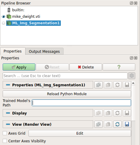
Plugin functionality. The plugins should allow the user to load the pre-trained models of their choice. This is achieved by enabling a text parameter in the Properties Panel of Paraview, that requires the path to the pre-trained model. The plugins can handle both absolute path as well as path relative to Paraview’s executable. The algorithm of the plugins then operate on the input data using the provided model. A screenshot of a plugin interface with the path parameter is provided in Figure 3 on the right-hand side.
Compatibility of VTK data models in plugins. According to the Paraview plugin mechanism [27], it is required to initially specify the VTK data models accepted for incoming input and outgoing output. However, the user may wish to apply a filter for a certain VTK data model that is different from the VTK data model the filter algorithm operates on. So, the idea of the plugins is that the core algorithm operates on only one VTK data model (which will be referred to as ’base VTK data model’) but is designed to accept multiple VTK data models as incoming input. The conversion from the other VTK data models to the base VTK data model is to be included internally in the plugin’s algorithm.

The general structure of the new data-driven filter plugins is given in Figure 4. Here, the major challenge is to appropriately map between the various data representations in VTK/Paraview and PyTorch.

The plugins are designed to feed data attributes of the VTK data models as input to pre-trained models. These data attributes are stored as VTK data arrays, however the pre-trained PyTorch model works with Tensor arrays as outlined in Section 3.4. So, a conversion between VTK data arrays and Tensor arrays is also required to couple the interface between Paraview and PyTorch. For this conversion, a NumPy interface is used in between due to the existing libraries offering conversion support between NumPy and VTK data arrays as well as NumPy and Tensor arrays. Thus, the conversion of Tensor to NumPy to VTK data arrays and vice-versa is performed with the modules: ’torch.from_numpy’, ’paraview.vtk.util.numpy_support’ and’vtkmodules.numpy_interface.dataset_adapter’.

The plugins use type checking in different steps to ensure a proper connection is established between different interfaces. This flow of data conversion is demonstrated with the generic plugin structure in Figure 4. Here, the accepted input VTK data models are A and B, where A is the base VTK data model, and the plugin supports conversion from data model B to A.

In Algorithm 1, we summarize the core functionality of the new filters for various input and output types, which will be further described in the next section. It is easy to observe that the previously described requirements on the plugin functionality and on the compatibility of the VTK data models are fulfilled.

Paraview plugins can be distributed in binary shared libraries or as a Python file. The Python-based plugins for this work have been developed with Paraview 5.8.1, PyTorch 1.6.0, NumPy 1.19.1 and Python 3.7.4.

At total of four plugins have been designed to show potential use cases of the Paraview-Pytorch coupling. All these plugins follow the same pipeline design mentioned before in Section 4.1, but the accepted input/output data models and the core algorithm of the filter varies. Two of the plugins provide filters for the task of segmentation and two of the plugins provide filters for the task of classification. For each task, we first have a prototypic filter, where we use image data as input and a pre-trained segmentation/classification model that is downloaded from PyTorch. While image data is certainly not the future intended input for a data-driven filter in Paraview, we use this test case as a sanity check and to shed light on the possibility to download and use pre-trained models in the context of Paraview. Similarly, for each task, we have as a second use case a fluid visualization oriented filter, which takes fluid data fields as input and provides a simplistic segmentation/classification example via a machine learning model trained by the authors (see Section 5). Overall, these use cases aim to show only simple prototypes of segmentation and classification within Paraview. In the future, more versatile machine learning models for e.g. turbulence classification or vortex region detection need to be developed. These can then be simply loaded into the already existing plugins.

This work uses DeepLab-v3 [8] as pre-trained model for image segmentation. The Deeplab-v3 model is a deep learning model built by Google with a ResNet-101 [34] backbone. It is trained on a subset of the COCO train2017 dataset with 21 labels and is available in a pre-trained form in PyTorch. [34, 8]

The used model requires the input of 3-channel (RBG) images normalized with the ImageNet [11] mean and standard deviation. The images need to be pre-processed to be in the right format for inference using the model. A forward pass through the model’s network results in 21 channels of output, and for each pixel, the index of the maximum output weight indicates its predicted class. The predicted class indices are then mapped to color values such that each class is represented by a different color.

One exemplary result of the developed image segmentation plugin is presented in Figure 5. The figure displays on the left-hand side the visualization view of an input image in Paraview with applied scalar mapping (defined in Section 3). On the right-hand side in the same figure, the output of the plugin using the DeepLab-v3 model is given. Obviously, the segmentation detects individually the bicycle and the background.

The architecture used to train the model for velocity segmentation is a simple neural network that contains 3 hidden linear layers with $80$, $40$ and $10$ neurons respectively and uses tanh as activation function. The input layer contains 3 neurons and the output layer contains 2 neurons. The training input is an array of size $2500$ with 3-component vector(velocity) values of a $50\times 50$ grid. The training output labels a point as 1 if the velocity magnitude in that point is greater than a specified value, referred to as threshold value, otherwise the point is labelled as 0. This classification is done for every point so the resulting grid gives a segmented grid, similar to a segmented image in Section 5.1. Obviously, the proposed segmentation is very similar to a data-driven replacement of the standard threshold filter provided by Paraview, hence it truly oversimplifies a segmentation for a velocity field. A more dedicated model would take the full velocity field as input and would e.g. characterize different parts of the field to be turbulent or laminar.

Our simplistic model was trained by the authors using the aforementioned neural network architecture with a threshold value $0.01$. The model was trained using the Cross Entropy Loss [17] and the Adam optimization algorithm [28] with a learning rate of $5\cdot 10^{-4}$. The dataset was divided such that $80\%$ of the dataset was used as training data and 20% as validation data, and the model was trained for 5000 epochs. The velocity data for training was taken from the mentioned lid-driven cavity flow simulation scene with Reynold’s number $10$, and strength of the inflow $2.0$ for $50\times 50$ grid. This data was generated from a simulation model based on Navier-Stokes equations [18], as outlined before. This simulation scene represents a highly viscous fluid.

An exemplary result of the Paraview filter plugin developed for velocity segmentation is presented in Figure 6, where the first one considers the velocity field for time step $t=0$ and the second one considers it for time step $t=20$. On the left-hand side of both figures, the input flow field is given. In the middle, the exact threshold segmentation is given, which we approximate by the segmentation model. On the right-hand side, the predicted threshold segmentation by our very simplistic model is provided.

The pre-trained image classification model Alexnet [29] is used for this application. Alexnet is a CNN architecture with 5 convolutional layers and 3 fully connected layers. Alexnet is provided with PyTorch pre-trained on the ImageNet [11] dataset with 1000 labels.

A forward pass through the model’s network results in 1000 channels of output, and the class with the maximum weight among the 1000 channels indicates its predicted class. The resulting weights are mapped into confidence scores of the model. The predicted classes and the confidence scores of the highest 10 scores are displayed in Spreadsheet View as a table in Paraview.

An exemplary result of the plugin developed for image classification is presented in Figure 7, with an input image visualized by Paraview with color mapping on the left-hand side and the Spreadsheet View of the output of the newly developed filter on the right-hand side.

The architecture used to train the model for pressure classification is a neural network that contains 2 hidden linear layers with $50$ and $20$ neurons and uses tanh as activation function. The input layer contains $2500$ neurons and the output layer contains 2 neurons. The training input is a flattened array of size $2500$ with scalar pressure values of a grid of size $50\times 50$. The training output is 1 if the maximum pressure value of the grid is greater than the threshold value, otherwise the output is 0. The weights of the two output neurons of the model are then transformed to be between the range of 0 and 1 using the Softmax function [17]. The index of the neuron with the highest transformed value indicates the predicted class. If the resulting index is 0, the class is labelled as ’Low’ and if the resulting index is 1, the class is labelled as ’High’. Certainly, this is again only a very simplistic classifier just designed for demonstration purposes.

A classification model was constructed by the authors using the aforementioned neural network architecture with a threshold value of $5.0$. The model was again trained over $500$ epochs using the Cross Entropy Loss and the Adam optimization algorithm with a learning rate of $5\cdot 10^{-4}$. $80\%$ of the underlying dataset was used as training data and 20% as validation data. The employed training data was again taken from the lid-driven cavity flow simulation scene with Reynold’s number $1000$, and inflow velocity $-1.0$ on a $50\times 50$ grid.

An exemplary result of the plugin developed for pressure classification is presented in Figure 8. It shows the input pressure field at time $t=5$ on the left hand-side and the plugin’s output in Spreadsheet View on the right-hand side.

References

- [1] J. Ahrens, B. Geveci, and C. Law. Paraview: An end-user tool for large-data visualization. In C. D. Hansen and C. R. Johnson, editors, Visualization Handbook, pages 717 – 731. Butterworth-Heinemann, Burlington, 2005.
- [2] G. Battineni, N. Chintalapudi, and F. Amenta. Machine learning in medicine: Performance calculation of dementia prediction by support vector machines (SVM). Informatics in Medicine Unlocked, Vol. 16:100200, 2019.
- [3] A. L. Beam and I. S. Kohane. Big Data and Machine Learning in Health Care. JAMA, Vol. 319(13):1317–1318, 2018.
- [4] E. Bertini and D. Lalanne. Surveying the complementary role of automatic data analysis and visualization in knowledge discovery. Proceedings of the ACM SIGKDD Workshop on Visual Analytics and Knowledge Discovery, VAKD ’09, 319(13):12–20, 01 2009.
- [5] M. Caron, P. Bojanowski, A. Joulin, and M. Douze. Deep clustering for unsupervised learning of visual features. In Computer Vision – ECCV 2018, pages 139–156. Springer International Publishing, 2018.
- [6] D. Chalupa and J. Mikulka. A novel tool for supervised segmentation using 3D slicer. Symmetry, Vol. 10:627, 2018.
- [7] S. Chauhan, K. Sell, W. Rühaak, T. Wille, and I. Sass. Cobweb 1.0: Machine learning tool box for tomographic imaging. Geoscientific Model Development, Vol. 13(1):315–334, 2020.
- [8] L.-C. Chen, G. Papandreou, F. Schroff, and H. Adam. Rethinking atrous convolution for semantic image segmentation, 2017.
- [9] X. Chen, Q. Guan, X. Liang, L.-T. Lo, S. Su, T. Estrada, and J. Ahrens. Tensorview: Visualizing the training of convolutional neural network using paraview. Proceedings of the 1st Workshop on Distributed Infrastructures for Deep Learning -DIDL, pages 11–16, 2017.
- [10] L. Codjo, M. Jaafar, H. Makich, D. Knittel, and M. Nouari. Honeycomb core milling diagnosis using machine learning in the industry 4.0 framework. 2018 IEEE 23rd International Conference on Emerging Technologies and Factory Automation (ETFA), Vol. 1:1251–1258, 2018.
- [11] J. Deng, W. Dong, R. Socher, L. Li, K. Li, and L. Fei-Fei. ImageNet: A large-scale hierarchical image database. 2009 IEEE Conference on Computer Vision and Pattern Recognition, pages 248–255, 2009.
- [12] T. G. Dietterich. Machine learning. ACM Computing Surveys, Vol. 28:3, 1996.
- [13] M. Everingham, L. Gool, C. K. I. Williams, J. Winn, and A. Zisserman. Pascal visual object classes challenge 2012 (VOC2012) complete dataset, 2012.
- [14] F.-Y. Tzeng and K.-L. Ma. Intelligent feature extraction and tracking for visualizing large-scale 4d flow simulations. In SC ’05: Proceedings of the 2005 ACM/IEEE Conference on Supercomputing, pages 6–6, 2005.
- [15] A. Fedorov, R. Beichel, J. Kalpathy-Cramer, J. Finet, J.-C. Fillion-Robin, S. Pujol, C. Bauer, D. Jennings, F. Fennessy, M. Sonka, J. Buatti, S. Aylward, J. V. Miller, S. Pieper, and R. Kikinis. 3D slicer as an image computing platform for the quantitative imaging network. Magnetic Resonance Imaging, Vol. 30(9):1323 – 1341, 2012.
- [16] A. Géron. Hands-on machine learning with Scikit-Learn, Keras, and TensorFlow: Concepts, tools, and techniques to build intelligent systems. O’Reilly Media, 2019.
- [17] I. Goodfellow, Y. Bengio, and A. Courville. Deep Learning. MIT Press, 2016.
- [18] M. Griebel, T. Dornseifer, and T. Neunhoeffer. Numerical Simulation in Fluid Dynamics. Society for Industrial and Applied Mathematics, 1998.
- [19] Y. Guo, T. T. Hormel, H. Xiong, J. Wang, T. S. Hwang, and Y. Jia. Automated segmentation of retinal fluid volumes from structural and angiographic optical coherence tomography using deep learning. Translational Vision Science & Technology, Vol. 9(2):54, 2020.
- [20] C. R. Harris, K. J. Millman, S. J. Walt, R. Gommers, P. Virtanen, D. Cournapeau, E. Wieser, J. Taylor, S. Berg, N. J. Smith, R. Kern, M. Picus, S. Hoyer, M. H. Kerkwijk, M. Brett, A. Haldane, J. F. Río, M. Wiebe, P. Peterson, P. Gérard-Marchant, K. Sheppard, T. Reddy, W. Weckesser, H. Abbasi, C. Gohlke, and T. E. Oliphant. Array programming with NumPy. Nature, 585(7825):357–362, 09 2020.
- [21] T. Hastie, R. Tibshirani, and J. Friedman. The elements of statistical learning: data mining, inference and prediction. Springer, 2nd edition, 2009.
- [22] H. Hauser and H. Schumann. Visualization Pipeline, pages 4553–4554. Springer New York, New York, NY, 2018.
- [23] K. He, X. Zhang, S. Ren, and J. Sun. Deep residual learning for image recognition. In IEEE Conference on Computer Vision and Pattern Recognition (CVPR), pages 770–778, 2016.
- [24] K. Inc. Color maps and transfer functions in paraview. https://docs.paraview.org/en/latest/ReferenceManual/colorMapping.html. Last access on 2021-04-27.
- [25] K. Inc. Data models in paraview. https://docs.paraview.org/en/latest/UsersGuide/understandingData.html. Last access on 2021-04-27.
- [26] K. Inc. vtktable class. https://vtk.org/doc/release/5.6/html/a01910.html. Last access on 2021-04-23.
- [27] K. Inc. Plugins in paraview. https://www.paraview.org/Wiki/ParaView/Plugin_HowTo, 1999. Last access on 2021-04-21.
- [28] D. Kingma and J. Ba. Adam: A method for stochastic optimization. arXiv preprint, abs/1412.6980, 2015.
- [29] A. Krizhevsky, I. Sutskever, and G. Hinton. Imagenet classification with deep convolutional neural networks. In F. Pereira, C. J. C. Burges, L. Bottou, and K. Q. Weinberger, editors, Advances in Neural Information Processing Systems, volume 25. Curran Associates, Inc., 2012.
- [30] A. Lasso, S. Alle, and Y.-T. Hsieh. 3D slicer plugin – NVIDIA AI Assisted Annotation Client. https://github.com/NVIDIA/ai-assisted-annotation-client/tree/master/slicer-plugin. Last access on 2020-11-24.
- [31] S. Leventhal, M. Kim, and D. Pugmire. Pave: An in situ framework for scientific visualization and machine learning coupling. In 2019 IEEE/ACM 5th International Workshop on Data Analysis and Reduction for Big Scientific Data (DRBSD-5), pages 8–15, 2019.
- [32] H. Li, S. Fang, S. Mukhopadhyay, A. Saykin, and L. Shen. Interactive machine learning by visualization: A small data solution. 2018 IEEE International Conference on Big Data (Big Data), pages 3513–3521, 2018.
- [33] D. Liu, W. Cui, K. Jin, Y. Guo, and H. Qu. Deeptracker: Visualizing the training process of convolutional neural networks. ACM Transactions on Intelligent Systems and Technology, Vol. 10(1), 2018.
- [34] J. Long, E. Shelhamer, and T. Darrell. Fully convolutional networks for semantic segmentation. In IEEE Conference on Computer Vision and Pattern Recognition (CVPR), pages 3431–3440, 2015.
- [35] K.-L. Ma. Machine learning to boost the next generation of visualization technology. IEEE Computer Graphics and Applications, Vol. 27(5):6–9, 2007.
- [36] D. Maharjan. GitHub project hosting plugins for data-driven filters in Paraview. https://github.com/drishti-m/Paraview_PyTorch_Plugin, 2021. Last access on 2021-04-21.
- [37] A. Paszke, S. Gross, F. Massa, A. Lerer, J. Bradbury, G. Chanan, T. Killeen, Z. Lin, N. Gimelshein, L. Antiga, A. Desmaison, A. Kopf, E. Yang, Z. DeVito, M. Raison, A. Tejani, S. Chilamkurthy, B. Steiner, L. Fang, J. Bai, and S. Chintala. PyiTorch: An imperative style, high-performance deep learning library. In H. Wallach, H. Larochelle, A. Beygelzimer, F. d'Alché-Buc, E. Fox, and R. Garnett, editors, Advances in Neural Information Processing Systems 32, pages 8024–8035. Curran Associates, Inc., 2019.
- [38] R. Peikert. Scientific Visualization, pages 3319–3320. Springer New York, New York, NY, 2018.
- [39] B. C. Russell, A. Torralba, K. P. Murphy, and W. T. Freeman. LabelMe: A database and web-based tool for image annotation. International Journal of Computer Vision, 77(1–3):157–173, May 2008.
- [40] W. Schroeder, K. Martin, and W. Lorensen. In The Visualization Toolkit, An Object-Oriented Approach To 3D Graphics, pages 161 – 178. Kitware, Inc., fourth edition, 2006.
- [41] V. Shrimali. A guide to workflow in PyTorch. https://learnopencv.com/pytorch-for-beginners-basics/. Last access on 2021-04-25.
- [42] W. Song, N. Zheng, R. Zheng, X.-B. Zhao, and A. Wang. Digital image semantic segmentation algorithms: A survey. Journal of Information Hiding and Multimedia Signal Processing, 10:196–211, 01 2019.
- [43] C. Szegedy, W. Liu, Y. Jia, P. Sermanet, S. Reed, D. Anguelov, D. Erhan, V. Vanhoucke, and A. Rabinovich. Going deeper with convolutions. IEEE Conference on Computer Vision and Pattern Recognition (CVPR), pages 1–9, 2015.
- [44] N. Thuerey, T. Kim, and T. Pfaff. Turbulent fluids. In ACM SIGGRAPH 2013 Courses, SIGGRAPH ’13, New York, NY, USA, 2013. Association for Computing Machinery.
- [45] D. A. Tillman, D. N. B. Duong, and N. S. Harding. Chapter 7 - modeling and fuel blending. In D. A. Tillman, D. N. B. Duong, and N. S. Harding, editors, Solid Fuel Blending, pages 271 – 293. Butterworth-Heinemann, Boston, 2012.
- [46] F.-Y. Tzeng, E. B. Lum, and K.-L. Ma. An intelligent system approach to higher dimensional classification of volume data. IEEE Transactions on Visualization and Computer Graphics, Vol. 11(3):273–284, 2005.
- [47] M. Watanabe, R. Kikinis, and C.-F. Westin. Level set-based integration of segmentation and computational fluid dynamics for flow correction in phase contrast angiography. Academic Radiology, Vol. 10(12):1416 – 1423, 2003.