Bayesian on-line anticipation of critical transitions
Zusammenfassung
The design of reliable indicators to anticipate critical transitions in complex systems is an important task in order to detect a coming sudden regime shift and to take action in order to either prevent it or mitigate its consequences. We present a data-driven method based on the estimation of a parameterized nonlinear stochastic differential equation that allows for a robust anticipation of critical transitions even in the presence of strong noise levels like they are present in many real world systems. Since the parameter estimation is done by a Markov Chain Monte Carlo approach we have access to credibility bands allowing for a better interpretation of the reliability of the results. By introducing a Bayesian linear segment fit it is possible to give an estimate for the time horizon in which the transition will probably occur based on the current state of information. This approach is also able to handle nonlinear time dependencies of the parameter controlling the transition. In general the method could be used as a tool for on-line analysis to detect changes in the resilience of the system and to provide information on the probability of the occurrence of a critical transition in future.
Keywords:
Anticipation of critical transitions Bayesian Modelling Leading Indicators Bifurcations Complex systemsIn complex systems in nature, technology and society smooth parameter changes can lead to sudden transitions between system states with very different behavior Scheffer 2009. Examples for such critical transitions occurring at tipping points are climate changes like desertification Corrado et al. 2014, greenhouse-icehouse transitions in the past Livina et al. 2010; Livina et al. 2013; Livina et al. 2015; Thompson and Sieber 2011; Lenton 2012, extinction of animal or bacteria species Veraart et al. 2011; Scheffer et al. 2009; Dakos et al. 2008; Dakos and Bascompte 2014; Dakos et al. 2017, allograft rejection Izrailtyan et al. 2000, chronic diseases Rikkert et al. 2016, power outages Cotilla-Sanchez et al. 2012; Ren and Watts 2015, the Laser threshold and the onset of convection Haken 2004, transitions in human movement Haken et al. 1985 and much more Strogatz 2015; Jurczyk et al. 2017; van de Leemput et al. 2013; Chadefaux 2014; Gopalakrishnan et al. 2016; Lim and Epureanu 2011. Sometimes, these transitions have severe consequences Boers and Rypdal 2021; Klose et al. 2020; Ritchie et al. 2021; Lohmann and Ditlevsen 2021; Lenton et al. 2019 and it would be important to find methods to anticipate critical transitions and strategies to prevent or avoid damage Batt et al. 2019; Hagstrom and Levin 2017; Ewel et al. 2001.
In many natural systems where critical transitions occur, the detailed mechanisms are barely understood. Nevertheless, it is well known that in many cases complex systems composed out of a large number of nonlinear interacting parts can be described by only a few macroscopic degrees of freedom if they are close to a critical transition Haken 2004. The critical transition of the complex system connected to a smooth parameter change corresponds to a bifurcation of the evolution equation. This bifurcation induced scenario is sometimes called B-tipping Ritchie and Sieber 2017; Ashwin et al. 2012. Since these bifurcation scenarios are rather universal one can expect that for a large class of systems, like the examples mentioned above, a coming bifurcation can be anticipated by observing universal indicators that are correlated to the loss of linear stability or by directly observing an estimate of a numerical linear stability analysis.
So in recent years a plenty of time series analysis methods based on the assumption of universal indicators have been developed to solve the problem of anticipating a coming bifurcation Dakos et al. 2012; Dakos et al. 2009; Liang et al. 2017; Scheffer et al. 2015. A non-parametric ansatz is implemented in Carpenter and Brock 2011; Anvari et al. 2016 in which the estimation of a drift-diffusion-jump model is suggested in case of high-frequency time series. The most simple leading indicators to anticipate a critical transition are the autocorrelation at lag-1 combined with the standard deviation based on the phenomenon of critical slowing down prior to a bifurcation scenario, the kurtosis based on the changing shape of the underlying potential and the skewness based on flickering in noisy systems Scheffer et al. 2012; qiang Xie et al. 2018. The measures are evaluated in rolling windows and need a preparation of the data, e.g. detrending in each window. They are loosely connected to the mathematical description of complex systems and their positive trends are sometimes misleading or difficult to interpret, because of missing uncertainty estimates and sometimes autocorrelation and standard deviation do not increase at the same time as they should if they are candidates for an uprising transition Boerlijst et al. 2013; Gsell et al. 2016; Ditlevsen and Johnsen 2010. In general, the briefly mentioned stability measures and leading indicators suffer from their difficult interpretation due to noisy trends and missing uncertainty estimates. Besides, selecting historical test data based on the knowledge that those datasets exhibit a transition can lead to statistical mistakes in the leading indicators’ performance and quality Boettiger and Hastings 2012. Furthermore, they are rather susceptible for artefacts that are not related to critical transitions, but caused by a changing variance, sub-optimal detrending of the time series or simply preprocessing issues Wilkat et al. 2019; Clements et al. 2015; Hastings and Wysham 2010; Perretti and Munch 2012; Dablander et al. 2020. Additionally, high noise levels can have strong negative influence on the performance of leading indicators Perretti and Munch 2012. Another important issue is the estimation of the point in time at which the transition will probably take place. Even in cases where a reliable leading indicator can be computed it is still difficult to give an estimate for the time horizon in which the transition will occur. Though it is possible to extrapolate a straight line based on the most current calculated leading indicator values, this strategy will fail to give an reliable estimate in more complicated situations, e.g. the onset of a parameter trend of unknown shape out of a regime with a constant control parameter.
In the following we will develop a method to anticipate critical transitions in complex systems which solves many of the shortcomings of the aforementioned approaches. The method is based on the assumption that the measured time series can be modeled by a nonlinear stochastic differential equation (SDE). Therefore, the parameters of the model can be linked directly to linear stability analysis and the inclusion of higher order terms in the ansatz for the SDE allows for a reliable statement about the stability of the system even in the presence of strong noise. The parameters’ estimation is done in a Bayesian way providing access to the complete posterior distribution of the parameters and subsequently allowing for the specification of credibility intervals. To estimate the beginning of the transition towards a different regime and the time horizon in which the transition can be expected we introduce a Bayesian non-parametric linear segment fit von der Linden et al. 2014; Dose and Menzel 2004 which is able to react to sudden changes of the control parameter trend under rather simple assumptions.
The paper is divided into three parts. In section I the model assumptions and the estimation procedure are introduced. In section II the method is applied as an example to two synthetic models and a statistical comparison to the above mentioned leading indicators autocorrelation, standard deviation, kurtosis and skewness is given. The method is also applied to a non-Markovian dataset to get an impression of the reliability under imperfect circumstances and the non-parametric linear segment fit approach is presented as an example. At last, a short summary and conclusion is presented in section III.
I Developing the method
I.1 The model approach for the observed data
The system under consideration is assumed to be relaxed onto a stable fixed point. It explores the phase space close to the fixed point due to noise and as a result one observes a fluctuating time series of the system. The starting hypothesis is similar to the ansatz in Carpenter and Brock 2011 and assumes that the observed signal can be described by a SDE of the Langevin Kloeden and Platen 1992 form
| (1) |
where is the nonlinear deterministic part, the so-called drift, and is the diffusion term. The noise is assumed to be Gaussian and -correlated. For the remainder of the article we assume that we can make the approximation that the noise strength does not significantly depend on the state an we can set .
The loss of stability of the fixed point followed by a bifurcation is described by the change of the sign of the slope
| (2) |
of the nonlinear drift at the fixed point . Since we assume to be in a fixed point and close to a bifurcation we develop into a Taylor series up to order three which is sufficient to describe the normal forms of simple bifurcation scenarios Strogatz 2015. This results in
| (3) |
so that the information on the linear stability is incorporated in . For practical reasons equation 3 is used in the form
| (4) |
in the numerical approach, where an arbitrary fixed point is incorporated in the coefficients by algebraic transformation and comparison of coefficients. The polynomial model up to order three is denoted as , a simple linear model is called . Now, the time series can be divided into short windows where the parameters can be assumed to be nearly constant. Estimating the parameters within the windows and observing their change from window to window give us information on the evolution of the stability of the system in time. Since one is interested only in the change of the slope at the fixed point one could restrict this ansatz to the first order term . But if the noise is strong enough to drive the system away from the fixed point, like it is assumed to be e.g. in ecological systems Perretti and Munch 2012, contributions of the higher order terms may become significant and their incorporation leads to a much more reliable estimation of the slope . Additionally, close to the bifurcation the nonlinear terms play a more significant role since the first order term goes to zero which is the reason for critical slowing down and critical fluctuations.
I.2 Bayesian estimation of the model parameters
We have to estimate the model parameters from the data to observe the change of the stability within the moving windows. Here we choose a Bayesian approach since this allows for the computation of the full posterior distribution of the parameters via Markov Chain Monte Carlo (MCMC) and a consistent inclusion of prior information von der Linden et al. 2014. Using Bayes’ theorem the posterior distribution of the parameters is defined as
| (5) |
with the evidence , which normalizes the posterior distribution, the likelihood and the prior distribution . The posterior allows for the consistent definition of credibility intervals of the estimated parameters. The likelihood relates the measured data to the underlying model and is given by the transition probability of the Markov process defined by (1). The transition probability for subsequent times and with which is also denoted as short time propagator Risken 1996 is defined as
| (6) |
The priors are generally chosen in a broad range to allow for the determination of the parameters due to the available data instead of strong prior assumptions. For the linear parts of the deterministic functions and the uninformative Jeffreys’ prior von der Linden et al. 2014
| (7) |
is chosen. It is improper in the constant , but that does not matter for parameter estimation. The scale variable is modelled by Jeffreys’ scale prior von der Linden et al. 2014
| (8) |
These choices simulate best the real situation in which no or just poor prior information is available. Furthermore, it is taken care that the parameters of the higher orders are initially able to contribute in a similar magnitude to the deterministic dynamics as the linear ones by wide Gaussian priors
| (9) | ||||
centred around the mean with standard deviations in an adequate range.
The posterior can be computed approximately by hand for the simple linear approximation . The detailed solution involves the assumption of a Gaussian posterior, the use of perturbation theory and a Taylor expansion. It can be found in von der Linden et al. 2014. However, the posterior distribution for more complicated models as the third order polynom cannot be computed analytically, but by using a MCMC approach. Here we use an affine-invariant ensemble sampler with a so-called stretch step. It implements an ensemble of Markov chains at the same time. The proposal for the Markov chain is drawn from a proposal distribution that is based on the current states of the complementary ensemble . This shortens the integrated autocorrelation length and improves the computational performance. We use the version implemented in the python package emcee Foreman-Mackey et al. 2013.
Based on the posterior distribution we can compute the posterior pdfs of the slope by marginalization. The posterior pdf of the slope of the linear model is easily accessible via
| (10) |
and the posterior pdf of the slope of the third order drift model is given by
| (11) |
Now we can define the credibility intervals as the to - and to -percentiles of the corresponding pdf. It is computed from a kernel density estimate of the corresponding pdf Pedregosa et al. 2011.
I.3 Bayesian estimation of change points
By using the method described in the last section we can reliably estimate the parameters of the model (1) in a moving window. By observing the change of from window to window we can detect the change in the degree of stability or more generally, the resilience Scheffer et al. 2018 of the system, and can decide whether the system drifts towards an upcoming critical transition. Nevertheless, the method has to be extended to tackle two additional questions. In many situations the system is in stable operation and at a certain point in time it starts to change its stability for example due to the change of external conditions. Observing the fluctuations of the frequency in a power grid to anticipate an outage would be an example for this situation Cotilla-Sanchez et al. 2012. In this cases it would be important, e.g. for an on-line warning system, to detect the point where the system starts loosing its stability as soon as possible. The second point is the question at which time the transition will occur. In principle, the question can be answered by extrapolating the indicator values computed in the time windows by a straight line to find the point in time where the indicator crosses the critical value. Nevertheless, this approach is obviously not very reliable. To solve the two problems we extend the method by including a non-parametric Bayesian linear segment fit into our method. Such a fitting approach is even able to be adapted in an on-line application and provides forecasts for possible critical transitions with corresponding uncertainties based on the current information. In general, the method assumes that the dataset can be fitted by a predefined number of linear segments divided by so-called change points where the segments can change their slope. In case of one change point the dataset is fitted by two linear segments with different slopes connected at the change point. In our application the dataset is the set of slope indicator values . If we assume change points we have linear segments
| (12) |
for and the change point vector with the entries for , whereby denotes the data size and the vector contains the design ordinates at the assumed change point positions. Now, the goal is to calculate the probability
| (13) |
that a certain configuration of change points is realised in the dataset . The dataset is expanded by each step of the moving window approach. Furthermore, we assume that the system initially is in a steady state and that the slope calculated in the moving window fluctuates around a fixed value. In this case there is no change point within the actual dataset and the result is a flat distribution (13). If time proceeds a control parameter starts to change and causes the stability of the system to degrade. In consequence the slope indicator will start to change and (13) will be peaked around a certain which can then be identified as pint where the system starts to change its stability. In consequence, the data will be fitted by a nearly constant segment and a segment with finite slope beginning at the change point and we are able to detect the beginning destabilizing process. Given this information we can forecast the point where crosses zero by computing the sum of the forecasts gained from all possible change point configurations weighted with their posterior probabilities. In the case of only one change point this would correspond to a simple straight line extrapolation of the data. However, it is not guaranteed that the time evolution of the control parameter is linear. The approach can be extended in a straightforward way to deal with a nonlinear dependence of the control parameter by introducing additional change points in the fit. This becomes more and more computational expensive so we restrict the ansatz in this paper to two change points. The details to calculate the posterior (13) and the forecast can be found in von der Linden et al. 2014; Dose and Menzel 2004.
Given the procedure above, the approach is able to react to sudden changes of the trend of the control parameter and enables us to extrapolate the trend based on the available data to find possible transition times including their uncertainty based on the model assumptions. The results of the described slope estimation procedure and an exemplary discussion of the Bayesian non-parametric transition anticipation method are presented in the following section II.
II Numerical results
In subsection II.1 the Bayesian stability estimation approach is tested against two simulated datasets of which one passes through a fold and the other through a pitchfork bifurcation. A comparison to known leading indicator candidates is given in subsection II.2. Moreover, the method is applied to a non-Markovian dataset in II.3 to provide an example for the robustness of the evaluation under imperfect conditions.
Finally, in subsection II.4 the before mentioned non-parametric linear segment fit is applied as an example to a fold bifurcation model.
II.1 Bayesian case studies with simulated data
The method is tested on two simple synthetic datasets of which one is given by a SDE with
| (14) | |||
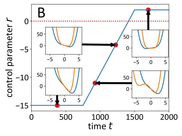
where is the control parameter. The simulation is performed with the Euler-Maruyama scheme Kloeden and Platen 1992; Bronstein et al. 2008 for SDEs. The time range is set to . The simulation is performed for a linearly increasing control parameter from to . In consequence, the critical transition due to a fold bifurcation is expected around . One realisation with data points and a noise level of is shown in subfigure 1 that gives an impression of the numerical estimation procedure. The control parameter , shown in 1, is fixed at for the first data points, before it increases linearly up to at time where it is fixed again for data points. The analysis is done on rolling time windows of size as suggested by the green area in 1.
Starting with this time series the Bayesian analysis approach is applied to each window in order to get insights in the stability and model parameters of the system. The prior range is chosen adequately wide by the interval for and for the stochastic constant factor to guarantee the determination of the posterior distribution by the available data instead of the prior assumptions. The standard deviations of the Gaussian priors for are chosen to be , respectively. In each window the parameters of the third order model are estimated as the maximum posterior solutions of the corresponding pdfs. The posterior pdfs for the rolling time window ending at time are illustratively shown in the subfigures 1, 1 and 1.These pdfs can be helpful to identify the role of the model parameters: Most of the probability density mass of the parameter suggests , whereas the pdfs of the parameters and are more defined around zero and could be less significant for the model at hand. The quadratic term is not as defined as the latter two what means a considerable probability for . The noise level pdf includes the real value of that is marked by the green vertical dotted line. The question is: Do the estimated parameters provide an approximately realistic impression of the dynamical situation? In order to answer this question the true potential and the potential that is estimated via the maximum posterior solutions of the parameters are shown as blue and orange lines, respectively, in the sub-windows of subfigure 1 at the exemplary time and , and . The blue signed original potential tilts over from the stable fixed point to a new stable position . The estimated orange potential preserves the main features of the original potential and follows the same tilting behaviour for increasing . Generally, it is estimated too narrow as expected due to the limited information that is provided by the time series data in terms of the noise that explores the corresponding phase space. In conclusion, the illustration shows that the estimates are reasonable and can be used to calculate the drift slope that contains information about the stability and upcoming transitions in the system dynamics. The pdf and its evolution over time is resolved in 1. The pdfs at time and are in the initial fixed regime and approximately equal as expected. When the parameter starts its linear upwards trend the slope pdfs approach zero and thus, indicate less stable states and indirectly a parameter change in . Note, that the width of the posterior pdfs decrease strongly in the vicinity of the critical transition. This could mean that the data are more informative in its vicinity.



Thus, the tipping point is correctly indicated by the trend of the MCMC estimate of the drift slope . Figure 2 shows the time evolution of the maximum posterior slope estimates including the corresponding credibility intervals for the standard deviations , and of the noise. The results estimated with the linear model and the polynom model for small and moderate noise contributions as and are almost the same. Therefore, only the polynom estimates are shown in 2 and 2. Only around the actual bifurcation point the results differ slightly, i.d. the linear order model saturates at instead of the threshold crossing seen for the polynom model . The difference in the precision and trend quality is evident for higher noise influence as compared in subfigure 2: The linear model cannot resolve the critical threshold crossing at the bifurcation point whereas the polynom model is able to handle the noisy situation. Note, that for moderate noise like the scenario investigated in subfigure 2 the slope estimates do not reach the critical threshold, but contain a small jump. In contrast to the scenario with there is no pronounced flickering and the phase space is not explored by a sufficient noise level to anticipate the critical transition exactly.


The investigations are proceeded by applying the Bayesian leading indicator approach to another model in order to control its robustness regarding bifurcation types and systems. To this end, a simple model that exhibits a pitchfork bifurcation is computed via a SDE with
| (15) | ||||
with the control parameter that changes linearly in time from to during the simulation with the Euler-Maruyama scheme. The parameters are chosen analogously to the fold model parameters in 2. The two valleys of the underlying double well potential converge to the unstable branch due to the linear shift in and a single stable branch around zero remains for . The method is tested against this model for different noise levels of which the cases with standard deviation , and are shown in this paper. An exemplary dataset with is presented in figure 4. The orange branches indicate stable fixed point positions and the orange dotted horizontal line an unstable fixed point of the typical pitchfork. The data follows the upper branch up to the time signed by the blue dotted vertical line where flickering occurs. The noise level lies widely in the flickering regime that starts around in the simulations’ setup. The simulated datasets with standard deviation and follow a similar behaviour but do not show pronounced flickering near the critical threshold that is reached at the red dotted vertical line. The Bayesian stability analysis approach turns out to be able to anticipate the ongoing destabilization processes in the pitchfork datasets. The linear as well as the polynom model, and , respectively, yield very similar results for the smaller noise cases as presented in the subfigures 2 and 2. For that reason only the polynom estimations are shown. The advantage of the polynom model lies again in the better handling of highly noisy situations as visible in 2. Of course, the flickering caused by the high noise is not anticipated by none of the estimators. There is a jump in the indicator trend when the flickering starts around the blue dotted vertical line. Nevertheless, the flickering regime up to the critical transition at the critical threshold is reproduced rather correctly by the slope estimates with the polynom estimator , whereas the linear estimator does not cross the stability threshold zero.
The robustness against high noise is a big problem of known leading indicator candidates. To this end, the performance of the introduced slope estimate and already known leading indicator candidates is compared in the following subsection II.2.


II.2 Robustness against noise
In many real world applications an analyst has to deal with highly noisy measurement environments. Therefore, the ability of a leading indicator candidate to provide reliable anticipation results is considered in a comparative way: The commonly discussed indicators autocorrelation at lag-1 (AR1), standard deviation (std ), skewness and kurtosis are compared with the introduced drift slope indicator for the fold model of equation 14 in a wide range of noise levels , , , , , and . Thus, the noise performance scan incorporates lots higher noise levels than the proposed real noise level of an ecological system around Perretti and Munch 2012. Nevertheless, a highly resolved time series and the gradient of a shifting control parameter remain important restrictions to apply the above mentioned indicators successfully.
In order to avoid the influence of the window size in a dynamic approach and to include a comprehensive set of noise realisations the procedure is as follows: First, 240 time series of data points are simulated over the time interval for each investigated noise level each of which with an equidistantly changed control parameter over the range . This avoids the influence of rolling window size and dynamic changes taking place in a finite window. Second, the test set of leading indicators is applied to the time series generated that way over the whole data points to incorporate the noise dynamics. In that way, 240 leading indicator results depending on the control parameter are computed for each noise level and truncated at the time where . Third, these indicator series are checked with a Bayesian model comparison von der Linden et al. 2014 whether they exhibit a linear gradient (model 1 ) or are just constant (model 2 ). The computed Bayes factors () are defined as the fraction of the model evidences where indicates the evidence of over . The Bayes factors are calculated with a standard Gaussian prior for the intercept with means defined by the first data value . A uniform prior in the range or for some decreasing skewness cases is chosen for the slope, respectively, and the noise is included with a uniform noise prior in the range . The convergence of the MC evaluations is guaranteed by draws of prior models in each Bayes factor calculation.
The results are summarized in table 1. A Bayes factor is assumed to be a significant sign of preferring to or vice versa. Following this threshold clearly pronounced gradients are highlighted in green, clearly identified constants in orange and insignificant values in grey in table 1. The slope indicator exhibits significant positive trends in a realistic and wide range of noise levels , whereas the often mentioned AR1 and std are not as reliable as one may expect. The AR1 is significant only in the small noise regime and sensitive to high time series resolutions. A too narrow sampling causes a high autocorrelation at lag-1 and thus, weakens the overall trend. This could be avoided by lower sampling or calculation of autocorrelation at a higher time lag. The std is only significant for and sensitive to a low resolution of the time series. The skewness provides good performance results in the high noise regime without any exception. For smaller noise levels the skewness is insignificant because of the absence of flickering. The kurtosis has a very bad performance regarding the Bayes factor results. For low noise levels it is insignificant, for a noise around positive and for all tested higher noise cases it is described by a constant model which would erroneously indicate no transition.
II.3 Non-Markovian data
Up to now the noise is assumed to be Gaussian and -correlated in time so that the process obeys the Markov properties Kloeden and Platen 1992; Klöckner et al. 2014. But it is emphasized that empirical tests suggest that even if the Markov assumption is not fulfilled - i.e. the data is simulated with correlated noise and thus, non-Markovian - the trend of the stability indicator remains the same apart from some shift in its absolute values as discussed in the example in this section. Thus, its interpretation is not necessarily strongly affected.
The basic assumption of a Markovian process is not necessarily fulfilled in realistic scenarios. Nevertheless, the heuristic ansatz of the method that is introduced in the paper, does not loose its principal validity: In figure 4 the method is applied to a realisation of a non-Markovian Risken 1996 fold model, i.e.
| (16) | |||
with the parameters , , and a control parameter linearly increasing in the range . The slope estimates are computed with the method and a polynomial model with constant noise level . The illustration 4 suggests the general validity of the method and its ability to determine destabilizing trends even in non-Markovian time series data, whereas the absolute values are affected by a value shift.
The case studies on the fold and pitchfork model are completed at this point. In the following subsection II.4 the idea of providing a transition time estimate with uncertainty bands is proposed.
II.4 Non-parametric anticipation of critical transitions
The problem of forecasting possible transition times in a reliable manner remains unsolved so far, but the non-parametric fit approach explained in detail in von der Linden et al. 2014; Dose and Menzel 2004 is a useful tool to face the problem. To this end the proposed transition time estimation approach is presented as an example on the slope estimates of the fold dataset that is presented above in 1. This data exhibits a constant control parameter up to time and then starts to shift linearly up to at time . In this paper the on-line application is simulated by successively updating the available slope estimates and repeating the Bayesian fit process in each step. For practical reasons the fitting procedure is started under the assumption of one possible change point. The uprising control parameter trend is detected and well fitted at . After identification of a change point a second possible change point is incorporated in the assumptions to take care of possibly further changing parameter trends. Thus, the assumption of two change points is included for times . Snapshots of the extrapolation method are shown in figure 6. The red dotted vertical line marks the time at which the control parameter crosses its critical value. The blue dotted vertical line indicates the actual critical transition defined analogously to subfigure 1. For the problem at hand it is also reasonable to choose -credibility intervals for the fit functions to be also aware of critical transitions that could occur much earlier than the most probable transition. In subfigures 6 and 6 the control parameter is constant. In both situations no critical transition is anticipated in the near future. Nevertheless, the very small amount of data and the assumption of a possible change point in the segment fit leads to a wide uncertainty range in 6, that even proposes a small possibility for a transition in the shown interval of the investigated time series. As the available data of the constant stable regime increases the uncertainty decreases as visible in 6. The segment fit detects the uprising destabilization process very precisely as underlined by 6. The change point is correctly detected and the extrapolation predicts the correct interval for an uprising transition based on the currently available data around time points before it occurs. Also in the subfigures 6 to 6 the uncertainty range covers the correct interval.
The forecast transition times as well as their upper and lower bounds are considered in a statistical analysis over the time interval in order to


get an idea of the reliability of the predictions in that model case. The results are summarized in figure 6. The probability distributions contain the right transition interval, whereas their maxima are behind the actual transition time. This is an expected result because of the rolling time window method that incorporates a delayed trend in the drift slope calculations. Nevertheless, the distributions give an idea of the probability of a critical transition for different times in future. After the time of the performed fits suggest the actual transition prior to time and even of the individual fits contain the right transition time in their corresponding confidence bands.
III Conclusion and outlook
In this paper we have introduced a robust method to anticipate critical transitions due to bifurcations and applied it to a system with a fold and a pitchfork bifurcation. The method is based on the hypothesis that the measured data can be described by a parametric nonlinear SDE. The estimation of the coefficients of the SDE allows for a direct access to the linear stability of the system via the slope of the deterministic part of the SDE at the fixed point. By including nonlinear terms into the ansatz the method provides reliable response to destabilization even in the presence of strong noise. Thanks to the Bayesian approach of parameter estimation we have full access to the posterior pdfs of the parameters via MCMC and can consistently define credibility intervals which are important for the interpretation of the results. The upper uncertainty bound of the slope of the SDE’s deterministic part yields a reliable limit for the earliest possible transition time with respect to the actual transition time of the two investigated simple models. The inclusion of a Bayesian non-parametric linear segment fit allows for both an on-line determination of change points in the current trend and the estimation of the point where the transition probably will take place in the future based on the current information.
The forecast procedure can also be adapted to nonlinear time evolution of the control parameter by introducing more change points. Nevertheless, this increases the computational costs of the method which might be problematic for on-line applications. Therefore, further work has to be done to make the method also feasible for on-line applications with nonlinear trends towards tipping points.
Data availability
The datasets as well as the simulations and analyis codes are available upon request from the authors under a CC BY-NC-ND 4.0 International license.
Acknowledgements
We thank colleagues and friends for proofreading the manuscript. M. H. thanks the Studienstiftung des deutschen Volkes for a scholarship including financial support.
Literatur
- Scheffer (2009) M. Scheffer, Critical Transitions in Nature and Society , paperback ed. (Princeton University Press, 2009) p. 400.
- Corrado et al. (2014) R. Corrado, A. M. Cherubini, and C. Pennetta, Early warning signals of desertification transitions in semiarid ecosystems, Physical Review E 90, 10.1103/physreve.90.062705 (2014).
- Livina et al. (2010) V. N. Livina, F. Kwasniok, and T. M. Lenton, Potential analysis reveals changing number of climate states during the last 60 kyr, Climate of the Past 6, 77 (2010).
- Livina et al. (2013) V. Livina, G. Lohmann, M. Mudelsee, and T. Lenton, Forecasting the underlying potential governing the time series of a dynamical system, Physica A: Statistical Mechanics and its Applications 392, 3891 (2013).
- Livina et al. (2015) V. N. Livina, T. M. V. Martins, and A. B. Forbes, Tipping point analysis of atmospheric oxygen concentration, Chaos: An Interdisciplinary Journal of Nonlinear Science 25, 036403 (2015).
- Thompson and Sieber (2011) J. M. T. Thompson and J. Sieber, Predicting climate tipping as a noisy bifurcation: A review, International Journal of Bifurcation and Chaos 21, 399 (2011).
- Lenton (2012) T. M. Lenton, Arctic climate tipping points, AMBIO 41, 10 (2012).
- Veraart et al. (2011) A. J. Veraart, E. J. Faassen, V. Dakos, E. H. van Nes, M. Lurling, and M. Scheffer, Recovery rates reflect distance to a tipping point in a living system, Nature 481, 357 (2011).
- Scheffer et al. (2009) M. Scheffer, J. Bascompte, W. A. Brock, V. Brovkin, S. R. Carpenter, V. Dakos, H. Held, E. H. van Nes, M. Rietkerk, and G. Sugihara, Early-warning signals for critical transitions, Nature 461, 53 (2009).
- Dakos et al. (2008) V. Dakos, M. Scheffer, E. H. van Nes, V. Brovkin, V. Petoukhov, and H. Held, Slowing down as an early warning signal for abrupt climate change, Proceedings of the National Academy of Sciences 105, 14308 (2008), http://www.pnas.org/content/105/38/14308.full.pdf .
- Dakos and Bascompte (2014) V. Dakos and J. Bascompte, Critical slowing down as early warning for the onset of collapse in mutualistic communities, Proceedings of the National Academy of Sciences 111, 17546 (2014).
- Dakos et al. (2017) V. Dakos, S. M. Glaser, C. hao Hsieh, and G. Sugihara, Elevated nonlinearity as an indicator of shifts in the dynamics of populations under stress, Journal of The Royal Society Interface 14, 20160845 (2017).
- Izrailtyan et al. (2000) I. Izrailtyan, J. Kresh, R. J. Morris, S. C. Brozena, S. P. Kutalek, and A. S. Wechsler, Early detection of acute allograft rejection by linear and nonlinear analysis of heart rate variability, The Journal of Thoracic and Cardiovascular Surgery 120, 737 (2000).
- Rikkert et al. (2016) M. G. M. O. Rikkert, V. Dakos, T. G. Buchman, R. de Boer, L. Glass, A. O. J. Cramer, S. Levin, E. van Nes, G. Sugihara, M. D. Ferrari, E. A. Tolner, I. van de Leemput, J. Lagro, R. Melis, and M. Scheffer, Slowing down of recovery as generic risk marker for acute severity transitions in chronic diseases, Critical Care Medicine 44, 601 (2016).
- Cotilla-Sanchez et al. (2012) E. Cotilla-Sanchez, P. D. H. Hines, and C. M. Danforth, Predicting critical transitions from time series synchrophasor data, IEEE Transactions on Smart Grid 3, 1832 (2012).
- Ren and Watts (2015) H. Ren and D. Watts, Early warning signals for critical transitions in power systems, Electric Power Systems Research 124, 173 (2015).
- Haken (2004) H. Haken, Synergetics (Springer Berlin Heidelberg, 2004).
- Haken et al. (1985) H. Haken, J. A. S. Kelso, and H. Bunz, A theoretical model of phase transitions in human hand movements, Biological Cybernetics 51, 347 (1985).
- Strogatz (2015) S. H. Strogatz, Nonlinear dynamics and chaos. With Applications to Physics, Biology, Chemistry and Engineering., second edition ed. (Westview Press, 2015).
- Jurczyk et al. (2017) J. Jurczyk, T. Rehberg, A. Eckrot, and I. Morgenstern, Measuring critical transitions in financial markets, Scientific Reports 7, 10.1038/s41598-017-11854-1 (2017).
- van de Leemput et al. (2013) I. A. van de Leemput, M. Wichers, A. O. J. Cramer, D. Borsboom, F. Tuerlinckx, P. Kuppens, E. H. van Nes, W. Viechtbauer, E. J. Giltay, S. H. Aggen, C. Derom, N. Jacobs, K. S. Kendler, H. L. J. van der Maas, M. C. Neale, F. Peeters, E. Thiery, P. Zachar, and M. Scheffer, Critical slowing down as early warning for the onset and termination of depression, Proceedings of the National Academy of Sciences 111, 87 (2013).
- Chadefaux (2014) T. Chadefaux, Early warning signals for war in the news, Journal of Peace Research 51, 5 (2014).
- Gopalakrishnan et al. (2016) E. A. Gopalakrishnan, Y. Sharma, T. John, P. S. Dutta, and R. I. Sujith, Early warning signals for critical transitions in a thermoacoustic system, Scientific Reports 6, 10.1038/srep35310 (2016).
- Lim and Epureanu (2011) J. Lim and B. I. Epureanu, Forecasting a class of bifurcations: Theory and experiment, Physical Review E 83, 10.1103/physreve.83.016203 (2011).
- Boers and Rypdal (2021) N. Boers and M. Rypdal, Critical slowing down suggests that the western greenland ice sheet is close to a tipping point, Proceedings of the National Academy of Sciences 118, e2024192118 (2021).
- Klose et al. (2020) A. K. Klose, V. Karle, R. Winkelmann, and J. F. Donges, Emergence of cascading dynamics in interacting tipping elements of ecology and climate, Royal Society Open Science 7, 200599 (2020).
- Ritchie et al. (2021) P. D. L. Ritchie, J. J. Clarke, P. M. Cox, and C. Huntingford, Overshooting tipping point thresholds in a changing climate, Nature 592, 517 (2021).
- Lohmann and Ditlevsen (2021) J. Lohmann and P. D. Ditlevsen, Risk of tipping the overturning circulation due to increasing rates of ice melt, Proceedings of the National Academy of Sciences 118, e2017989118 (2021).
- Lenton et al. (2019) T. M. Lenton, J. Rockström, O. Gaffney, S. Rahmstorf, K. Richardson, W. Steffen, and H. J. Schellnhuber, Climate tipping points — too risky to bet against, Nature 575, 592 (2019).
- Batt et al. (2019) R. D. Batt, T. Eason, and A. Garmestani, Time scale of resilience loss: Implications for managing critical transitions in water quality, PLOS ONE 14, e0223366 (2019).
- Hagstrom and Levin (2017) G. I. Hagstrom and S. A. Levin, Marine ecosystems as complex adaptive systems: Emergent patterns, critical transitions, and public goods, Ecosystems 20, 458 (2017).
- Ewel et al. (2001) K. C. Ewel, C. Cressa, R. T. Kneib, P. S. Lake, L. A. Levin, M. A. Palmer, P. Snelgrove, and D. H. Wall, Managing critical transition zones, Ecosystems 4, 452 (2001).
- Ritchie and Sieber (2017) P. Ritchie and J. Sieber, Probability of noise- and rate-induced tipping, Physical Review E 95, 10.1103/physreve.95.052209 (2017).
- Ashwin et al. (2012) P. Ashwin, S. Wieczorek, R. Vitolo, and P. Cox, Tipping points in open systems: bifurcation, noise-induced and rate-dependent examples in the climate system, Philosophical Transactions of the Royal Society A: Mathematical, Physical and Engineering Sciences 370, 1166 (2012).
- Dakos et al. (2012) V. Dakos, S. R. Carpenter, W. A. Brock, A. M. Ellison, V. Guttal, A. R. Ives, S. Kéfi, V. Livina, D. A. Seekell, E. H. van Nes, and M. Scheffer, Methods for detecting early warnings of critical transitions in time series illustrated using simulated ecological data, PLoS ONE 7, e41010 (2012).
- Dakos et al. (2009) V. Dakos, E. H. van Nes, R. Donangelo, H. Fort, and M. Scheffer, Spatial correlation as leading indicator of catastrophic shifts, Theoretical Ecology 3, 163 (2009).
- Liang et al. (2017) J. Liang, Y. Hu, G. Chen, and T. Zhou, A universal indicator of critical state transitions in noisy complex networked systems, Scientific Reports 7, 10.1038/srep42857 (2017).
- Scheffer et al. (2015) M. Scheffer, S. R. Carpenter, V. Dakos, and E. H. van Nes, Generic indicators of ecological resilience: Inferring the chance of a critical transition, Annual Review of Ecology, Evolution, and Systematics 46, 145 (2015).
- Carpenter and Brock (2011) S. R. Carpenter and W. A. Brock, Early warnings of unknown nonlinear shifts: a nonparametric approach, Ecology 92, 2196 (2011).
- Anvari et al. (2016) M. Anvari, M. R. R. Tabar, J. Peinke, and K. Lehnertz, Disentangling the stochastic behavior of complex time series, Scientific Reports 6, 10.1038/srep35435 (2016).
- Scheffer et al. (2012)
M. Scheffer, S. R. Carpenter, T. M. Lenton, J. Bascompte,
W. Brock, V. Dakos, J. van de Koppel, I. A. van de Leemput, S. A. Levin, E. H. van Nes, M. Pascual, and J. Vandermeer, Anticipating critical transitions, Science 338, 344 (2012), http://science.sciencemag.org/content/338/6105/
344.full.pdf . - qiang Xie et al. (2018) X. qiang Xie, W. ping He, B. Gu, Y. Mei, and S. shan Zhao, Can kurtosis be an early warning signal for abrupt climate change?, Climate Dynamics 52, 6863 (2018).
- Boerlijst et al. (2013) M. C. Boerlijst, T. Oudman, and A. M. de Roos, Catastrophic collapse can occur without early warning: Examples of silent catastrophes in structured ecological models, PLoS ONE 8, e62033 (2013).
- Gsell et al. (2016) A. S. Gsell, U. Scharfenberger, D. Özkundakci, A. Walters, L.-A. Hansson, A. B. G. Janssen, P. Nõges, P. C. Reid, D. E. Schindler, E. V. Donk, V. Dakos, and R. Adrian, Evaluating early-warning indicators of critical transitions in natural aquatic ecosystems, Proceedings of the National Academy of Sciences 113, E8089 (2016).
- Ditlevsen and Johnsen (2010) P. D. Ditlevsen and S. J. Johnsen, Tipping points: Early warning and wishful thinking, Geophysical Research Letters 37, n/a (2010).
- Boettiger and Hastings (2012) C. Boettiger and A. Hastings, Early warning signals and the prosecutor's fallacy, Proceedings of the Royal Society B: Biological Sciences 279, 4734 (2012).
- Wilkat et al. (2019) T. Wilkat, T. Rings, and K. Lehnertz, No evidence for critical slowing down prior to human epileptic seizures, Chaos: An Interdisciplinary Journal of Nonlinear Science 29, 091104 (2019).
- Clements et al. (2015) C. F. Clements, J. M. Drake, J. I. Griffiths, and A. Ozgul, Factors influencing the detectability of early warning signals of population collapse, The American Naturalist 186, 50 (2015).
- Hastings and Wysham (2010) A. Hastings and D. B. Wysham, Regime shifts in ecological systems can occur with no warning, Ecology Letters 13, 464 (2010).
- Perretti and Munch (2012) C. T. Perretti and S. B. Munch, Regime shift indicators fail under noise levels commonly observed in ecological systems, Ecological Applications 22, 1772 (2012).
- Dablander et al. (2020) F. Dablander, A. Pichler, A. Cika, and A. Bacilieri, Anticipating critical transitions in psychological systems using early warning signals: Theoretical and practical considerations, PsyArXiv 10.31234/osf.io/5wc28 (2020).
- von der Linden et al. (2014) W. von der Linden, V. Dose, and U. von Tussaint, Bayesian Probability Theory. Applications in the Physical Sciences (Cambridge University Press, 2014).
- Dose and Menzel (2004) V. Dose and A. Menzel, Bayesian analysis of climate change impacts in phenology, Global Change Biology 10, 259 (2004).
- Kloeden and Platen (1992) P. E. Kloeden and E. Platen, Numerical Solution of Stochastic Differential Equations (Springer Berlin Heidelberg, 1992).
- Risken (1996) H. Risken, The Fokker-Planck Equation: Methods of Solutions and Applications (Springer Series in Synergetics), 2nd ed. (Springer, 1996).
- Foreman-Mackey et al. (2013) D. Foreman-Mackey, D. W. Hogg, D. Lang, and J. Goodman, emcee: The MCMC hammer, Publications of the Astronomical Society of the Pacific 125, 306 (2013).
- Pedregosa et al. (2011) F. Pedregosa, G. Varoquaux, A. Gramfort, V. Michel, B. Thirion, O. Grisel, M. Blondel, P. Prettenhofer, R. Weiss, V. Dubourg, J. Vanderplas, A. Passos, D. Cournapeau, M. Brucher, M. Perrot, and Édouard Duchesnay, Scikit-learn: Machine learning in python, Journal of Machine Learning Research 12, 2825 (2011).
- Scheffer et al. (2018) M. Scheffer, J. E. Bolhuis, D. Borsboom, T. G. Buchman, S. M. W. Gijzel, D. Goulson, J. E. Kammenga, B. Kemp, I. A. van de Leemput, S. Levin, C. M. Martin, R. J. F. Melis, E. H. van Nes, L. M. Romero, and M. G. M. O. Rikkert, Quantifying resilience of humans and other animals, Proceedings of the National Academy of Sciences 115, 11883 (2018).
- Bronstein et al. (2008) I. N. Bronstein, K. A. Semendjajew, G. Musiol, and H. Mühlig, Taschenbuch der Mathematik, 7th ed. (Harri Deutsch, Frankfurt a. M., 2008).
- Klöckner et al. (2014) A. Klöckner, F. van der Linden, and D. Zimmer, Noise generation for continuous system simulation, in Proceedings of the 10th International Modelica Conference, March 10-12, 2014, Lund, Sweden (Linköping University Electronic Press, 2014).