\jdate

March 2003 \pagerangeStable Marriage Problems with Ties and Incomplete Preferences: An Empirical Comparison of ASP, SAT, ILP, CP, and Local Search Methods–References

Stable Marriage Problems with Ties and Incomplete Preferences: An Empirical Comparison of ASP, SAT, ILP, CP, and Local Search MethodsDOI: S1471068401001193

SELIN EYUPOGLU¹ MUGE FIDAN¹ YAVUZ GULESEN¹ ILAYDA BEGUM IZCI¹ BERKAN TEBER¹ BATURAY YILMAZ¹ AHMET ALKAN² ESRA ERDEM¹
¹ Computer Science Faculty of Engineering and Natural Sciences Sabanci University Istanbul Turkey
² Economics Faculty of Arts and Social Sciences Sabanci University Istanbul Turkey

2003

Abstract

We study a variation of the Stable Marriage problem, where every man and every woman express their preferences as preference lists which may be incomplete and contain ties. This problem is called the Stable Marriage problem with Ties and Incomplete preferences (SMTI). We consider three optimization variants of SMTI, Max Cardinality, Sex-Equal and Egalitarian, and empirically compare the following methods to solve them: Answer Set Programming, Constraint Programming, Integer Linear Programming. For Max Cardinality, we compare these methods with Local Search methods as well. We also empirically compare Answer Set Programming with Propositional Satisfiability, for SMTI instances. This paper is under consideration for acceptance in Theory and Practice of Logic Programming (TPLP).

keywords

stable marriage problems, declarative problem solving, answer set programming, propositional satisfiability, integer linear programming, constraint programming, local search

1 Introduction

Matching problems have been studied in economics, starting with the seminal paper of \citeNgale1962college, which has led to a Nobel Prize in 2012, utilizing game theory methods with the goal of a mechanism design. Matching problems are about markets where individuals are matched with individuals, firms, or items, typically across two sides, as in employment [39] (e.g., who works at which job), kidney donation (e.g., who receives which transplantable organ) [33, 38], and marriages [24, 14] (e.g., who marries with whom). In each problem, preferences of individuals, firms, or items are given, possibly along with other information (e.g., the quotas of the universities in university entrance) [2, 1].

One of the well-known matching problems is the Stable Marriage Problem (SM). In SM, for a set of $n$ men and $n$ women, we are given the preferences of individuals: for each man, a complete ranking of the women is specified as preferred partners; similarly, for each woman, a complete ranking of the men is specified as preferred partners. The goal is to marry all men and women (i.e., to find $n$ couples) in such a way that marriages are stable: no man and woman in different couples prefer each other to their partners.

We consider a variant of SM, called SMTI, where rankings may be incomplete (i.e., some partners are not acceptable) or may include ties (i.e., some partners are preferred equally). We investigate three hard variants of SMTI [28, 32], that aim to compute optimal stable matchings with respect to different measures of fairness: sex-equality (preferences of men and women are considered to be equally important), egalitarian (preferences of every individual are considered to be equally important), maximum cardinality (minimizes the number of singles).

We present a variety of methods to solve these problems, using Answer Set Programming (ASP) [34, 36, 29, 41, 5], Integer Linear Programming (ILP) [27], Constraint Programming (CP) [25, 42, 37], and Local Search (including Hill-Climbing [31, 40] and Genetic Algorithms [22]).

The ASP formulations of SMTI and its hard variants (Sex-Equal SMTI, Egalitarian SMTI, Max Cardinality SMTI) are novel (Section 3); they are implemented for the ASP solver Clingo [15]. We consider the ILP formulation of Max Cardinality SMTI, by Delorme et al. Delorme et al. 2019 as a basis, and introduce the ILP formulations for Sex-Equal SMTI and Egalitarian SMTI (Section 4); they are implemented for Gurobi and Google-OR Tools (MIP and CP). We consider the local search algorithms introduced by Gelain et al. Gelain et al. 2013 and Haas et al. Haas 2020 for Max Cardinality SMTI (Section 5), and implement them with slight variations. We compare these methods empirically over a large set of randomly generated instances (Section 6).

We also compare ASP with propositional satisfiability (SAT) Gomes et al. 2007; Biere et al. 2009 over randomly generated SMTI instances. For a comparison of ASP with SAT, we adapt the ASP implementation of SMTI for Cmodels Giunchiglia et al. 2004 that utilizes the SAT solver ZChaff Moskewicz et al. 2001 to compute solutions. We also adapt the SAT formulation of SMTI by Drummond et al. 2015 (SAT-E) to include ties, and use the SAT solver Lingeling Biere 2010 to compute solutions.

The implementations and the benchmarks are available at https://github.com/KRR-SU/SMTI-TPLP-2021.

2 The Stable Marriage Problems with Ties and Incomplete Lists (SMTI)

The Stable Marriage problem with Ties and Incomplete lists (SMTI) is defined by a set $M$ of men, a set $W$ of women, for each man $x\in M$ a partial ordering $\succ_{x}$ over $W_{x}\subseteq W$ , and for each woman $y\in W$ a partial ordering $\succ_{y}$ over $M_{y}\subseteq M$ .

Let $\hbox{\it mrank\/}:M\times W\mapsto\{1,\dots,|W|\}$ be a partial function such that $\hbox{\it mrank\/}(x,y)=r$ represents that a woman $y$ is man $x$ ’s $r$ th preferred choice with respect to $\succ_{x}$ and $\hbox{\it wrank\/}:W\times M\mapsto\{1,\dots,|M|\}$ be a partial function such that $\hbox{\it wrank\/}(y,x)=r$ represents that a man $x$ is woman $y$ ’s $r$ th preferred choice with respect to $\succ_{y}$ .

A man $x$ is acceptable to a woman $y$ if $\hbox{\it wrank\/}(x,y)$ is defined. Similarly, a woman $y$ is acceptable for a man $x$ if $\hbox{\it mrank\/}(x,y)$ is defined.

A matching for a given SMTI instance is a partial function $\mu:M\mapsto W$ . A man $x$ is single if $\mu(x)$ is undefined and a woman $y$ is single if $\mu^{-1}(y)$ is undefined.

A pair $(x,y)$ of a man and a woman is called a blocking pair for a matching $\mu$ if the following conditions hold:

A1

$x$ and $y$ are acceptable to each other,
A2

$x$ and $y$ are not married to each other (i.e., $\mu(x)\neq y$ ),
A3
- (a)
  
  $x$ and $y$ are both single,
- (b)
  
  $\hbox{\it mrank\/}(x,y)<\hbox{\it mrank\/}(x,\mu(x))$ and $y$ is single,
- (c)
  
  $\hbox{\it wrank\/}(y,x)<\hbox{\it wrank\/}(y,\mu^{-1}(y))$ and $x$ is single or
- (d)
  
  $\hbox{\it mrank\/}(x,y)<\hbox{\it mrank\/}(x,\mu(x))$ and $\hbox{\it wrank\/}(y,x)<\hbox{\it wrank\/}(y,\mu^{-1}(y))$ .

A matching for SMTI is called stable if it is not blocked by any pair of agents. Note that we consider weakly stable matchings. It is assumed that marriage to an acceptable partner is preferred over being single.

We consider three hard variants of SMTI Kato 1993; Manlove et al. 2002, that aim to compute optimal stable matchings with respect to different measures of fairness: sex-equality, egalitarian and maximum cardinality.

Egalitarian SMTI.

Egalitarian SMTI maximizes the total satisfaction of the preferences of all agents. Since the preferred agents have lower rankings, this total satisfaction is maximized when the sum of ranks of all agents is minimized.

Let $\mu$ be a matching and $\mathcal{M}$ denote the set of matchings in a given problem. For every man $x\in M$ , we define the satisfaction $c_{\mu}(x)$ of $x$ ’s preferences with respect to $\mu$ as follows: $c_{\mu}(x){=}R$ if $\hbox{\it mrank\/}(x,\mu(x)){=}R$ . Similarly, for every woman $y\in W$ , we define the satisfaction $c_{\mu}(y){=}R$ if $\hbox{\it wrank\/}(y,\mu^{-1}(y)){=}R$ . Then, the total satisfaction of preferences of all agents is defined as follows: $c(\mu)=\sum_{x\in M\cup W}c_{\mu}(x).$ Then, a matching $\mu{\in}\mathcal{M}$ with the minimum $c(\mu)$ is egalitarian.

Sex-Equal SMTI.

Sex-Equal SMTI maximizes the equality of satisfaction among sexes. We define the sex equality by the following cost function $c(\mu){=}|\sum_{x\in M}c_{\mu}(x)-\sum_{y\in W}c_{\mu}(y)|.$ Then, a matching $\mu{\in}\mathcal{M}$ with the minimum $c(\mu)$ is sex-equal.

Max Cardinality SMTI.

Max Cardinality SMTI maximizes the number of matched pairs. A matching $\mu{\in}\mathcal{M}$ is a maximum cardinality matching if it is a matching that maximizes $|\mu|$ . The number of matched pairs is maximized when the number of singles is minimized.

3 Solving SMTI Problems using ASP and SAT

We formalize input of an SMTI instance $\langle M,W,\hbox{\it mrank\/},\hbox{\it wrank\/}\rangle$ in ASP by a set $F_{I}$ of facts using atoms of the forms $\hbox{\it man\/}(x)$ (“ $x$ is a man in $M$ ”), $\hbox{\it woman\/}(y)$ (“ $y$ is a woman in $W$ ”), $\hbox{\it mrank\/}(x,y,r)$ (i.e., $\hbox{\it mrank\/}(x,y)=r$ ) and $\hbox{\it wrank\/}(y,x,r)$ (i.e., $\hbox{\it wrank\/}(y,x)=r$ ). In the ASP formulation $P$ of SMTI, the variables $x$ , $x1$ denote men in $M$ and $y$ , $y1$ denote women in $W$ .

The first pair of rules of the program $P$ characterize a set of individuals of the opposite set for each man and woman who they prefer over being single:

\begin{array}[]{l}\hbox{\it maccept\/}(x,y)\leftarrow\hbox{\it mrank\/}(x,y,r).\\ \hbox{\it waccept\/}(y,x)\leftarrow\hbox{\it wrank\/}(y,x,r).\\ \end{array}

and the concept of mutual acceptability:

\begin{array}[]{l}\hbox{\it acceptable\/}(x,y)\leftarrow\hbox{\it maccept\/}(x,y),\hbox{\it waccept\/}(y,x).\end{array}

We define preferences of man $x$ (i.e., $x$ prefers $y$ to $y1$ ) and woman $y$ (i.e., $y$ prefers $x$ to $x1$ ) in terms of rankings.

\begin{array}[]{l}\hbox{\it mprefer\/}(x,y,y1)\leftarrow\hbox{\it mrank\/}(x,y1,r),\hbox{\it mrank\/}(x,y,r1),r>r1.\\ \hbox{\it wprefer\/}(y,x,x1)\leftarrow\hbox{\it wrank\/}(y,x1,r),\hbox{\it wrank\/}(y,x,r1),r>r1.\\ \end{array}

We define a matching between men and women where both parties find each other acceptable with the cardinal constraint of 1 for each man.

\begin{array}[]{l}$\lx@text@lbrace$\hbox{\it marry\/}(x,y):\hbox{\it acceptable\/}(x,y)$\lx@text@rbrace 1$\leftarrow\hbox{\it man\/}(x).\\ \end{array}

In order to guarantee that a woman is not matched to more than one man, we use the following constraint:

\begin{array}[]{l}\leftarrow$\lx@text@lbrace$\hbox{\it marry\/}(x,y):\hbox{\it man\/}(x)$\lx@text@rbrace$>1,\hbox{\it woman\/}(y).\end{array}

Individuals who stay single under the represented matching by marry atoms are described by the msingle and wsingle atoms.

\begin{array}[]{l}\hbox{\it msingle\/}(x)\leftarrow\hbox{\it man\/}(x),$\lx@text@lbrace$\hbox{\it marry\/}(x,y):\hbox{\it woman\/}(y)$\lx@text@rbrace 0$.\\ \hbox{\it wsingle\/}(y)\leftarrow\hbox{\it woman\/}(y),$\lx@text@lbrace$\hbox{\it marry\/}(x,y):\hbox{\it man\/}(x)$\lx@text@rbrace 0.$\end{array}

To establish stability, we refer to conditions A1–A3. The following set of constraints respectively describe and eliminate blocking pairs that are described by (a) – (d) of A3. Conditions A1 and A2 also hold for each constraint.

\begin{array}[]{l}\leftarrow\hbox{\it acceptable\/}(x,y),\hbox{\it msingle\/}(x),\hbox{\it wsingle\/}(y).\\ \leftarrow\hbox{\it wsingle\/}(y),\hbox{\it marry\/}(x,y1),\hbox{\it mprefer\/}(x,y,y1),\hbox{\it acceptable\/}(x,y).\\ \leftarrow\hbox{\it msingle\/}(x),\hbox{\it marry\/}(x1,y),\hbox{\it wprefer\/}(y,x,x1),\hbox{\it acceptable\/}(x,y).\\ \leftarrow\hbox{\it marry\/}(x,y1),\hbox{\it marry\/}(x1,y),\hbox{\it mprefer\/}(x,y,y1),\hbox{\it wprefer\/}(y,x,x1).\\ \end{array}

Given the ASP formulation $P$ whose rules are described above and the ASP description $F_{I}$ of an SMTI instance $I$ , the ASP solver Clingo generates a stable matching.

We can transform the ASP program $P\cup F_{I}$ into an equivalent propositional theory $\Gamma(I)$ so that the answer sets for $P\cup F_{I}$ and the models for $\Gamma(I)$ are in a 1-1 correspondence Erdem and Lifschitz 2003; Lin and Zhao 2004. The ASP solver Cmodels Giunchiglia et al. 2004 is developed on this idea, and thus allows us to utilize SAT solvers (e.g., ZChaff Moskewicz et al. 2001) to compute solutions for SMTI instances. An alternative SAT encoding of SMTI can be obtained from the formulation of Drummond et al. 2015.

To solve Sex-Equal SMTI, we add the following weak constraint to optimize sex equality:

\begin{array}[]{l}\xleftarrow{\backsim}t=\#\hbox{\it sum\/}\{r1-r2,x,y:\hbox{\it marry\/}(x,y),\hbox{\it mrank\/}(x,y,r1),\hbox{\it wrank\/}(y,x,r2)\}.\ [|t|@1]\end{array}

To solve Egalitarian SMTI, we add the following weak constraint to minimize the cost function:

\begin{array}[]{l}\xleftarrow{\backsim}\hbox{\it marry\/}(x,y),\hbox{\it mrank\/}(x,y,r1),\hbox{\it wrank\/}(y,x,r2).\ [r1+r2@1]\end{array}

To solve Max Cardinality SMTI, we add the following weak constraints to minimize the number of singles:

\begin{array}[]{l}\xleftarrow{\backsim}\hbox{\it wsingle\/}(x).\ [1@1,W,x]\\ \xleftarrow{\backsim}\hbox{\it msingle\/}(y).\ [1@1,M,y]\\ \end{array}

Note that combinations of these optimizations are possible, by giving priorities to weak constraints: instead of specifying just the weight $t$ of the weak constraints, we need to specify also their priorities $p$ by an expression $w@p$ . The weak constraints are supported by the ASP solver Clingo but not by Cmodels.

4 Solving SMTI using ILP and CP

We consider the ILP formulation of Max Cardinality SMTI by Delorme et al. Delorme et al. 2019 as a basis and introduce ILP formulations for Sex-Equal SMTI and Egalitarian SMTI.

Let us introduce the necessary notation to describe the ILP formulation.

•

$ML$ : A list of lists of size $n$ . $ML[i]$ represents a preference list of man $i$ .
•

$WL$ : A list of lists of size $n$ . $WL[j]$ represents a preference list of woman $j$ .
•

$ML_{{i}_{\leq}}(j)$ : Set of men that woman $j$ ranks at the same level or better than man $i$ .
•

$WL_{j_{\leq}}(i)$ : Set of women that man $i$ ranks at the same level or better than woman $j$ .
•

$mrank(i,j)$ : The rank of woman $j$ in $ML[i]$ .
•

$wrank(j,i)$ : The rank of man $i$ in $WL[j]$ .
•

$M$ : A matrix of size $n\times n$ which denotes the matching where rows represent men and columns represent women.
•

$x_{ij}$ : A binary variable that refers to an index of $M$ , and is equal to 1 if man $i$ and woman $j$ are matched, 0 otherwise.

The acceptability constraint forces the variable $x_{ij}$ to be 0 if man $i$ and woman $j$ are not mutually acceptable:

\begin{array}[]{l}$$\{x_{ij}=0:i\notin WL[j],j\notin ML[i]\}.$$\end{array}

The following constraint ensures that each man is matched to at most one woman. Since at most one $x_{ij}$ value can be equal to 1, sum of the cells in a row $i$ of $M$ should be at most one:

\begin{array}[]{l}$$\sum_{j\in WL}x_{ij}\leq 1.$$\end{array}

Similarly, the following constraint ensures each woman is matched to at most one man:

\begin{array}[]{l}$$\sum_{i\in ML}x_{ij}\leq 1.$$\end{array}

The stability constraint ensures that there are no blocking pairs. The variable $q$ in the following constraint represents a member of the set of women who has the same or better rank than woman $j$ for a man $i$ , and $p$ represents a member of the set of men who has the same or better rank than man $i$ for woman $j$ . Hence, if man $i$ is matched to someone who is not $q$ , or woman $j$ is matched to someone who is not $p$ , man $i$ and woman $j$ form a blocking pair:

\begin{array}[]{l}$$1-\sum_{q\in WL_{{j}_{\leq}}(i)}x_{iq}\leq\sum_{p\in ML_{{i}_{\leq}}(j)}x_{pj}.$$\end{array}

The following objective function represents the Max Cardinality optimization for the ILP model:

\max(\sum_{i\in ML}\sum_{j\in WL}x_{ij}).

Since the matrix $M$ denotes the matching and every matrix cell, denoted by variable $x_{ij}$ , is 1 when the pair represented with that cell is matched; maximizing the sum of all cells corresponds to maximizing the number of matched pairs.

We use the following objective function for Sex-Equal optimization:

\min(|\sum_{i\in ML}\sum_{j\in WL}(mrank(i,j)\times x_{ij}-wrank(j,i)\times x_{ij})|).

This objective function aims to minimize the difference between the sum of the ranks of matched pairs from men’s perspective and the sum of the ranks of matched pairs from women’s perspective.

The following objective function provides Egalitarian optimization:

\min(\sum_{i\in ML}\sum_{j\in WL}(mrank(i,j)\times x_{ij}+wrank(j,i)\times x_{ij})).

In Egalitarian optimization, the total satisfaction of individuals is maximized. Since better preference yields lower rank, by minimizing sum of ranks of all matched pairs, the total satisfaction is maximized.

We implement the ILP models using Gurobi and Google OR-Tools MIP. With slight variations of the Google-OR Tools MIP implementation, we can also utilize Google-OR Tools CP.

5 Solving Max Cardinality SMTI using Local Search Algorithms

To compare with the ASP, ILP and CP approaches to solve Max Cardinality SMTI, we also consider the existing local search algorithms.

Random-Restart Stochastic Hill-Climbing Search.

We consider the local search algorithm LTIU introduced by Gelain et al. Gelain et al. 2013 to solve Max Cardinality SMTI as the basis. The input of this algorithm consists of the sets of $n$ men and $n$ women, preference lists of each man and woman, and a step or a time limit $T$ .

LTIU performs a random-restart stochastic hill-climbing search (Algorithm 1). The local search starts from a random matching. The neighbors of a matching $\mu$ are all matchings obtained from $\mu$ by removing one ‘‘undominated’’ blocking pair.¹¹ 1 Given two blocking pairs $(m,w)$ and $(m,w^{\prime})$ , $(m,w)$ dominates (from the men’s point of view) $(m,w^{\prime})$ if $m$ prefers $w$ to $w^{\prime}$ . It is also defined for the women’s point of view. A men- (resp., women-) undominated blocking pair is a blocking pair such that there is no other blocking pair that dominates it from the men’s (resp., women’s) point of view. The objective function is the sum of the number of blocking pairs and the number of singles.

LTIU tries to minimize the value of this objective function: at each search step, it chooses a random matching that has the minimum evaluation value. If there exists no matching such that its evaluation value is less than the current matching, then the algorithm chooses a random matching from the neighborhood. Furthermore, with a certain probability, LTIU can choose a random matching in the neighborhood.

The algorithm terminates when it finds a perfect matching (i.e., a matching with no singles and no blocking pairs) or it reaches the time limit. If the algorithm does not find any stable matching during the search, then the best matching with a minimum evaluation value is returned.

During the search, a random restart is applied in order to avoid search near local minima (i.e., it reaches a matching with no blocking pair and thus, has an empty neighborhood).

Genetic Algorithm.

We consider the genetic algorithm (GA) introduced by Haas 2020 to solve Max Cardinality SMTI (Algorithm 2). Unlike other methods, the algorithm generates stable pairs at every step to obtain matchings with improved properties.

According to the GA approach, chromosomes are solutions to the given SMTI problem. In other words, a chromosome is a stable matching $\langle X,Y\rangle$ containing several genes which are pairs of matched women and men $\langle x_{i},y_{i}\rangle$ . To create stable chromosomes for the initial population, ties are arbitrarily broken, then the Gale-Shapley algorithm, also known as deferred acceptance algorithm (DA), is used to find stable matchings.

The fitness function is constructed based on the optimization variant. For Max Cardinality SMTI, a chromosome/matching $\mu$ is said to be fitter if the property $NumPairs=\sum_{\langle x,y\rangle}\{\langle x,y\rangle|x\neq\emptyset\land y\neq\emptyset\}$ is higher for that matching.

To improve the fitness of the chromosome/matching to the desired outcome, two genetic operators are used: the cycle crossover operator and the mutation operator. The fittest individuals are chosen randomly at each iteration to mate and bear offspring. Initially, individuals are randomly selected based on their ranks. The formula for calculating the chance to select an individual (for population $P$ and individual $i$ ) is as follows:

chance(i)=\frac{fitness(i)}{\sum_{k\in P}fitness(k)}.

By integrating two parents’ solutions, the cycle crossover operator produces new possible solutions by selecting a sequence of two or more pairs and flips either $x$ or $y$ for each pair in the sequence.

The mutation operator searches for Pareto-improvement cycles as described by Erdil and Ergin 2008 to increase the number of matched participants, provided a certain mutation probability.

Our implementation of GA concentrates solely on stable allocations for the Two-Sided Matching application. Particularly, as part of crossover and mutation operators, we have included additional controls that define possible blocking pairs introduced by the changes and only consider adjustments to be acceptable if they do not lead to blocking pairs to ensure that the genetic algorithm returns valid and stable allocations Haas 2020.

6 Experiments

We have empirically compared different methods to solve SMTI and its hard variants.

Experimental Setup.

To test and analyze the models and our implementations, we need an instance generator. For this, we have implemented the random instance generator proposed by Gent and Prosser 2002.

The random instance generator takes 3 inputs to generate instances: instance size $n$ , (i.e, number of men and women), probability of incompleteness $p1$ , and probability of ties $p2$ . We have generated a benchmark set, with instance sizes $n=50$ and $n=100$ , where the value of $p1$ changes in the range of [0.1, 0.8] and the value of $p2$ changes in the range [0.1, 0.9] with 0.1 step. There are 144 combinations and for each combination, we have generated 10 instances and averaged the results.

The tests were run on a local machine which has Ubuntu 18.04.1 as operating system and x86_64 processor. The algorithms are implemented in Python programming language with version 3.6.9. Additionally, we use Gurobi version 9.1.1, OR-Tools version 8.1.8487, Clingo version 5.2.2, Cmodels version 3.79 with the SAT solver ZChaff 2007.3.12, and SAT-E version released on May 17, 2016 with the SAT solver Lingeling bcj.

We set the time limit for each solver to 2000 seconds, memory limit to 2 GB, and step limits for LTIU and GA implementations to 50000, and 10000, respectively. In GA experiments, the population size is set to 50, the number of evolution rounds is set to 1000, and the mutation probability is set to $0.2$ . In LTIU experiments, we set the probability of selecting a random matching from the neighborhood to $0.2$ .

Table 1: SMTI: Average CPU-Times (in seconds) for varying

p1

and

p2

values with

n=50

Solver	$p1$	0.1	0.2	0.3	0.4	0.5	0.6	0.7	0.8	0.9
		$p2$
Clingo	0.1	5.07	4.99	4.96	4.82	4.74	4.61	4.36	4.03	3.09
	0.2	3.41	3.39	3.33	3.27	3.17	3.04	2.91	2.63	1.88
	0.3	2.11	2.05	2.02	2.01	1.92	1.86	1.73	1.51	1.14
	0.4	1.23	1.2	1.17	1.19	1.12	1.09	1.0	0.92	0.63
	0.5	0.68	0.65	0.65	0.64	0.61	0.6	0.51	0.45	0.34
	0.6	0.35	0.33	0.35	0.32	0.3	0.29	0.26	0.22	0.17
	0.7	0.16	0.15	0.15	0.14	0.14	0.14	0.12	0.11	0.09
	0.8	0.06	0.07	0.06	0.06	0.07	0.06	0.05	0.05	0.03
Cmodels	0.1	7.29	7.18	7.18	6.93	6.62	6.44	5.97	5.41	4.38
	0.2	4.92	4.95	4.85	4.7	4.6	4.2	4.04	3.7	2.95
	0.3	3.34	3.31	3.23	3.17	3.03	3.01	2.68	2.41	1.88
	0.4	2.02	1.99	1.97	1.98	1.89	1.83	1.64	1.53	1.11
	0.5	1.19	1.12	1.16	1.13	1.06	1.07	0.89	0.81	0.61
	0.6	0.61	0.57	0.6	0.56	0.51	0.5	0.46	0.39	0.28
	0.7	0.26	0.25	0.24	0.23	0.23	0.22	0.19	0.17	0.13
	0.8	0.1	0.1	0.1	0.09	0.1	0.09	0.08	0.08	0.07
SAT-E	0.1	0.79	0.84	0.86	0.88	0.93	0.94	0.98	0.98	1.0
	0.2	0.62	0.67	0.68	0.7	0.74	0.78	0.78	0.84	0.82
	0.3	0.51	0.54	0.55	0.58	0.6	0.65	0.66	0.68	0.69
	0.4	0.4	0.41	0.42	0.44	0.46	0.48	0.5	0.53	0.56
	0.5	0.31	0.32	0.33	0.34	0.35	0.36	0.36	0.39	0.4
	0.6	0.24	0.25	0.26	0.26	0.27	0.28	0.28	0.28	0.29
	0.7	0.18	0.18	0.18	0.19	0.19	0.2	0.2	0.2	0.2
	0.8	0.13	0.13	0.13	0.14	0.14	0.15	0.14	0.15	0.15

Table 2: SMTI: Average CPU-Times (in seconds) for varying

p1

and

p2

values with

n=100

Solver	$p1$	0.1	0.2	0.3	0.4	0.5	0.6	0.7	0.8	0.9
		$p2$
Clingo	0.1	120.5	116.94	122.21	121.05	107.89	108.29	104.07	95.7	81.07
	0.2	80.14	80.63	78.42	79.3	74.38	69.78	68.89	66.07	54.74
	0.3	45.37	45.36	43.66	43.22	40.64	38.17	39.63	34.1	29.4
	0.4	27.52	26.65	26.15	25.84	25.27	23.86	22.75	21.76	17.96
	0.5	14.52	14.06	14.13	13.99	13.93	13.13	13.29	11.21	9.64
	0.6	7.12	7.16	7.2	7.02	6.87	7.53	6.17	5.83	4.63
	0.7	3.12	3.19	3.12	3.12	3.08	3.09	2.8	2.41	1.87
	0.8	0.95	0.96	0.97	0.92	0.93	0.84	0.74	0.64	0.46
Cmodels	0.1	M	M	M	M	M	M	M	M	M
	0.2	M	M	M	M	M	M	M	M	M
	0.3	M	M	M	M	M	M	M	M	M
	0.4	M	M	M	M	M	M	M	M	M
	0.5	23.29	23.33	23.49	23.66	23.91	23.77	21.38	17.03	14.37
	0.6	12.63	12.93	12.97	12.62	11.95	11.72	10.22	8.64	6.71
	0.7	4.62	4.85	4.66	4.73	4.87	4.62	3.88	3.44	2.71
	0.8	1.47	1.42	1.45	1.4	1.4	1.28	1.16	1.01	0.76
SAT-E	0.1	6.04	5.78	6.79	6.84	6.96	7.48	8.0	7.24	5.99
	0.2	4.91	4.92	5.02	5.98	5.73	5.82	6.57	7.68	4.69
	0.3	3.87	3.98	4.67	4.54	5.09	4.09	4.02	4.83	4.07
	0.4	2.74	3.21	3.41	3.37	4.14	3.56	3.93	3.41	3.16
	0.5	1.96	1.97	2.1	2.28	2.22	2.26	2.54	2.21	2.67
	0.6	1.24	1.33	1.4	1.38	1.4	1.5	1.66	1.8	1.46
	0.7	0.74	0.8	0.79	0.83	0.89	0.92	0.99	0.96	0.96
	0.8	0.41	0.42	0.44	0.45	0.46	0.47	0.49	0.51	0.53

M: Memory limit reached (over 2 GB)

Table 3: Max Cardinality SMTI: Average CPU-Times (in seconds) for

n=50

Solver	$p1$	0.1	0.2	0.3	0.4	0.5	0.6	0.7	0.8	0.9
		$p2$
Clingo	0.1	5.23	5.28	5.1	5.06	4.98	4.81	4.54	4.23	3.29
	0.2	3.57	3.6	3.54	3.41	3.4	3.23	3.11	2.83	2.08
	0.3	2.3	2.23	2.18	2.21	2.09	2	0.28	1.67	1.3
	0.4	1.36	1.32	1.27	1.35	1.24	1.22	0.26	1.05	0.75
	0.5	0.77	0.74	0.76	0.74	0.71	0.7	0.5	0.55	0.41
	0.6	0.41	0.39	0.41	0.39	0.35	0.35	0.2	0.29	0.21
	0.7	0.19	0.19	0.19	0.18	0.18	0.18	5.64	0.14	0.11
	0.8	0.09	0.09	0.09	0.09	0.09	0.08^∗	65.11	0.07	0.06
Gurobi	0.1	30.35	30.57	30.66	30.71	30.81	31.24	32.03	32.98	35.15
	0.2	24.08	24.3	24.68	24.72	24.72	25.23	25.66	26.23	28.77
	0.3	19.24	19.21	19.31	19.61	19.56	19.95	20.24	20.91	22.38
	0.4	14.42	14.41	14.33	14.77	14.79	15.06	15.25	16	17.31
	0.5	10.51	10.4	10.58	10.73	10.8	11.14	10.95	11.49	12.62
	0.6	7.33	7.17	7.48	7.32	7.31	7.57	7.65	8.14	8.72
	0.7	4.57	4.56	4.61	4.66	4.72	4.93	4.97	5.29	5.5
	0.8	2.57	2.68	2.69	2.67	2.75	2.77	2.83	2.97	3.17
OR-MIP	0.1	0.66	0.73	0.76	0.8	0.83	0.91	1.05	1.18	1.2
	0.2	0.52	0.55	0.61	0.64	0.68	0.73	0.79	0.89	0.96
	0.3	0.42	0.46	0.49	0.53	0.56	0.6	0.69	0.71	0.71
	0.4	0.33	0.35	0.37	0.42	0.43	0.47	0.51	0.56	0.55
	0.5	0.26	0.27	0.29	0.31	0.32	0.35	0.36	0.41	0.41
	0.6	0.2	0.2	0.23	0.24	0.25	0.27	0.27	0.29	0.3
	0.7	0.15	0.15	0.16	0.17	0.17	0.2	0.2	0.21	0.21
	0.8	0.12	0.11	0.12	0.12	0.13	0.14	0.15	0.15	0.15
OR-CP	0.1	0.76	0.77	0.78	0.82	0.9	0.92	0.94	0.98	1.13
	0.2	0.62	0.64	3.54	0.66	0.71	0.75	0.94	0.91	0.88
	0.3	0.51	0.53	2.18	0.57	0.58	0.65	0.74	0.68	0.69
	0.4	0.41	0.42	1.27	0.45	0.46	0.55	1.52	0.7	0.55
	0.5	0.34	0.33	0.76	0.37	0.4	0.42	0.49	0.5	0.48
	0.6	0.27	0.26	0.41	0.3	0.32	0.39	0.48	0.78	0.38
	0.7	0.21	0.21	0.19	0.24	0.28	0.37	0.46	0.56	0.29
	0.8	0.17	0.17	0.09	0.18	0.2	0.83	0.27	0.24	0.38

* 1 instance reached time limit (over 2000 seconds)

Table 4: Max Cardinality SMTI: Average CPU-Times (in seconds) for varying

p1

and

p2

values with

n=50

Solver	$p1$	0.1	0.2	0.3	0.4	0.5	0.6	0.7	0.8	0.9
		$p2$
LTIU	0.1	0.46	0.51	0.4	0.47	0.4	0.39	0.36	0.33	0.24
	0.2	0.36	0.4	0.36	0.41	0.36	0.33	0.36	0.28	0.22
	0.3	0.36	0.39	0.37	0.33	0.3	0.31	0.28	0.26	0.21
	0.4	43.33	0.33	0.28	0.9	0.29	0.25	0.26	0.22	0.18
	0.5	15.57	0.27	2.45	0.27	0.34	0.24	0.5	0.38	0.15
	0.6	16.71	29.4	6.27	12.75	0.54	0.27	0.2	0.19	0.31
	0.7	47.9	43.58	82.46	14.97	29.92	397	5.64	14	1.08
	0.8	114.67	94.89	85.28	93.76	77.39	54.16	65.11	37.17	17.27
GA	0.1	0.05	0.07	0.09	0.1	0.11	0.11	0.11	0.11	0.1
	0.2	0.05	0.07	0.08	0.09	0.1	0.1	0.1	0.1	0.09
	0.3	0.04	0.06	0.07	0.08	0.09	0.09	0.09	0.09	0.8
	0.4	20.98	0.05	0.06	0.07	0.08	0.08	0.08	0.08	0.07
	0.5	11.25	0.04	0.05	0.06	0.06	0.07	0.07	0.06	0.06
	0.6	9.89	19.09	0.04	9.94	0.05	0.05	0.05	0.05	0.05
	0.7	25.57	17.72	43.6	0.04	8.65	0.04	0.04	0.04	0.04
	0.8	67.74	61.75	55.28	40.64^†	26.61^†	19.83	12.52^†	12.01	0.03^†

†1 instance stopped execution

Table 5: Max Cardinality SMTI: Average CPU-Times (in seconds) for

n=100

Solver	$p1$	0.1	0.2	0.3	0.4	0.5	0.6	0.7	0.8	0.9
		$p2$
Clingo	0.1	105.7	106.9	101.52	97.56	100.57	95.27	92.78	88.63	75.95
	0.2	72.22	71.3	72.29	70.94	68.72	65.52	62.66	60.11	50.64
	0.3	41.71	41.86	72.29	40.62	39	37.3	37	32.96	27.92
	0.4	25.76	25.78	25.29	24.93	24.34	23.68	21.62	20.63	17.59
	0.5	14.34	14.45	14.2	14.09	14.1	12.99	12.73	11.2	9.55
	0.6	7.24	7.34	7.3	7.02	6.95	7.18	6.25	5.73	4.55
	0.7	2.98	3.07	2.97	2.92	3.02	2.87	2.68	2.29	1.81
	0.8	0.92	0.89	0.9	0.86	0.87	0.81	0.75	0.64	0.46
Gurobi	0.1	235.48	235.58	236.55	237.71	237.95	240.82	244.09	249.99	258.37
	0.2	188.62	190.48	188.7	190.16	191.51	190.05	194.71	199.2	207.69
	0.3	145.18	145	145.02	147.41	146.46	148.88	151.39	153.48	160.9
	0.4	108.75	109.81	109.87	110.12	111.47	111.64	112.04	114.87	122.48
	0.5	77.03	76.57	77.68	77.55	78.75	79.16	81.02	81.57	88.47
	0.6	50.84	51.3	51.53	51.28	51.52	53.26	52.8	55.19	59.58
	0.7	30.32	31.19	30.67	31.14	31.84	32.33	33.04	33.63	36.33
	0.8	15.91	15.98	16.14	16.14	16.67	16.62	17.01	17.89	18.94
OR-MIP	0.1	6.15	6.8	7.38	8.07	9.89	11.15	14.43	19.54	19.86
	0.2	4.83	4.96	5.43	6.62	6.64	7.84	1.01	10.81	13.3
	0.3	3.59	3.81	4.19	4.84	6.08	5.83	7.08	8.87	10.46
	0.4	2.85	2.91	3.16	3.31	4.23	4.37	4.86	6.85	7.4
	0.5	1.97	2.01	2.3	2.44	2.75	3.04	3.54	3.81	4.17
	0.6	1.36	1.43	1.52	1.98	1.91	2.01	2.44	3.15	2.93
	0.7	0.89	0.95	1	1.08	1.2	1.34	1.45	1.58	1.77
	0.8	0.6	0.61	0.67	0.7	0.76	0.81	0.84	0.93	0.91
OR-CP	0.1	5.88	6.3	6.43	6.59	7.03	7.86	11.84	11.82	22.37
	0.2	4.82	4.92	5.07	5.84	6.1	5.8	7.63	11.12	16.58
	0.3	3.76	3.96	4.79	4.96	5.24	11.52	8.89	18.9	19.74
	0.4	2.91	3.08	3.49	3.8	6.19	5.49	31.07	24.91	12.92
	0.5	2.22	2.31	2.77	2.91	4.78	7.61	5.81	4.55	9.6
	0.6	1.63	1.67	1.87	2.8	5.27	7.28	9.48	5.97	6.01
	0.7	1.16	1.21	1.43	3.27	4.48	12.81	6.52	6.55	3.34
	0.8	0.83	0.85	1.06	1.54	16.45	66.37	179.02	15.22	1.52

Table 6: Max Cardinality SMTI: Average CPU-Times (in seconds) for varying

p1

and

p2

values with

n=100

Solver	$p1$	0.1	0.2	0.3	0.4	0.5	0.6	0.7	0.8	0.9
		$p2$
LTIU	0.1	5.69	5.46	5.83	5.29	5.65	4.84	5.01	4.25	3.69
	0.2	4.90	4.94	5.2	4.96	5.09	4.6	4.55	3.8	3.26
	0.3	4.45	4.55	4.36	4.42	4.47	4.17	4.04	3.48	2.93
	0.4	3.86	3.83	3.93	3.69	3.78	3.78	3.3	3.02	2.9
	0.5	3.5	95.63	3.42	3.3	3.29	2.97	2.88	2.96	2.37
	0.6	2.94	83.01	6.05	2.6	12.54	2.66	2.56	2.15	1.72
	0.7	141.2	126.92	80.2	16.23	7.5	3.88	4.79	4.92	2.09
	0.8	420.05	529.24	235.42	245.69	244.11	136.01	111.51	88.17	17.62
GA	0.1	0.21	0.29	0.36	0.4	0.44	0.45	0.44	0.41	0.37
	0.2	0.19	0.26	0.32	0.36	0.39	0.4	0.39	0.37	0.33
	0.3	0.17	0.23	0.28	0.32	0.34	0.35	0.35	0.33	0.29
	0.4	0.15	0.2	0.25	0.27	0.3	0.31	0.3	0.28	0.26
	0.5	0.12	0.17	0.2	0.23	0.25	0.25	0.25	0.24	0.022
	0.6	0.1	0.14	0.17	0.18	0.2	0.21	0.2	0.19	0.18
	0.7	54.38	0.11	0.13	0.14	0.15	0.16	0.16	0.15	0.14
	0.8	306.54	261.9	87.45	86.7	43.75	38.43	0.11	0.11	0.1

Results and Discussion.

For SMTI, we have compared two approaches using three implementations: ASP (using Clingo), SAT (using Cmodels with ZChaff), and SAT (using SAT-E with Lingeling). For thand ese experiments, we have adapted the ASP formulation presented above, to the input language of Cmodels, and the SAT-E implementation to consider ties.

For each solver, for each combination of $p1$ and $p2$ , the average CPU times are reported in Table 1 for $n=50$ , and in Table 2 for $n=100$ . We have observed that for all three implementations, the computation time decreases as $p1$ (i.e., probability of incompleteness) increases. As $p2$ (i.e., probability of ties) increases, the computation time decreases for Clingo and Cmodels, while it slightly increases for SAT-E. Clingo and Cmodels are comparable for $p1\geq 0.5$ but Clingo is more advantageous than Cmodels due to less consumption of memory for $p1<0.5$ . In general, SAT-E is more advantageous than Cmodels, due to smaller theory sizes (Table 9 and Table 10) and a more efficient SAT solver. For instance, for $n=50$ and $p1=p2=0.1$ , SAT-E generates a propositional theory with 9022 atoms and 124392 clauses in average, whereas Cmodels generates a propositional theory with 113425 atoms and 1296263 clauses in average. According to a survey about the SAT solver competitions Järvisalo et al. 2012, Lingeling performs significantly better than ZChaff.

For Max Cardinality, we have compared four methods using six implementations: ASP (using Clingo), ILP (using Gurobi and Google-OR Tools MIP), CP (Google-OR Tools CP), and local search (LTIU and GA).

For each solver, for each combination of $p1$ and $p2$ , the average CPU times are reported in Tables 3 and 4 for $n=50$ , and in Tables 5 and 6 for $n=100$ . We have observed that, for a pair of $p1$ and $p2$ values, the average CPU time required for each solver to solve the instances increases with the value of $n$ . This is due to the increase in the number of constraints to be satisfied in ILP approaches (Gurobi and OR-Tools solvers), larger space of matchings to search in the local search approaches (LTIU and GA), and the larger program size for ASP (Clingo).

For a pair of $n$ and $p2$ values, as $p1$ increases, the number of blocking pairs most likely decreases, and thus the average CPU time usually increases for local search methods (due to larger space of matchings). Meanwhile, the preference lists get shorter, and thus the average CPU time usually decreases for the other approaches (due to less number of constraints / rules).

For a pair of $n$ and $p1$ values, as $p2$ increases, the number of ties increases, and thus the average CPU time usually decreases for the local search methods (due to larger possibility of stable matchings, and, in addition, due to more variety in the initial population for GA). Meanwhile, the number of blocking pairs most likely increases, and thus the average CPU time usually increases for ILP and CP methods (due to larger constraints). The rules / constraints in ASP do not get larger, but the number of stability constraints increases, and thus the average CPU time usually decreases.

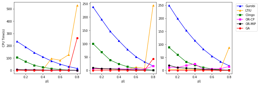
Refer to caption — Figure 1: CPU Time(s) for solving Max Cardinality SMTI $p2=0.2$ , $0.5$ , and $0.8$ with $n=100$

Figure 1 provides a comparison of the different approaches with respect to the CPU time for $n=50$ . It can be observed that, for most instances, these approaches (except for Gurobi) are comparable to each other, and that the local search methods takes more time for larger values of $p1$ (when the preference lists are less incomplete). For $n=100$ , we can observe in Table 5 that, for smaller values of $p1<0.7$ , GA is more efficient, whereas, for larger values of $p1\geq 0.7$ , Google-OR Tools MIP and Clingo are more efficient.

Table 7: Sex Equal SMTI: Average CPU-Times (in seconds) for

n=50

Solver		$p2$

	$p1$	0.1	0.2	0.3	0.4	0.5	0.6	0.7	0.8	0.9
OR-MIP	0.1	0.72	1.04	1.25	1.76	2.74	3.63	4.72	5.01	2.73
	0.2	0.58	0.63	1.03	2.17	1.78	2.23	4.24	7.05	1.91
	0.3	0.5	0.67	0.82	1.63	2.2	2.23	4.22	2.84	1.46
	0.4	0.4	0.46	0.59	0.96	1.54	1.38	2.58	3.68	3.61
	0.5	0.33	0.36	0.45	0.64	0.96	1.56	2.05	1.72	1.76
	0.6	0.26	0.27	0.37	0.7	0.76	0.74	1.27	0.87	0.85
	0.7	0.2	0.21	0.29	0.38	0.43	0.64	0.51	0.58	0.6
	0.8	0.16	0.17	0.17	0.2	0.26	0.31	0.26	0.3	0.48
OR-CP	0.1	5.42	4.43	5.68	3.94	7.45	7.56	9.35	17.75	98.13
	0.2	4.09	3.28	4.5	6.35	4.95	6.77	6.61	52.67	135.68[8]
	0.3	3.17	3.47	4.8	3.6	4.61	6.52	8.7	23.33	92.72[3]
	0.4	2.62	3.09	3.61	2.6	5.21	5.95	6.46	18.97	191.51[6]
	0.5	1.94	2.49	2.84	2.79	3.2	3.77	9.24	33.07	370.18[4]
	0.6	1.69	1.69	2.38	1.85	3.2	7.63	28.06	192.73	TO
	0.7	1.3	1.65	1.58	2.22	1.94	2.28	64.26	738.98[4]	487.86[5]
	0.8	0.86	1.21	1.03	1.05	1.67	15.24	6.69	83.98	578.02[7]
Clingo	0.1	TO	TO	TO	TO	TO	TO	TO	TO	TO
	0.2	TO	TO	TO	TO	TO	TO	TO	TO	TO
	0.3	TO	TO	TO	TO	TO	TO	TO	TO	TO
	0.4	1909.7[1]	TO	877.16[2]	TO	TO	TO	TO	TO	TO
	0.5	1305.27[2]	592.94[3]	297.8[2]	1658.6[1]	953.01[1]	TO	1182.33[2]	1437.34[3]	TO
	0.6	835.24[7]	656.42	1159.53[4]	910.1[4]	1093.83[4]	1048.79[8]	722.22[7]	758.89[3]	TO
	0.7	82.61	70.12	240.72	211.46	115.87	245.94	906.8[8]	488.83[4]	896.77[2]
	0.8	6.98	9.33	19.6	13.45	17.54	70.72	34.5	211.64	356.36[7]

TO: Timeout (over 2000 seconds)

Table 8: Egalitarian SMTI: Average CPU-Times (in seconds) for

n=50

		$p2$

Solver	$p1$	0.1	0.2	0.3	0.4	0.5	0.6	0.7	0.8	0.9
OR-MIP	0.1	0.64	0.7	0.73	0.78	0.81	0.86	1.05	1.29	1.8
	0.2	0.51	0.54	0.58	0.61	0.7	0.78	0.77	2.07	1.63
	0.3	0.42	0.46	0.47	0.52	0.59	0.61	0.85	2.04	6.26
	0.4	0.33	0.35	0.37	0.41	0.57	0.66	1.95	2.3	2.57
	0.5	0.27	0.27	0.29	0.38	0.33	0.45	0.65	2.62	4.38
	0.6	0.21	0.21	0.23	0.28	0.28	0.48	0.48	0.95	1.61
	0.7	0.16	0.16	0.17	0.19	0.21	0.21	0.4	0.96	1.42
	0.8	0.12	0.13	0.13	0.13	0.14	0.15	0.16	0.23	0.31
OR-CP	0.1	3.57	4.72	5.14	5.09	9.1	38.99[9]	488.9[6]	TO	TO
	0.2	4.11	4.17	4.66	4.54	6.92	231.5[9]	693.63[6]	TO	TO
	0.3	3.48	3.28	3.28	4.13	9.58	160.73[9]	211.32[4]	TO	TO
	0.4	2.52	2.4	2.94	3.55	25.58	204.4	924.95[4]	TO	TO
	0.5	1.78	2.06	2.28	3.07	6.02	132.39	292.09[4]	TO	TO
	0.6	1.41	1.76	2.34	2.89	6.55	309.16	1141.35[5]	TO	TO
	0.7	1.13	1.52	1.62	3.54	3.33	50.84	730.15[3]	TO	1913.49[1]
	0.8	1.01	1.32	1.0	1.37	2.68	46.22[8]	598.16[8]	613.27[3]	362.67[1]
Clingo	0.1	5.75	5.67	5.78	5.88	5.95	6.13	6.01	5.55	4.02
	0.2	3.82	3.86	3.88	3.96	4.05	4.13	3.94	3.6	2.5
	0.3	2.4	2.34	2.38	2.47	2.38	2.54	2.38	2.16	1.56
	0.4	1.4	1.41	2.37	1.41	1.44	1.45	1.48	1.41	1.49
	0.5	0.81	0.76	0.77	0.79	0.78	0.83	0.72	0.66	0.42
	0.6	0.41	0.37	0.4	0.39	0.36	0.38	0.36	0.315	0.2
	0.7	0.17	0.17	0.16	0.16	0.16	0.17	0.14	0.13	0.1
	0.8	0.06	0.07	0.07	0.06	0.06	0.06	0.06	0.06	0.04

TO: Timeout (over 2000 seconds)

For Sex-Equal and Egalitarian SMTI, we have compared the ILP approach using Google-OR Tools MIP, the CP approach using Google-OR Tools CP, and the ASP approach using Clingo. The results are shown in Tables 7 and 8 for $n=50$ .

For Sex-Equal SMTI, we observe that the average CPU times are larger for the CP and ASP approaches when compared with the Max Cardinality SMTI experimental results (Table 3). Also, note that there is a larger number of instances that could not be solved with these approaches within the given time threshold. In the table, the numbers in square brackets denote how many of the 10 instances could be solved. The ILP approach, on the other hand, performs better for Sex-Equal SMTI.

For Egalitarian SMTI, we observe that the average CPU times are larger for the CP approach when compared with the Max Cardinality SMTI experimental results (Table 3). Also, note that there is a larger number of instances that could not be solved with this approach within the given time threshold. The ASP and ILP approaches, on the other hand, perform better for Egalitarian SMTI.

It is interesting to observe that Clingo has better results for Egalitarian SMTI and Max Cardinality SMTI, compared to Sex-Equal SMTI. This may be related to the objective functions: Sex-Equal SMTI aims to minimize the sum of absolute values of differences of nonnegative numbers, whereas Egalitarian SMTI and Max Cardinality SMTI aim to minimize the sum of nonnegative numbers. The large CPU times for the ASP approach for Sex-Equal SMTI could also be due to the use of aggregates in weak constraints.

7 Conclusion

We have conducted an empirical study to compare different approaches to solve hard instances of SMTI: Max Cardinality SMTI, Sex-Equal SMTI, and Egalitarian SMTI. For that, we have introduced formulations of these problems in Answer Set Programming utilizing weak constraints, and implemented them for Clingo. We have adapted an existing Integer Linear Programming model of Max Cardinality SMTI, for other optimization variants of SMTI, and implemented them for Gurobi and Google-OR Tools (MIP and CP). We have also implemented two different existing local search algorithms to solve Max Cardinality SMTI, with slight adaptations. We have compared these approaches empirically over randomly generated instances.

We have also performed experiments to compare Answer Set Programming with Propositional Satisfiability, over SMTI instances. For the latter, we have utilized Cmodels with the SAT solver ZChaff, and SAT-E implementation with the SAT solver Lingeling.

There are several important discussions. First of all, modeling is an important step in all these problem-solving methods. For that reason, we have utilized the existing and empirically evaluated models in the literature, for SAT, ILP and local search. We have come up with our own ASP formulation for SMTI variants after trying different formulations and considering elaboration tolerance, as the existing ASP formulations of the stable marriage problems used as benchmarks in the ASP competitions address SMT problem (a tractable variant of SM Irving 1994).

Although Google-OR Tools provide a CP solver that takes as input (almost the same) ILP formulations of SMTI problems, we think it will be interesting to introduce CP formulations of these problems (e.g., in the spirit of Gent and Prosser 2002) and experiment with some other CP solvers. Similarly, although Cmodels provides a SAT-based method to solve SMTI instances, it is hinted by our experiments with the SAT encodings of SMTI by Drummond et al. 2015 that it will be worthwhile to compare our results with different SAT encodings of SMTI (e.g., in the spirit of Gent et al. 2002) and to extend SAT-E to solve optimization variants. These studies are part of our future work.

Regarding the experimental results for optimization variants, it is interesting to observe that the declarative methods (ASP, ILP, CP) are more promising compared to the local search algorithms as the problems get harder with more ties and incompleteness. It is also interesting to observe that the ASP approach using Clingo, and the ILP approach using Google-OR Tools MIP are significantly different from each other for Egalitarian SMTI and Sex-Equal SMTI: some problems cannot be solved by one approach in 2000 seconds, while they can be solved by the other approach in a few seconds. This may suggest a portfolio of ASP, CP, ILP solutions for hard SMTI problems.

We believe that comparing different (but closely related) methods to solve hard problems is valuable to better understand their strengths Cayli et al. 2008; Coban et al. 2008; Dovier et al. 2009; Erdem et al. 2020. Our study of the hard variants of SMTI problems contributes to this line of research, not only by providing models and implementations but also by providing benchmarks for future studies.

Acknowledgments.

We would like to thank Ian Gent, David Manlove, Andrew Perrault and Patrick Prosser for useful discussions and sharing their software with us. We would also like to thank anonymous reviewers for their valuable comments.

Appendix A Algorithms

Algorithm 1 LTIU

Input: An SMTI instance of size $n$ , step limit $S$
Output: A matching $\mu$

\mu\leftarrow\text{a randomly generated matching}

\mu_{best}\leftarrow\mu

step\leftarrow 0

while

step<S

\mu

is a perfect matching then

\mu_{best}\leftarrow\mu

break

bps\leftarrow\{(m,w)|(m,w)

is an undominated blocking pair

\}

bps

is empty then

\mu

is better than

\mu_{best}

then

\mu_{best}\leftarrow\mu

\mu\leftarrow\text{a randomly generated matching}

else

neighbors\leftarrow\{

removing

(m,w)

from

\mu|(m,w)\in bps\}

pick a random number

r

(0,1)

r<p

then

\mu\leftarrow

a random matching in

neighbors

else

eval_{\mu}\leftarrow

number of singles

+

number of blocking pairs in

\mu

for

n\in neighbors

eval_{n}\leftarrow

number of singles

+

number of blocking pairs in

n

eval_{\mu}>argmin(eval)

then

\mu\leftarrow

a random neighbor

n

such that

eval_{n}=argmin(eval)

else

\mu\leftarrow

a random matching in

neighbors

step=step+1

return

\mu_{best}

Algorithm 2 Adapted Genetic Algorithm

Input: An SMTI instance $I$ , probability for crossover $p$ , probability for mutation $m$ , number of evolution rounds $n$ and size of population $S$

Output: A matching $\mu$

population\leftarrow\emptyset

for

i\leftarrow 1

S

\mu_{0}=

obtain a matching by applying DA on

I

add

\mu_{0}

population

for

i\leftarrow 1

evolution\ rounds

temporary\ population\leftarrow population

select pairs of solutions based on crossover probability and perform cycle crossover operation

for

solution\in temporary\ population

select a random number

r

(0,1)

r<m

then

mutate

solution

population\leftarrow

best solutions from temporary population

return

\mu\leftarrow

best solution in population

Appendix B Further Experimental Results

Table 9: Average number of atoms for varying

p1

and

p2

values with

n=50

Solver		$p2$

	$p1$	0.1	0.2	0.3	0.4	0.5	0.6	0.7	0.8	0.9
Cmodels	0.1	113425	112634	112320	110987	111095	109762	108012	104989	96243
	0.2	89963	90285	90230	89101	88298	87244	85941	83127	7602
	0.3	71035	70487	70567	70404	69397	69143	67309	64401	57927
	0.4	53118	52825	51973	52700	51603	51357	49781	48818	43102
	0.5	38439	37674	37980	37733	37144	37668	34827	33615	30541
	0.6	26444	25382	26313	25192	24580	24654	23674	22664	19953
	0.7	15863	15638	15549	15338	15134	15239	14381	14004	12168
	0.8	8078	8315	8229	7929	8014	7647	7400	7004	6373
SAT-E	0.1	9022	8997	8984	8931	8926	8849	8758	8572	7963
	0.2	7969	7991	7988	7946	7901	7858	7783	7573	7086
	0.3	7013	6995	7006	6994	6941	6951	6823	6658	6156
	0.4	5986	5972	5931	5958	5911	5891	5791	5745	5234
	0.5	5001	4952	4982	4973	4933	4975	4787	4666	4317
	0.6	4049	3960	4052	3966	3914	3935	3856	3782	3425
	0.7	3004	2990	2979	2974	2962	2960	2899	2850	2635
	0.8	1975	2024	2013	1970	1991	1957	1920	1861	1716

Table 10: Average number of clauses for varying

p1

and

p2

values with

n=50

Solver		$p2$

	$p1$	0.1	0.2	0.3	0.4	0.5	0.6	0.7	0.8	0.9
Cmodels	0.1	1296263	1279570	1276494	1254057	1255637	1229722	1191007	1129910	962283
	0.2	937668	937568	935593	919152	905123	887740	864279	813669	681242
	0.3	670565	659872	660876	659103	641055	637263	609766	562206	464503
	0.4	443675	439157	428319	435531	421185	417162	395655	377376	297961
	0.5	280194	271381	274901	270723	263916	268156	237253	221306	181749
	0.6	164589	154443	162863	152339	147149	146310	137174	124952	98137
	0.7	79703	77568	77378	75205	73489	73914	67096	62831	48854
	0.8	31065	31959	31535	29783	29984	27705	26257	23537	19860
SAT-E	0.1	124392	123861	123903	122977	123803	123371	123251	123285	121668
	0.2	99573	100199	100467	99706	99439	99280	99371	98668	98449
	0.3	79429	79100	79484	79675	79133	79664	78818	78203	76368
	0.4	60204	60081	59432	60498	59797	60148	59490	60299	58423
	0.5	44271	43583	44159	44155	43889	44973	42697	42663	42386
	0.6	31061	29994	31231	30205	29783	30322	29808	29820	28736
	0.7	19138	18983	18981	18931	18908	19254	18798	19014	17933
	0.8	10040	10403	10369	10090	10306	10086	9972	9849	9523

References

Alkan and Gale (2003) Alkan, A. and Gale, D. 2003. Stable schedule matching under revealed preference. Journal of Economic Theory 112, 2, 289–306.
Alkan and Moulin (2003) Alkan, A. and Moulin, H. 2003. Mathematical theories of allocation of discrete resources: equilibria, matchings, mechanisms. Elsevier.
Biere (2010) Biere, A. 2010. Lingeling, Plingeling, PicoSAT and PrecoSAT at SAT race 2010. Tech. rep., FMV Technical Reports 10/1.
Biere et al. (2009) Biere, A., Heule, M., van Maaren, H., and Walsh, T., Eds. 2009. Handbook of Satisfiability. Frontiers in Artificial Intelligence and Applications, vol. 185. IOS Press.
Brewka et al. (2016) Brewka, G., Eiter, T., and Truszczynski, M. 2016. Answer set programming: An introduction to the special issue. AI Magazine 37, 3, 5–6.
Cayli et al. (2008) Cayli, M., Karatop, A. G., Kavlak, A. E., Kaynar, H., Ture, F., and Erdem, E. 2008. Solving challenging grid puzzles with answer set programming. In Proc. of the Int’l Workshop on Answer Set Programming (ASP’07).
Coban et al. (2008) Coban, E., Erdem, E., and Ture, F. 2008. Comparing ASP, CP, ILP on two challenging applications: wire routing and haplotype inference. In Proc. of the Int’l Workshop on Logic and Search (LaSh’08).
Delorme et al. (2019) Delorme, M., García, S., Gondzio, J., Kalcsics, J., Manlove, D. F., and Pettersson, W. 2019. Mathematical models for stable matching problems with ties and incomplete lists. Eur. J. Oper. Res. 277, 2, 426–441.
Dovier et al. (2009) Dovier, A., Formisano, A., and Pontelli, E. 2009. An empirical study of constraint logic programming and answer set programming solutions of combinatorial problems. J. Exp. Theor. Artif. Intell. 21, 2, 79–121.
Drummond et al. (2015) Drummond, J., Perrault, A., and Bacchus, F. 2015. SAT is an effective and complete method for solving stable matching problems with couples. In Proc. of IJCAI. 518–525.
Erdem et al. (2020) Erdem, E., Fidan, M., Manlove, D. F., and Prosser, P. 2020. A general framework for stable roommates problems using answer set programming. Theory Pract. Log. Program. 20, 6, 911–925.
Erdem and Lifschitz (2003) Erdem, E. and Lifschitz, V. 2003. Tight logic programs. Theory Pract. Log. Program. 3, 4-5, 499–518.
Erdil and Ergin (2008) Erdil, A. and Ergin, H. 2008. What’s the matter with tie-breaking? improving efficiency in school choice. American Economic Review 98, 3, 669–89.
Gale and Shapley (1962) Gale, D. and Shapley, L. S. 1962. College admissions and the stability of marriage. The American Mathematical Monthly 69, 1, 9–15.
Gebser et al. (2019) Gebser, M., Kaminski, R., Kaufmann, B., and Schaub, T. 2019. Multi-shot ASP solving with clingo. Theory Pract. Log. Program. 19, 1, 27–82.
Gelain et al. (2013) Gelain, M., Pini, M. S., Rossi, F., Venable, K. B., and Walsh, T. 2013. Local search approaches in stable matching problems. Algorithms 6, 4, 591–617.
Gent and Prosser (2002) Gent, I. P. and Prosser, P. 2002. An empirical study of the stable marriage problem with ties and incomplete lists. In Proc. of ECAI. 141–145.
Gent et al. (2002) Gent, I. P., Prosser, P., Smith, B., and Walsh, T. 2002. SAT encodings of the stable marriage problem with ties and incomplete lists. In Proc. of SAT. 133–140.
Giunchiglia et al. (2004) Giunchiglia, E., Lierler, Y., and Maratea, M. 2004. SAT-based answer set programming. In Proc. of AAAI. 61–66.
Gomes et al. (2007) Gomes, C. P., Kautz, H., Sabharwal, A., and Selman, B. 2007. Chapter 2: Satisfiability solvers. Handbook of Knowledge Representation. 89–134.
Haas (2020) Haas, C. 2020. Two-sided matching with indifferences: Using heuristics to improve properties of stable matchings. Computational Economics.
Holland (1992) Holland, J. H. 1992. Adaptation in Natural and Artificial Systems: An Introductory Analysis with Applications to Biology, Control and Artificial Intelligence. MIT Press.
Irving (1994) Irving, R. W. 1994. Stable marriage and indifference. Discrete Applied Mathematics 48, 3, 261–272.
Iwama et al. (1999) Iwama, K., Miyazaki, S., Morita, Y., and Manlove, D. 1999. Stable marriage with incomplete lists and ties. In Automata, Languages and Programming, J. Wiedermann, P. van Emde Boas, and M. Nielsen, Eds. Springer Berlin Heidelberg.
Jaffar and Lassez (1987) Jaffar, J. and Lassez, J.-L. 1987. Constraint logic programming. In Proc. of POPL. 111––119.
Järvisalo et al. (2012) Järvisalo, M., Berre, D. L., Roussel, O., and Simon, L. 2012. The international SAT solver competitions. AI Mag. 33, 1, 89–92.
Kantorovich (1960) Kantorovich, L. V. 1960. Mathematical methods of organizing and planning production. Management Science 6, 4, 366–422.
Kato (1993) Kato, A. 1993. Complexity of the sex-equal stable marriage problem. Japan Journal of Industrial and Applied Mathematics 10, 1, 1–19.
Lifschitz (2002) Lifschitz, V. 2002. Answer set programming and plan generation. Artificial Intelligence 138, 1-2, 39–54.
Lin and Zhao (2004) Lin, F. and Zhao, Y. 2004. ASSAT: computing answer sets of a logic program by SAT solvers. Artif. Intell. 157, 1-2, 115–137.
Lin and Kernighan (1973) Lin, S. and Kernighan, B. W. 1973. An effective heuristic algorithm for the traveling-salesman problem. Oper. Res. 21, 2, 498––516.
Manlove et al. (2002) Manlove, D. F., Irving, R. W., Iwama, K., Miyazaki, S., and Morita, Y. 2002. Hard variants of stable marriage. Theoretical Computer Science 276, 1-2, 261–279.
Manlove and O’malley (2015) Manlove, D. F. and O’malley, G. 2015. Paired and altruistic kidney donation in the uk: Algorithms and experimentation. ACM J. Exp. Algorithmics 19.
Marek and Truszczyński (1999) Marek, V. W. and Truszczyński, M. 1999. Stable models and an alternative logic programming paradigm. In The Logic Programming Paradigm. Springer, 375–398.
Moskewicz et al. (2001) Moskewicz, M., Madigan, C., Zhao, Y., Zhang, L., and Malik, S. 2001. Chaff: engineering an efficient sat solver. In Proc. of IEEE DAC. 530–535.
Niemelae (1999) Niemelae, I. 1999. Logic programs with stable model semantics as a constraint programming paradigm. Annals of Mathematics and Artificial Intelligence 25, 3, 241–273.
Rossi et al. (2006) Rossi, F., Beek, P. v., and Walsh, T. 2006. Handbook of Constraint Programming (Foundations of Artificial Intelligence). Elsevier Science Inc.
Roth et al. (2005) Roth, A. E., Sonmez, T., and Utku Unver, M. 2005. Pairwise kidney exchange. Journal of Economic Theory 125, 2, 151–188.
Roth and Sotomayor (1992) Roth, A. E. and Sotomayor, M. 1992. Chapter 16: Two-sided matching. Handbook of Game Theory with Economic Applications, vol. 1. Elsevier, 485–541.
Selman and Gomes (2006) Selman, B. and Gomes, C. P. 2006. Hill-climbing Search. American Cancer Society.
Simons et al. (2002) Simons, P., Niemelae, I., and Soininen, T. 2002. Extending and implementing the stable model semantics. Artif. Intell. 138, 1, 181–234.
Van Hentenryck (1989) Van Hentenryck, P. 1989. Constraint Satisfaction in Logic Programming. MIT Press, Cambridge, MA, USA.