Deep Pairwise Learning To Rank For Search AutocompleteDOI: 10.1145/1122445.1122456CCS: Information systems Information retrieval Retrieval models and ranking Learning to rank
Abstract.
Autocomplete (a.k.a “Query Auto-Completion”, “AC”) suggests full queries based on a prefix typed by customer. Autocomplete has been a core feature of commercial search engine. In this paper, we propose a novel context-aware neural-network based pairwise ranker (DeepPLTR) to improve AC ranking, DeepPLTR leverages contextual and behavioral features to rank queries by minimizing a pairwise loss, based on a fully-connected neural network structure. Compared to LambdaMART ranker, DeepPLTR shows +3.90% MeanReciprocalRank (MRR) lift in offline evaluation, and yielded +0.06% (p < 0.1) Gross Merchandise Value (GMV) lift in an Amazon’s online A/B experiment.
Keywords:
pairwise learning To rank, neural networks, query embedding1. Introduction
Autocomplete is a common feature of most modern commercial search engines. It refers to the task of suggesting full queries after customer typed a prefix of a few characters (Cai et al. 2016). Study shows that AC feature can significantly reduce the number of characters typed (Zhang et al. 2015). An Autocomplete system generally consists of 2 steps: Matching and Ranking. Matching refers to generating query candidates given a typed prefix. Ranking refers to ranking the candidates. In this paper, we focus on the Ranking step and propose a NN-based online deep pairwise learning to rank (DeepPLTR) ranker. Our work makes the following contributions:
- •
Propose a novel NN-based ranker to rank queries by minimizing pairwise loss.
- •
Propose a novel method to incorporate the contextual signals into ranking.
The paper is organized as follows: Section 2 describes the related work in the literature; Section 3 proposes the DeepPLTR model; Section 4 presents the datasets, evaluation methods and experiments; Section 5 summarizes our work and discusses possible future research directions.
2. Related Work
A detailed survey of AC work could be found in (Cai et al. 2016), which categories the Autocomplete into 2 types: heuristic approaches and learning-based approaches. Heuristic approaches use fixed algorithms to compute a ranking score for each query. Learning-based approaches treat the Autocomplete as a ranking problem, and rely on the research of learning-to-rank(LTR) field (Liu et al. 2009), it requires a large number of training samples and features, and generally outperforms the heuristic approaches (Cai et al. 2016). Ranking features can be categorized into 3 types: time-senstive features, personalized features and contextual features. Time-sensitive features are based on query popularity and could change over time. Personalized features, such as location, are typically limited and hard to access. Contextual features rely on the customer’s previous activity and are easy to extract from the search logs. Incorporating contextual signal into model is challenging. Bar-Yossef and Kraus (Bar-Yossef and Kraus 2011) use user’s previous queries in their context-aware AC. Shokouhi (Shokouhi 2013) used a combination of context-based textual features and personalized features in their context-aware AC, and showed that the user’s long term search history and location are most effective signals. NN-based approach is also widely studied for AC ranking task. Session-based, personalized, and attention-based models were proposed in (Jiang et al. 2018) Fiorini and Lu (Fiorini and Lu 2018) extracted user history based features and time features as an input to an RNN model. Latest approach for AC ranking was proposed by Manojkumar et al. (Kannadasan and Aslanyan 2019), this approach was to train query and context embeddings on the reformulations behavior in search sessions, calculate contextual similarity features from the context and query embeddings, and then feed contextual features to a LambdaMART (Burges 2010) ranker. This embedding approach is similar to the “whole query embedding” proposed in this paper when computing contextual similarity features.
3. Deep Pairwise Learning To Rank Model
In this section, we first describe a common labeling strategy for pairwise AC ranking task, then demonstrate the DeepPLTR architecture and ranking loss, then we propose a scalable approach to learn whole query embeddings and apply it to generate contextual features for ranking model.
3.1. Training Sample Generation

AC session dataset is the main source to extract training samples. One AC session consists of aggregated impression logs that starts from the first keystroke in search box, all the way until customer submits the query. AC session has been attributed with the right metrics (GMV, sales, clicks etc) to each impression, as the metrics are only observed after customer submits the query, e.g. viewing or purchasing products. We propose a similar labeling strategy: we start by sampling a set of ac sessions. For each ac session, we assume that the query that was eventually submitted is the only right (or the most relevant) query, which should have been suggested right after the first keystroke and all the way until submission. With this assumption in mind, we obtained all the impressed queries from each suggestion; for each pair of <prefix, completion list> constructed this way, we assign positive label to the query submitted by user at the end (if it appears in the list) as relevant keywords and negative label to other impressed queries as irrelevant keywords. Then we grouped these positive and negative keywords from the same impression into pairs. Figure 1 provides an example: here we sampled one series of impression logs in which the user had submitted “hangers” as query. For each prefix, the only query that is assigned a positive label is specified with a checkmark (✓), and the query that is assigned a negative label is specified with a crossmark (✗). The attribution of the pairs is set to 100 as GMV attribution is $100 for this AC session.

3.2. Model Architecture
Given the extracted pairs, the DeepPLTR architecture is designed as in Figure 2. It’s a typical RankNet (Burges 2010) structure based on fully-connected neural network (Sainath et al. 2015). Different from RankNet (Burges 2010), it adds a context representation layer, which is scalable to host contextual signals. Most of the dense layers are weight-sharing as they represents the same concepts (e.g. query representation, query-context representation). The LSTM (Gers et al. 1999) layer captures the sequential signal of the time series related features, which has better performance than dense structure. The final output layer applies the sigmoid activation (Han and Moraga 1995) function and binary cross-entropy loss (De Boer et al. 2005) by subtracting the two ranking scores from previous layers. After fine-tuning the parameters through a hyper-parameter tuning process, query representation layer has 128 neurons, LSTM has 16 neurons, context representation layer has 128 neurons, and dropout layer ratio is 0.1. All dense layers apply the ReLU (Nair and Hinton 2010) activation function. The output labels are set to 1, as the model is trained based on positive keywords ranking higher than negative keywords.
3.3. Ranking Loss
Ranking loss is composed of 3 parts: binary cross entropy loss, and sample weights. Binary cross entropy loss represents the loss when reversing the ranking order of positive-negative pair. Sample weights represent the optimization target, for example, if the model optimizes GMV, we set GMV as the weight of each pair. considers the change in NDCG when swapping the ranking positions of positive and negative keywords, so that a keyword pair more separated in the ranking list gets a larger loss. Then we define the loss as below:
denotes the full set of pairs from Section 3.1. denotes the positive keywords and denotes the negative keywords. denotes the sample weight of the pair. is the learned ranking function which minimizes the ranking loss. and denote the ranking score of the keywords and . denotes the change in NDCG when swapping the positions of keywords and . denotes the ranking position of the keywords (. denotes the output label. denotes the probability that the positive keyword is ranked above the negative keyword , which serves the purpose of a contrastive loss that helps distinguish the positive keyword from the negative keyword: when the difference between and is larger, will be larger. Then we have:
|
|
where is defined as
| (1) |
and is defined as:
| (2) |
Given is always 1 and , we simplify the loss from Eq. (3.3) as:
| (3) |
|
3.4. Query Representation And Contextual Features
We construct contextual features by calculating the cosine distance between candidate queries and past search queries using pre-trained query embeddings. In this paper, we use the publicly available library (Bojanowski et al. 2017) to learn the query embeddings. We use the skipGram model where the goal is to independently predict the presence or absence of the context words. The problem is framed as a binary classification task. For the word at position , considers all context words as positive examples and sample random negatives words from dictionary as described in (Bojanowski et al. 2017; Mikolov et al. 2013). It uses the negative log likelihood, as the binary logistic loss. The objective function is defined as:
| (4) |
where is the target word, is the context word, is context words, and is a set of negative examples sampled from the vocabulary. The scoring function is the scalar product between word and context vectors: , where vectors and corresponding to words and context words respectively.
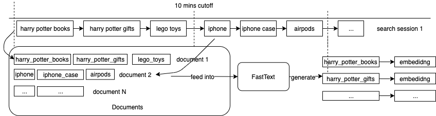
Our goal is to learn scalable embeddings across different marketplaces and languages. For US, we collect the past 60 days’ search sessions (a sequential search actions), and divide each session into multiple sequences of queries, such that no consecutive queries in a sequence are separated by > 10 minutes. We normalize queries by removing special characters and replace space character ‘ ’ to ‘_’. We treat each query as a “word”, and sequences of queries as a “document”, and feed them into (Bojanowski et al. 2017) to train and generate embeddings with 50 dimensions. We call it the whole query embedding approach. Figure 3 illustrates the whole query embedding generation process. Compared to the token embedding approach, whole query embedding is a scalable approach as it generates query embeddings WW without language specific processing, e.g. tokenization for Chinese and Japanese. Then at online, we apply the pre-trained embeddings to calculate the cosine similarity between each candidate and past search query as contextual features. In particular, given recently searched query and candidate , query embedding . .
4. Experiments
4.1. Dataset and Experiment Settings
To conduct experiments, we follow the labeling strategy described in Section 3.1 to extract 77M training pairs, and 11M validation pairs from AC sessions which lead to purchase events (GMV ) during a week of US data in 2020. This gives us a good coverage of user context features to learn deep model. In order to benchmark on MRR and NDCG, we collect 150k impression logs with ground truth as the test datasets in Feb. 8, 2020. Different models are trained and evaluated with the same sampled data.
4.2. Benchmark Rankers
To evaluate DeepPLTR, we constructed 4 benchmark rankers:
MPC Ranker: the MostPopularCompletion ranker (Bar-Yossef and Kraus 2011), which is a common benchmark for AC task. It ranks queries by the decayed search popularity of the query.
MPGC Ranker: the MostPopularGMVCompletion ranker, which ranks by the decayed GMV of query. It’s designed to benchmark with GMV-optimized model.
LambdaMART Ranker (context-aware): train a LambdaMART ranker using XGBoost library (Chen and Guestrin 2016) with the same features as DeepPLTR. From which, we will learn whether NN architecture could improve performance. We set pairwise loss as the optimization target, and fine-tuned number of trees as 150 and max depth as 6 to XGBoost to train the model. We treat this as a baseline ranker.
DeepPLTR-NDCG Ranker (context-aware): train a DeepPLTR excluding loss in the Eq. 3 to learn the position impact.
4.3. Evaluation Metrics
MeanReciprocalRank: the average of the reciprocal rank of the target queries in the AC results weighed on the business metrics. Given a test dataset , the MRR for ranker is computed as:
| (5) |
where represents the user context at time , represents the target query, and represents the sample weight. The function computes the rank of the relevant query based on the order created by algorithm . The relevant query refers to the clicked query in AC.
NormalizedDiscountedCumulativeGain: Discounted Cumulative Gain () represents the usefulness or gain of the query based on its position in the ranked list. Given AC task having one relevant query, will always be 1, so NDCG@p can be simplified as below:
| (6) |
where denotes the rank, is the relevance of query at rank , and is the sample weight.
4.4. Results
To learn the impact of contextual signals on the model’s performance, we construct three versions of test samples: All Samples (AS), Samples With Past Searches (SWPS) and Samples Without Past Searches (SWOPS). Evaluation metrics are set to MRR, NDCG@1, NDCG@3.
| Model | MRR | NDCG@1 | NDCG@3 |
|---|---|---|---|
| MPC | 0.469(-16.84%) | 0.293(-22.49%) | 0.464(-18.74%) |
| MPGC | 0.488(-13.48%) | 0.308(-18.52%) | 0.485(-15.06%) |
| LambdaMART | 0.564 | 0.378 | 0.571 |
| DeepPLTR-NDCG | 0.577(+2.30%) | 0.400(+5.82%) | 0.584(+2.28%) |
| DeepPLTR | 0.586(+3.90%) | 0.409(+8.20%) | 0.594(+4.03%) |
| Model | MRR | NDCG@1 | NDCG@3 |
|---|---|---|---|
| MPC | 0.481(-16.20%) | 0.297(-23.06%) | 0.474(-18.56%) |
| MPGC | 0.505(-12.02%) | 0.315(-18.39%) | 0.502(-13.75%) |
| LambdaMART | 0.574 | 0.386 | 0.582 |
| DeepPLTR-NDCG | 0.570(-0.70%) | 0.385(-0.26%) | 0.580(-0.34%) |
| DeepPLTR | 0.572(-0.35%) | 0.388(+0.52%) | 0.581(-0.17%) |
| Model | MRR | NDCG@1 | NDCG@3 |
|---|---|---|---|
| MPC | 0.459(-17.45%) | 0.289(-22.10%) | 0.455(-19.04%) |
| MPGC | 0.474(-14.75%) | 0.303(-18.33%) | 0.470(-16.37%) |
| LambdaMART | 0.556 | 0.371 | 0.562 |
| DeepPLTR-NDCG | 0.582(+4.68%) | 0.413(+11.32%) | 0.587(+4.45%) |
| DeepPLTR | 0.598(+7.55%) | 0.427(+15.09%) | 0.606(+7.83%) |
Evaluation on AS are shown in Table 1. LambdaMART ranker outperforms the naive rankers (MPC, MPGC), which is expected with more advanced signals. DeepPLTR outperforms the LambdaMART by 3.90% in MRR, by 8.20% in NDCG@1, and by 5.99% in NDCG@3, showing that NN-based architecture imrpoves the performance. DeepPLTR outperforms DeepPLTR-NDCG, shows that considering position factor in ranking boosts the ranking performance.
Evaluation on SWOPS are shown in Table 2. LambdaMART ranker slightly outperforms DeepPLTR on , which shows that DeepPLTR has similar performance to LambdaMART ranker without past search history. LambdaMART ranker slightly outperforms PLTR, showing that device type feature improves performance. Evaluation on SWPS are shown in Table 3. DeepPLTR outperforms baseline by 7.55% in MRR and 15.09% in NDCG@1, showing that DeepPLTR can learn implicit ranking features based on past searches features. DeepPLTR boosts performance the most on SWPS samples.
We also conduct an online A/B experiment to compare the DeepPLTR and LambdaMART ranker, experiment shows DeepPLTR yields a +0.06% (p < 0.1) GMV lift compared to LambdaMART ranker, which demonstrates the DeepPLTR outperforms LambdaMART.
5. Conclusions and Future Work
In this paper, we have proposed a neural-network based pairwise ranker and ranking loss, and described a scalable approach to learn query embeddings using search session data. The architecture of DeepPLTR is scalable for accommodating a variety of ranking signals and can be applied to other search tasks such as product search. We conduct offline and online experiments to verify that DeepPLTR outperforms LambdaMART ranker. In the future, we will improve AC in several directions: 1) Incooporate richer contextual information, e.g. past product clicks & purchases; 2) Add exploration mechanism to explore unshown suggestions.
Acknowledgements.
We would like to thank the team members in Amazon Search: Trishul Chilimbi, Adam Kiezun, Wenyang Liu, Hsiang-Fu Yu, Erte Pan, Yun Hyokun, Zia Hasan, Pratik Lahiri, RJ, Yukun Lin, Haining Yu, Ben Wing, Hye Jin Jang for their support.References
- (1)
- Bar-Yossef and Kraus (2011) Ziv Bar-Yossef and Naama Kraus. 2011. Context-sensitive query auto-completion. In Proceedings of the 20th international conference on World wide web. 107–116.
- Bojanowski et al. (2017) Piotr Bojanowski, Edouard Grave, Armand Joulin, and Tomas Mikolov. 2017. Enriching word vectors with subword information. Transactions of the Association for Computational Linguistics 5 (2017), 135–146.
- Burges (2010) Christopher JC Burges. 2010. From ranknet to lambdarank to lambdamart: An overview. Learning 11, 23-581 (2010), 81.
- Cai et al. (2016) Fei Cai, Maarten De Rijke, et al. 2016. A survey of query auto completion in information retrieval. Foundations and Trends® in Information Retrieval 10, 4 (2016), 273–363.
- Chen and Guestrin (2016) Tianqi Chen and Carlos Guestrin. 2016. Xgboost: A scalable tree boosting system. In Proceedings of the 22nd acm sigkdd international conference on knowledge discovery and data mining. 785–794.
- De Boer et al. (2005) Pieter-Tjerk De Boer, Dirk P Kroese, Shie Mannor, and Reuven Y Rubinstein. 2005. A tutorial on the cross-entropy method. Annals of operations research 134, 1 (2005), 19–67.
- Fiorini and Lu (2018) Nicolas Fiorini and Zhiyong Lu. 2018. Personalized neural language models for real-world query auto completion. arXiv preprint arXiv:1804.06439 (2018).
- Gers et al. (1999) Felix A Gers, Jürgen Schmidhuber, and Fred Cummins. 1999. Learning to forget: Continual prediction with LSTM. (1999).
- Han and Moraga (1995) Jun Han and Claudio Moraga. 1995. The influence of the sigmoid function parameters on the speed of backpropagation learning. In International Workshop on Artificial Neural Networks. Springer, 195–201.
- Jiang et al. (2018) Danyang Jiang, Wanyu Chen, Fei Cai, and Honghui Chen. 2018. Neural Attentive Personalization Model for Query Auto-Completion. In 2018 IEEE 3rd Advanced Information Technology, Electronic and Automation Control Conference (IAEAC). IEEE, 725–730.
- Kannadasan and Aslanyan (2019) Manojkumar Rangasamy Kannadasan and Grigor Aslanyan. 2019. Personalized Query Auto-Completion Through a Lightweight Representation of the User Context. arXiv preprint arXiv:1905.01386 (2019).
- Liu et al. (2009) Tie-Yan Liu et al. 2009. Learning to rank for information retrieval. Foundations and Trends® in Information Retrieval 3, 3 (2009), 225–331.
- Mikolov et al. (2013) Tomas Mikolov, Ilya Sutskever, Kai Chen, Greg S Corrado, and Jeff Dean. 2013. Distributed representations of words and phrases and their compositionality. In Advances in neural information processing systems. 3111–3119.
- Nair and Hinton (2010) Vinod Nair and Geoffrey E Hinton. 2010. Rectified linear units improve restricted boltzmann machines. In Proceedings of the 27th international conference on machine learning (ICML-10). 807–814.
- Sainath et al. (2015) Tara N Sainath, Oriol Vinyals, Andrew Senior, and Haşim Sak. 2015. Convolutional, long short-term memory, fully connected deep neural networks. In 2015 IEEE International Conference on Acoustics, Speech and Signal Processing (ICASSP). IEEE, 4580–4584.
- Shokouhi (2013) Milad Shokouhi. 2013. Learning to personalize query auto-completion. In Proceedings of the 36th international ACM SIGIR conference on Research and development in information retrieval. 103–112.
- Zhang et al. (2015) Aston Zhang, Amit Goyal, Weize Kong, Hongbo Deng, Anlei Dong, Yi Chang, Carl A Gunter, and Jiawei Han. 2015. adaqac: Adaptive query auto-completion via implicit negative feedback. In Proceedings of the 38th international ACM SIGIR conference on research and development in information retrieval. 143–152.