Imaging from STIX visibility amplitudes
Abstract
Aims. To provide the first demonstration of STIX Fourier-transform X-ray imaging using semi-calibrated (amplitude-only) visibility data acquired during the Solar Orbiter’s cruise phase.
Methods. We use a parametric imaging approach by which STIX visibility amplitudes are fitted by means of two non-linear optimization methods: a fast meta-heuristic technique inspired by social behavior, and a Bayesian Monte Carlo sampling method, which, although slower, provides better quantification of uncertainties.
Results. When applied to a set of solar flare visibility amplitudes recorded by STIX on November 18, 2020 the two parametric methods provide very coherent results. The analysis also demonstrates the ability of STIX to reconstruct high time resolution information and, from a spectral viewpoint, shows the reliability of a double-source scenario consistent with a thermal versus nonthermal interpretation.
Conclusions. In this preliminary analysis of STIX imaging based only on visibility amplitudes, we formulate the imaging problem as a non-linear parametric issue we addressed by means of two high-performance optimization techniques that both showed the ability to sample the parametric space in an effective fashion, thus avoiding local minima.
Key Words.
Solar X-ray flares – X-ray telescopes – Astronomical techniques – Astronomy data reduction – Visibility functionAugust 11, 2026
1 Introduction
The solar corona is permanently heated to temperatures of several million degrees, well above the moderately hot solar surface which is around 6000 K. While the source of the energy that heats the corona has been early on identified as the solar magnetic field, the detailed process(es) of how the energy release is triggered and how energy is eventually dissipated into heat has been an ongoing research topic for many decades. The recently launched missions Parker Solar Probe and Solar Orbiter open new windows to unravel this mystery. Hard X-ray observations provide strong diagnostics of the hottest solar plasma and nonthermal electrons through the bremsstrahlung process, and therefore they play a key role in investigating the impulsive magnetic energy release in the corona during solar flares. While hard X-ray focusing optics has made great progress in the past years (Krucker et al. 2013, e.g.,), indirect imaging systems in hard X-rays have had great success with instruments such as the Hard X-ray Telescope on-board Yohkoh (Kosugi et al. 1992) and the Reuven Ramaty High Energy Solar Spectroscopic Imager (RHESSI) (Lin et al. 2002).
The Spectrometer/Telescope for Imaging X-rays (STIX) (Krucker et al. 2020) is a hard X-ray imaging-spectrometer onboard the Solar Orbiter spacecraft. STIX imaging uses an indirect Fourier technique in which the native form of the data is a set of angular Fourier components. Imaging-spectroscopy is based on the choice of the energy of the photons used as the input to the imaging process. The hardware includes a set of independent subcollimators, each consisting of a coarsely-pixelated photon detector with good energy resolution located behind a pair of widely separated grids whose joint transmission creates a large-scale Moiré pattern. Each Moiré pattern can be interpreted to measure a Fourier component of the incoming flux, termed a visibility, whose amplitude corresponds to the difference between the maximum and the minimum of the Moiré pattern and whose phase corresponds to the location of the peak of the Moiré pattern (Giordano et al. 2015; Massa et al. 2019). The angular frequency, which corresponds to each such visibility, is fixed by the choice of orientation and pitch of the corresponding grids. The choices can be divided into 10 groups, each of which corresponds to one of 10 logarithmically-spaced angular resolutions in the range 7.1 to 180 arcseconds as measured at 3 different orientations.
For a fully-calibrated instrument, the image reconstruction problem for STIX is therefore the linear Fourier inversion problem from limited data that can be addressed by means of regularization methods like interpolation/extrapolation (Perracchione et al. 2020), maximum entropy (Massa et al. 2020), or compressed sensing (Duval-Poo et al. 2018).
However, while the current calibration of the STIX imaging system is reliable for visibility amplitudes, the more complex phase calibration is just not yet available (while we are writing this paper, the calibration and validation process for STIX visibilities is in progress and will be finalized well in advance with respect to the beginning of the nominal phase of the mission in September 2021). Therefore, the current image reconstruction problem is the one of determining (partial) information on the flaring source from measurements of the visibility amplitudes only. Such a reconstruction problem has two main difficulties: 1) it is non–linear, and 2) no information on the source location can be retrieved from the amplitude of the Fourier transform alone. We point out that this situation is analogous to amplitude-only imaging in the early days of very long baseline radio interferometry (Pearson & Readhead 1984) as well as in other fields.
This study describes an approach to the solution of the STIX image reconstruction problem from visibility amplitudes, in which the flaring source is modelled by means of a limited number of simple but flare–appropriate parametric shapes (Dennis & Pernak 2009). We address the problem of source parameter estimation with two alternative methods. The first one is based on a stochastic optimization technique (Eberhart & Kennedy 1995) for solving the forward–fitting problem. It also relies on a confidence strip approach (Piana 1994) for computing parameter uncertainties, which has the advantage of being fast, but comes at the price of having to perturb multiple times the input data, often resulting in misinterpretations. The second one is a Bayesian technique (Sciacchitano et al. 2019), which produces full probabilistic description of the source parameters in a mathematically sound way, and often produces smaller uncertainties, but has higher computational cost. We point out that forward-fitting techniques have been already used within the framework of Fourier imagers missions. For example, a forward-fitting algorithm based on deterministic optimization is in the Solar Software (SSW) tree of the RHESSI mission (Aschwanden et al. 2003) and the Bayesian technique illustrated in Sciacchitano et al. 2018 has been validated against fully-calibrated RHESSI visibilities.
We illustrate the two parametric methods using STIX visibility amplitudes associated to a flaring event of the Sun in November 2020. The images provided by this example should not be considered as science products. However, this analysis may represent a timely demonstration of STIX imaging capabilities in terms of temporal and spectral resolution.
The plan of the paper is as follows. Section 2 introduces the visibility amplitude imaging problem. Section 3 describes the computational approach to its solution and Section 4 contains the results of the application of such approach to a set of experimental STIX observations. Our conclusions are offered in Section 5.
2 The visibility amplitude imaging problem
When a stable and calibrated imaging pipeline will become available, the STIX imaging problem will be described by
| (1) |
where is the incoming photon flux emitted from location on the solar disk, is the set of visibilities measured by the telescope in correspondence of the points on the -plane made of all angular frequencies, and is the imaging operator that maps the functions representing the flaring source into samples of their Fourier transform, i.e.
| (2) |
The STIX subcollimators will provide visibilities. We note that the STIX imaging problem, i.e. the one of reconstructing the photon flux from visibilities, is linear, but does not have a unique solution.
Unfortunately, the currently available calibration of the imaging system is limited to the visibility amplitudes, the phase calibration being more complex and therefore still under construction. The formal consequence of this limitation is that the STIX imaging operator at this stage is represented by
| (3) |
and therefore the imaging problem addressed in the present study is
| (4) |
where and should be intended as component-wise. This imaging problem is more challenging to solve than (1) for two key reasons: 1) it is non-linear, and 2) visibility amplitudes do not encode any information on the position of the flaring source. To overcome these limitations, we implemented forward–fitting procedures to estimate the parameters of three different parametric shapes of very simple architecture. Specifically, we have considered:
- •
A Gaussian circular source
(5) where is the total flux of the source, and is the Full Width at Half Maximum (FWHM). The set of parameters for this source is .
- •
A Gaussian elliptical source
(6) where is the total flux of the source, , , is the major FWHM and is the minor FWHM. Moreover,
(7) (8) where is the angle between the semi-major and the -axis measured counterclockwise. The set of parameters for the elliptical source is 11 1 We point out that we actually optimize the two auxiliary variables: and , satisfying and ..
- •
A double Gaussian circular source
(9) where is the total flux, , is the FWHM () and are the coordinates of the center of one source (the other is symmetric with respect to the origin). The set of parameters for the double circular source is .
The shapes of the three parametric sources are illustrated in Figure 1. In the next section we present the two computational methods for estimating the set of source parameters; without loss of generality, we will denote such set as , which is intended to be either , or , according to the estimated shape.
3 The approach to image reconstruction
The multivariate optimization problem in hard X-ray solar imaging is typically represented by the minimum problem
| (10) |
where is the so-called feasibility region for the imaging parameter and measures the square of the discrepancy between the experimental visibility amplitudes and the ones predicted by computing the Fourier transform of the source shape parameterized by . The solution of this problem usually relies on the RHESSI legacy (Lin et al. 2002) and, specifically, on the visfwdfit routine that computes the imaging parameters by means of a simplex approach. However, the number of visibilities provided by STIX is significantly smaller than the one provided by RHESSI and, at this stage of the calibration process, the information contained in STIX observations is even more limited. This is the reason why, in this first and preliminary study devoted to STIX imaging, we have implemented two more sophisticated approaches that have been explicitly designed in order to avoid local minima in the optimization process.
3.1 Particle Swarm Optimization
Particle Swarm Optimization (PSO) (Eberhart & Kennedy 1995; Qasem & Shamsuddin 2011) does not require any strong assumptions on the issue defined in (10), and takes advantage of being usually more robust than deterministic strategies (Nocedal & Wright 1999, see e.g.,) in presence of multiple local minima. To briefly review it, let us consider a group of particles or birds which are represented as points in the space . The goal of swarm intelligence is to model the trajectories of each single particle. Indeed, the target of a flock is to look for the maximum availability of food, i.e. the minimum of the objective function . The trajectory of each single bird is updated at each step of the algorithm by taking into account both its selfish and social behavior. Precisely, supposing that a particle visits some local minima then the other birds can either:
- i.
Move away from the flock towards the local minimum (selfish behavior), or
- ii.
Stay close to the flock (social behavior).
Assuming that the two behaviors are well-balanced, then the flock gradually changes its position until the global minimum is reached.
The IDL implementation was designed following the guidelines given by Mezura-Montes & Coello Coello 2011 and MATLAB R2019b. Specifically, given a first random initialization, at the -th iteration, each -th bird position is defined via its velocity and its best local position . Letting the global best position, the position of each particle is updated as
| (11) |
where
| (12) |
for , where , are randomly fixed and denotes the component-wise product. The parameters and are the acceleration coefficients and is the inertia weight that is adaptively updated in our implementation (Mezura-Montes & Coello Coello 2011).
Uncertainty quantification with PSO is determined by means of a confidence strip approach: several realizations of the input data are computed by randomly perturbing the experimental set of visibility amplitudes with Gaussian noise whose standard deviation is set equal to the errors on the measurements; for each realization PSO is applied; and, finally, the standard deviation of each optimized source parameter is computed.
3.2 Sequential Monte Carlo
The second approach to image reconstruction from STIX visibility amplitudes is based on a Bayesian source identification method (Sciacchitano et al. 2019) which has proven capable of assessing, on RHESSI data (Sciacchitano et al. 2018): 1) the likely number of sources in the image, 2) the parameters characterizing each source, and 3) the associated uncertainties.
Given the current restriction on the calibration of the imaging system, and the consequent loss of information on the position of the flaring source, we restrict here the usage of the Sequential Monte Carlo (SMC) method to the identification of one single shape per image, which is one of the three described in Section 2 (Fig. 1). The resulting method is an alternative approach to the one outlined in (10), as we are here interested in providing probabilistic estimates of the set of source-related parameters . In a Bayesian setting22 2 In a Bayesian setting, all the variables of the problem are considered as random variables, with information on their values encoded as their probability distributions. In the following we will use lower-case letters to indicate both the random variables and their specific values in a given instance., we need to describe the posterior distribution for the flare source parameters conditioned on the set of observed visibility amplitudes , which has the following form
| (13) |
Here, is the likelihood function, expressing the probability that the observed visibility amplitudes are produced by an image with parameters ; is the prior probability on the set of parameters; and is a normalisation factor.
The likelihood function is assumed to be (Hurford et al. 2002)
| (14) |
where the standard deviations are known. Statistical errors in the visibility data are directly inferred from photon statistics in the corresponding detectors. An additional allowance of is added in quadrature to account for systematic errors.
The choice for the prior distributions on the parameters is done according to Sciacchitano et al. 2018:
| (15) | |||
| (16) | |||
| (17) | |||
| (18) | |||
| (19) |
where indicates the field of view of the map.
As a consequence of these choices for prior and likelihood, the posterior probability density results to be an analytically intractable function on a high-dimensional space. Therefore, to compute it we use the SMC method (Sciacchitano et al. 2018), which produces a sample set that is approximately distributed according to the posterior, and can be used to make inference on the values of the various parameters. Once the algorithm converges, the parameters of the reconstructed map are computed by using the mean values of the posterior distributions (for the different parameters). The notable advantage of this algorithm is that it is able to realize uncertainty quantification in a very elegant way. In fact, the availability of the posterior distribution allows the straightforward computation of the variance as the second moment associated to each source parameter, hence with no need to perturb the input visibility amplitudes’ bag. With respect to what done by Sciacchitano et al. 2018, in the present study we have fixed the number and the type of sources. This is the reason why we used the mean values of the posterior distribution without conditioning it on these two random variables.
4 The November 18, 2020 flaring event
On November 18, 2020, during its cruise phase, STIX observed a series of flaring events with main peak of the lightcurve at around 05:50 UT (see Figure 2).

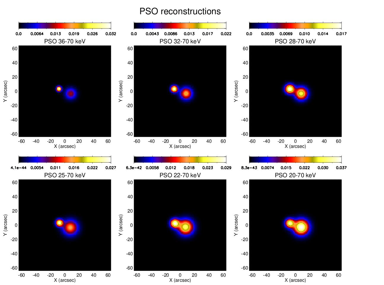
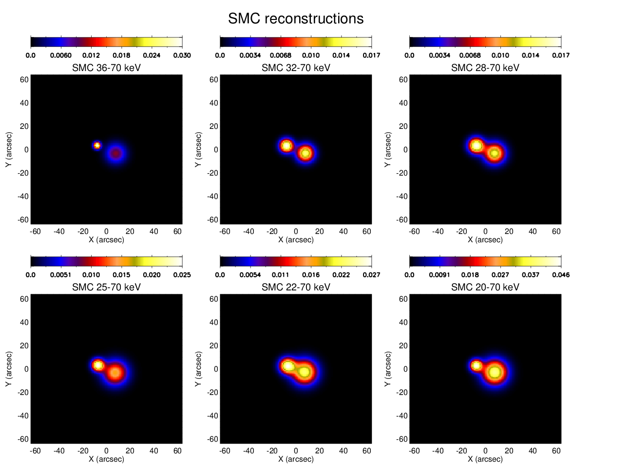
We used PSO and SMC to analyze the visibility amplitudes associated to this flare with the main aim to give a first and very preliminary assessment of STIX imaging performances. Therefore, the results illustrated in the next figures should be intended not as science products but as first hints of what STIX will allow doing for the investigation of hard X-ray flare physics when the instrument calibration process will be completed.
4.1 The 05:45:30 UT – 05:46:15 UT time window
Focusing on the impulsive phase of the flare (05:45:30 UT – 05:46:15 UT), we have applied PSO and SMC to the set of visibility amplitudes corresponding to six energy channels. Each bag was made of visibilities, visibilities being discarded as not yet well-calibrated (the discarded visibilities correspond to detectors with smallest pitch). The reconstruction results are presented in Figure 3, the corresponding fits in Figure 4 and the parameter estimates in Figure 5. The six energy channels have been selected by keeping the upper limit fixed at keV and gradually decreasing the lower limit of the channels. Precisely, we have taken : 36–70 keV, : 32–70 keV, : 28–70 keV, : 25–70 keV, : 22–70 keV and : 20–70 keV, which correspond to the weighted mean energies of keV, keV, keV, keV, keV and keV, respectively. From the spectral analysis, the interval 36–70 keV should mainly contain the nonthermal emission and the corresponding reconstruction presents two distinguished rather compact sources, one at the bottom-right position (first source from now on) and the other one at the up-left position (second source from now on). While decreasing the lower limit of the energy channel, the flux associated to the first source significantly increases, while flux and dimension of the second source remain quite stable. This holds true for the reconstructions provided by both methods and, correspondingly, the small values confirm a notable statistical reliability of the results. A possible interpretation of this behavior is that the first source might be associated to the thermal emission with a nonthermal tail, while the second one reflects a nonthermal bremsstrahlung process. In any case, the interpretation of the physical nature of the different sources is not the goal of this paper, and the interpretation of the hard X-ray sources in this flare is left for when the full calibration of the STIX imaging system is available.


We note that, in the PSO analysis, uncertainty quantification has been performed by means of the confidence strip method, i.e. repeatedly perturbing the input data, re–running the algorithm for each data realization and computing the standard deviations over the set of reconstructed parameters. On the contrary, the SMC method returns the estimated probability distributions of the parameters (via the histograms in Figure 6), and from them, means and standard deviations can be easily computed. This approach, which does not require the perturbation of the data, usually provides smaller uncertainties with respect to the ones provided by the confidence strip approach. The drawback of this method is an higher computational burden with respect to PSO. Indeed, each reconstruction took approximately 5 mins with SMC, while 1.5 mins with the PSO combined with confidence strip. We point out that reconstruction with PSO alone (i.e. not producing uncertainty estimation) is even faster, with 5 sec of computational time.
Another interesting aspect concerning the SMC histograms in Figure 6 is that the width parameters, particularly the ones associated to the second source, are rather narrow. This is rather surprising, given that the six visibilities discarded from the analysis are the ones associated to the smallest angular resolution (smaller than ). However, this super-resolution effect (which is present also in the case of the reconstructions provided by PSO) is a reasonable intrinsic consequence of the application of forward-fitting approaches: indeed, the use of predefined source shapes imposes strong constraints on the solution that may lead to an enhancement of the angular resolution of the reconstruction. This behavior has been noticed also in the case of RHESSI visibilities, when a deterministic forward-fitting approach is applied for parameter estimation (Aschwanden et al. 2002, see point (5) in the Conclusion section of).
Finally, some of the histograms in Figure 6 present a shape that is far from Gaussian-like and is sometimes even close to a bi-modal one. This is most likely due to the fact that we are addressing a very ambiguous problem, in which two configurations characterized by interchanged sources provide the same value. Indeed, visibility amplitudes are not sensitive to parity transformations.
4.2 Time resolution analysis
We considered the STIX observation at 05:46:30 UT of the November 18, 2020, with time integration of one second, in the energy range from to keV, in order to verify whether the count statistic, determined by the count rate recorded by the detectors and measured in counts keV-1 s-1, was sufficient to allow the realization of reliable reconstructions. Figure 7 shows that the count statistic is rather stable across detectors and that even at such a short integration time the statistical error is dominated by the systematic component.
The application of SMC to the corresponding visibility amplitude bag produced the visualization and fitting in Fig. 8, top row, that correspond to an input configuration made of two Gaussian sources. We refer to first source as the most energetic one, and second source as the least energetic one. The histograms for the FWHM and flux parameters in the bottom row of that same figure show that the parameters for both sources are computed with sound uncertainty quantification. The values of such parameters are illustrated in Table 1, where we also reported the results of the analysis performed by means of PSO.


| First source | Second source | |||
|---|---|---|---|---|
| FLUX (counts keV-1 s-1) | FWHM (arcsec) | FLUX (counts keV-1 s-1) | FWHM (arcsec) | |
| SMC | 4055 102 | 16.4 0.4 | 892 213 | 91.8 23.8 |
| PSO | 4120 129 | 16.3 0.5 | 958 295 | 97.8 17.2 |
We note here that the integration time of the November 18, 2020 observation was set to second. This time interval is currently considered as the maximal time resolution achievable by STIX, although tests at faster time cadences (down to 0.1 second) will be carried out later in 2021. Considering our initial results at 1 second cadence, we are confident that sub-second time resolution imaging will be possible at least in the thermal range.
5 Comments and conclusions
This study represents a preliminary attempt to reconstruct hard X-ray images of solar flares from data collected by STIX during its cruise phase. As a consequence, these results should be considered with caution, first of all because the current calibration stage of the instrument does not allow the exploitation of the visibility phases, so that the non–linear image reconstruction problem of determining the flaring source from the visibility amplitudes is highly ambiguous. It follows that the only approaches we could implement were the ones based on the forward fitting of very simple parametric source shapes and the only information we could try and determine were related to the flux and dimensions of such shapes and, in the case of a configuration made of two Gaussian sources, their relative position.
However, even with these limitations, some hints can be deduced from the results of this analysis. For example, STIX seems to allow a high temporal resolution analysis, providing data with significantly high signal–to–noise ratio even in the case of very short integration times. Further, a simple spectral analysis provided us with results that are consistent with a scenario in which a nonthermal footpoint persists at higher energies, while a (probably coronal) thermal component becomes more evident when lower energies are included in the processing.
Finally, the two parametric imaging approaches considered in this work provide rather similar reconstructions. However, from a methodological viewpoint, the two methods have a key difference: PSO realizes uncertainty quantification through the confidence strip method, which is fast but does not leave the measurements untouched, possibly leading to suboptimal results. SMC provides a full probabilistic description of the reconstructed shapes, and therefore a more robust uncertainty estimation, but at the cost of an higher computational burden. We point out that both methods can be easily extended for use with fully calibrated visibilities (i.e., when even the visibility phases will be calibrated) and that they will be included in the STIX data analysis software of the mission.
Acknowledgements.
Solar Orbiter is a space mission of international collaboration between ESA and NASA, operated by ESA. The STIX instrument is an international collaboration between Switzerland, Poland, France, Czech Republic, Germany, Austria, Ireland, and Italy. AFB is supported by the Swiss National Science Foundation Grant 200021L_189180 for STIX. PM, EP, FB and MP acknowledge the financial contribution from the agreement ASI-INAF n.2018-16-HH.0. SG acknowledges the financial support from the ”Accordo ASI/INAF Solar Orbiter: Supporto scientifico per la realizzazione degli strumenti Metis, SWA/DPU e STIX nelle Fasi D-E”.References
- Aschwanden et al. (2002) Aschwanden, M. J., Schmahl, E., & RHESSI Team. 2002, Sol. Phys., 210, 193
- Aschwanden et al. (2003) Aschwanden, M. J., Schmahl, E., & Team, R. 2003, in The Reuven Ramaty High-Energy Solar Spectroscopic Imager (RHESSI) (Springer), 193–211
- Dennis & Pernak (2009) Dennis, B. R. & Pernak, R. L. 2009, ApJ, 698, 2131
- Duval-Poo et al. (2018) Duval-Poo, M. A., Piana, M., & Massone, A. M. 2018, A&A, 615, A59
- Eberhart & Kennedy (1995) Eberhart, R. & Kennedy, J. 1995, in 1995 IEEE Int. Conf. Neural Netw., Vol. 4, 1942–1948
- Giordano et al. (2015) Giordano, S., Pinamonti, N., Piana, M., & Massone, A. M. 2015, SIAM J. Imaging Sci., 8, 1315
- Hurford et al. (2002) Hurford, G., Schmahl, E., Schwartz, R., et al. 2002, Sol. Phys., 210, 61
- Kosugi et al. (1992) Kosugi, T., Sakao, T., Masuda, S., et al. 1992, PASJ, 44, L45
- Krucker et al. (2013) Krucker, S., Christe, S., Glesener, L., et al. 2013, in Society of Photo-Optical Instrumentation Engineers (SPIE) Conference Series, Vol. 8862, Solar Physics and Space Weather Instrumentation V, ed. S. Fineschi & J. Fennelly, 88620R
- Krucker et al. (2020) Krucker, S., Hurford, G. J., Grimm, O., et al. 2020, A&A, 642, A15
- Lin et al. (2002) Lin, R. P., Dennis, B. R., Hurford, G. J., et al. 2002, Sol. Phys., 210, 3
- Massa et al. (2019) Massa, P., Piana, M., Massone, A. M., & Benvenuto, F. 2019, A&A, 624, A130
- Massa et al. (2020) Massa, P., Schwartz, R., Tolbert, A., et al. 2020, ApJ, 894, 46
- MATLAB (R2019b) MATLAB. R2019b, Global Optimization Toolbox, The Mathworks, Inc., Natick, Massfachusetts
- Mezura-Montes & Coello Coello (2011) Mezura-Montes, E. & Coello Coello, C. A. 2011, SWEVO, 1, 173
- Nocedal & Wright (1999) Nocedal, J. & Wright, S. 1999, Numerical Optimization (New York: Springer-Verlag)
- Pearson & Readhead (1984) Pearson, T. J. & Readhead, A. C. S. 1984, ARA&A, 22, 97
- Perracchione et al. (2020) Perracchione, E., Massa, P., Massone, A. M., & Piana, M. 2020, arXiv e-prints, arXiv:2012.14007
- Piana (1994) Piana, M. 1994, A&A, 288, 949
- Qasem & Shamsuddin (2011) Qasem, S. N. & Shamsuddin, S. M. 2011, Appl. Soft Comput., 1427
- Sciacchitano et al. (2019) Sciacchitano, F., Lugaro, S., & Sorrentino, A. 2019, SIAM Journal on Imaging Sciences, 12, 319
- Sciacchitano et al. (2018) Sciacchitano, F., Sorrentino, A., Emslie, A. G., Massone, A., & Piana, M. 2018, ApJ, 862, 68