Bayesian Inference Using the Proximal Mapping:
Uncertainty Quantification Under
Varying Dimensionality
Abstract
In statistical applications, it is common to encounter parameters supported on a varying or unknown dimensional space. Examples include the fused lasso regression, the matrix recovery under an unknown low rank, etc. Despite the ease of obtaining a point estimate via optimization, it is much more challenging to quantify their uncertainty. In the Bayesian framework, a major difficulty is that if assigning the prior associated with a -dimensional measure, then there is zero posterior probability on any lower-dimensional subset with dimension . To avoid this caveat, one needs to choose another dimension-selection prior on , which often involves a highly combinatorial problem. To significantly reduce the modeling burden, we propose a new generative process for the prior: starting from a continuous random variable such as multivariate Gaussian, we transform it into a varying-dimensional space using the proximal mapping. This leads to a large class of new Bayesian models that can directly exploit the popular frequentist regularizations and their algorithms, such as the nuclear norm penalty and the alternating direction method of multipliers, while providing a principled and probabilistic uncertainty estimation. We show that this framework is well justified in the geometric measure theory, and enjoys a convenient posterior computation via the standard Hamiltonian Monte Carlo. We demonstrate its use in the analysis of the dynamic flow network data.
Keywords: Concentration of Lipschitz Functions, Generalized Density, Generalized Projection, Hausdorff Dimension, Non-expansiveness.
1 Introduction
Modern statistical applications often involve data that are high dimensional. To allow signal recovery under a relatively low sample size, one often needs to assume that the parameter in fact lies in/near some lower dimensional space. Commonly used assumptions include sparsity [23, 41, 22, 5], low rank [33, 15], geometric constraints [31, 12], etc. In most cases, the dimensionality is unknown. For example, we usually do not know the exact rank in the low-rank matrix factorization.
Bayesian framework provides a principled way to quantify the uncertainty on those models. A potential caveat is that if the assigned prior is associated with a -dimensional continuous measure, then there is zero posterior probability allocated on any of the lower-dimensional subsets with dimension . Instead, from a generative perspective, one should first choose a discrete prior to select , then generate within the chosen space. For example, the spike-and-slab prior [24] assigns a binomial distribution on as the number of non-zero coefficients in the variable selection problem; the Bayesian adaptive regression spline uses a Poisson prior on the number of knots , which determines the rank of the spline matrix [8]. On the other hand, the discrete prior creates a highly combinatorial problem, and existing estimation methods such as the Reversible-jump Markov chain Monte Carlo [13] are not very efficient to explore the high posterior probability region.
An appealing alternative is to avoid specifying any low-dimensional prior, but to induce a prior for with the measure in yet having the mass concentrated near some low-dimensional sets. Specifically, the key is to re-parameterize the parameter as some transformation of a sparse vector , and then assign simple continuous shrinkage prior on to favor near-zero values. For example, in spline regression, one uses as the sparse weights in the linear combination of some basis functions. In this category, there is a rich literature covering tasks of variable selection [27, 6, 30], matrix decomposition [4, 18], functional data analysis [34], covariance estimation [19, 16], among others.
Clearly, this strategy has its limitations — when we cannot re-parameterize the low-dimensional sets of , the prior specification becomes awkward. This is not uncommon. For example, the fused lasso [39] is a frequentist regularization very popular in the image/signal processing, which assumes sparsity not only in the parameter , but also in the increments between the neighboring elements . Although we could imagine assigning some shrinkage prior on with the corresponding matrix, such a prior is ill-defined: as is not invertible, we cannot compute from ; as resides in the column span of , it has a dimension , which is less than — therefore, the shrinkage prior one blindly assigned would be in fact an incomplete density for a degenerate measure, making it difficult to calibrate the hyper-parameters within and assess the effects of the prior regularization.
Motivated to generalize the Bayesian approaches for handling most of the low-dimensional regularizations (including potentially complicated ones), while avoiding the caveats of having to explicitly specify a discrete prior, we consider a “projection”-style approach. Starting from a continuous prior for with measure in , we transform it into using a special mapping, so that has an induced prior on several low-dimensional sets. The projection idea was previously considered in several cases, such as the mixture of components with different dimensions [28], the isotonic regression [9], monotone curve fitting [20] and more generally, constrained space modeling [32]. Nevertheless, in this article, we explore a much more general transformation known as the proximal mapping — it not only includes common Euclidean projection to a constrained set, but also useful non-projection transformation such as soft-thresholding, nuclear norm control, set expansion, etc. This mapping has been well studied in the optimization literature, with appealing properties that are convenient for canonical Bayesian inference, such as in the concentration of measure and convenient computation via the Hamiltonian Monte Carlo. We will carefully justify this prior via the geometric measure theory and demonstrate the strengths via several examples.
2 Method
2.1 Background on the Proximal Mapping
We first provide a brief review on the proximal mapping and motivate its use as a transformation tool. Let be the parameter of interest in a certain space , with . With another parameter , the proximal mapping is a transform of to :
| (1) |
where is a lower semi-continuous and convex function, and is a scalar as a hyper-parameter. This effectively induces a parameter space:
For an intuitive understanding, the proximal mapping could be viewed as a generalized projection. Given a constrained set , we can choose , the characteristic function of a constrained set taking value if , or if . The mapping becomes , the Euclidean projection of into the set . Furthermore, we can replace with other function for , leading to a wider class of transformation.
Example 1. Soft thresholding Perhaps the most famous example is from lasso [38]. It has a closed-form proximal mapping known as the soft-thresholding operator , with all operations carried out element-wise. The induced parameter space is in fact the union of multiple sets with varying dimensions: , where is some index set and , each is a Euclidean subspace of dimension — conveniently, we do not need to explicitly specify the dimension , since it is automatically induced through the transformation.
This suggests that the proximal mapping can be used as a convenient tool to develop priors on lower-dimension subsets. We now list a few useful proximal mappings in Table 1. In addition, the proximal mapping allows us to easily consider multiple constraints or functions, since the intersection of convex sets and summation of convex functions are still convex. The general form can be computed using the alternative direction of method of multipliers algorithm [3], and we will demonstrate one case in the data application. For example, consider being sparse while constrained in some convex set; this would be challenging to model for conventional approaches due to the lack of reparametrization.
| Space of | Usage | ||
|---|---|---|---|
| , convex set | Projection to a set [See Table 6.1 of [1] for an expanded list] | ||
| , computed element-wise | Sparsity | ||
|
,
positive semi-definite} |
, nuclear norm | , with the singular value decomposition, | Low rank |
| with as the th row | Row / group sparsity | ||
|
with
|
Solvable via the alternating direction method of multipliers |
Fused lasso,
convex clustering | |
|
,
distance to a set |
with
|
Set expansion to |
2.2 Proximal Prior
We now use the above in a Bayesian modeling framework. Suppose we have data generated from a likelihood , where we want to assign a prior on in some space with dimensionality smaller or equal to . We use the following generative process for :
| (2) | ||||
where is a continuous distribution in , such as the non-degenerate Gaussian and we use to denote a generative distribution for .
Here is a convex and lower-semicontinuous function such as those in Table 1. Potentially, could be known up to some other hyper-parameter ; in that case, we denote it by and use as the prior for . For a clear notation, we use bold subscript such as in as a book-keeping index to refer to the variable whose prior is being defined.
It is not hard to see that , as the combination of the convex and a quadratic term, is strictly convex with a unique minimizer. Therefore, each maps to a unique , hence we have a measurable mapping, which means we have a valid prior distribution for using (2). We denote the conditional prior distribution for as , and its marginal distribution as after integrating out and . For convenience, we will refer to either form as a “proximal prior”.
We first show that, a proximal prior can produce a convenient equivalence to a hierarchical prior of first selecting a low-dimensional set and then assigning a conditional density within this set. We denote the space induced by as , and assume that it can be partitioned into , where denotes a -dimensional subset of , and if (this can be achieved even if a higher dimensional set overlaps/contains a lower-dimensional set , we set ). Then the prior kernel (a mix of density and mass functions) evaluated at can be written as:
| (3) |
where and is a conditional density that integrates to over using an appropriate -dimensional integral with respect to some proper measure , denoted by . The integral and measure will be formally defined in the theory section.
Therefore, from a generative view, the above can be understood as first picking a set with probability , then drawing a value within the space of . This includes those corner cases where cannot map to some dimensional sets: that is, for some ’s, we can have .
Accordingly, with the likelihood, the posterior of can be derived as:
| (4) |
where . We assume posterior propriety almost everywhere, such that for all .
The proximal priors simplify these procedures. Using the transformation , for any measurable set ,
where in we mean that contains the Jacobian term in the change-of-variables (details of the Jacobian calculation provided in the theory section). At any given , we can omit the integral and summation, and obtain a remarkably simple posterior density of :
| (5) |
Remark 1
To clarify, although the hierarchical form of provides a nice interpretation to our proximal prior, such an equivalence is not strictly necessary for the proximal modeling framework to work. To be rigorous, the above equivalence requires a few regularity conditions, to be formalized in the theory section.
Therefore, compared to (4), the posterior density (5) is much easier for Bayesian applications. This also suggests a new strategy of “data augmentation using optimization” [instead of marginalization as in [37]] — if we can write the parameter as some proximal mapping from , then we can sample first as an augmented variable; after sampling, we compute and discard the information from .
We now use one example to illustrate the equivalence.


Example 2. Affinely constrained prior under varying rank Suppose we want to assign a prior for in a set of affine constraints where is another parameter, with and the column space of (so that is not empty). Since is not fixed, we do not know the rank of , hence not the dimensionality of . Using the proximal prior with if , otherwise (hence is invariant to any finite value of ), and , we have a closed-form proximal mapping
where is the Moore-Penrose inverse. We illustration this mapping in Figure 1.
The -marginal proximal prior is a discrete mixture over different rank of :
and is the degenerate Gaussian density with mean and covariance , where . Although the summation may not have a closed-form, the weights and conditional density can be tractable in applications.
For illustration, we consider a Bayesian envelope linear regression for multivariate response :
for , each covariate (with ), and the noise ; together from a orthonormal matrix, with a sub-matrix, full rank, and both and positive definite matrices. The regression coefficient matrix is of rank , with unknown. The motivation is that by making in the subspace spanned by the leading eigenvectors of the covariance, is small in magnitude and independent from , leading to a sufficient dimension reduction [7]. For Bayesian inference, [17] proposed to use a matrix-Bingham prior on with a pre-specified , so that it has conjugate forms in a Gibbs sampler for posterior computation. On the other hand, since is in an orthogonal and low-rank space, it is difficult to generalize to other forms of prior such as letting vary.
Using the affine constraint proximal mapping, we can bypass these challenges. We reparameterize , with rank, positive definite, and by a linear constraint . The proximal mapping yields , with the matrix form for . Using matrices , , we rewrite the envelope regression likelihood as
where is the pseudo-determinant. To complete the proximal prior specification, we use and , with their elements iid from N (hence full rank almost surely); then we set , and with and , and the -quantile of . We provide a numerical simulation in the Supplementary Materials.
Focusing on the -marginal prior, we have: 1. the mixture weight , where can be specified as a priori; 2. the conditional density containing
The second line is due to being idempotent , , and . This density is invariant to scaling of .
Remark 2
To clarify, we use the above example (with a relatively simple ) to illustrate the equivalence between the hierarchical specification of and the continuous--and-mapping specification. In general cases, the former may be intractable due to the lack of closed-form, hence motivating the proximal mapping strategy as proposed in this article.
In example 2, if we intuitively compare the two distributions before and after the mapping, it reduces (or at least retains) the distance to the center . The property shown in this example is known as the “non-expansiveness”, which in fact holds for all proximal mappings:
for any in the domain of . This is in particular meaningful for Bayesian inference, as it conveniently controls the concentration of measure for .
Theorem 1
If the data come from a distribution with a fixed parameter , and any , the posterior distributions of and satisfy
In addition, if , then
Using the envelope regression example, we know that
which is a multivariate Gaussian for On the other hand, since we know , we know for any given , with , due to being idempotent and having eigenvalues equal to either or .
2.3 Prior Specification on
In the proximal mapping (1), the hyper-parameter plays an important role, hence we need to carefully choose its prior. To first obtain some intuition, note when , we have if for all , the identity mapping; when , we have . Therefore, as increases, becomes farther away from , hence the distribution gets more “deformed” at a larger . We now formalize this deformation intuition, while relaxing the finite-valuedness of . For conciseness, we postpone all the proofs in the appendix.
Theorem 2 (Monotonicity of deformation in )
For any function with range , if , then .
This result means that we can find a measurement between and to quantify the deformation:
| (6) |
where the expectation is taken with respect to the prior of .
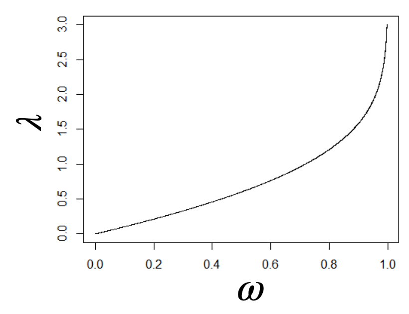
When lacking prior knowledge on , we can use a Beta prior on and solve for :
| (7) |
In this article, we use a non-informative . As a toy example, let be univariate with a finite variance, using the proximal mapping with , we have . Therefore, we have with an induced prior for .
In more general cases, (7) often cannot be solved analytically. However, we can numerically compute a prior for , using a strategy similar to [2] — for chosen points in , we can use the empirical estimates of the expectation based on simulated , and solve for ; afterwards, we can easily interpolate to obtain the associated with any .
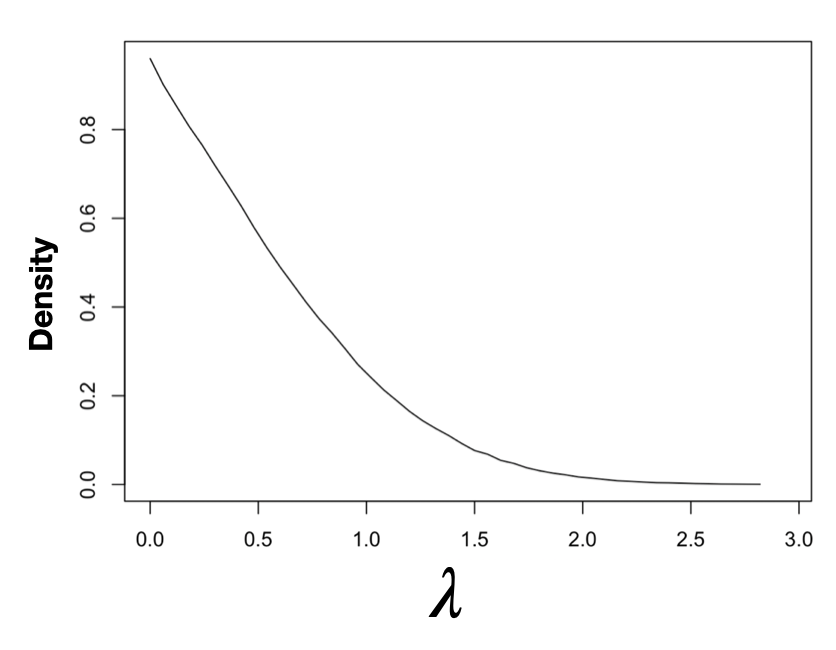
Example 1. (Continued). Soft-thresholding prior To illustrate, we compute the prior of for the soft-thresholding prior based on . Based on and , we compute the prior density of and plot it in Figure 2.
In this section, we discussed the choice of with the generality of all possible and in mind. On the other hand, for some specific case such as and soft-thresholding , there is a connection to some existing prior in the literature, such as the classic spike-and-slab prior. For example, if and to be the -quantile of of , then we can obtain a spike-and-slab prior with Laplace slab . A closely related discovery is the neuronized prior [35] using truncated activation function, for which there is an equivalence to a spike-and-slab prior with two-normal-product slab. In these cases, there are often alternative choices for that are justified via large sample theory. Due to the page constraint, we defer the detailed discussion and numerical experiments to the Supplementary Materials.
3 Geometric Measure Theory on the Varying Dimensional Sets
3.1 Hausdorff Dimension and Low Dimensional Density
We now give a more rigorous exposition on the distribution induced by the proximal mapping. Without loss of generality, we consider as a -element vector. Since may correspond to a measure of a set in the lower dimensional space, the -dimensional Lebesgue measure of any lower-dimensional set is zero hence is not useful. We need some tools from the geometric measure theory to address this issue. To start, consider a set and suppose we do not know its dimensionality. Instead, we can cover with sets ’s, each has its diameter . We call any as a -covering of .
Then we take the infimum over all -coverings of , and letting the decrease, we obtain the -dimensional Hausdorff measure of :
| (8) |
Intuitively, the above can be taken as the minimum total “volume” of the covering — except is a parameter that varies.
In fact, is a non-increasing function in [10]. More importantly, for any Borel , and , if then ; and if then [Theorem 6.1.6 [10]]. This means for any Borel set , there is a unique as a transition point, over which the dimensionality drops from to :
Such an is referred to as the Hausdorff dimension of , equivalently:
| (9) |
Note that does not have to be an integer; nevertheless, when it is, the Hausdorff measure is proportional to the commonly used -dimensional Lebesgue measure
via , where due to the volume formula of an -dimensional ball. In addition, when , is same as the counting measure.
Now recall that is non-expansive, which leads to the following theorem:
Theorem 3
For any Borel set and proximal mapping , we have
- 1.
for any ;
- 2.
.
Remark 3
In the above, the statement 2 is particularly useful: it tells us that only maps to lower or equal dimensional space.
Now, starting from a probability distribution defined by a certain Radon measure in for some low-dimensional sets in , one interesting question is how to differentiate this and obtain a “density”, as used in (3) and (4).
For a point , the ball centered at with radius has the lower and upper -dimensional derivatives:
Therefore, if we have the two limits coincide, we would have a definition of an -dimensional density: , commonly referred to as the -density.
Remark 4
To understand the -density as a generalized concept of “density”, for those continuous distributions associated with a -dimensional Lebesgue measure, such as the non-degenerate Gaussian distribution, the -density is the probability density function; whereas for the discrete distributions, the -density is the same as the probability mass function.
Next, similar to the probability density function, -density may not always exist. Therefore, it is important to state the two required conditions, is an integer and is in a rectifiable set, as formalized in the following theorem.
Theorem 4 (Besicovitch-Marstrand-Preiss theorem)
[29] Let be a locally finite Radon measure on , if there exists a real such that exists, and it is positive on a set of positive -measure, then must be an integer. On the other hand, let be Borel with and an integer, then exists for almost everywhere with respect to , if and only if the set is rectifiable.
To explain “rectifiability”, a Borel set is rectifiable if there is a countable family of Lipschitz maps which cover almost all except for sets with zero measure. That is, intuitively speaking, almost every -element vector can be represented as some transformation of — note that this is not the same as a simple reparameterization, as we may obtain via multiple ’s (up to countably many).
3.2 Calculation of the -Density
We now provide a way to calculate the -density. Focusing on a subset with and . We now transform into an -density with .
Theorem 5
If is -rectifiable and , is -rectifiable and , with , and a.e.-. Then the -density of induced by is
| (10) |
where is the -dimensional Jacobian of at b.
Note that if the low-dimensional set can be reparameterized as a transformation an -element vector, then it is possible to change (10) to an integration with respect to an -dimensional Lebesgue measure.
To explain the assumptions above, a set is -rectifiable when , and there is a set as the countable union of Lipschitz images from bounded sets such that . As the result, if -density exists, we could use (10) when both and are finite.
[25] gives the -dimensional Jacobian of function , differentiable at . Let be the derivative matrix of at , with , , then the -dimensional Jacobian can be computed as:
| (11) |
Note than when , as more commonly seen.
Importantly, by Rademacher’s theorem [11], a Lipschitz function is differentiable almost everywhere. Therefore exists almost surely with respect to . In the following example, we illustrate the use of the above theorem to compute the -density for the affinely constrained prior.
Example 2. The -density of the affinely constrained prior Using (10), one can verify that the -density of affinely constrained prior recovers the “degenerate Gaussian density”. Starting from and let us assume is and , then it is not hard to compute that . Using the proximal mapping, at , we have with , hence we can integrate over the region by re-parameterizing where . Integrating over , we have the -density with :
which is commonly referred to as the “degenerate density” for a degenerate Gaussian, with its covariance having a rank .
We list a few more examples commonly considered in statistics, where for each we have a guaranteed existence of -density: regression under linear equality constraints, matrix factorization under low-rank constraint, sparse regression, covariance modeling in positive-definite space, and directional modeling in orthonormal space.
Remark 5
To clarify, the existence of -density for is not necessary in our modeling framework using proximal mapping, since we can always carry out computation using a valid -dimensional density of . On the other hand, the existence of -density would be required if one wants to interpret the prior via an equivalent prior as in (3).
4 Posterior Computation
As shown in (5), when using instead of , the posterior has a simple density on , and the proximal mapping is differentiable almost everywhere with respect to . Therefore, as long as is a continuous and differentiable function in almost everywhere, we can use the Hamiltonian Monte Carlo (HMC) for posterior computation. Now we first briefly review the HMC algorithm, then address the gradient calculation for the proximal mapping.
To sample from target distribution , the HMC uses an auxiliary momentum variable and samples from a joint distribution , where a common choice of is the density of . Denote and , which are referred to as the potential energy and kinetic energy respectively. The total Hamiltonian energy function is .
At each state , a new state is generated by simulating Hamiltonian dynamics, which satisfies the Hamilton’s equations:
| (12) |
The exact solution for (12) is often intractable, while we can numerically approximate the evolution by algorithms such as the leapfrog scheme. The leapfrog is a reversible and volume-preserving integrator, which updates the evolution via
| (13) |
for , and sets . To correct the numeric error due to approximation, is treated as a proposal and accepted with the Metropolis-Hastings (MH) probability
We now discuss the gradient computation:
When has a closed-form, we can use the automatic differention toolbox to calculate the gradient ; on the other hand, when the closed-form does not exist, some numeric approximation is needed.
Note that the partial gradient is with is the standard basis with the th element equal to one, and all others equal to zero; using a small gives us the finite difference approximation. Nevertheless, when is high dimensional, this would involve times of calculating the proximal mapping, which can be computationally prohibitive. To solve this problem, we follow [36] and use the simultaneous perturbation stochastic approximation:
| (14) |
for , where has each independently generated using . The right hand side is based on the first order approximation to the finite difference form. The advantage is that we only need to evaluate the proximal mapping for times. In this article, we use and and find empirically good stability for the HMC algorithm.
For the HMC as a gradient-based algorithm, another potential concern is that may have zero gradient at certain value of , for example, the soft-thresholding will have zero gradient for those . Fortunately, two things prevent such a from being stuck at a certain value. First, although the log-likelihood may have a zero gradient for , the log-prior does not (as it does not depend on ) — in those cases, will be updated through its prior distribution, until it enters the region where is no longer invariant in . This behavior is quite similar to the one with augmented “continuous particle” for sampling binary distribution via HMC [26], where they demonstrated excellent mixing of Markov chains. Second, the HMC preserves the joint density of (with the MH correction), and as we sample a new at the start of each iteration, the effective range of to reach is , with the mode of . Therefore, as long as , we can have , and allowing to move away from a local-optimal state. In practice, we use the No-U-Turn algorithm [14], which ensures that we run the dynamics for long enough, so that the new proposal is away from the current sate. We provide some diagnostic plots in the Supplementary Materials.
5 Simulation Studies
5.1 Set Expansion Prior for Hypothesis Testing
We now demonstrate the usefulness of the proximal prior in standard statistical inference, such as the hypothesis testing of whether is in a constrained set . Consider two hypotheses and , where For testing, one typically assumes a mixture prior
| (15) |
where and are the prior kernel function of under and , respectively; and is the prior probability assigned to . The Bayes factor of relative to is defined as
for which, a smaller value of provides stronger evidence against . Often, is not of the same dimension with . For example, when testing a point null hypothesis , we have . The standard practice has been assigning appropriate under (and under ), with and being 0 on and respectively. However, when the null hypothesis is low-dimensional, such as testing linear equality, assigning density supported on the null set can become quite challenging.


For a convex null set , we could define a proximal prior based on the distance function, such that the prior density is positive on both and . The distance function from point to set is defined as . The proximal mapping of the distance function to set is of the form
Clearly, this proximal mapping projects the points in the -neighborhood of into , and keeps the rest of the points out of . Thus we get a prior that puts positive mass on both and and can also be expressed in the form of (15).
We can easily estimate the Bayes factor
via posterior sampling methods. If the prior ratio is not specified, in order to obtain adequate number of samples in both and , we can choose a fixed (instead of assigning a prior on ) such that .
We conduct a simulated experiment: we have data generated from with . We want to test the linear equality hypothesis against . The null set is a hyperplane with Hausdorff dimension 2. We assign the set expansion prior to by assign to and set with , such that the prior ratio of and is around Posterior sampling is implemented with the HMC with 5000 samples and 2000 burn-ins. We get an estimated Bayes factor , and display 100 of the samples in Figure 3, panel (b).
5.2 Numerical Experiments on Variable Selection and Low Rank Matrix Model
In addition, we conduct numerical experiments for two models where solutions exist with conventional sparse priors: variable selection using a spike-and-slab prior, and low-rank matrix factorization with a discrete prior on the rank. We compare the computational performance in the combinatorial search-based MCMC algorithms for these models, with the HMC algorithm for our models using proximal priors. Further, we compare with other alternatives such as neuronized prior [35] and multiplicative shrinkage prior [4, 18]. We provide the details in the Supplementary Materials.
6 Data Application: Interpretable Factor Analysis of the Flow Network
We now demonstrate the practical usefulness of the proximal prior via analyzing the dynamic flow network data. The data [42] include dynamic estimated traffic flow on major roads in Florida every 6 hours before Hurricane Irma made landfall until it covered the entire state (between 18:00 on September/6/2017 and 18:00 on September/11/2017). In total, the data contain 25 valid temporal records of flow networks, denoted by ; each contains the traffic flows during a 6-hour period on the roads between urban regions.
Each flow network is a weighted graph , with the set of nodes, the edges, and the weight , representing the amount of flow between the two nodes, with a flow , and a flow . On the diagonal, indicates an external in-flow entering the network, while means an exiting out-flow; if .
To find useful patterns underneath the raw observation data, we use a low-dimensional latent factor model, with the factors shared by all time points, while letting the loadings vary over time, subject to Gaussian measurement error for .
| (16) |


Now, to make the factors useful in interpretation, we require each to be a feasible flow — an idealized flow network satisfying the following constraints, (i) skew-symmetry (except for the diagonal): for ; (ii) flow-conservation, that the net sum of in-flows should equal to the out-flows for node , ; (iii) to reduce noise, we assume that the elements of are sparse. Further, as we expect that most of the nodes do not have an external in-low/out-flow, we assume that (iv) most of the nodes having . To obtain the parameter in such a highly constrained space, we use the proximal mapping, with ,
| (17) | ||||
The proximal mapping does not have a closed-form solution, however, can be efficiently computed using the the alternating direction method of multipliers. Note that with constraint (i) and (ii), it is sufficient to use the lower-triangular entries to represent the rest. In the following, we use to denote the vector containing the lower-triangular entries. Therefore (17) is equivalent to
| (18) |
This proximal operator is evaluated via the alternating direction method of multipliers and solved iteratively. We provide the detailed algorithm in the appendix.
On the prior of the loading, we assign a group shrinkage prior by using the -matrix norm in the proximal mapping. For the matrix , we set:
where . This prior has the advantage that will be simultaneously zero for certain — which allows us to use an overfitted model with a relatively large , with the posterior recovering only a small number of factors with non-zero loadings. We use independent standard normal as prior on the elements of and .
We run the HMC for 20,000 steps and discard the first 5,000 as burn-ins, and we use thinning at every 10th iteration as the posterior sample. The posterior shows the highest probability at having factors, and we visualize them in Figure 4(d) — clearly, by forcing the external in-flows and out-flows to be sparse, we have each factor roughly corresponding to a single connected sub-network.
Interestingly, examining the estimated loadings that change over the time points in Figure 4(c), we see that in the beginning of the evacuation, the factors 1 and 2 are dominant, but later there is a sudden decrease — this in fact corresponds to the time point when the hurricane makes the landfall, effectively forcing the traffic in those areas to shut down. After the 60th hour, the traffic moves up to the north part, and factor 3 represents the late stage of the evacuation.
To compare, we also test two continuous shrinkage priors on the factors. Specifically, we use (a) the elementwise horseshoe prior on each lower-diagonal , , , and (b) the two-way group horseshoe prior, by letting , , . The purpose of (b) is to shrink each row of simultaneously, while satisfying the skew-symmetry of . Effectively these horseshoe priors accommodate the properties of (i)(ii)(iii) of a sparse feasible flow, nevertheless, they cannot accommodate (iv) — as each is completely determined given , we could not further assign shrinkage prior on . As the result in Figure 4(f), the elementwise continuous shrinkage priors show a large number of external in-flows and out-flows, leading to fragmented small networks in each factor. As shown in Figure 4(g), the two-way group horseshoe finds many nodes with no flows at all, which is not very interpretable since we would like most of the nodes to have many in-flows and out-flows, as long as the total net-flow is zero.
7 Discussion
In this article, we exploit the proximal mapping to produce a new class of priors. As we have demonstrated, these priors and the associated probabilistic models can enable statistical inference (such as uncertainty quantification, hypothesis testing) on a wide range of problems, where in the past, one has been limited to point estimate only. The technique of “data augmentation using optimization” we have introduced could be generalized for other purposes, such as potentially new efficient algorithm for the posterior computation. Lastly, one could consider other type of optimization problems for a similar prior construction, such as the popular classes of semi-definite [40] and / or mixed integer programmings [21], although how to provide a probabilistic treatment for these problems is still an open question.
Appendix A Appendix
A.1 Proof of Theorem 1
Proof:
For any value using at given and , . Therefore, Taking the minimum over on the right hand side and expectation on both sides, we obtain the first result.
Next, using the fact that for two independent copies , from , and the non-expansiveness of proximal mappings, we obtain the second result.
A.2 Proof of Theorem 2
Proof:
Let , and we prove: (i) and (ii) For (i),
where is due to is the minimizer of , and similarly for in . Therefore, , which leads to
For (ii), slightly changing (a), we have Since , we have .
A.3 Proof of Theorem 3
Proof:
Since the proximal mapping satisfies -Lipschitz condition, for all in the domain of . Using the definition of the Hausdorff measure, . To see the statement 2, we apply the result in statement 1 and see whenever .
A.4 Proof of Theorem 5
Proof:
Using Theorem 3.2.22 of [11], for any measurable function on ,
Using the assumption, we can exclude the zero-measure set where .
A.5 Algorithm to Compute the Proximal Mapping in the Flow Network Modeling
We formulate an equivalent problem to (18)
| (19) | ||||
where is the matrix such that . The scaled augmented Lagrangian for (19) is:
In each iteration we update the and separately to minimize the Lagrangian:
and update as in dual ascent:
until convergence (i.e., ).
References
- [1] Amir Beck. First-order Methods in Optimization. SIAM, 2017.
- [2] James O Berger, José M Bernardo, Dongchu Sun, et al. The Formal Definition of Reference Priors. Annals of Statistics, 37(2):905–938, 2009.
- [3] Dimitri P Bertsekas. Constrained Optimization and Lagrange Multiplier Methods. Academic press, 2014.
- [4] Anirban Bhattacharya and David B Dunson. Sparse Bayesian Infinite Factor Models. Biometrika, pages 291–306, 2011.
- [5] Peter J. Bickel, Ya’acov Ritov, and Alexandre B. Tsybakov. Simultaneous Analysis of Lasso and Dantzig Selector. The Annals of Statistics, 37(4):1705–1732, 2009.
- [6] Carlos M. Carvalho, Nicholas G. Polson, and James G. Scott. Handling Sparsity via the Horseshoe. In Artificial Intelligence and Statistics, pages 73–80, 2009.
- [7] R Dennis Cook, Bing Li, and Francesca Chiaromonte. Envelope Models for Parsimonious and Efficient Multivariate Linear Regression. Statistica Sinica, pages 927–960, 2010.
- [8] Ilaria DiMatteo, Christopher R Genovese, and Robert E Kass. Bayesian Curve-Fitting With Free-Knot Splines. Biometrika, 88(4):1055–1071, 2001.
- [9] David B. Dunson and Brian Neelon. Bayesian Inference on Order-constrained Parameters in Generalized Linear Models. Biometrics, 59(2):286–295, 2003.
- [10] Gerald Edgar. Measure, Topology, and Fractal Geometry. Springer Science & Business Media, 2007.
- [11] Herbert Federer. Geometric Measure Theory. Springer, 2014.
- [12] Colin R. Goodall and Kanti V. Mardia. Projective Shape Analysis. Journal of Computational and Graphical Statistics, 8(2):143–168, 1999.
- [13] Peter J Green and David I Hastie. Reversible Jump MCMC. Genetics, 155(3):1391–1403, 2009.
- [14] Matthew D Hoffman, Andrew Gelman, et al. The No-U-Turn Sampler: Adaptively Setting Path Lengths in Hamiltonian Monte Carlo. Journal of Machine Learning Research, 15(1):1593–1623, 2014.
- [15] Hui Ji, Chaoqiang Liu, Zuowei Shen, and Yuhong Xu. Robust Video Denoising using Low Rank Matrix Completion. In 2010 IEEE Computer Society Conference on Computer Vision and Pattern Recognition, pages 1791–1798. IEEE, 2010.
- [16] Gregor Kastner. Sparse Bayesian Time-Varying Covariance Estimation in Many Dimensions. Journal of Econometrics, 210(1):98–115, 2019.
- [17] Kshitij Khare, Subhadip Pal, and Zhihua Su. A Bayesian Approach for Envelope Models. The Annals of Statistics, pages 196–222, 2017.
- [18] Sirio Legramanti, Daniele Durante, and David B Dunson. Bayesian Cumulative Shrinkage for Infinite Factorizations. Biometrika, 107(3):745–752, 2020.
- [19] Yunfan Li, Bruce A Craig, and Anindya Bhadra. The Graphical Horseshoe Estimator for Inverse Covariance Matrices. Journal of Computational and Graphical Statistics, 28(3):747–757, 2019.
- [20] Lizhen Lin and David B. Dunson. Bayesian Monotone Regression Using Gaussian Process Projection. Biometrika, 101(2):303–317, 2014.
- [21] Jeff T Linderoth and Martin WP Savelsbergh. A Computational Study of Search Strategies for Mixed Integer Programming. INFORMS Journal on Computing, 11(2):173–187, 1999.
- [22] Lukas Meier, Sara Van De Geer, and Peter Bühlmann. The Group Lasso for Logistic Regression. Journal of the Royal Statistical Society: Series B (Statistical Methodology), 70(1):53–71, 2008.
- [23] Nicolai Meinshausen and Peter Bühlmann. High-dimensional Graphs and Variable Selection with the Lasso. The Annals of Statistics, 34(3):1436–1462, 2006.
- [24] Toby J. Mitchell and John J. Beauchamp. Bayesian Variable Selection in Linear Regression. Journal of the American Statistical Association, 83(404):1023–1032, 1988.
- [25] Frank Morgan. Geometric Measure Theory: a Beginner’s Guide. Academic Press, 2016.
- [26] Ari Pakman and Liam Paninski. Auxiliary-variable exact Hamiltonian Monte Carlo samplers for binary distributions. Advances in Neural Information Processing Systems, 26, 2013.
- [27] Trevor Park and George Casella. The Bayesian Lasso. Journal of the American Statistical Association, 103(482):681–686, 2008.
- [28] Giovanni Petris and Luca Tardella. A Geometric Approach to Transdimensional Markov chain Monte Carlo. Canadian Journal of Statistics, 31(4):469–482, 2003.
- [29] David Preiss. Geometry of Measures in Rn: Distribution, Rectifiability, and Densities. Annals of Mathematics, pages 537–643, 1987.
- [30] Veronika Rockova and Edward I George. The Spike-And-Slab Lasso. Journal of the American Statistical Association, 113(521):431–444, 2018.
- [31] Olli Saarela and Elja Arjas. A Method for Bayesian Monotonic Multiple Regression. Scandinavian Journal of Statistics, 38(3):499–513, 2011.
- [32] Deborshee Sen, Sayan Patra, and David B. Dunson. Constrained Bayesian Inference through Posterior Projections. arXiv preprint arXiv:1812.05741, 2018.
- [33] Haipeng Shen and Jianhua Z. Huang. Sparse Principal Component Analysis via Regularized Low Rank Matrix Approximation. Journal of Multivariate Analysis, 99(6):1015–1034, 2008.
- [34] Minsuk Shin, Anirban Bhattacharya, and Valen E Johnson. Functional Horseshoe Priors for Subspace Shrinkage. Journal of the American Statistical Association, 115(532):1784–1797, 2020.
- [35] Minsuk Shin and Jun S Liu. Neuronized Priors for Bayesian Sparse Linear Regression. Journal of the American Statistical Association, pages 1–16, 2021.
- [36] James C Spall et al. Multivariate stochastic approximation using a simultaneous perturbation gradient approximation. IEEE Transactions on Automatic Control, 37(3):332–341, 1992.
- [37] Martin A Tanner and Wing Hung Wong. The Calculation of Posterior Distributions by Data Augmentation. Journal of the American Statistical Association, 82(398):528–540, 1987.
- [38] Robert Tibshirani. Regression Shrinkage and Selection via the Lasso. Journal of the Royal Statistical Society: Series B (Methodological), 58(1):267–288, 1996.
- [39] Robert Tibshirani, Michael Saunders, Saharon Rosset, Ji Zhu, and Keith Knight. Sparsity and Smoothness via the Fused Lasso. Journal of the Royal Statistical Society: Series B (Statistical Methodology), 67(1):91–108, 2005.
- [40] Lieven Vandenberghe and Stephen Boyd. Semidefinite Programming. SIAM review, 38(1):49–95, 1996.
- [41] Peng Zhao, Guilherme Rocha, and Bin Yu. Grouped and Hierarchical Model Selection through Composite Absolute Penalties. Department of Statistics, UC Berkeley, Tech. Rep, 703, 2006.
- [42] Yi-Jie Zhu, Yujie Hu, and Jennifer M Collins. Estimating Road Network Accessibility During a Hurricane Evacuation: A Case Study of Hurricane Irma in Florida. Transportation Research Part D: Transport and Environment, 83:102334, 2020.