Algorithm Engineering for Cut Problems
Abstract
Graphs are a natural representation of data from various contexts, such as social connections, the web, road networks, and many more. In the last decades, many of these networks have become enormous, requiring efficient algorithms to cut networks into smaller, more readily comprehensible blocks. In this work, we aim to partition the vertices of a graph into multiple blocks while minimizing the number of edges that connect different blocks. There is a multitude of cut or partitioning problems that have been the focus of research for multiple decades. This work develops highly-efficient algorithms for the (global) minimum cut problem, the balanced graph partitioning problem and the multiterminal cut problem. All of these algorithms are efficient in practice and freely available for use11 1 https://github.com/VieCut/VieCut. In particular, we obtain the following results and algorithms:
- •
Fast heuristic and exact shared-memory parallel algorithms for the (global) minimum cut problem. We present efficient implementations of existing techniques and combine them with novel approaches to give algorithms that find a minimum cut in huge networks significantly faster than state-of-the-art algorithms. Our heuristic algorithm has a lower empirically observed error rate than existing inexact algorithms for the problem.
- •
The first engineered algorithm that finds all (global) minimum cuts and returns a compact cactus graph data structure which represents all of them in graphs with billions of edges in a few minutes. With a multitude of data reduction techniques, we improve the running time of state-of-the-art algorithms by up to multiple orders of magnitude. Based on the representation of all minimum cuts, we are able to find the most balanced minimum cut in time linear to the size of the cactus graph.
- •
A fully-dynamic minimum cut algorithm that efficiently maintains the minimum cut on a graph under edge insertions and deletions. While there is theoretical work, our algorithm is the first implementation of a fully-dynamic algorithm for the problem. Our algorithm uses the theoretical foundation and builds on it with efficient and finely-tuned implementations to give an algorithm that gives up to multiple orders of magnitude speedup to static recomputation.
- •
An integer linear programming (ILP) based meta-heuristic for the balanced graph partitioning problem. As ILPs do not scale to large inputs, we define a much smaller model that allows us to use symmetry breaking and make the approach more scalable. This gives a powerful local search meta-heuristic that can improve given high-quality partitionings even further. We incorporate this meta-heuristic into an existing evolutionary algorithm to give an algorithm that computes state-of-the-art partitionings from scratch.
- •
A shared-memory parallel exact branch-and-reduce algorithm for the multiterminal cut problem. For this algorithm, we develop and engineer highly-efficient data reduction rules to transform a problem into a much smaller equivalent problem. Additionally we give an inexact algorithm that gives high-quality solutions for very hard problems in reasonable time.
Abstract
Graphen sind eine natürliche Representation von Daten aus zahlreichen Kontexten, zum Beispiel Verbindungen in sozialen Netzwerken, Web-Netzwerken, Straßennetzwerken und vielen weiteren. In den letzten Jahrzehnten sind viele dieser Netzwerke zu enormer Größe gewachsen, was effiziente Algorithmen zu ihrer Partitionierung in kleinere, eher begreifliche Teile erforderlich macht. In dieser Arbeit versuchen wir, die Knoten von Graphen in mehrere Blöcke zu partitionieren, so dass die Anzahl von Kanten, welche Blockgrenzen schneiden, minimiert wird. Es gibt eine Vielzahl von Schnitt- und Partitionierungsproblemen auf Graphen, welche Bereits seit Jahrzehnten erforscht werden. Diese Arbeit entwickelt hocheffiziente Algorithmen für das (Global) Minimum Cut Problem, das Balanced Graph Partitioning Problem und das Multiterminal Cut Problem. Alle hierbei entwickelten Algorithmen sind effizient in der Praxis und frei nutzbar22 2 https://github.com/VieCut/VieCut. Im Einzelnen haben wir die folgenden Ergebnisse erzielt und Algorithmen entwickelt:
- •
Schnelle heuristische und exakte shared-memory parallele Algorithmen für das (Global) Minimum Cut Problem. Wir präsentieren effiziente Implementierungen bestehender Methoden und kombinieren diese mit neuartigen Verfahren, um Algorithmen zu entwickeln, die einen minimalen Schnitt signifikant schneller finden können als der bisherige Stand der Forschung. Die heuristische Variante unseres Algorithmus hat hierbei auch eine deutlich niedrigere empirisch beobachtete Fehlerrate als bestehende inexakte Algorithmen für das Problem.
- •
Der erste praktisch effiziente Algorithmus, welcher alle global minimalen Schnitte eines Graphen findet und eine kompakte Cactus Graph Datenstruktur bildet, welche diese Schnitte repräsentiert. Unser Algorithmus findet alle minimalen Schnitte in Graphen mit bis zu mehreren Milliarden Kanten und mehreren Millionen minimalen Schnitten in wenigen Minuten. Mithilfe einer Vielzahl von Datenreduktionstechniken verbessern wir die Laufzeit von bestehenden Algorithmen um bis zu mehreren Größenordnungen. Ausgehend von der Cactus Graph Repräsentation sind wir auch in der Lage, den Most Balanced Minimum Cut in Laufzeit linear zur Größe des Kaktusgraphen zu finden.
- •
Ein fully-dynamic Minimum Cut Algorithmus, welcher effizient einen minimalen Schnitt eines Graphen unter Kanteneinfügungen und -löschungen aufrecht erhält. Während es bereits theoretische Forschung zu diesem Problem gibt, ist unser Algorithmus der erste implementierte fully-dynamic Algorithmus für das Problem. Unsere Arbeit nutzt die bestehenden theoretischen Grundlagen und kombiniert sie mit effizienten und fein abgestimmten Implementierungen, um zu einem Algorithmus zu gelangen, welcher um bis zu mehrere Größenordnungen schneller ist als Neuberechnung mit statischen Algorithmen.
- •
Eine Metaheuristik auf Basis von ganzzahliger linearer Optimierung für das Balanced Graph Partitioning Problem. Da ganzzahlige lineare Programme nicht für große Eingaben skalieren, definieren wir ein deutlich kleineres Modell, auf welchem wir das Problem unter Zuhilfenahme von Symmetry Breaking skalierbar machen. Dies resultiert in einer mächtigen Metaheuristik zur lokalen Suche, welche existierende hochqualitative Partitionierungen noch weiter verbessern kann. Wir binden diese Metaheuristik in einen existierenden evolutionären Algorithmus ein und erhalten so einen Algorithmus, der Partitionierung hoher Qualität selbst erzeugen kann.
- •
Ein shared-memory paralleler exakter Algorithmus für das Multiterminal Cut Problem. Für diesen branch-and-reduce Algorithmus entwickeln wir hocheffiziente Datenreduktionsregeln, um ein Problem in ein viel kleineres äquivalentes Problem umzuwandeln. Außerdem präsentieren wir einen inexakten Algorithmus, welcher hochqualitative Lösungen für extrem schwere Instanzen in annehmbarer Zeit liefert.
Acknowledgments
Thank you to everyone who made these last four years a very enjoyable time - I learned a lot and got to explore very interesting problems!
First and foremost, I would like to thank my advisors Monika Henzinger and Christian Schulz for their support and guidance with my research. You gave me many opportunities to learn new things and approach fascinating problems. Thank you for being so incredibly generous with your time and expertise!
Also, I would like to thank Darren Strash for great collaboration on the papers we wrote together! Thank you also to Ulrich Meyer and Ulrik Brandes who agreed to review this thesis. I could not have wished for a better thesis committee.
I am deeply thankful to Andrew Goldberg for providing me with the incredible opportunity to do an internship at Amazon. On this note, I am very thankful to Quico Spaen, Nhat Le, Larissa Petroianu, Mauricio Resende, Tim Jacobs, and many others for making this internship memorable and enjoyable. I learned so much from all of you!
Being a part of the TAA research group over the past few years has been a great experience! I want to thank Stefan Neumann, Gramoz Goranci, Bernhard Schuster, Alexander Svozil, Marcelo Fonseca Faraj, Wolfgang Ost, and Richard Paul for being great office mates! Thank you to Stefan, Alexander, and Gramoz for helping me find my way in the wonderful city of Vienna; and to Marcelo and Wolfgang for many fruitful discussions. I would also like to thank Sebastian Forster, Kathrin Hanauer, Rudolf Hürner, Sagar Kale, Shahbaz Khan, Ami Paz, Pan Peng, Xiaowei Wu, Vaidehi Srinivas, Ulrike Frolik-Steffan, Iris Gundacker, and Christina Licayan for being wonderful colleagues and making these years very enjoyable!
I am very grateful to my friends and family for their endless support during my years of university and graduate school. I thank my parents Birgitt and Wolfgang for always being there for me.
Finally, I would like to wholeheartedly thank my partner Anique-Marie Cabardos for her love and support. Thank you for keeping me happy and motivated and thank you for your valuable help with proofreading manuscripts and parts of this thesis!
The research leading to these results has received funding from the European Research Council under the European Community’s Seventh Framework Programme (FP7/2007-2013) /ERC grant agreement No. 340506.
Partially supported by DFG grant SCHU 2567/1-2.
Moreover, we gratefully acknowledge the Gauss Centre for Supercomputing e.V. (www.gauss-centre.eu) for funding this project by providing computing time on the GCS Supercomputer SuperMUC at Leibniz Supercomputing Centre (www.lrz.de).
We further thank the Vienna Scientific Cluster (VSC) for providing high performance computing resources.
Bibliographic Note
Several results in this thesis were already published in conference and journal papers and thus the chapters of this thesis are based on the following papers:
- •
Chapter 3: Monika Henzinger, Alexander Noe, Christian Schulz and Darren Strash. “Practical Minimum Cut Algorithms”. In: ALENEX., 2018, pp. 48–61
https://arxiv.org/abs/1708.06127
Monika Henzinger, Alexander Noe, Christian Schulz and Darren Strash “Practical Minimum Cut Algorithms”. In: ACM JEA., 2018, Vol. 23, Article 1.8 pp. 1-22
https://doi.org/10.1145/3274662 - •
Chapter 4: Monika Henzinger, Alexander Noe and Christian Schulz. “Shared-memory Exact Minimum Cuts”. In: IPDPS., 2019., pp. 13–22
https://arxiv.org/abs/1808.05458 - •
Chapter 5: Monika Henzinger, Alexander Noe, Christian Schulz and Darren Strash. “Finding All Global Minimum Cuts in Practice”. In ESA., 2020., Article 59, pp. 1–20
https://arxiv.org/abs/2002.06948 - •
Chapter 6: Monika Henzinger, Alexander Noe and Christian Schulz. “Practical Fully Dynamic Minimum Cut Algorithms”. Manuscript., 2021.
https://arxiv.org/abs/2101.05033 - •
Chapter 7: Alexandra Henzinger, Alexander Noe and Christian Schulz. “ILP-based Local Search for Graph Partitioning”. In: SEA., 2018., Article 4, pp. 1–15
https://arxiv.org/abs/1802.07144
Alexandra Henzinger, Alexander Noe and Christian Schulz. “ILP-based Local Search for Graph Partitioning”. In: ACM JEA., 2020., Vol. 25, Article 9, pp. 1–26
https://doi.org/10.1145/3398634 - •
Chapter 8: Monika Henzinger, Alexander Noe and Christian Schulz. “Shared-memory Branch-and-reduce for Multiterminal Cuts”. In: ALENEX., 2020., pp. 42–55
https://arxiv.org/abs/1908.04141
Monika Henzinger, Alexander Noe and Christian Schulz. “Faster Parallel Multiterminal Cuts”, Manuscript., 2020.
https://arxiv.org/abs/2004.11666
Authors appear in alphabetical order in all listed publications.
veelo \setsecnumdepthsubsection \settocdepthsubsection
titlepage \makeoddheadtitlepage
adjustwidth*-
Dissertation / Doctoral Thesis
Titel der Dissertation / Title of the Doctoral Thesis
verfasst von / submitted by
\theauthor
angestrebter akademischer Grad / in partial fulfillment of the
requirement for the degree of
Doktor der Technischen Wissenschaften (Dr. techn.)
| Wien, 2021 / Vienna, 2021 | |
| Studienkennzahl lt. Studienblatt: / | |
| degree programme code as it appears on the student | |
| record sheet: | A 786 880 |
| Dissertationsgebiet lt. Studienblatt: / | |
| field of study as it appears on the student record sheet: | Informatik |
| Betreuerin: / Supervisor: | Univ.-Prof. Dr. Monika Henzinger |
*
Chapter 0 Introduction
1 Motivation
In the last few decades, world-spanning networks have created a plethora of structured and unstructured data. One very prominent example is the internet, which has seen the creation and growth of many networks, some of them to immense scale. This immense scale makes extracting information from the networks a hard task and necessitates the partitioning of networks into smaller, more readily comprehensible blocks. Graphs are a good abstraction to constitute such networks in a way that is understandable both for humans and machines. In a graph, we have a set of vertices, where each vertex represents an entity, such as a person, street address or a work package in a computer program. If two vertices are linked, such as friends in a social network or street addresses that are connected by a road, they are connected by an edge. This work focuses on undirected graphs, i.e. edges do not have a direction and a connection from A to B implies that B is also connected to A. In some graphs, vertices and edges have weights, for example if we have a graph that depicts a complex program where vertices are subprograms and connections represent communication, vertex weights indicate the computational complexity of a subprogram and edge weights indicate communication volume.
Graph algorithms aim to solve problems on such a graph. In this work, we look at various cut problems or partitioning problems, problems in which we want to partition the set of vertices into two or more subsets. Due to the large scale of global connections we want to be able to partition them into more manageable subgraphs. In all of the problems discussed in this dissertation, we aim to partition the set of vertices in such a way that the total weight of cut edges, i.e. edges that connect vertices in different blocks, or number of cut edges in graphs without edge weights, is minimized. We call the weight sum of cut edges the cut size. This allows the partitioning of networks in such a way that communication over block boundaries in computing networks or separated relationships in social networks is as small as possible.
In this dissertation, we look at three important cut problems. In Part 1 we look at the minimum cut problem or global minimum cut problem where the aim is to find the smallest cut between two non-empty blocks of vertices without making any restrictions on the size of either block. In Part 2, we look at the balanced graph partitioning problem. In this problem we aim to partition the vertex set into blocks of roughly equal size so that the cut size is minimal. Part 3 deals with the multiterminal cut problem, where, given a set of vertices called terminals, we want to find the smallest cut that pairwisely separates all terminals. The three parts of the dissertation are mostly independent; however, some techniques and ideas are shared between algorithms for different problems. We then give a brief re-introduction in the latter part and also cross-reference to the previous usage for further details.
We use the methodology and techniques of algorithm engineering [164] to give algorithms which give fast and strong solutions on a wide variety of different real-world instances but also stand on a sound theoretical base. In the methodology of algorithm engineering, algorithms are designed and analyzed using realistic machine models. In contrast to algorithm theory, these algorithms are then implemented and evaluated using experiments on data from real-world applications. Based on these experiments, we amend our design and repeat this inductive cycle until our algorithm is satisfactory. One important aspect is that the results of the implementation can be published as algorithm libraries so that other people can use them. As we develop algorithms for fundamental graph problems in this dissertation, we publish all of our algorithms under the permissive MIT license so that they can be used as building blocks for complex systems. The implementations in Parts 1 and 3 are available as the VieCut (Vienna Minimum Cuts) library 33 3 https://github.com/VieCut/VieCut, the implementations in Part 2 are integrated into the KaHIP 44 4 https://github.com/KaHIP/KaHIP graph partitioning framework [163, 161]. For a detailed description of the methodology of algorithm engineering we refer the reader to [164].
For the minimum cut problem and the multiterminal cut problem, we develop and use a multitude of local reduction rules or kernelization rules. These reduction rules are related to the concept of fixed-parameter tractable (FPT) algorithms, where a hard problem can be solved efficiently as long as some problem parameter is not too large. FPT algorithms have long been a well-established field in algorithm theory, however only few of the techniques are implemented and tested on real datasets, and their practical potential is far from understood. More recently, the engineering aspect has gained some momentum. There are several experimental studies in this area that take up ideas from FPT or kernelization theory, e.g. for independent sets (or equivalently vertex cover) [27, 35, 44, 122, 97, 98], for cut tree construction[5], for treewidth computations [16, 183, 117], for the feedback vertex set problem [114, 62], for the dominating set problem [2], for the maximum cut problem [57], for the cluster editing problem [23], and the matching problem [116]. In this dissertation, we make heavy use of data reduction techniques to improve the performance of algorithms for the minimum cut problem and the multiterminal cut problem. A recent survey on data reduction rules in practice is given in [1]. This survey covers data reduction for the global minimum cut problem and the multiterminal cut problem, as well as a multitude of other problems.
2 Main Contributions and Outline
This thesis consists of three individual parts, each addressing a fundamental cut problem. In this section, we give a brief overview where we briefly introduce the problems and then give the main contributions in this dissertation. In the introductory sections or chapters of each part we will give a more detailed outline.
1 Part I: Minimum Cut
In the first part of this dissertation we study the (global) minimum cut problem. This part is larger than the others, as we give inexact and exact shared-memory parallel algorithms for the problem, as well as an algorithm that finds all minimum cuts and an algorithm that maintains a minimum cut on a dynamically changing graph in which edges are inserted and deleted in arbitrary order. The minimum cut problem on a graph is to partition the vertices into two non-empty sets so that the sum of edge weights between the two sets is minimized. The minimum cut problem is one of the most fundamental graph problems and has seen a large amount of research. In Chapter 1, we give a brief overview over this research and introduce in a bit more detail algorithms that we use in the following chapters. We first give a practical shared-memory parallel heuristic algorithm in Chapter 2. This algorithm repeatedly reduces the input graph size with both heuristic and exact techniques by identifying and contracting edges that are likely or provably not part of a minimum cut. It is significantly faster than existing algorithms and has a lower empirically observed error rate than other inexact algorithms. Based on this inexact algorithm and practically efficient parallelization of an existing sequential algorithm, in Chapter 3, we then give a shared-memory parallel exact algorithm that provably finds a minimum cut for large graphs. Using cores, this algorithm outperforms the state-of-the-art for exact minimum cut algorithms by a factor of up to on some graphs.
In Chapter 4 we follow that up with an exact shared-memory parallel algorithm that finds all global minimum cuts in a graph and returns a compact cactus graph data structure that represents them all. This algorithm is able to solve instances with more than a billion edges and millions of minimum cuts in a few minutes on a single shared-memory parallel machine. We also give a new linear-time algorithm that, given a cactus graph data structure that represents all minimum cuts, gives the most balanced minimum cut.
Chapter 5 then details our algorithm that maintains a global minimum cut on a dynamically changing graph under edge insertions and deletions. As an edge insertion increases the value of some cuts but leaves most cuts untouched, it is useful to have a data structure with all minimum cuts, so that we only remove the minimum cuts whose value changed and retain all others without expensive recomputation. Our dynamic algorithm outperforms existing static algorithms by up to multiple orders of magnitude. While there have been various theoretical algorithms for finding all minimum cuts in a graph as well as for maintaining the minimum cut on a dynamically changing graph, to the best of our knowledge, our algorithms are the first publically available implementations for these problems.
2 Part II: Balanced Graph Partitioning
In the second part of this dissertation, we study the balanced graph partitioning problem. The balanced graph partitioning problem on an undirected graph with positive vertex and edge weights is to partition the vertex set into blocks so that every block has roughly the same sum of contained node weights. More precisely, every block has a weight limit of times the average block weight, i.e. the sum of all node weights in the graph divided by the number of blocks, for a given . In this dissertation, we present a novel meta-heuristic for the balanced graph partitioning problem. Our approach is based on integer linear programs that solve the partitioning problem to optimality. However, since those programs typically do not scale to large inputs, we adapt them to heuristically improve a given partition. We do so by defining a much smaller model that allows us to use symmetry breaking and other techniques that make the approach scalable. For example, in Walshaw’s well-known benchmark tables [190], we are able to improve roughly half of all entries when the number of blocks is high. Additionally, we include our techniques in a memetic framework [163] and develop a crossover operation based on the proposed techniques. This extended evolutionary algorithm produces high-quality partitions from scratch. For half of the hard problems from Walshaw’s graph partitioning benchmark, the result of our algorithm is at least as good as the previous best result. For , the solution given is better than the previous best solution.
3 Part III: Multiterminal Cut Problem
In the third and final part of this dissertation we study the multiterminal cut problem. The multiterminal cut problem, given an undirected graph with positive edge weights and a set of terminal vertices, is to partition the vertex set into blocks so that each block contains exactly one terminal vertex. We present a fast shared-memory parallel exact algorithm for the multiterminal cut problem. In particular, we engineer existing as well as new efficient data reduction rules to transform the graph into a smaller equivalent instance. We use these reduction rules within a branch-and-reduce framework and combine this framework with an integer linear programming solver to give an algorithm that can solve a wide variety of large instances. Additionally, we present an inexact heuristic algorithm that gives high-quality solutions for very hard instances in reasonable time. Among other techniques, we use local search to significantly improve a given solution to the problem. Our algorithms achieve improvements in running time of up to multiple orders of magnitude over the ILP formulation without data reductions.
Part 1 The (Global) Minimum Cut Problem
Chapter 1 Minimum Cut
1 Introduction
Given an undirected graph with non-negative edge weights, the minimum cut problem is to partition the vertices into two sets so that the sum of edge weights between the two sets is minimized. An edge that crosses the partition boundary is called a cut edge. A cut that minimizes the weight sum of cut edges for all possible cuts is called the minimum cut or global minimum cut of the graph. In graphs where each edge has unit weight, a minimum cut is often also referred to as the edge connectivity of a graph [143, 95]. A variant of the minimum cut problem is the problem of finding all global minimum cuts in a graph.
The minimum cut problem has applications in many fields. In particular, for network reliability [106, 158], assuming equal failure chance on edges, the smallest edge cut in the network has the highest chance to disconnect the network; in VLSI design [120], a minimum cut can be used to minimize the number of connections between microprocessor blocks; and it is further used as a subproblem in the branch-and-cut algorithm for solving the Traveling Salesman Problem and other combinatorial problems [151]. Minimum cuts in similarity graphs can be used to find clusters [194, 84]. In community detection, the absence of a small cut inside a cluster can indicate a likely community in a social network [32]. In graph drawing [101], minimum cuts are used to separate the network. Finding all minimum cuts is an important subproblem for edge-connectivity augmentation algorithms [67, 148].
Part 1 of this dissertation is based on our papers on the global minimum cut problem. This chapter gives a brief overview of preliminaries and related work. In Section 2, we will introduce the notation and preliminaries used throughout this part of the dissertation. We give an overview of related work on the minimum cut problem and related problems in Section 3. We aim to give a general overview of algorithms and research and give some more detail about some of the algorithms and techniques used in later chapters of this part. We then give a fast heuristic shared-memory parallel algorithm for the global minimum cut problem in Chapter 2 and based on this work, an exact shared-memory parallel algorithm in Chapter 3. In Chapter 4, we give an algorithm that finds all minimum cuts in a graph and gives their compact cactus graph representation. We use this cactus graph representation to maintain the global minimum cut in a dynamic graph, i.e. a graph in which edges are deleted and inserted over time. This dynamic algorithm is given in Chapter 5.
2 Preliminaries
Let be a weighted undirected simple graph with vertex set , edge set and non-negative edge weights . We extend to a set of edges by summing the weights of the edges; that is, let and let denote the sum of weights of all edges incident to vertex . Let be the number of vertices and be the number of edges in . The neighborhood of a vertex is the set of vertices adjacent to . The weighted degree of a vertex is the sum of the weights of its incident edges. For brevity, we simply call this the degree of the vertex. For a set of vertices , we denote by ; that is, the set of edges in that start in and end in its complement. A cut is a partitioning of the vertex set into two non-empty partitions and , each being called a side of the cut. The capacity or weight of a cut is . A minimum cut is a cut that has smallest capacity among all cuts in . For two non-overlapping vertex sets and , the capacity of the cut is the weight of all edges that connect vertices in with vertices in .
We use (or simply , when its meaning is clear) to denote the value of the minimum cut over all non-empty . For two vertices and , we denote as the capacity of the smallest cut of , where and are on different sides of the cut. is also known as the minimum s-t-cut of the graph. is also called the connectivity of vertices and . The connectivity of an edge is defined as , the connectivity of its incident vertices. At any point in the execution of a minimum cut algorithm, (or simply ) denotes the smallest upper bound of the minimum cut that the algorithm discovered up to that point. For a vertex , the size of the trivial cut is equal to the vertex degree of . For most minimum cut algorithms, is initially set to the value of the minimum degree in , as this is the weight of the trivial cut which separates the minimum degree vertex from the rest of the vertex set. When clustering a graph, we are looking for blocks of nodes ,…, that partition , that is, and for . The parameter is usually not given in advance.
Many algorithms for the minimum cut problem use graph contraction. Given an edge , we define (or ) to be the graph after contracting edge . In the contracted graph, we delete vertex and all edges incident to this vertex. For each edge , we add an edge with to or, if the edge already exists, we give it the edge weight . Given an edge , we define to be the graph after inserting edge and given an edge we define to be the graph after deleting edge .
A graph with vertices can have up to minimum cuts [104]. To see that this bound is tight, consider an unweighted cycle with vertices. Each set of edges in this cycle is a minimum cut of . This yields a total of minimum cuts. However, all minimum cuts of an arbitrary graph can be represented by a cactus graph with up to vertices and edges [146]. A cactus graph is a connected graph in which any two simple cycles have at most one vertex in common. In a cactus graph, each edge belongs to at most one simple cycle.
To represent all minimum cuts of a graph in an edge-weighted cactus graph , each vertex of represents a possibly empty set of vertices of and each vertex in belongs to the set of one vertex in . Let be a function that assigns to each vertex of a set of vertices of . Then every cut corresponds to a minimum cut in where . In , all edges that do not belong to a cycle have weight and all cycle edges have weight . A minimum cut in consists of either one tree edge or two edges of the same cycle. We denote by the number of vertices in and the number of edges in . The weight of a vertex is equal to the number of vertices in that are assigned to .
3 Related Work
We now review algorithms for the global minimum cut and related problems. A closely related problem is the minimum s-t-cut problem, which asks for a minimum cut with nodes and in different partitions. Ford and Fulkerson [63] proved that minimum --cut is equal to maximum --flow. Gomory and Hu [78] observed that the (global) minimum cut can be computed with minimum --cut computations. For the following decades, this result by Gomory and Hu was used to find better algorithms for global minimum cut using improved maximum flow algorithms [105]. One of the fastest known maximum flow algorithms is the push-relabel algorithm [77] by Goldberg and Tarjan, which computes a maximum --flow in . Using their algorithm to find maximum --flows, the algorithm of Gomory and Hu finds a global minimum cut in .
Hao and Orlin [81] adapt the push-relabel algorithm to pass information to future flow computations. When an iteration of the push-relabel algorithm is finished, they implicitly merge the source and sink vertices to form a new sink and find a new source vertex. Vertex heights are maintained over multiple iterations of push-relabel. With these techniques they achieve a total running time of for a graph with vertices and edges, which is asymptotically equal to a single run of the push-relabel algorithm.
Padberg and Rinaldi [152] give a set of heuristics to find edges which can be contracted without affecting the minimum cut. Chekuri et al.[37] give an implementation of these heuristics that can be performed in time linear in the graph size. Using these heuristics it is possible to sparsify a graph while preserving at least one minimum cut in the graph. In Section 2 we outline their results, as our algorithms for the minimum cut problem make use of them.
Nagamochi et al.[143, 147] give a minimum cut algorithm which does not use any flow computations. Instead, their algorithm uses maximum spanning forests to find a non-empty set of contractible edges. This contraction algorithm is run until the graph is contracted into a single node. The algorithm has a running time of . As our exact algorithm is partially based on their contraction routine, we summarize their results in Section 1. Wagner and Stoer [178] give a simpler variant of the algorithm of Nagamochi, Ono and Ibaraki [147], which has the same asymptotic time complexity. The performance of this algorithm on real-world instances, however, is significantly worse than the performance of the algorithms of Nagamochi, Ono and Ibaraki or Hao and Orlin, as shown independently in experiments conducted by Jünger et al.[100] and Chekuri et al.[37]. In fact, both the algorithms of Hao and Orlin or Nagamochi, Ono and Ibaraki achieve close to linear running time on most benchmark instances [100, 37]. Based on the algorithm of Nagamochi, Ono and Ibaraki, Matula [136] gives a -approximation algorithm for the minimum cut problem. The algorithm contracts more edges than the algorithm of Nagamochi, Ono and Ibaraki to guarantee a linear time complexity while still guaranteeing a -approximation factor.
Based on the observations that the contraction of an edge not in a minimum cut does not affect the value of said cut and that a minimum cut contains by definition only a small fraction of the edge set, Karger [103] gives a simple algorithm that contracts random edges until the graph has only two vertices left and then evaluates the cut value between them. They prove that by repeating this process times, the contraction algorithm finds a minimum cut with high probability. Thus, one can find a minimum cut in in unweighted and in weighted graphs with high probability. Karger and Stein [105] show that minimum cut edges are contracted more often near the end of the contraction routine when the graph has only few vertices left. Their random contraction algorithm contracts a small set of edges, recurses twice and continues the contraction in both subproblems. Therefore the later stages are performed more often and the recursive contraction process only needs to be performed times to find a minimum cut with high probability. This algorithm finds a minimum cut with high probability in and was the first algorithm to break the barrier. The notation ignores logarithmic factors. Gianinazzi et al. [75] give a parallel implementation of the algorithm of Karger and Stein. Other than that, there are no parallel implementation of either algorithm known to us. More recently, the randomized contraction-based algorithm of Ghaffari et al.[74] solves the minimum cut problem on unweighted graphs in or .
Kawarabayashi and Thorup [111] give a deterministic near-linear time algorithm for the minimum cut problem on unweighted graphs, which runs in . Their algorithm works by growing contractible regions using a variant of PageRank [153]. It was improved by Henzinger et al.[95] to run in time, which is the currently fastest deterministic algorithm on unweighted graphs. Li and Panigrahi [128] give a deterministic algorithm that finds a global minimum cut on weighted graphs in plus poly-logarithmic maximum flows for any constant .
Another approach to the global minimum cut problem is tree packing. Nash-Williams [150] proves that any graph with minimum cut contains a set of edge-disjoint spanning trees. Such a tree packing can be found using Gabow’s algorithm [66] in . Karger [106] introduces the concept of -respecting cuts, where a cut -respects a tree if it only cuts up to tree edges. In his algorithm, Karger [106] finds a set of spanning trees so that the minimum cut - or -respects any of them with high probability. For each of the spanning trees, the algorithm computes the minimum cut that - or -respects it. This algorithm finds a minimum cut with high probability in . Gawrychowski et al.[71] improve the running time of this algorithm to , which is the currently fastest algorithm for the global minimum cut problem on weighted graphs. Bhardwaj et al.[19] give a simpler tree-packing-based algorithm with a running time of – matching the algorithm of Karger [106] – and implement a version with a running time of . This implementation compares favorably against the algorithms of Karger and Stein [104] and Stoer and Wagner [178], however they do not compare their algorithm to algorithms that outperformed these by up to multiple orders of magnitudes in other experimental evaluations [100, 37], such as the algorithms of Nagamochi et al.[147] or the algorithm of Hao and Orlin [81]. Mukhopadhyay and Nanongkai [141] give an algorithm to find a minimum -respecting cut in . They also give a streaming variant of their algorithm that requires space and passes to compute the global minimum cut. Recently, Li [127] gave a deterministic algorithm using the techniques of Karger that finds a minimum cut in weighted graphs in .
Recently, Georgiadis et al.[73] carried out an experimental study of global minimum cut algorithms on directed graphs. Their experimental study shows that the directed version of Gabow’s algorithm [66] performs well in practice; and for graphs with a low minimum cut value , local search based algorithms [36, 64] also perform well.
1 Finding All Global Minimum Cuts
Even though a graph can have up to minimum cuts [104], there is a compact representation of all minimum cuts of a graph called cactus graph with vertices and edges, as described earlier in Section 2. Karzanov and Timofeev [110] give the first polynomial time algorithm to construct the cactus representation for all minimum cuts. Picard and Queyranne [156] show that all minimum cuts separating two specified vertices can be found from a single maximum flow between them. Thus, similar to the classical algorithm of Gomory and Hu [78] for the minimum cut problem, we can find all minimum cuts in maximum flow computations. The algorithm of Karzanov and Timofeev [110] combines all those minimum cuts into a cactus graph representing all minimum cuts. Nagamochi and Kameda [144] give a representation of all minimum cuts separating two vertices and in a so-called -cactus representation. Based on this -cactus representation, Nagamochi et al.[146] give an algorithm that finds all minimum cuts and gives the minimum cut cactus in , where is the number of vertices in the cactus. Fleischer [61] gives an algorithm based on the flow algorithm of Hao and Orlin that gives the cactus representation of all minimum cuts in a graph in the same asymptotic running time, .
The aforementioned recursive contraction algorithm of Karger and Stein [105] above not only finds a single minimum cut, but is able to find all minimum cuts of a graph in with high probability. Based on the algorithm of Karzanov and Timofeev [110] and its parallel variant given by Naor and Vazirani [149], they show how to give the cactus representation of the graph in the same asymptotic time. Likewise, the recent algorithm of Ghaffari et al.[74] finds all non-trivial minimum cuts (i.e. minimum cuts where each side contains at least two vertices) of a simple unweighted graph in time. Using the techniques of Karger and Stein, the algorithm can trivially give the cactus representation of all minimum cuts in .
While there are implementations of the algorithm of Karger and Stein [37, 75] for the minimum cut problem, to the best of our knowledge there are no published implementations of either of the algorithms to find the cactus graph representing all minimum cuts.
A closely related problem is the cut tree problem (or Gomory-Hu tree problem), which aims to find a tree , such that for each two vertices , the weight of the minimum --cut is equal to the lightest edge weight on the unique path from to on . This problem was first solved by Gomory and Hu [78] using minimum --cuts and has been studied experimentally by Goldberg and Tsioutsiouliklis [76] and Akiba et al.[6], who solve the cut tree problem for graphs with millions of vertices and up to one billion edges in a few hours. Hartmann and Wagner [83] give a fully-dynamic algorithm to construct and maintain a cut tree under edge insertions, deletions, and weight changes.
2 Dynamic Minimum Cut
The field of dynamic graph algorithms [53] gives algorithms that maintain a solution to a graph problem on dynamic graphs, i.e. graphs that are undergoing updates such as the insertion or deletion of edges in the graph. A dynamic algorithm allows an efficient update of the solution instead of recomputing the solution from scratch. An algorithm performs an update when an edge is inserted or deleted and a query when we ask for a solution, e.g. the value of the minimum cut on the graph. A dynamic graph algorithm is called incremental if edges are only inserted and decremental if edges are only deleted. If edges are both inserted and deleted, we call the algorithm fully dynamic.
Henzinger [96] gives the first incremental minimum cut algorithm, which maintains the exact minimum cut with an amortized update time of per edge insertion and query time of . The algorithm of Henzinger maintains the cactus graph of all minimum cuts and invalidates minimum cuts whose weight was increased due to an edge insertion. If there are not remaining minimum cuts, the algorithm recomputes all minimum cuts from scratch. Goranci et al.[79] manage to remove the dependence on from the update time and give an incremental algorithm with amortized time per edge insertion and query time. They combine techniques of the incremental minimum cut algorithm of Henzinger with the quasi-linear static minimum cut algorithms of Kawarabayashi and Thorup [111] and Henzinger et al.[95].
For minimum cut values up to polylogarithmic size, Thorup [187] gives a fully dynamic algorithm with worst-case time per edge update. The algorithm of Thorup uses tree packing similar to the static algorithm of Karger [106]. Note that all of these algorithms are limited to unweighted graphs. For planar graphs with arbitrary edge weights, Łącki and Sankowski [121] give a fully-dynamic algorithm with time per update and query. To the best of our knowledge, there exists no implementation of any of these algorithms.
4 Further Detail on Some Algorithms for the Minimum Cut Problem
1 Algorithm of Nagamochi, Ono and Ibaraki
We discuss the algorithm by Nagamochi, Ono and Ibaraki [143, 147] in greater detail since our work relies heavily on their results. The minimum cut algorithm of Nagamochi et al.works on graphs with positive integer weights. The intuition behind the algorithm is as follows: imagine you have an unweighted graph with minimum cut value exactly one. Then any spanning tree must contain at least one edge of each of the minimum cuts. Hence, after computing a spanning tree, every remaining edge can be contracted without losing the minimum cut. Nagamochi et al.extend this idea to the case where the graph can have edges with positive weight as well as the case in which the minimum cut is bounded by . The first observation is the following: assume that you already found a cut in the current graph of size and you want to find out whether there is a cut of size . Then the contraction process only needs to ensure that the contracted graph contains all cuts having a value strictly smaller than . To do so, Nagamochi et al.build edge-disjoint maximum spanning forests and contract all edges that are not in one of the first spanning forests, as those connect vertices that have connectivity of at least . Note that the edge-disjoint maximum spanning forest certifies for any edge that is not in the forest that the minimum cut between and is at least . Hence, the edge can be “safely” contracted. As weights are integral, this guarantees that the contracted graph still contains all cuts that are strictly smaller than . Figure 1 shows a small graph where the edge set is partitioned into edge-disjoint maximum spanning forests. For this, an edge of weight is replaced with unweighted edges. The first two spanning forests (red, blue) are trees, the subsequent ones (green, black) are not. As the minimum vertex degree is , the upper bound for the minimum cut . For each green and black edge , we can find a path from to that only consists of red edges and one that only consists of blue edges. Thus, the connectivity and no cut of value can separate and . Using this information, we can contract all green and black edges and repeat this process on the resulting graph until there are only two vertices left.
Since it would be inefficient to directly compute edge disjoint maximum spanning trees and the running time would then depend on the value of the minimum cut , the authors give a modified algorithm CAPFOREST to be able to detect contractable edges faster. This is done by computing a lower bound for the connectivity of the endpoints of an edge which serves as a certificate for an edge to be contractable. If the lower bound for an edge is , then can be contracted, as no cut smaller than contains it. The minimum cut algorithm of Nagamochi et al.has a worst case running time of . In experimental evaluations [37, 100, 94], it is one of the fastest exact minimum cut algorithms, both on real-world and generated instances.
We now take a closer look at details of the algorithm. To find contractable edges, the algorithm uses a modified breadth-first graph traversal (BFS) algorithm CAPFOREST. The CAPFOREST algorithm starts at an arbitrary vertex. In each step, the algorithm visits (scans) the vertex that is most strongly connected to the already visited vertices. For this purpose, a priority queue is used, in which the connectivity strength of each vertex to the already discovered vertices is used as a key. When scanning a vertex , the value is kept up to date for every unscanned neighbor of by setting i.e. . Moreover, for each edge , the algorithm computes a lower bound for the connectivity, i.e. the smallest cut , which places and on different sides of the cut. To be precise, it is set to the connectivity strength of to the already scanned vertices . The vertices are scanned in an order such that the next scanned vertex is the unscanned vertex with the highest connection strength value (the order used by the algorithm). Using this order, Nagamochi et al.[147, 143] show that is a lower bound on . The order in which the vertices are scanned is important for the correctness of the algorithm.
For an edge that has connectivity , we know that there is no cut smaller than that places and in different partitions. If an edge is not in a given cut , it can be contracted without affecting the cut. Thus, we can contract edges with connectivity of at least without losing any cuts smaller than . As (lower bound), all edges with are contracted.
Afterwards, the algorithm continues on the contracted graph. A single iteration of the subroutine can be performed in time. The authors show that in each BFS run, at least one edge of the graph can be contracted [143]. This yields a total running time of . However, in practice the number of iterations is typically much less than , rather it is often proportional to .
2 Exact Reductions by Padberg and Rinaldi
Padberg and Rinaldi [152] give conditions that allow for shrinking the size of a graph. They prove the following lemma which allows the contraction of an edge .
4.1.
[Padberg and Rinaldi [152], Corollary 2.2]
Let . If there exists so that
(a) , or
(b)
holds for all , then either or is a minimum cut
or there exists a minimum cut , such that both and .
If Lemma 4.1 holds for an edge , it can be contracted since the trivial cuts and were already evaluated and an edge that is not part of a minimum cut can be contracted without affecting the value of said minimum cut. Unfortunately, checking Lemma 4.1 is NP-complete in general ([152], Remark 2.3) as the knapsack problem can be reduced to the problem. It is thus not feasible to check Lemma 4.1 for every edge, especially not for edges whose incident vertices have a large shared neighborhood. In their work, Padberg and Rinaldi give a set of conditions that follow from Lemma 4.1 and can be checked faster. These conditions are given in Lemma 4.2 and Figure 2.
4.2.
[Padberg and Rinaldi [152]] If two vertices with an edge satisfy at least one of the following four conditions and is not the only edge adjacent to either or , then they can be contracted without increasing the value of the minimum cut:
- 1.
,
- 2.
or ,
- 3.
such that and , or
- 4.
.
Condition contracts every edge whose weight is . By definition of a cut, we know that no cut that contains edge can have weight . It is therefore safe to contract edge without losing any cuts smaller than the smallest cut already found.
Condition contracts an edge , if its weight is at least half the degree of one of its incident vertices. In other words, is at least as heavy as all other edges incident to one of or . Without loss of generality, let be that vertex. For every cut that contains , we can find another cut that replaces it with all other edges incident to . As , this cut is at most as heavy as the original cut. Edge can therefore be contracted, as there is at least one minimum cut that does not contain it. Condition is closely related but additionally uses information from the shared neighborhood of and . If there is a vertex in the shared neighborhood of and (i.e. , , and form a triangle), so that the two triangle edges incident to and respectively each have weight of at least half of their respective vertex degree, every cut that separates and can be replaced with one of smaller or equal weight that does not separate them. Note that the condition does not require that is in the shared neighborhood of and ; however, if it is not, condition already detects every contractible edge that condition does.
Condition uses the whole shared neighborhood of and . Each cut that separates vertices and has to contain and for every shared neighbor , either edge or . Thus, we can sum up over the lighter edge for each shared neighbor and find a lower bound for the connectivity . If this bound is already , can be contracted.
In their experimental evaluation of various algorithms for the minimum cut problem, Chekuri et al.[37] use these reductions to improve the performance of the algorithms by contracting edges that fulfill either of the criteria in Lemma 4.2. Conditions and can be exhaustively checked in linear time.
In order to check conditions and exhaustively, potentially all triangles need to be checked. As an arbitrary graph can have up to triangles [166], an exhaustive check introduces excessive running time penalties. Chekuri et al.[37] thus perform linear-time passes that check these conditions on a subset of vertex sets as follows. In the beginning of a pass, their algorithm marks each vertex as unscanned and then scans vertices in order. When scanning vertex , their algorithm checks conditions and for each unscanned neighbor of . In this check of and , they test condition for all vertices in the common neighborhood . When iterating over all vertices in the common neighborhood, they compute the sum in condition by adding up the smaller of the two edge weights for each vertex in the common neighborhood. Afterwards they mark both and as scanned. This ensures a time complexity of , as each edge is processed at most twice. However, not all possible edges are tested to see whether the incident vertices and can be contracted.
| Graph Family A | |||||
|---|---|---|---|---|---|
| Graph | |||||
| com-orkut | 14 | 16 | 2 | ||
| 114 190 | 89 | 95 | 2 | ||
| 107 486 | 76 | 98 | 2 | ||
| 103 911 | 70 | 100 | 2 | ||
| eu-2005 | 605 264 | 1 | 10 | 63 | |
| 271 497 | 2 | 25 | 3 | ||
| 58 829 | 29 | 60 | 2 | ||
| 5 289 | 464 821 | 19 | 100 | 2 | |
| gsh-2015-host | 1 | 10 | 175 | ||
| 1 | 50 | 32 | |||
| 1 | 100 | 16 | |||
| 98 275 | 1 | 1 000 | 3 | ||
| hollywood-2011 | 1 | 20 | 13 | ||
| 576 111 | 6 | 60 | 2 | ||
| 328 631 | 77 | 100 | 2 | ||
| 138 536 | 27 | 200 | 2 | ||
| twitter-2010 | 1 | 25 | 2 | ||
| 1 | 30 | 3 | |||
| 3 | 50 | 3 | |||
| 3 | 60 | 2 | |||
| uk-2002 | 1 | 10 | 1 940 | ||
| 1 | 30 | 347 | |||
| 783 316 | 1 | 50 | 138 | ||
| 98 275 | 1 | 100 | 20 | ||
| uk-2007-05 | 1 | 10 | 3 202 | ||
| 1 | 50 | 387 | |||
| 1 | 100 | 134 | |||
| 223 416 | 1 | 1 000 | 2 | ||
| Graph Family B | |||||
| amazon | 64 813 | 153 973 | 1 | 1 | 10 068 |
| auto | 448 695 | 4 | 4 | 43 | |
| 448 529 | 5 | 5 | 102 | ||
| 448 037 | 6 | 6 | 557 | ||
| 444 947 | 7 | 7 | 1 128 | ||
| 437 975 | 8 | 8 | 2 792 | ||
| 418 547 | 9 | 9 | 5 814 | ||
| caidaRouterLevel | 190 914 | 607 610 | 1 | 1 | 49 940 |
| cfd2 | 123 440 | 7 | 7 | 15 | |
| citationCiteseer | 268 495 | 1 | 1 | 43 031 | |
| 223 587 | 2 | 2 | 33 423 | ||
| 162 464 | 862 237 | 3 | 3 | 23 373 | |
| 109 522 | 435 571 | 4 | 4 | 16 670 | |
| 73 595 | 225 089 | 5 | 5 | 11 878 | |
| 50 145 | 125 580 | 6 | 6 | 8 770 | |
| cnr-2000 | 325 557 | 1 | 1 | 87 720 | |
| 192 573 | 2 | 2 | 33 745 | ||
| 130 710 | 3 | 3 | 11 604 | ||
| 110 109 | 4 | 4 | 9 256 | ||
| 94 664 | 5 | 5 | 4 262 | ||
| 87 113 | 6 | 6 | 5 796 | ||
| 78 142 | 7 | 7 | 3 213 | ||
| 73 070 | 8 | 8 | 2 449 | ||
| coAuthorsDBLP | 299 067 | 977 676 | 1 | 1 | 45 242 |
| cs4 | 22 499 | 43 858 | 2 | 2 | 2 |
| delaunay_n17 | 131 072 | 393 176 | 3 | 3 | 1 484 |
| fe_ocean | 143 437 | 409 593 | 1 | 1 | 40 |
| kron-logn16 | 55 319 | 1 | 1 | 6 325 | |
| luxembourg | 114 599 | 239 332 | 1 | 1 | 23 077 |
| vibrobox | 12 328 | 165 250 | 8 | 8 | 625 |
| wikipedia | 35 579 | 495 357 | 1 | 1 | 2 172 |
| Graph Family B (continued) | |||||
|---|---|---|---|---|---|
| Graph | |||||
| amazon-2008 | 735 323 | 1 | 1 | 82 520 | |
| 649 187 | 2 | 2 | 50 611 | ||
| 551 882 | 3 | 3 | 35 752 | ||
| 373 622 | 5 | 5 | 19 813 | ||
| 145 625 | 582 314 | 10 | 10 | 64 657 | |
| coPapersCiteseer | 434 102 | 1 | 1 | 6 372 | |
| 424 213 | 2 | 2 | 7 529 | ||
| 409 647 | 3 | 3 | 7 495 | ||
| 379 723 | 5 | 5 | 6 515 | ||
| 310 496 | 10 | 10 | 4 579 | ||
| eu-2005 | 862 664 | 1 | 1 | 52 232 | |
| 806 896 | 2 | 2 | 42 151 | ||
| 738 453 | 3 | 3 | 21 265 | ||
| 671 434 | 5 | 5 | 18 722 | ||
| 552 566 | 10 | 10 | 23 798 | ||
| hollywood-2009 | 1 | 1 | 11 923 | ||
| 2 | 2 | 17 386 | |||
| 3 | 3 | 21 890 | |||
| 942 687 | 5 | 5 | 22 199 | ||
| 700 630 | 10 | 10 | 19 265 | ||
| in-2004 | 1 | 1 | 278 092 | ||
| 909 203 | 2 | 2 | 89 895 | ||
| 720 446 | 3 | 3 | 45 289 | ||
| 564 109 | 5 | 5 | 33 428 | ||
| 289 715 | 10 | 10 | 12 947 | ||
| uk-2002 | 1 | 1 | |||
| 2 | 2 | ||||
| 3 | 3 | 938 319 | |||
| 5 | 5 | 431 140 | |||
| 10 | 10 | 298 716 | |||
| 657 247 | 50 | 50 | 24 139 | ||
| 124 816 | 100 | 100 | 3 863 | ||
| Graph Family C | |||||
| Dynamic Graph | Insertions | Deletions | Batches | ||
| aves-weaver-social | 445 | 1 423 | 0 | 23 | 0 |
| ca-cit-HepPh | 28 093 | 0 | 2 337 | 0 | |
| ca-cit-HepTh | 22 908 | 0 | 219 | 0 | |
| comm-linux-kernel-r | 63 399 | 0 | 839 643 | 0 | |
| copresence-InVS13 | 987 | 394 247 | 0 | 20 129 | 0 |
| copresence-InVS15 | 1 870 | 0 | 21 536 | 0 | |
| copresence-LyonS | 1 922 | 0 | 3 124 | 0 | |
| copresence-SFHH | 1 924 | 0 | 3 149 | 0 | |
| copresence-Thiers | 1 894 | 0 | 8 938 | 0 | |
| digg-friends | 279 630 | 0 | 0 | ||
| edit-enwikibooks | 134 942 | 0 | 0 | ||
| fb-wosn-friends | 63 731 | 0 | 736 675 | 0 | |
| ia-contacts_dublin | 10 972 | 415 912 | 0 | 76 944 | 0 |
| ia-enron-email-all | 87 273 | 0 | 214 908 | 0 | |
| ia-facebook-wall | 46 952 | 855 542 | 0 | 847 020 | 0 |
| ia-online-ads-c | 133 904 | 0 | 56 565 | 0 | |
| ia-prosper-loans | 89 269 | 0 | 1 259 | 0 | |
| ia-stackexch-user | 545 196 | 0 | 1 154 | 1 | |
| ia-sx-askubuntu-a2q | 515 273 | 257 305 | 0 | 257 096 | 0 |
| ia-sx-mathoverflow | 88 580 | 390 441 | 0 | 390 051 | 0 |
| ia-sx-superuser | 567 315 | 0 | 0 | ||
| ia-workplace-cts | 987 | 9 827 | 0 | 7 104 | 0 |
| imdb | 150 545 | 296 188 | 0 | 7 104 | 0 |
| insecta-ant-colony1 | 113 | 111 578 | 0 | 41 | 4 285 |
| insecta-ant-colony2 | 131 | 139 925 | 0 | 41 | 3 742 |
| insecta-ant-colony3 | 160 | 241 280 | 0 | 41 | 1 539 |
| insecta-ant-colony4 | 102 | 81 599 | 0 | 41 | 1 838 |
| insecta-ant-colony5 | 152 | 194 317 | 0 | 41 | 6 671 |
| insecta-ant-colony6 | 164 | 247 214 | 0 | 39 | 2 177 |
| mammalia-voles-kcs | 1 218 | 4 258 | 0 | 64 | 0 |
| SFHH-conf-sensor | 1 924 | 70 261 | 0 | 3 509 | 0 |
| soc-epinions-trust | 131 828 | 717 129 | 123 670 | 939 | 0 |
| soc-flickr-growth | 0 | 134 | 0 | ||
| soc-wiki-elec | 8 297 | 83 920 | 23 093 | 101 014 | 0 |
| soc-youtube-growth | 0 | 203 | 0 | ||
| sx-stackoverflow | 392 515 | 0 | 384 680 | 0 | |
5 Graph Instances
In our experiments, we use a wide variety of large static and dynamic graph instances. These are social graphs, web graphs, co-purchase matrices, cooperation networks and some generated instances. These large graphs from [15, 24, 25, 46, 160, 159] are detailed in Table 1. All instances are undirected. If the original graph is directed, we generate an undirected graph by removing edge directions and then removing duplicate edges. In our experiments, we use three families of graphs for different subproblems. In Table 1, we show the number of vertices and edges for each graph, the minimum cut and the minimum degree . Additionally, we also show the number of vertices in the cactus graph for all minimum cuts. This number is an indication of how many minimum cuts exist. A value indicates that there is a single minimum cut that separates two sides. A larger value indicates that there are multiple minimum cuts in the graph.
Graph family A consists of problems for finding some minimum cut. These graphs generally have multiple connected components and contain vertices with very low degree. To create instances with , we use the largest connected component. As we want to find some minimum cut, instances in which the minimum cut is equal to the minimum degree are trivial to solve. Thus, we use a -core decomposition [171, 18] to generate versions of the graphs with a minimum degree of and use versions where , i.e. there exists at least one cut strictly smaller than the minimum degree and the problem is therefore not trivial to solve. Generally these instances have very few minimum cuts, and in many cases, there is only a single minimum cut.
The -core of a graph is the largest subgraph with and , which fulfills the condition that every vertex in has a degree of at least . We perform our experiments on the largest connected component of . For every real-world graph we use, we compute a set of different -cores, in which the minimum cut is not equal to the minimum degree.
We generate a diverse set of graphs with different sizes. For the large graphs gsh-2015-host and uk-2007-05, we use cores with in 10, 50, 100, and 1000. In the smaller graphs we use cores with in 10, 30, 50, and 100. twitter-2010 and com-orkut had only a few cores for which the minimum cut is not equal to the minimum degree. Therefore we used those cores. As hollywood-2011 is very dense, we used .
Graph family B consists of problems for finding all minimum cuts. Thus, the problem does not become trivial when the minimum cut is equal to the minimum degree. We therefore do not compute -cores of the graphs and instead run the algorithms on the largest connected component of the source graph. However, as most large real-world networks have cuts of size 1, finding all minimum cuts becomes essentially the same as finding all bridges, which can be solved in linear time using depth-first search [184]. Usually there is one huge block that is connected by minimum cuts to a set of small and medium size blocks. Thus, we use our minimum cut algorithms to generate a more balanced set of instances. We find all minimum cuts and contract each edge that does not connect two vertices of the largest block. Thus, the remaining graph only contains the huge block and is guaranteed to have a minimum cut value . We use this method to generate multiple graphs with different minimum cuts for each instance. These graphs usually have , i.e. the value of the minimum cut is equal to the minimum degree, and have a large set of minimum cuts. Thus, finding some minimum cut on these graphs is very easy, but finding all of them is a significantly harder problem.
Graph family C consists of a set of dynamic graphs from Network Repository [160, 159]. These graphs consist of a sequence of edge insertions and deletions. While edges are inserted and deleted, all vertices are static and remain in the graph for the whole time. Each edge update has an associated timestamp and a set of updates with the same timestamp is called a batch. Most of the graphs in this dataset have multiple connected components, i.e. their minimum cut is .
Chapter 2 VieCut: Shared-memory Parallel Heuristic Minimum Cut
In this chapter, we give a practical shared-memory parallel algorithm for the minimum cut problem. Our algorithm is heuristic (i.e., there are no guarantees on solution quality), randomized, and has a running time of when run sequentially. The algorithm works in a multilevel fashion: we repeatedly reduce the input graph size with both heuristic and exact techniques, and then solve the smaller remaining problem with exact methods. Our heuristic technique identifies edges that are unlikely to be in a minimum cut using the label propagation technique introduced by Raghavan et al.[157] and contracts them in bulk. We further combine this technique with exact reduction routines by Padberg and Rinaldi [152], as discussed in Section 2. We perform extensive experiments comparing our algorithm with other heuristic algorithms as well as exact algorithms on real-world and generated instances, which include graphs of up to 70 million vertices and 5 billion edges. Results indicate that our algorithm finds optimal cuts for almost all instances and also that the empirically observed error rate is lower than for competing approximation algorithms (i.e., that come with guarantees on the solution quality). At the same time, even when run sequentially, our algorithm is significantly faster (up to a factor of ) than other state-of-the-art algorithms. To further speedup computations, we also give a version of our algorithm that performs random edge contractions as preprocessing. This version achieves a lower running time and has better parallel scalability at the expense of a higher error rate.
1 VieCut: A Parallel Heuristic Minimum-Cut Algorithm
In this section we introduce our new approach to the minimum cut problem. Our algorithm is based on edge contractions: we find densely connected vertices in the graph and contract those into single vertices. Due to the way contractions are defined, we ensure that a minimum cut of the contracted graph corresponds to a minimum cut of the input graph. Once the graph is contracted, we apply exact reductions. These two contraction steps are repeated until the graph has a constant number of vertices. We apply an exact minimum cut algorithm to find the optimal cut in the contracted graph.
Throughout our algorithm we maintain a variable , which denotes the current lowest upper bound for the minimum cut. In the beginning, equals the minimum node degree of . After every contraction, if the minimum node degree in the contracted graph is smaller than , we set to the minimum node degree of the contracted graph. As we only perform contractions and therefore do not introduce any new cuts we can guarantee that our algorithm will never output a value that is lower than the minimum cut.
This chapter is organized as follows. In Section 2, we give a general overview of our algorithm VieCut for the global minimum cut problem and discuss in detail the parts that form the algorithm. Additionally we give insight into parallelization and implementation details. In Section 3, we discuss a variant which combines VieCut with random edge contraction to achieve an even lower running time at the expensive of a higher error rate. We then show experiments and results in Section 4 before we conclude in Section 5.
2 Fast Minimum Cuts
The algorithm of Karger and Stein [105] spends a large amount of time computing graph contractions recursively. One idea to speed up their algorithm therefore is to increase the number of contracted edges per level. However, this strategy is undesirable: it increases the error both in theory and in practice, as their algorithm selects edges for contraction at random. We solve this problem by introducing an aggressive coarsening strategy that contracts a large number of edges that are unlikely to be in a minimum cut.
We first give a high level overview before diving into the details of the algorithm. Our algorithm starts by using the label propagation algorithm [157] to cluster the vertices into densely connected clusters. We then use a correcting algorithm to find misplaced vertices that should form a singleton cluster. Finally, we contract the graph and apply the exact reductions of Padberg and Rinaldi [152], as discussed in Section 2. We repeat these contraction steps until the graph has at most a constant number of vertices. When the contraction step is finished we apply the algorithm of Nagamochi, Ono and Ibaraki [147], as discussed in Section 1, to find the minimum cut of the contracted graph. Finally, we transfer the resulting cut into a cut in the original graph. Overview pseudocode can be found in Algorithm 1.
The label propagation algorithm (LPA) was proposed by Raghavan et al.[157] for graph clustering. It is a fast algorithm that locally minimizes the number of edges cut. We outline the algorithm briefly. Initially, each node is in its own cluster/block, i.e. the initial block ID of a node is set to its node ID. The algorithm then works in rounds. In each round, the nodes of the graph are traversed in a random order. When a node is visited, it is moved to the block that has the strongest connection to , i.e. it is moved to the cluster that maximizes . Ties are broken uniformly at random. The block IDs of round are used as initial block IDs of round .
In the original formulation [157], the process is repeated until the process converges and no vertices change their labels in a round. Kothapalli et al.[118] show that label propagation finds all clusters in few iterations with high probability, when the graph has a distinct cluster structure. Hence, we perform at most iterations of the algorithm, where is a tuning parameter. One LPA round can be implemented to run in time. As we only perform iterations, the algorithm runs in time as long as is constant. In this formulation the algorithm has no bound on the number of clusters. However, we can modify the first iteration of the algorithm, so that a vertex is not allowed to change its label when another vertex already moved to block . In a connected graph this guarantees that each cluster has at least two vertices and the contracted graph has at most vertices. The only exceptions are connected components consisting of only a single vertex (isolated vertices with a degree of ) which can not be contracted by the label propagation algorithm. However, when such a vertex is detected, our minimum cut algorithm terminates immediately and returns a cut of size . In practice we do not use the modification, as label propagation usually returns far fewer than clusters.
Once we have computed the clustering with label propagation, we search for single misplaced vertices using a correcting algorithm. A misplaced vertex is a vertex, whose removal from its cluster improves the minimum weighted degree of the contracted graph. Figure 1 gives an example in which the clustering misplaces a vertex. To find misplaced vertices, we sweep over all vertices and check for each vertex whether it is misplaced. We only perform this correcting algorithm on small clusters, which have a size of up to vertices, as it is likely that large clusters would have more than a single node misplaced at a time. In general, one can enhance this algorithm by starting at any node whose removal would lower the cluster degree and greedily adding neighbors whose removal further lowers the remaining cluster degree. However, even when performing this greedy search on all clusters, this did not yield further improvement over the single vertex version on small clusters. This correcting step never makes a solution worse and on several instances it improved the value of the final result.
After we computed the final clustering, we contract it to obtain a coarser graph. Contracting the clustering works as follows: each block of the clustering is contracted into a single node. There is an edge between two nodes and in the contracted graph if the two corresponding blocks in the clustering are adjacent to each other in , i.e. block and block are connected by at least one edge. The weight of an edge is set to the sum of the weight of edges that run between block and block of the clustering. Our contractions ensure that a minimum cut of the coarse graph corresponds to a cut of the finer graph with the same value, but not vice versa: we can not guarantee that a minimum cut of the contracted graph is equal to a minimum cut of the original graph. It is possible that a single cluster contains nodes from both sides of the cut. In this case, contracting the cluster eliminates this minimum cut. If all minimum cuts are eliminated, . Thus our newly introduced reduction for the minimum cut problem is inexact. However, the following lemma holds:
2.1.
If there exist a minimum cut of such that each cluster of the clustering is completely contained in one side of the minimum cut of and , then .
Proof.
As node contraction removes cuts but does not add any new cuts, for each contraction with . For an edge in , which is not part of some minimum cut of , [105]. Contraction of a cluster in can also be represented as the contraction of all edges in any spanning tree of . If the cluster is on one side of the minimum cut, none of the spanning edges are part of the minimum cut. Thus we can contract each of the edges without affecting the minimum cut of . We can perform this contraction process on each of the clusters and . ∎
Exact Reductions by Padberg and Rinaldi
We use the Padberg-Rinaldi reductions to further shrink the size of the graph. These are exact reductions, which do not modify the size of the minimum cut. Our algorithm contracts all edges which are marked by the Padberg-Rinaldi heuristics. In our experiments, we also tried to run the exact reductions first and cluster contraction last. However, this resulted in a slower algorithm since not many exact reductions could be applied on the initial unweighted network. These reductions are described in Section 2. Conditions and contract individual heavy edges and conditions and use the shared neighborhood of the incident vertices to certify whether an edge can be contracted.
We iterate over all edges of and check conditions and . Whenever we encounter an edge that satisfies either condition or we mark it as contractible. After finishing the pass, we build the contracted graph. More precisely, we perform contraction in linear time by deleting all unmarked edges, contracting connected components and then re-adding the deleted edges as defined in the contraction process. In practice, we achieve better performance using a union-find data structure [70], which results in a running time of
Final Step: Exact Minimum Cut Algorithm.
To find the minimum cut of the final problem kernel, we use the minimum cut algorithm of Nagamochi, Ono and Ibaraki, as discussed in Section 1.
2.2.
The algorithm VieCut has a running time complexity of .
Proof.
One round of all reduction and contraction steps (Algorithm 1, lines 2-8) can be performed in . The label propagation step contracts the graph by at least a factor of , which yields geometrically shrinking graph size and thus a total running time of . We break this loop when the contracted graph has less than some constant number of vertices. The exact minimum cut of this graph with constant size can therefore be found in constant time. The solution transfer can be performed in linear time by performing the coarsening in reverse and pushing the two cut sides from each graph to the next finer graph.
If the graph is not connected, throughout the algorithm one of the contracted graphs can contain isolated vertices, which our algorithm does not contract. However, when we discover an isolated vertex, there exists a cut of size that separates the connected components. As no cut can be smaller than , this cut is minimum and our algorithm terminates and reports it. ∎
1 Parallelization
We describe how to parallelize VieCut. We parallelize each part of the algorithm, except the final invocation of the algorithm of Nagamochi, Ono, and Ibaraki.
Parallel Label Propagation
To perform the label update for vertex , we only need to consider vertices in the neighborhood . Therefore the label propagation algorithm can be implemented in parallel on shared-memory machines [175] using the parallel for directive from the OpenMP [42] API. We store the cluster affiliation for all vertices in an array of size , where position denotes the cluster affiliation of vertex . We explicitly do not perform label updates in a critical section, as each vertex is only traversed once and the race conditions are not critical but instead introduce another source of randomness.
Parallel Correcting Step
As the clusters are independent of each other for this correcting step, we parallelize it on a cluster level, that is, a cluster is checked by a single thread but each thread can check a different cluster without the need for locks or mutexes.
Parallel Graph Contraction
After label propagation has partitioned the graph into clusters, we build the cluster graph. As the time to build this contracted graph is not negligible, we parallelize graph contraction as well. One of the threads performs the memory allocations to store the contracted graph, while the other threads prepare the data for this contracted graph. When , we parallelize the graph on a cluster level. To build the contracted vertex for cluster , we iterate over all outgoing edges for all vertices . If then is an intra-cluster edge and we discard the edge, otherwise we add to the edge weight between and the cluster of vertex . When , we achieve lower running time and better scaling when using a shared-memory parallel hash table [4, 134]. We generate the contracted graph , in which each block is represented by a single vertex - first we assign each block a vertex ID in the contracted graph in . For each edge , we compute a hash of the block IDs of and to uniquely identify the edge in . We use this identifier to compute the weights of all edges between blocks. Every thread iterates over a distinct block of edges and we use the parallel hash table to sum up the edge weights between vertices in the contracted graph. If the contracted graph contains two extremely heavy vertices, i.e. two vertices that each encompass at least of the vertices of the original graph, we noticed slowdown due to the many accesses to the same hash table entry. We therefore compute the edge weight between those two blocks separately on each processor and sum up these local values at the end.
Parallel Padberg-Rinaldi Reductions
In parallel, we run the Padberg-Rinaldi reductions on the contracted graph. As these criteria are local and independent, they can be parallelized trivially. We use a parallel wait-free union-find data structure [12] to avoid locking. Reductions and use the weighted vertex degree which changes when edges are contracted. Updating the vertex degrees before performing the actual bulk contraction would entail additional locks. These reductions are therefore only performed on edges where both incident vertices where not yet affected by a contraction. We use a compare-and-swap mechanism to make sure this holds in parallel.
2 Further Implementation Details
The label propagation algorithm by Raghavan et al. [157] traverses the graph vertices in random order. Other implementations of the algorithm [175] omit this explicit randomization and rely on implicit randomization through parallelism, as the vertex processing order in parallel label propagation is non-deterministic. Our implementation to find the new label of a vertex in uses an array, in which we sum up the weights for all clusters in the neighborhood . Therefore randomizing the vertex traversal order would destroy any graph locality, leading to many random reads in the large array, which is very cache inefficient. Thus we trade off randomness and graph locality by randomly shuffling small blocks of vertex ids but traversing each of these shuffled blocks successively.
Using a time-forward processing technique [198] the label propagation as well as the contraction algorithm can be implemented in external memory [3] using Sort() I/Os overall. Hence, if we only use the label propagation contraction technique in external memory and use the whole algorithm as soon as the graph fits into internal memory, we directly obtain an external memory algorithm for the minimum cut problem. We do not further investigate this variant of the algorithm as our focus is on fast internal memory algorithms for the problem.
3 Random Edge Contraction
We now propose an additional variant of our algorithm, which aims to achieve a lower running time at the expense of a higher error rate. Similar to the algorithm of Karger and Stein [105], we shrink the graph by contracting random edges and then perform the VieCut algorithm on the contracted graph.
In contrast to Karger and Stein’s original algorithm [105], our implementation of random contraction does not perform the edge contractions independently. Instead, we use a wait-free parallel union-find data structure [12] to mark contracted blocks and perform contractions in bulk, as discussed in the previous section.
In detail, the process works as follows: we draw a random integer and use the union-find data structure to check whether the vertices and incident to edge are in the same block. If they are not, we unite the blocks containing and and decrement the number of blocks. We repeat this process until the number of blocks is smaller than the number of vertices multiplied by a given contraction factor . We then perform all contractions in a single operation, similar to the contraction in Section 2. This implementation of the random contraction algorithm for the minimum cut problem was first employed by Chekuri et al. [37].
For edge-weighted graphs we draw each edge with probability proportional to its weight. To do this efficiently, we build the prefix sum of all edge weights. This prefix sum of an edge is defined as the weight of all previous edges as given by the edge order in the graph data structure, more formally defined in Equation 1.
| (1) |
In weighted graphs we can then draw edges from the range . If , we contract edge similar to the unweighted case. This can be implemented in time using binary search on the array of the prefix sums.
We also tested other techniques to achieve a speedup by contracting the graph: in expectation, random edge sampling approximately preserves the minimum cut with high probability [99]. However, in order to actually achieve a speedup, we need very low sampling rates and the approximation factor deteriorates both in theory and practice. Removing high-degree vertices and their incident edges often disconnects the graph. Greedily re-adding the removed vertices to the partition with stronger connection does not result in cuts with low weight. Hence, we omit further investigation of those techniques here.
4 Experiments
In this section we compare our algorithm VieCut with existing algorithms for the minimum cut problem on real-world and synthetic graphs. We compare the sequential variant of our algorithm to efficient implementations of existing algorithms and show how our algorithm scales on a shared-memory machine.
1 Experimental Setup and Methodology
We implemented the algorithms using C++-17. Our experiments are conducted on two machines: Machine A, which is used for nearly all experiments, has two Intel Xeon E5-2643 v4 with 3.4GHz with 6 CPU cores each and 1.5 TB RAM in total. On this machine we compiled our code using g++-7.1.0 with full optimization (-O3). Machine B contains 4 Intel Xeon E7-8677 v3 with 2.5GHz with cores each. It has TB of RAM in total. This machine is used for the parallel experiments in Section 6 with up to threads. On this machine, we compiled all code with g++-6.3.0 with full optimization (-O3). In general, we perform five repetitions per instance and report the average running time as well as the cut size.
2 Algorithms
We compare our algorithm with our implementations of the algorithm of Nagamochi, Ono and Ibaraki (NOI) [147] and the -approximation algorithm of Matula (Matula) [136]. In addition, we compare against the preflow-based algorithm of Hao and Orlin (HO) [81] by using the implementation of Chekuri et al. [37]. We also performed experiments with Chekuri et al.’s implementations of NOI, but our implementation is generally faster. For HO, Chekuri et al.give variants with and without Padberg-Rinaldi tests and with an excess detection heuristic [37], which contracts nodes with large preflow excess. We use three variants of the algorithm of Hao and Orlin in our experiments: HO_A uses Padberg-Rinaldi tests, HO_B uses excess detection and HO_C uses both. We also use their implementation of the algorithm of Karger and Stein [105, 177, 37] (KS) without Padberg-Rinaldi tests. The variant of Karger-Stein with Padberg-Rinaldi tests decomposed most graphs in preprocessing with repeated Padberg-Rinaldi tests. It therefore performed very similar to HO_A and HO_C and was omitted. We only perform a single iteration of the Karger-Stein algorithm, as this is already slower than all other algorithms. Note that performing more iterations yields a smaller error probability, but also makes the algorithm even slower. The implementation crashes on very large instances due to overflows in the graph data structure used for edge contractions. We do not include the algorithm by Stoer and Wagner [178], as it is far slower than NOI and HO in the experiments of Chekuri et al.[37] and Jünger et al.[100] and was also slower in preliminary experiments we conducted. We also do not include the near-linear algorithm of Henzinger et al. [95], as the other algorithms are quasi linear in most instances examined and the algorithm of Henzinger et al.has large constant factors in the running time. We performed, however, preliminary experiments with the core of the algorithm, which indicate that the algorithm is slower in practice. We also performed preliminary experiments with an ILP formulation using Gurobi 8.0.0. On an RHG graph with and an average density of that was solved exactly in seconds using HO_A, the ILP was solved in 3 500 seconds. We therefore did not further investigate using ILP formulations to solve the minimum cut problem. Finally, we note that the MPI-parallel implementation of KS by Gianinazzi et al. [75] finds the minimum cut of RMAT graphs with 16 000 and an average degree of 4 000 in seconds using 1 536 cores [75]. This is significantly slower than our VieCut algorithm, which finds the minimum cut on a similar-sized RMAT graph [113] in seconds using just threads. Given this stark difference in running time, we exclude their algorithm from our experiments.
3 Instances
We perform experiments on clustered Erdős-Rényi graphs that are generated using the generator from Chekuri et al.[37], which are commonly used in the literature [147, 100, 37, 152]. We also perform experiments on random hyperbolic graphs [119, 131] and on large undirected real-world graphs taken from the 10th DIMACS Implementation Challenge [15] and from the Laboratory for Web Algorithmics [24, 25]. As these graphs contain vertices with low degree (and therefore trivial cuts), we use the -core decomposition [18], which gives the largest subgraph, in which each vertex has a degree of at least , to generate input graphs. We use the largest connected components of these core graphs to generate graphs in which the minimum cut is not trivial. For every real-world graph, we use -cores for four different values of . In Section 5 we show the instances in further detail and in Table 1 (Graph Family A) we give sizes and cut values for each instance used.
The graphs used in our experiments have up to million vertices (uk-2007-05, ) and up to billion edges (Clustered Erdős-Rényi, K, ). To the best of our knowledge, these graphs are the largest instances reported in literature to be used for experiments on global minimum cuts.
Clustered Erdős-Rényi Graphs
Many prior experimental studies of minimum cut algorithms used a family of clustered Erdős-Rényi graphs with [147, 100, 37, 152]. This family of graphs is specified by the following parameters: number of vertices , the graph density as a percentage where and the number of clusters . For each edge , the integral edge weight is generated independently and uniformly in the interval . When the vertices and are in the same cluster, the edge weight is multiplied by , resulting in edge weights in the interval . Therefore the minimum cut can be found between two clusters with high probability. We performed three experiments on this family of graphs. In each of these experiments we varied one of the graph parameters and fixed the other two parameters. These experiments are similar to older experiments [147, 100, 37, 152] but scaled to larger graphs to account for improvements in machine hardware. We use the generator noigen of Andrew Goldberg [177] to generate the clustered Erdős-Rényi graphs for these experiments. This generator was also used in the study conducted by Chekuri et al.[37]. As our code uses the METIS [109] graph format, we use a script to translate the graph format. All experiments exclude I/O times.
Random Hyperbolic Graphs (RHG) [119]
Random hyperbolic graphs replicate many features of real-world networks [34]: the degree distribution follows a power law, they often exhibit a community structure and have a small diameter. In denser hyperbolic graphs, the minimum cut is often equal to the minimum degree, which results in a trivial minimum cut. In order to prevent trivial minimum cuts, we use a power law exponent of . We use the generator of von Looz et al.[131], which is a part of NetworKit [176], to generate unweighted random hyperbolic graphs with to vertices and an average vertex degree of to . These graphs generally have very few small cuts and in most instances there is only one unique minimum cut. Removal of the minimum cut partitions the set of nodes into two sets of similar size.
4 Configuring the Algorithm
| VCut1 | VCut2 | VCut3 | VCut5 | VCut10 | VCut25 | |
|---|---|---|---|---|---|---|
| # of non optimal cuts | 29 | 14 | 15 | 19 | 19 | 18 |
| average dist. to opt. | 16.2% | 2.44% | 2.46% | 3.80% | 3.37% | 3.14% |
We performed experiments to tune the number of label propagation iterations and to find an appropriate amount of randomness for our algorithm. We conducted these experiments with different configurations on generated hyperbolic graphs (see Section 3) with to vertices with an average degree of to and compared error rate and running time. The instances used here are different to the ones used in later sections.
Table 1 shows the number of non-optimal cuts returned by VieCut with different numbers of label propagation iterations indicated by the integer in the name. Each implementation traverses the graph in blocks of randomly shuffled elements as described in Section 2. The variant VieCut25 performs up to 25 iterations or until the label propagation converges so that only up to of all nodes change their cluster. On average the variant performed iterations. The results for all variants with to iterations are very similar with to non-optimal results and and average distance to the optimum. As the largest part of the total running time is in the label propagation step, running the algorithm with a lower amount of iterations is obviously faster. Therefore we use iterations of label propagation in all following experiments.

To compare the effect of graph traversal strategies, we compared different configurations of our algorithm. VieCut_cons does not randomize the traversal order, i.e. it traverses vertices consecutively by ID, VieCut_global performs global shuffling, VieCut_fast swaps each vertex with a random vertex with a index distance up to 20. The configurations VieCut128, VieCut256, VieCut512, VieCut1024 randomly shuffle blocks of , , , or vertices and introduce randomness without losing too much data locality. We also include the configurations parVieCut_cons and parVieCut128, which are shared-memory parallel implementation with 12 threads. As a comparison, we also include the approximation algorithm of Matula and a single run of the randomized algorithm of Karger and Stein.
Figure 2 shows the total running time for different configurations of VieCut. From the sequential algorithms, VieCut_cons has the lowest running time for all algorithms. The algorithm, however, returns non-optimal cuts in more than of all instances, with an average distance to the minimum cut of over all graphs. The best results were obtained by VieCut128, which has an average distance of and only non-optimal results out of instances. The results are very good compared to Matula, which has non-optimal results in these instances and an average distance of . VieCut128 is faster on most graphs than Matula, regardless of graph size or density. In the following we use the configuration VieCut128 with iterations, there named VieCut. On these small graphs, the parallel versions have a speedup factor of to compared to their sequential version. parVieCut128 has non-optimal results and an average distance of while parVieCut_cons has 29 non-optimal results and average distance to the minimum cut. Therefore we use parVieCut128 for all parallel experiments (named parVieCut). We set the bound to 10 000 and did not encounter a single instance with more than a single bulk contraction step.

5 Experimental Results
Clustered Erdős-Rényi Graphs
Clustered Erdős-Rényi graphs have distinct small cuts between the clusters and do not have any other small cuts. We perform three experiments varying one parameter of the graph class and use default parameters for the other two parameters. Our default parameters are , and . The code of Chekuri et al.[37] uses 32 bit integers to store vertices and edges. We could therefore not perform the experiments with with HO. Figure 3 shows the results for these experiments. First of all, on of the instances KS returns non-optimal results. No other algorithm returned any non-optimal minimum cuts on any graph of this dataset. Moreover, seqVieCut is the fastest algorithm on all of these instances, followed by Matula, which is to slower on these instances.
Our algorithm seqVieCut is faster on graphs with a lower number of vertices, as the array containing cluster affiliations – which has one entry per vertex and is accessed for each edge – fits into cache. In graphs with , the final number of clusters in the label propagation algorithm is equal to , as label propagation correctly identifies the clusters. In the graph contraction step, we iterate over all edges and check whether the incident vertices are in different clusters. For this branch, the compiler assumes that they are indeed in different cluster. However, in these graphs, the chance for any two adjacent nodes being in the same cluster is , which is far from zero. This results in a large amount of branch misses (for 100 000, , : average branch misses, in total billion missed branches). Thus the performance is better with higher values of . The fastest exact algorithm is NOI. This matches the experimental results obtained by Chekuri et al.[37] on graphs generated with the same instance generator.


Random Hyperbolic Graphs
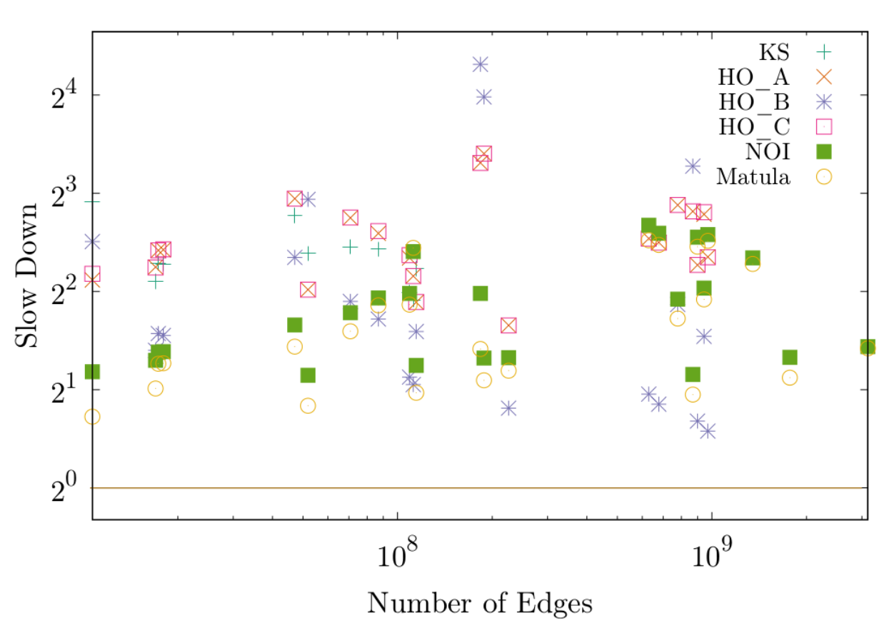
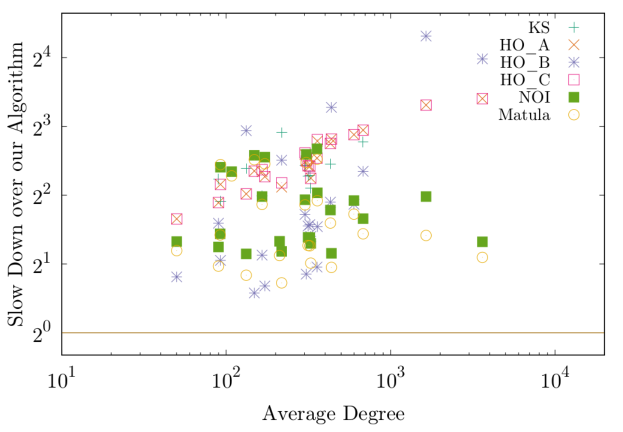
We also performed experiments on random hyperbolic graphs with and an average degree of . We generated graphs for each of the possible combinations of and average degree yielding a total of RHG graphs. Note that these graphs are hard instances for the inexact algorithms, as they contain few – usually only one – small cuts and both sides of the cut are large. From a total of runs, seqVieCut does not return the correct minimum cut in of runs and Matula does not return the correct minimum cut in of runs. KS, which crashes on large instances, returns non-optimal cuts in of the runs where it ran to completion.
Figure 4 shows the results for these experiments. On nearly all of these graphs, NOI is faster than HO. On sparse graphs with an average degree of , seqVieCut, Matula and NOI nearly have equal running time. On denser graphs with an average degree of , seqVieCut is faster than Matula and to times faster than NOI. HO_A and HO_C use preprocessing with the Padberg-Rinaldi heuristics. Multiple iterations of this preprocessing contract the RHG graph into two nodes. The running time of those algorithms is higher on sparse graphs and times higher on dense graphs compared to seqVieCut. Figure 5 shows a time breakdown for seqVieCut on large RHG graphs with . Around of the running time is in the label propagation step and the rest is mostly spent in graph contraction. The correcting step has low running time on most graphs, as it is not performed on large clusters.
Real-World Graphs
The third set of graphs we use in our experiments are -cores of large real-world social and web graphs. On these graphs, no non-optimal minimum cuts were returned by any algorithm except for KS, which gave non-optimal results. However, as most of these graph instances have multiple minimum cuts, even exact algorithms usually output different cuts on multiple runs. Figure 6 gives slowdown plots to the fastest algorithm (seqVieCut in each case) for the real-world graphs. On these graphs, seqVieCut is the fastest algorithm, far faster than the other algorithms. Matula is not much faster than NOI, as most of the running time is in the first iteration of their CAPFOREST algorithm, which is similar for both algorithms. On the largest real-world graphs, seqVieCut is approximately times faster than the next fastest algorithm Matula. We also see that seqVieCut, Matula and NOI all perform better on denser graphs. For Matula and NOI, this can most likely be explained by the smaller vertex priority queue. For seqVieCut, this is mainly due to better cache locality. As HO does not benefit from denser graphs, it has high slow down on dense graphs.
The highest speedup in our experiments is in the -core of gsh-2015-host, where seqVieCut is faster than the next fastest algorithm (Matula) by a factor of . The lowest speedup is in the -core of twitter-2010, where seqVieCut is faster than the next fastest algorithm (HO_B). The average speedup factor of seqVieCut to the next fastest algorithm is . NOI and Matula perform badly on the cores of the graph twitter-2010. This graph has a very low diameter (average distance on the original graph is ), and as a consequence the priority queue used in these algorithms is filled far quicker than in graphs with higher diameter. Therefore the priority queue operations become slow and the total running time is very high.


To summarize, both in generated and real-world graphs, even in sequential runs seqVieCut is up to a factor of faster than the state of the art, while achieving a high solution quality even for hard instances such as the hyperbolic graphs. The performance of seqVieCut is especially good on the real-world graphs, presumably as these graphs have high locality.
Shared-Memory Parallelism
Figure 7 shows the speedup of parVieCut compared to the sequential variant and to the next fastest algorithm, which is Matula in all of the large graph examined. We examine the largest graphs from each of the three graph classes and perform parallel runs using threads. We also perform experiments with threads, as the machine has cores and supports multi-threading. The harmonic mean of the speedup of parVieCut on large graphs with threads is . ( threads: ) and all runs computed the exact minimum cut. Compared to the next fastest sequential algorithm Matula, this is an average harmonic speedup factor of ( threads: ). parVieCut scales especially well on the clustered Erdős-Rényi graphs, presumably as these dense graphs contain many high-degree vertices and have a rather low number of vertices. Figure 8 shows average running time breakdowns averaged over all graphs. For this figure, the correcting algorithm is turned off for the two Erdős-Rényi graphs. With one thread, label propagation uses of the total running time and with threads, of the total running time. Thus the different parts of the algorithm parallelize equally well.

6 Random Edge Contraction
We now evaluate the variant of our algorithm that uses random edge contractions similar to the algorithm of Karger and Stein before running VieCut on the contracted graph. The edge contractions promise faster results but increase the error rate of the algorithm. This section shows experiments which detail error rate, error severity and running times for the heuristic and approximation algorithms. We repeat the experiments of the previous section, but now with only inexact algorithms. In addition to (the one iteration-only version of) KS, Matula and VieCut, we add VieCut C50, VieCut C75, VieCut C90, which contract , and of all vertices before running VieCut.

Clustered Erdős-Rényi Graphs
Figure 10 shows the running time for the random edge contraction algorithm variants compared to VieCut on dense clustered Erdős-Rényi graphs. We can see that VieCut C75 and VieCut C90 are always faster than VieCut, with VieCut C90 being faster by a factor of to than VieCut and VieCut C75 being faster by a factor of to .
Figure 9 (left) shows the average distance to the optimal cut for all algorithms which do not guarantee optimality, both as the difference and the factor of the returned cut to the optimal. In these highly regular graphs, we find the optimal cut if none of the low-weight edges between the clusters is contracted. Otherwise we find a cut where one side is only a single vertex. On average, this cut is around twice the value of the minimum cut. The algorithms all have an average cut factor of up to on all graphs, depending on how many vertices we contract. KS has a similar error rate on the graphs where it finishes. Both VieCut and Matula have no errors on these graphs.
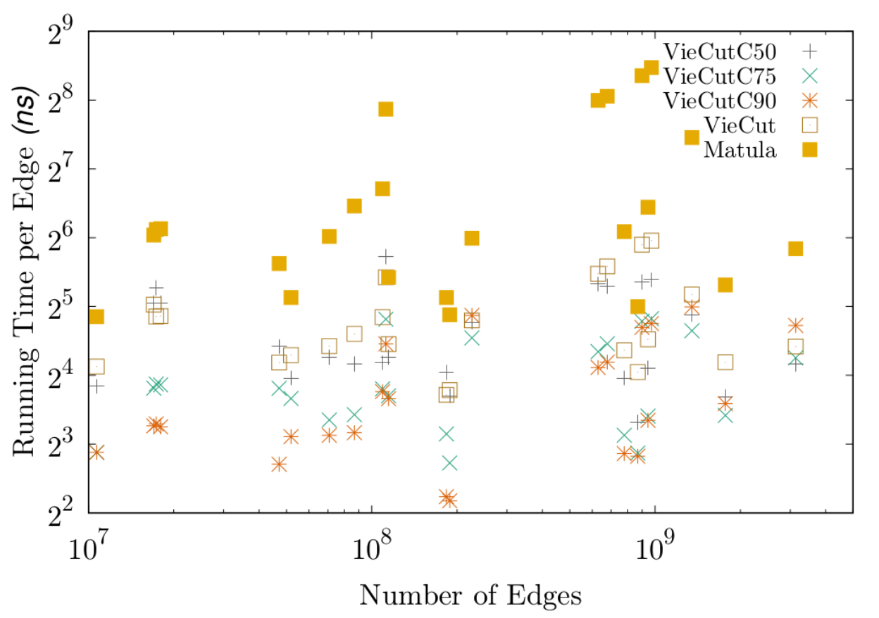
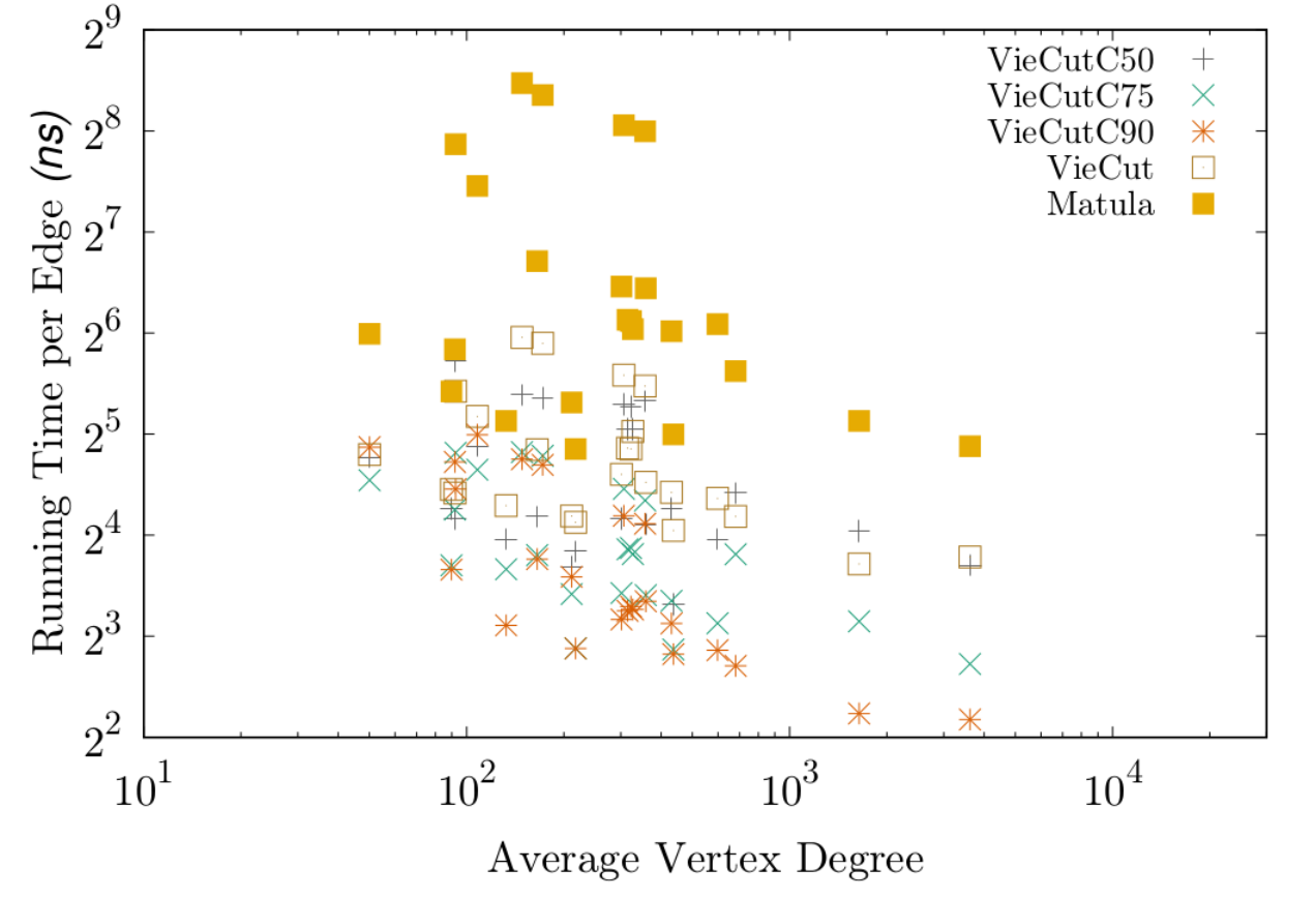
Real-World Graphs
Figure 11 shows the average running time for the random edge contraction variants of VieCut on real-world graphs. VieCut C90 is faster than VieCut by a factor of up to . The lowest speedup factor is (a slowdown of ). VieCut C75 has speedup factors between to compared to VieCut.
Figure 9 (middle) shows the average error rates. On these graphs, the average ratio of cut size to the optimal cut size is very low for the random contraction algorithms. The outlier for VieCut C75 and VieCut C90 is a single run of the graph twitter-2010 with , where one of the edges in the unique small cut (of value ) is contracted. The next smallest cut in the graph is a trivial cut with a cut value of , which is found. The algorithm finds optimal results in the other four iterations of this graph. On all other graphs, the cut factor is below . KS has an average cut rate of up to . VieCut and Matula have no errors on these graphs.

Random Hyperbolic Graphs
Figure 12 shows the running time of the algorithms on random hyperbolic graphs. VieCut C75 has a speedup of to compared to VieCut and VieCut C90 has a speedup of to .
Figure 9 (right) shows the error rate for RHG graphs. The error rate of VieCut is far lower than all other non-exact algorithms. Matula has a non-optimality factor that is between VieCut C50 and VieCut C75 but a smaller distance to the optimal solution than both of them. However, VieCut C75 is much faster than Matula, which is consistently slower than VieCut. Note that the 3 graphs in which Matula has a cut times as large as optimal are graphs with a minimum cut of , where Matula consistently returns cuts of value . Our implementation of Matula contracts all edges in the spanning forest with index .
Shared-Memory Parallelism

Figure 13 shows the speedup of the random contraction variants in comparison to VieCut. The RHG graph has a single smallest cut with value , followed by trivial cuts with a degree of each. VieCut and Matula return the correct minimum cut each run, VieCut C50 out of times, VieCut C75 times, VieCut C90 times and otherwise. Only VieCut C90 scales better than VieCut and has a speedup of up to compared to sequential VieCut. Due to the large number of clusters, where each cluster has many incident edges, the contraction step in VieCut C75 and VieCut C50 takes a long time.
The random contraction variants scale better in the large real-world graphs, where all algorithms return the minimum cut in all runs. On graph gsh-2015-host, VieCut C90 has a speedup of over , while VieCut C75 has a speedup of and VieCut has a speedup of with threads. On uk-2007-05, VieCut C90 has a speedup of over , VieCut C75 of over and VieCut a speedup of up to .
On the clustered Erdős-Rényi graphs, the random edge contraction creates one or few very large blocks of vertices. Again, VieCut and Matula always return the correct minimum cut. Out of runs on clustered Erdős-Rényi graphs, VieCut C50 returns the minimum cut in cases, VieCut C75 in cases and VieCut C90 in cases. On these very dense and unstructured graphs, random contraction has a high error rate and does not significantly speed up VieCut. VieCut however has a speedup of up to on these graphs. Figure 14 shows the average speedup of the algorithms compared to their performance with one thread on machine B.

In summary, the random contraction variants can improve the running time of VieCut even further, especially when we have many threads. However, the random contraction increases the error rate of the algorithm by a large margin and should therefore only be used if running time is more important than absolute solution quality.
5 Conclusion
We presented the linear-time heuristic algorithm VieCut for the minimum cut problem. VieCut is based on the label propagation algorithm [157] and the Padberg-Rinaldi heuristics [152]. Both for real-world graphs and a varied family of generated graphs, VieCut is significantly faster than the state of the art. The algorithm has far higher solution quality than other heuristic algorithms while also being faster. Additionally, we propose a variant of our algorithm to further speed up computations at the expense of higher error rates. Important future work includes checking whether using different clustering techniques affect the observed error probability. However, these clustering algorithms generally have higher running time.
Chapter 3 Exact Global Minimum Cut
In the previous chapter, we introduced a heuristic shared-memory parallel algorithm for the global minimum cut problem called VieCut. In this chapter, we combine techniques from that algorithm, the algorithm of Padberg and Rinaldi [152] and the algorithm of Nagamochi, Ono and Ibaraki [143, 147], as introduced in Section 4, to engineer an exact shared-memory parallel algorithm for the minimum cut problem. Our algorithm achieves improvements in running time over existing exact algorithms by a multitude of techniques. First, we use our fast and parallel inexact minimum cut algorithm VieCut to obtain a better bound for the problem. Afterwards, we use reductions that depend on this bound to reduce the size of the graph much faster than previously possible. We use improved data structures to further lower the running time of our algorithm. Additionally, we parallelize the contraction routines of Nagamochi et al.[143, 147]. Overall, we arrive at a system that outperforms the state-of-the-art by a factor of up to sequentially, and when run in shared-memory parallel, by a factor of up to using cores.
The content of this chapter is based on [90].
In the following sections we detail our exact shared-memory parallel algorithm for the minimum cut problem that is based on the algorithms of Nagamochi et al., as described in Section 1 and the VieCut algorithm described in Chapter 2 of this thesis. We aim to modify the algorithm of Nagamochi et al.in order to find exact minimum cuts faster and in parallel.
We start this chapter with optimizations to the sequential algorithm of Nagamochi et al. First we show how to save work by first performing the inexact VieCut algorithm to lower the minimum cut upper bound . As shown in Chapter 2, VieCut often already finds a cut of value . We then give different implementations of the priority queue and detail the effects of the choice of queue on the algorithm. We show that the algorithm remains correct, even if we limit the priorities in the queue to , meaning that elements in the queue having a key larger than that will not be updated. This significantly lowers the number of priority queue operations necessary. Then we adapt the algorithm so that we are able to detect contractible edges in parallel efficiently. In Section 3, we put everything together and present a full system description. We then give experimental setup and results of our work in Section 4 before we briefly conclude this chapter in Section 5.
1 Sequential Optimizations
1 Lowering the Upper Bound
The upper bound for the minimum cut is an important parameter for contraction based minimum cut algorithms. For example, the algorithm of Nagamochi et al.[147] computes a lower bound for the connectivity of the two incident vertices of each edge and contracts all edges whose incident vertices have a connectivity of at least . Thus, it is possible to contract more edges if we manage to lower beforehand.
A trivial upper bound for the minimum cut is the minimum vertex degree, as it represents the trivial cut which separates the minimum degree vertex from all other vertices. We run VieCut to lower in order to allow us to find more edges to contract. Although VieCut is an inexact algorithm, in most cases it already finds the minimum cut [94] of the graph. As there are by definition no cuts smaller than the minimum cut, the result of VieCut is guaranteed to be at least as large as the minimum cut . We set to the result of VieCut when running the CAPFOREST routine and can therefore guarantee a correct result.
2 Bounded Priority Queues
Whenever we visit a vertex in the CAPFOREST algorithm, we update the priority of all of its neighbors in by adding the respective edge weight. Thus we perform a total of priority queue increase-weight operations in one call of the CAPFOREST algorithm. In practice, many vertices reach priority values much higher than and perform many priority increases until they reach their final value. We limit the values in the priority queue by , i.e. we do not update priorities that are already . Lemma 1.1 shows that this does not affect correctness of the algorithm.
Let be the value assigned to in the modified algorithm on graph and let be the -value of a node in the modified algorithm on .
1.1.
Limiting the values in the priority queue used in the CAPFOREST routine to a maximum of does not interfere with the correctness of the algorithm. For every edge with , it holds that . Therefore the edge can be contracted.
Proof.
As we limit the priority queue to a maximum value of , we cannot guarantee that we always pop the element with highest value if there are multiple elements that have values in . However, we know that the vertex that is popped from is either maximal or has .
We prove Lemma 1.1 by creating a graph by lowering edge weights (possibly to , effectively removing the edge) while running the algorithm, so that CAPFOREST on visits vertices in the same order (assuming equal tie breaking) and assigns the same values as the modified algorithm on .
We first describe the construction of . We initialize the weight of all edges in graph with the weight of the respective edge in and run CAPFOREST on . Whenever we check an edge and update a value , we check whether we would set . If this is the case, i.e. when , we set in to , which is lower by exactly the value by which is larger than , and non-negative. Thus, . As we scan every edge exactly once in a run of CAPFOREST, the weights of edges already scanned remain constant afterwards. This completes the construction of
Note that during the construction of edge weights were only decreased and never increased. Thus it holds that for any pair of nodes . If we ran the unmodified CAPFOREST algorithm on each edge would be assigned a value with . Thus for every edge it holds that .
Below we will show that for all edges . It then follows that for all edges it holds that . This implies that if then , which is what we needed to show.
It remains to show that for all edges . To show this claim we will show the following stronger claim. For any with after the th and before the th scan of an edge the modified algorithm on and the original algorithm on with the same tie breaking have visited all nodes and scanned all edges up to now in the same order and for all edges it holds that (we assume that before scanning an edge , ) and for all nodes it holds that . We show this claim by the induction on .
For observe that before the first edge scan for all edges and the same node is picked as first node due to identical tie breaking and the fact that at that point. Now for assume that the claim holds for and consider the scan of the edge. If for the edge scan a new node needs to be chosen from the priority queue by one of the algorithms then note that both algorithms will have to choose a node and they pick the same node as for all nodes . Then both algorithms scan the same incident edge of as in both algorithms the set of unscanned neighbors of is identical. If neither algorithm has to pick a new node then both have scanned the same edges of the same current node and due to identical tie breaking will pick the same next edge to scan. Let this edge be . By induction at this time. As is unscanned which implies that . If then the modified algorithm on and the original algorithm on will set the value of to the same value, namely . If , then is set to and is set to , which leads to being set to . Thus and by induction for all . Additionally the modified algorithm on sets and the original algorithm on sets . It follows that and, thus, by induction for all . This completes the proof of the claim. ∎
Lemma 1.1 allows us to considerably lower the number of priority queue operations, as we do not need to update priorities that are bigger than . This optimization has even more benefit in combination with running VieCut to lower the upper bound , as we further lower the number of priority queue operations.
3 Priority Queue Implementations
Nagamochi et al.[147] use an addressable priority queue in their algorithm to find contractible edges. In this section we now address variants for the implementation of the priority queue. As the algorithm often has many elements with maximum priority in practice, the implementation of this priority queue can have major impact on the order of vertex visits and thus also on the edges that will be marked contractible.
Bucket Priority Queue
As our algorithm limits the values in the priority queue to a maximum of , we observe integer priorities in the range of . Hence, we can use a bucket queue that is implemented as an array with buckets. In addition, the data structure keeps the id of the highest non-empty bucket, also known as the top bucket, and stores the position of each vertex in the priority queue. Priority updates can be implemented by deleting an element from its bucket and pushing it to the bucket with the updated priority. This allows constant time access for all operations except for deletions of the maximum priority element, which have to check all buckets between the prior top bucket and the new top bucket, possibly up to checks. We give two possible implementations to implement the buckets so that they can store all elements with a given priority.
The first implementation, BStack uses a dynamic array (std::vector) as the container for all elements in a bucket. When we add a new element to the array, we push it to the back of the array. .pop_max() returns the last element of the top bucket. Thus, our algorithm will always visit the element next whose priority was just increased. It thus does not fully explore all vertices in a region and instead behaves more similar to a depth-first search.
The other implementation, BQueue uses a double ended queue (std::deque) as the container instead. A new element is pushed to the back of the queue and .pop_max() returns the first element of the top bucket. This results in a variant of our algorithm, which behaves more similar to a breadth-first search in that it first explores the vertices that have been discovered earlier, i.e. are closer to the source vertex in the graph.
Bottom-Up Binary Heap
A binary heap [193] is a binary tree (implemented as an array, where element has its children in index and ) which fulfills the heap property, i.e. each element has priority that is not lower than either of its children. Thus the element with highest priority is the root of the tree. The tree can be made addressable by using an array of indices, in which we save the position of each vertex. We use a binary heap using the bottom-up heuristics [192], in which we sift down holes that were created by the deletion of the top priority vertex. Priority changes are implemented by sifting the addressed element up or down in the tree. Operations have a running time of up to to sift an element up or down to fix the heap property.
In .pop_max(), the Heap priority queue does not favor either old or new elements in the priority queue and therefore this implementation can be seen as a middle ground between the two bucket priority queues.
2 Parallel CAPFOREST
We modify the algorithm in order to quickly find contractible edges using shared-memory parallelism. The pseudocode can be found in Algorithm 2. The proofs in this section show that the modifications do not violate the correctness of the algorithm. Detailed proofs for the original CAPFOREST algorithm and the modifications of Nagamochi et al.for weighted graphs can be found in [147].
The idea of the our algorithm is as follows: We aim to find contractible edges using shared-memory parallelism. Every processor selects a random vertex and runs Algorithm 2, which is a modified version of CAPFOREST [143, 147] where the priority values are limited to , the current upper bound of the size of the minimum cut. We want to find contractible edges without requiring that every process looks at the whole graph. To achieve this, every vertex will only be visited by one process. Compared to limiting the number of vertices each process visits this has the advantage that we also scan the vertices in sparse regions of the graph which might otherwise not be scanned by any process.
Figure 1 shows an example run of Algorithm 2 with . Every process randomly chooses a start vertex and performs Algorithm 2 on it to “grow a region” of scanned vertices. As we want to employ shared-memory parallelism to speed up the algorithm, we share an array between all processes to denote whether a vertex has already been visited. If a vertex has already been visited by a process, it will not be visited by any other processes. Additionally, every process keeps a local blacklist for vertices that the process attempted to visit but that were already visited by another process before and were thus ignored by this process. Note that is not shared between processes. We need this blacklist to ensure correctness, as a process may only contract edges that are not adjacent to a vertex previously blacklisted by that process (proof in Lemma 2.2). For every vertex we keep a value , which denotes the total weight of edges connecting to already scanned vertices. Over the course of a run of the algorithm, every edge is given a value (equal to right after scanning ) which is a lower bound for the smallest cut . We mark an edge as contractible (more accurately, we union the incident vertices in the shared concurrent union-find data structure [12]), if . Note that this does not modify the graph, it just remembers which nodes to collapse. The actual node collapsing happens in a postprocessing step. Nagamochi and Ibaraki showed [147] that contracting only the edges that fulfill the condition in line is equivalent.
As the set of disconnected edges is different depending on the start vertex, we looked into visiting every vertex by a number of processes up to a given parameter to find more contractible edges. However, this did generally result in higher total running times and thus we only visit every vertex once.
After all processes are finished, every vertex was visited exactly once (or possibly zero times, if the graph is disconnected). On average, every process has visited roughly vertices and all processes finish at the same time. We do not perform any form of locking of the elements of , as this would come with a running time penalty for every write and the only possible race condition with concurrent writes is that a vertex is visited more often, which does not affect correctness of the algorithm.
However, as we terminate early and no process visits every vertex, we cannot guarantee that the algorithm actually finds a contractible edge. However, in practice, this only happens if the graph is already very small ( vertices in all of our experiments). We can then run the (sequential) CAPFOREST routine to find at least one edge which can be contracted. In line and of Algorithm 2 we compute the value of the cut between the scanned and unscanned vertices and update if this cut is smaller than it. This optimization to the CAPFOREST algorithm was first given by Nagamochi et al.[147].
In practice, many vertices reach values of that are much higher than and therefore need to update their priority in often. As previously detailed, we limit the values in the priority queue by and do not update priorities that are already greater or equal to . This allows us to considerably lower the number of priority queue operations per vertex.
2.1.
Algorithm 2 is correct.
As Algorithm 2 is a modified variant of CAPFOREST [143, 147], we use the correctness of their algorithm and show that our modifications cannot result in incorrect results. In order to show this we need the following lemmas:
2.2.
The following modifications to the CAPFOREST algorithms do not result in incorrect results.
- 1.
Multiple instances of Algorithm 2 can be run in parallel with all instances sharing a parallel union-find data structure.
- 2.
Early termination does not affect correctness
- 3.
For every edge , where neither nor are blacklisted, is a lower bound for the connectivity , even if the set of blacklisted vertices is not empty.
- 4.
When limiting the priority of a vertex in to , it still holds that the vertices incident to an edge with have connectivity .
Proof.
A run of the CAPFOREST algorithm finds a non-empty set of edges that can be contracted without contracting a cut with value less than [143]. We show that none of our modifications can result in incorrect results:
- 1.
The CAPFOREST routine can be started from an arbitrary vertex and finds a set of edges that can be contracted without affecting the minimum cut . This is true for any vertex . As we do not change the underlying graph but just mark contractible edges, the correctness is obviously upheld when running the algorithm multiple times starting at different vertices. This is also true when running the different iterations in parallel, as long as the underlying graph is not changed.
Marking the edge as contractible is equivalent to performing a Union of vertices and . The Union operation in a union-find data structure is commutative and therefore the order of unions is irrelevant for the final result. Thus performing the iterations successively has the same result as performing them in parallel.
- 2.
Over the course of the algorithm we set a value for each edge and we maintain a value that never increases. We contract edges that have value at the time when is set. For every edge, this value is set exactly once. If we terminate the algorithm prior to setting for all edges, the set of contracted edges is a subset of the set of edges that would be contracted in a full run and all contracted edges fulfill at termination. Thus, no edge contraction contracts a cut that is smaller than .
- 3.
Let be an edge and let be the set of nodes blacklisted at the time when is scanned. We show that for an edge , , where with vertices and edges and is the graph with all blacklisted vertices and their incident edges removed. As the removal of vertices and edges can not increase edge connectivities and is contractible.
Whenever we visit a vertex , we decide whether we blacklist the vertex. If we blacklist the vertex , we immediately leave the vertex and do not change any values or for any other vertex or edge. As vertex is marked as blacklisted, we will not visit the vertex again and the edges incident to only affect .
As edges incident to any of the vertices in do not affect , the value of in the algorithm with the blacklisted in is equal to the value of in , which does not contain the blacklisted vertices in and their incident edges. On this is equivalent to a run of CAPFOREST without blacklisted vertices and due to the correctness of CAPFOREST [147] we know that for every edge .
Note that in we only exclude the vertices that are in . It is possible that a node that was unvisited when was scanned might get blacklisted later, however, this does not affect the value of as the value is set when an edge is scanned and never modified afterwards.
- 4.
Proof in Lemma 1.1.
We can combine the sub-proofs (3) and (4) by creating the graph , in which we remove all edges incident to blacklisted vertices and decrease edge weights to make sure no is strictly larger than . As we only lowered edge weights and removed edges, for every edge between two not blacklisted vertices , or and thus we only contract contractible edges. As none of our modifications can result in the contraction of edges that should not be contracted, Algorithm 2 is correct. ∎
3 Putting Things Together
Algorithm 3 shows the overall structure of the algorithm. We first run VieCut to find a good upper bound for the minimum cut. Afterwards, we run Algorithm 2 to find contractible edges. In the unlikely case that none were found, we run CAPFOREST [147] sequentially to find at least one contractible edge. We create a new contracted graph using parallel graph contraction with the hash-based shared-memory parallel contraction technique outlined in the previous chapter. This process is repeated until the graph has only two vertices left. Whenever we encounter a collapsed vertex with a degree of lower than , we update the upper bound. We return the smallest cut we encounter in this process.
If we also want to output the minimum cut, for each collapsed vertex in we store which vertices of are included in . When we update , we store which vertices are contained in the minimum cut. This allows us to see which vertices are on one side of the cut.
4 Experiments and Results
1 Experimental Setup and Methodology
We implemented the algorithms using C++-17 and compiled all codes using g++-7.1.0 with full optimization (-O3). Our experiments are conducted on a machine with two Intel Xeon E5-2643 v4 with 3.4GHz with 6 CPU cores each and hyper-threading enabled, and 1.5 TB RAM in total. We perform five repetitions per instance and report average running time.
Performance plots relate the fastest running time to the running time of each other algorithm on a per-instance basis. For each algorithm, these ratios are sorted in increasing order. The plots show the ratio on the y-axis. A point close to zero indicates that the running time of the algorithm was considerably worse than the fastest algorithm on the same instance. A value of one therefore indicates that the corresponding algorithm was one of the fastest algorithms to compute the solution. Thus an algorithm is considered to outperform another algorithm if its corresponding ratio values are above those of the other algorithm. In order to include instances that were too big for an algorithm, i.e. some implementations are limited to 32bit integers, we set the corresponding ratio below zero.
2 Algorithms
There have been multiple experimental studies that compare exact algorithms for the minimum cut problem [37, 94, 100]. All of these studies report that the algorithm of Nagamochi et al.and the algorithm of Hao and Orlin outperform other algorithms, such as the algorithms of Karger and Stein [105] or the algorithm of Stoer and Wagner [178], often by multiple orders of magnitude. Among others, we compare ourselfs against two available implementations of the sequential algorithm of Nagamochi et al.[143, 147]. We use our own implementation of the algorithm of Nagamochi et al.[143, 147], written in C++ (NOI-HNSS) which was implemented as part of VieCut (Chapter 2) and uses a binary heap. We use this algorithm with small optimizations in the priority queue as a base of our implementation. Chekuri et al.[37] give an implementation of the flow-based algorithm of Hao and Orlin using all optimizations given in the paper (variant ho in [37]), implemented in C, in our experiments denoted as HO-CGKLS. They also give an implementation of the algorithm of Nagamochi et al.[143, 147], denoted as NOI-CGKLS, which uses a heap as its priority queue data structure (variant ni-nopr in [37]). As their implementations use signed integers as edge ids, we include their algorithms only for graphs that have fewer than edges. Most of our discussions focus on comparisons to the NOI-HNSS implementation as this outperforms the implementations by Chekuri et al..
Gianinazzi et al.[75] give a MPI implementation of the algorithm of Karger and Stein [105]. We performed preliminary experiments on small graphs which can be solved by NOI-HNSS, NOI-CGKLS and HO-CGKLS in less than seconds. On these graphs, their implementation using processes took more than minutes, which matches other studies [37, 100, 94] that report bad real-world performance of (other implementations of) the algorithm of Karger and Stein. Gianinazzi et al.report a running time of seconds for RMAT graphs with and an average degree of , using cores. As NOI-HNSS can find the minimum cut on RMAT graphs [113] of equal size in less than seconds using a single core, we do not include the implementation in [75] in our experiments.
As our algorithm solves the minimum cut problem exactly, we do not include the -approximation algorithm of Matula [136] and our inexact algorithm VieCut in the experiments.
3 Instances
We use a set of graph instances that was also used for experiments in Chapter 2. The set of instances contains -cores [18] of large undirected real-world graphs taken from the 10th DIMACS Implementation Challenge [15] as well as the Laboratory for Web Algorithmics [24, 25]. Additionally it contains large random hyperbolic graphs [119, 131] with and . A detailed description of the graph instances is given in Section 5 (Graph family A). These graphs are unweighted, however contracted graphs that are created in the course of the algorithm have edge weights.

4 Sequential Experiments
We limit the values in the priority queue to , in order to significantly lower the number of priority queue operations needed to run the contraction routine. In this experiment, we want to examine the effects of different priority queue implementations and limiting priority queue values have on sequential minimum cut computations. We also include variants which run VieCut first to lower .
We start with sequential experiments using the implementation of NOI-HNSS. We use two variants: NOI limits values in the priority queue to while NOI-HNSS allows arbitrarily large values in . For NOI, we test the three priority queue implementations, BQueue, Heap and BStack. As the priority queue for NOI-HNSS has priorities of up to the maximum degree of the graph and the contracted graphs can have very large degrees, the bucket priority queues are not suitable for NOI-HNSS. Therefore we only use the implementation of NOI-HNSS [94].
The variants NOI-HNSS-VieCut and NOI-Heap-VieCut first run the shared-memory parallel algorithm VieCut using all threads to lower before running the respective sequential algorithm. We report the total running time, e.g. the sum of VieCut and NOI.


Priority Queue Implementations
Figure 2 shows the results for hyperbolic graphs and Figure 3 shows the results for real-world graphs, normalized by the running time of NOI-Heap-VieCut. Figure 4 gives performance plots for all graphs from both graph families. We can see that in nearly all sequential runs, NOI-BStack is faster than NOI-BQueue. This can be explained as this priority queue uses std::vector instead of std::deque as its underlying data structure and thus has lower access times to add and remove elements. As all vertices are visited by the only thread, the scan order does not greatly influence how many edges are contracted.
In the random hyperbolic graphs, nearly no vertices in NOI-HNSS reach priorities in that are much larger than . Usually, fewer than of edges do not incur an update in . Thus, NOI-HNSS and NOI-Heap have practically the same running time. NOI-BStack is usually slower.
As the real-world graphs are social network and web graphs, they contain vertices with very high degrees. In these vertices, NOI-HNSS often reaches priority values of much higher than and NOI can actually save priority queue operations. Thus, NOI-Heap is up to times faster than NOI-HNSS with an average (geometric) speedup factor of . Also, in contrast to the random hyperbolic graphs, NOI-BStack is faster than NOI-HNSS on real-world graphs. Due to the low diameter of web and social graphs, the number of vertices in is very large. This favors the BStack priority queue, as it has constant access times. The average geometric speedup of NOI-BStack compared to NOI-Heap is .
Reduction of by VieCut
In this experiment we aim to reduce by running VieCut before NOI. While the other algorithms are slower for denser random hyperbolic graphs, both algorithms NOI-HNSS-VieCut and NOI-Heap-VieCut are faster in these graphs with higher density. This happens as the variants without VieCut find fewer contractible edges and therefore need more rounds of CAPFOREST. The highest speedup compared to NOI-Heap is reached in random hyperbolic graphs with and an average density of , where NOI-Heap-VieCut has a speedup of factor .
NOI-Heap-VieCut is fastest on most real-world graphs, however when the minimum degree is very close to the minimum cut , running VieCut can not significantly lower . Thus, the extra work to run VieCut takes longer than the time saved by lowering the upper bound . The average geometric speedup factor of NOI-Heap-VieCut on all graphs compared to the variant without VieCut is .
In the performance plots in Figure 4 we can see that NOI-Heap-VieCut is fastest or close to the fastest algorithm in all but the very sparse graphs, in which the algorithm of Nagamochi et al.[147] is already very fast [94] and therefore using VieCut cannot sufficiently lower and thus the running time of the algorithm. NOI-CGKLS and HO-CGKLS are outperformed on all graphs.

5 Shared-memory parallelism
Overlapping Scan Regions
We examine whether it is useful to overlap the regions scanned by each thread. For this purpose we introduce a parameter which indicates how many threads can scan each processor. A value of executes algorithm 2, any larger value replaces with a counter indicating how many threads already scanned vertex . If , no further threads may scan it.
Figure 5 shows results for ParCut-BQueue with processes for values of from to on a set of large graphs ( real-world graphs, RHG graphs). In general, lower values of have lower running times for Algorithm 2, however the amounts of contracted edges can be lower, especially when many vertices have degree not too much higher than , as those can only be contracted depending on the order of vertex scans. On out of the graphs, has the best performance, just in the graph rhg_25_8_1 with minimum degree and , and are slightly faster. Thus we set parameter to and do not use overlapping scan regions.

We run experiments on of the largest graphs in the data sets using up to threads on cores. First, we compare the performance of Algorithm 3 using different priority queues: ParCut-Heap, ParCut-BStack and ParCut-BQueue all limit the priorities to , the result of VieCut. In these experiments, VieCut takes up between of the total running time with an average of . Figure 6 shows how well the algorithms scale with increased number of processors. Figure 7 shows the speedup compared to the fastest sequential algorithm of Section 4. On all graphs, ParCut-BQueue has the highest speedup when using threads. On real-world graphs, ParCut-BQueue also has the lowest total running time. In the large random hyperbolic graphs, in which the priority queue is usually only filled with up to elements, the worse constants of the double-ended queue cause the variant to be slightly slower than ParCut-Heap also even when running with threads. In the two large real-world graphs that have a minimum degree of , the sequential algorithm NOI-BStack contracts most edges in a single run of CAPFOREST - due to the low minimum degree, the priority queue operations per vertex are also very low. Thus, ParCut using only a single thread has a significantly higher running time, as it runs VieCut first and performs graph contraction using a concurrent hash table, as described in Section 1, which is slower than sequential graph contraction when using just one thread. In graphs with higher minimum degree, NOI needs to perform multiple runs of CAPFOREST. By lowering using VieCut we can contract significantly more edges and achieve a speedup factor of up to compared to the fastest sequential algorithm NOI-Heap. On twitter-2010, , ParCut-BQueue has a speedup of to NOI-HNSS, to NOI-CGKLS and a speedup of to HO-CGKLS. The other graphs have more than edges and are thus too large for NOI-CGKLS and HO-CGKLS.
5 Conclusion
We presented a shared-memory parallel exact algorithm for the minimum cut problem. Our algorithm is based on the algorithms of Nagamochi et al.[143, 147] and our work described in Chapter 2. We use different data structures and optimizations to decrease the running time of the algorithm of Nagamochi et al.by a factor of up to . Using additional shared-memory parallelism we further increase the speedup factor to up to . Future work includes checking whether our sequential optimizations and parallel implementation can be applied to the -approximation algorithm of Matula [136].
Chapter 4 Finding All Minimum Cuts
We present a practically efficient algorithm that finds all global minimum cuts in huge undirected graphs. Our algorithm uses a multitude of kernelization rules to reduce the graph to a small equivalent instance and then finds all minimum cuts using an optimized version of the algorithm of Nagamochi, Nakao and Ibaraki [146]. Some of these techniques are adapted from techniques for the global minimum cut problem [152, 147] which we discussed in the previous chapters of this dissertation. Using these and newly developed reductions we are able to decrease the running time by up to multiple orders of magnitude compared to the algorithm of Nagamochi et al.[146] and are thus able to find all minimum cuts on graphs with up to billions of edges in a few minutes. Based on the cactus representation of all minimum cuts, we are able to find the most balanced minimum cut in time linear to the size of the cactus. As our techniques are able to find the most balanced minimum cut of graphs with billions of edges in minutes, this allows the use of minimum cuts as a subroutine in sophisticated data mining and graph analysis.
The content of this chapter is based on [92].
1 Algorithm Description
Our algorithm combines a variety of techniques and algorithms in order to find all minimum cuts in a graph. The algorithm is based on the contractions of edges which cannot be part of any minimum cut. Thus, we first show that an edge that is not part of any minimum cut in graph can be contracted. In contrast to the previous chapters, we now aim to maintain all minimum cuts.
1.1.
[105] If an edge is not part of any minimum cut in graph , all minimum cuts of remain in the resulting graph .
Proof.
Let be an arbitrary minimum cut of . For an edge , which is not part of any minimum cut, we know that , so either and are both in vertex set or both in vertex set . This is still the case in . Thus, the edge can be contracted even if we aim to find every minimum cut of . ∎
Lemma 1.1 is very useful to reduce the size of the graph with the usage of techniques to identify such edges. We now give a short overview of our algorithm and then explain the techniques in more detail. First, we use our shared-memory parallel heuristic minimum cut algorithm VieCut (as described in Chapter 2) in order to find an upper bound for the minimum cut which is likely to be the correct value. Having a tight bound for the minimum cut allows the contraction of many edges, as multiple reduction techniques depend on the value of the minimum cut. We adapt contraction techniques originally developed by Nagamochi et al.[143, 147] and Padberg et al.[151] (see Section 4) to the problem of finding all minimum cuts. Section 1 details these contraction routines. On the resulting graph we find all minimum cuts using an optimized variant of the algorithm of Nagamochi, Nakao and Ibaraki [146] and return the cactus graph which represents them all. A short description of the algorithm and an explanation of our engineering effort are given in Section 2. Afterwards, in Section 3 we show how we combine the parts into a fast algorithm to find all minimum cuts of large networks.
1 Edge Contraction
As shown in Lemma 1.1, edges that are not part of any minimum cut can be safely contracted. We build a set of techniques that aim to find contractible edges and run these in alternating order until neither of them finds any more contractible edges. We now give a short introduction to these.
For efficiency, we perform contractions in bulk. If our algorithm finds an edge that can be contracted, we merge the incident vertices in a thread-safe union-find data structure [12]. After each run of a contraction technique that finds contractible edges, we create the contracted graph using a shared-memory parallel hash table [134]. In this contracted graph, each set of vertices of the original graph is merged into a single node. The contraction of this vertex set is equivalent to contracting a spanning tree of the set. After contraction we check whether a vertex in the contracted graph has degree . If it does, we found a cut of smaller value and update to this value.
Connectivity-based Contraction
The connectivity of an edge is the weight of the minimum cut that separates and , i.e. the minimum s-t-cut. For an edge that has connectivity , we thus know that there is no cut separating and (i.e. no cut that contains ) that has value . Thus, we know that there cannot be a minimum cut that contains , as is by definition at least as large as . However, solving the minimum s-t-cut problem takes significant time, so computing the connectivity of each edge does not scale to large networks. Hence, as part of their algorithm for the global minimum cut problem, Nagamochi et al.[143, 147] give a subroutine that computes a lower bound for the connectivity of every edge of in a total running time of . Both the algorithm of Nagamochi et al.and the CAPFOREST subroutine that computes the connectivity lower bounds are outlined in Section 1. Each of the edges whose connectivity lower bound is already larger than can be contracted as it cannot be part of any minimum cut.
In Chapter 3 we give a fast shared-memory parallel variant of their algorithm. As that algorithm aims to find a single minimum cut, it also contracts edges that have connectivity equal to , as the only relevant cuts are ones better than the best cut known previously. As we want to find all minimum cuts, we can only contract edges whose connectivity is strictly larger than . Nagamochi et al.could prove that at least one edge has value in their routine and can thus be contracted. We do not have such a guarantee when trying to find edges that have connectivity . Consider for example an unweighted tree, whose minimum cut has a value of and each edge has connectivity as well.
Local Contraction Criteria
Padberg and Rinaldi [151] give a set of local reduction routines which determine whether an edge can be contracted without affecting the minimum cut. We describe these reductions in Section 2. Their reduction routines were shown to be very useful in order to find a minimum cut fast in practice [37, 100, 94] and are also used in our VieCut algorithm in Chapter 2. We adapt the routines originally developed for the minimum cut problem so that they hold for the problem of for finding all minimum cuts. Thus, we have to make sure that we do not contract cuts of value , as they might be minimal and additionally make sure that we do not contract edges incident to vertices that could have a trivial minimum cut, i.e. a minimum cut, where one side contains only a single vertex. Figure 1 shows examples and Lemma 1.2 gives a formal definition of these reduction rules.
1.2.
For an edge , is not part of any minimum cut, if fulfills at least one of the following criteria. Thus, all minimum cuts of are still present in and can be contracted.
- 1.
HeavyEdge:
- 2.
ImbalancedVertex:
- •
and , or
- •
and
- •
- 3.
ImbalancedTriangle:
with- •
and , and
- •
and
- •
- 4.
HeavyNeighborhood:
Proof.
- 1.
If , every cut that contains has capacity . Thus it can not be a minimal cut.
- 2.
Without loss of generality let be the vertex in question. The condition means that is heavier than all other edges incident to combined. Thus, for any non-trivial cut that contains , we can find a lighter cut by replacing with all other incident edges to , i.e. moving to the other side of the cut. As this is not true for the trivial minimum cut , we cannot contract an edge incident to a vertex that has weight .
- 3.
This condition is similar to (2). Let there be a triangle in the graph in which it holds for both and that the two incident triangle edges are heavier than the sum of all other incident edges. Then, every cut that separates and can be improved by moving and into the same side. As the cut could have vertex on either side, both vertices need to fulfill this condition. To make sure that we do not contract any trivial minimum cut, we check that both and have weighted vertex degree and thus can not represent a trivial minimum cut.
- 4.
In this condition we check the whole shared neighborhood of vertices and . Every cut that separates and must contain and for each shared neighbor at least one of the edges connecting them to . Thus, we sum over the lighter edge connecting them to the shared neighbors and have a lower bound of the minimum cut that separates and . If this is heavier than , we know that no minimum cut separates and .
∎
The conditions HeavyEdge and ImbalancedVertex can both be checked for the whole graph in a single run in linear time. While we can check condition ImbalancedTriangle when summing up the lighter incident edges for condition HeavyNeighborhood, exhaustively checking all triangles incurs a strictly worse than linear runtime, as a graph can have up to triangles [166]. Thus, we only perform linear-time runs as developed by Chekuri et al.[37] by marking the neighborhood of and while we check the conditions and do not perform the test on marked vertices.
Vertices with One Neighbor
Over the run of the algorithm, we occasionally encounter vertices that have only a single neighbor. Let be this vertex with one neighbor and be the only incident edge. As we update to the minimum degree whenever we perform a bulk edge contraction, : for an edge whose weight is , condition HeavyEdge will contract it. For an edge whose weight is , the edge represents a trivial minimum cut iff . This is the only minimum cut that contains , as every non-trivial cut containing has higher weight. Thus, we can contract for now and remember that it was contracted. If is decreased, we can forget about these vertices as the cuts are not minimal. When we are finished, we can re-insert all contracted vertices that have a trivial minimum cut. We perform this reinsertion in a bottom-up fashion (i.e. in reverse order to how they were contracted), as the neighbor could be contracted in a later contraction.
2 Finding All Minimum Cuts
We apply the reductions in the previous section exhaustively until they are not able to find a significant number of edges to contract. On the remaining graph we aim to find the cactus representation of all minimum cuts. Our algorithm for this purpose is based on the algorithm of Nagamochi, Nakao and Ibaraki [146]. While there is a multitude of algorithms for the problem of finding all minimum cuts, to the best of our knowledge there are no implementations accessible to the public and there is no practical experimentation on finding all minimum cuts. We base our algorithm on the algorithm of Nagamochi, Nakao and Ibaraki [146], as their algorithm allows us to run the reduction routines previously detailed in between recursion steps.
We give a quick sketch of their algorithm, for further details we refer the reader to [146]. To find all minimum cuts in graph , the algorithm chooses an edge in and uses a maximum flow to find the minimum s-t-cut . If there is no minimum cut that separates and and thus can be contracted. If , the edge is part of at least one minimum cut. They show that the strongly connected components of the residual graph represent all minimum cuts that contain (and potentially some more). For each connected component , they build a graph , in which all other connected components are contracted into a single vertex. We recurse on these component subgraphs and afterwards combine the minimum cut cactus graphs of the recursive calls to a cactus representation for . The combination of the cactus graphs begins by building a cactus graph representing the set of strongly connected components, in which each is represented by a single vertex . Each cactus is then merged with by replacing with . Inside this algorithm we re-run the contraction routines of Section 1. As they incur some computational cost and the graph does not change too much over different recursion steps, we only run the contraction routines every recursion levels.
As the contraction routines in Section 1 usually mark a large amount of edges that can be contracted in bulk, we represent the graph in the compressed sparse row format [186]. This allows for fast and memory-efficient accesses to vertices and edges, however, we need to completely rebuild the graph in each bulk contraction and also keep vertex information about the whole graph hierarchy to be able to see which vertices in the original graph are encompassed in a vertex in a coarser vertex and to be able to re-introduce the cactus edges that were removed. While this is efficient for the bulk contractions performed in the previous section, in this section we often perform single-edge contractions or contract a small block of vertices. For fast running times these operations should not incur a complete rebuild of the graph data structure. We therefore use a mutable adjacency list data structure where each vertex is represented by a dynamic array of edges to neighboring vertices. Each edge stores its weight, target and the ID of its reverse edge (as we look at undirected graphs). This allows us to contract edges and small blocks in time corresponding to the sum of vertex degrees. For each vertex in the original graph, we store information which vertex currently encompasses it and every vertex keeps a list of currently encompassed vertices of the original graph. All vertex and edge information is updated during each edge contraction. The same graph data structure is also used for the multiterminal cut problem in Part 3 of this work.
Edge Selection
The recursive algorithm of Nagamochi, Nakao and Ibaraki [146] selects an arbitrary edge for the maximum flow problem in each recursion step. If this edge has connectivity equal to the minimum cut, we create a recursive subproblem for each connected component of the residual graph. In order to reduce the graph size - and thus the amount of work necessary - quickly, we aim to select edges in which the largest connected component of the residual graph is as small as possible. The edge selection strategy Heavy searches for the highest degree vertex and chooses the edge from to its highest degree neighbor. The strategy WeightedHeavy does the same, but uses the vertices whose weighted degree is highest. The idea is that an edge between high-degree vertices is most likely ’central’ to the graph and thus manages to separate sizable chunks from the graph. The edge selection strategy Central aims to find a central edge more directly: we aim to find two vertices and with a high distance and take the central edge in their shortest paths. We find those vertices by performing a breadth-first search from a random vertex , afterwards performing a breadth-first search from the vertex encountered last. We then take the central edge in the shortest path (as defined from the second breadth-first search) from the two vertices encountered last in the two breadth-first searches. The edge selection strategy Random picks a random edge.
Degree-two Reductions
Over the course of this recursive contraction-based algorithm, we often encounter vertices with just two neighbors. Let be the vertex in question, which is connected to by edge and to by edge . We look at four cases, each looking at whether the weight of being equal to the weight of and being equal to , both conditions that can be checked in constant time. In three out of four cases, we are able to contract an incident edge.
and : Without loss of generality let be the heavier edge. As , the trivial cut is not a minimum cut. As by definition no cut in is smaller than , . Thus, excluding the path through , they have a connectivity of and any cut containing has weight and can thus not be minimal. We therefore know that is not part of any minimum cuts and can be contracted according to Lemma 1.1.
and : Without loss of generality let be the heavier edge. Analogously to the previous case we can show that no nontrivial cut contains . In this case, where , the trivial cut is minimal and therefore should be represented in the cactus graph. For all other minimum cuts that contain , we know that and will be in the same block (as ). Thus, will be represented in the cactus as a leaf incident to . We contract calling the resulting vertex and store which vertices of the original graph are represented by . Then we recurse. On return from the recursion we check which cactus vertex now encompasses and add an edge from this vertex to a newly added vertex representing all vertices encompassed by .
and : in this case we are not able to contract any edges without further connectivity information.
and : as , the trivial cut is minimal. If there are other minimum cuts that contain either or (e.g. that separate and ), we know that by replacing with (or vice-versa) the cut remains minimal. Such a minimum cut exists iff . We contract and remember this decision. As is still in the graph (merged with ), we are able to find each cut that separates and . If none exists, and and will be contracted later in the algorithm. When leaving the recursion, we can thus re-introduce vertex as a leaf connected to the vertex encompassing and . If and are in different vertices after leaving the recursion, there is at least one nontrivial cut that contains . We thus re-introduce as a cycle vertex connected to and , each with weight , and subtract from .
In three out of the four cases presented here, we are able to contract an edge incident to a degree-two vertex. We can check these conditions in total time for the whole graph. Over the course of the algorithm, we perform edge contractions and thus routinely encounter vertices whose neighborhood has been contracted and thus have a degree of two. Thus, these reductions are able to reduce the size of the graph significantly even if the initial graph is rather dense and does not have a lot of low degree vertices.
3 Putting it All Together
Algorithm 4 gives an overview over our algorithm to find all minimum cuts. Over the course of the algorithm we keep an upper bound for the minimum cut, initially set to the result of the inexact variant of the VieCut minimum cut algorithm [94] (Chapter 2). While the VieCut algorithm also offers an exact version [90] (Chapter 3), we use the inexact version, as it is considerably faster and gives a low upper bound for the minimum cut, usually equal to the minimum cut. As described in Section 1, we use this bound to contract degree-one vertices, high-connectivity edges and edges whose local neighborhood guarantees that they are not part of any minimum cut. We repeat this process until it is converged, as an edge contraction can cause other edges in the neighborhood to also become safely contractible. As this process often incurs a long tail of single edge contractions, we stop if the number of vertices was decreased by less than over a run of all contraction routines.
We then use the minimum cut algorithm of Nagamochi, Ono and Ibaraki [143, 147] on the remaining graph, as the following steps need the correct minimum cut. To find all minimum cuts in the contracted graph, we call our optimized version of the algorithm of Nagamochi et al.[146], as sketched in Section 2, and afterwards re-insert all minimum cut edges that were previously deleted. Before each recursive call of the algorithm of Nagamochi et al.[146], we contract edges incident to degree-one and eligible degree-two vertices. Every recursion levels we additionally check for connectivity-based edge contractions and local contractions.
4 Shared-Memory Parallelism
Algorithm 4 employs shared-memory parallelism in every step. When we run the algorithm in parallel, we use the parallel variant of VieCut [94]. Local contraction and marking of degree one vertices are parallelized using OpenMP [42]. For the first round of connectivity-based contraction, we use the parallel connectivity certificate used in the shared-memory parallel minimum cut algorithm detailed in Chapter 3 [90]. This connectivity certificate is essentially a parallel version of the connectivity certificate of Nagamochi et al.[143, 147], in which the processors divide the work of computing the connectivity bounds for all edges of the graph. In subsequent iterations every processor runs an independent run of the connectivity certificate of Nagamochi et al.on the whole graph starting from different random vertices in the graph. As the connectivity bounds given by the algorithm heavily depend on the starting vertex, this allows us to find significantly more contractible edges per round than running the connectivity certificate only once.
We use our exact shared-memory parallel minimum cut algorithm to find the exact minimum cut of the graph. The algorithm of Nagamochi et al.[146] is not shared-memory parallel, however we usually manage to contract the graph to a size proportional to the minimum cut cactus before calling them. Unfortunately it is not beneficial to perform the recursive calls embarrassingly parallel, as in almost all cases one of the connected components of the residual graph contains the vast majority of vertices and thus also has the overwhelming majority of work.
2 Applications
We can use the minimum cut cactus to find a minimum cut fulfilling certain balance criteria, such as a most balanced minimum cut, e.g. a minimum cut that maximizes min. Note that this is not equal to the most balanced --cut problem, which is NP hard [26]. Following that we show how to modify the algorithm to find the optimal minimum cut for other optimization functions.
One can find a most balanced minimum cut trivially in time , as one can enumerate all minimum cuts [104] and add up the number of vertices of the original graph on either side. We now show how to find a most balanced minimum cut of a graph in time, given the minimum cut cactus graph .
For every cut , we define the balance (or of the cut as the number of vertices of the original graph encompassed in the lighter side of the cut. Recall that for any node , is the number of vertices of represented by . For a leaf , we set its weight and set the balance to be the minimum of and . We root in an arbitrary vertex and depending on that root define as the sum of vertex weights in the subcactus rooted in ; and accordingly. For a cycle , we define with analogously as the balance of the minimum cut splitting the cycle so that the sub-cacti rooted in are on one side of the cut and the rest are on the other side (see blue line in Figure 2 for an example).
Let be the tree representation of where each cycle in is contracted into a single vertex. We perform a depth-first search on rooted on an arbitrary vertex and check the balance of every cut in when backtracking.
As is not necessarily a tree, we might encounter cycles and we explain next how to extend the depth first search to handle such cycles. Let be a cycle and be the vertex encountered first by the DFS. Due to the cactus graph structure of , the depth-first search backtracks from a vertex in that represents only after all subtrees rooted in are explored. Thus, we know the weight of all subtrees rooted in vertices when backtracking. The weight of is equal to minus the sum of these sub-cactus weights.
Examining all cuts in the cycle would take time, but as we only want to find the most balanced cut, we can check only a subset of them, as shown in Algorithm 5. and are queues, thus elements are ordered and the following operations are supported: queue adds an element to the back of the queue, called the tail of the queue, dequeue removes the element at the front of the queue, called the head of the queue. We implicitly use the fact that queues can only be appended to, thus an element was added to the queue after all elements that are closer to the head of the queue and before all elements that are closer to its tail.
The weight of a queue is denoted as the weight of its contents. For queue with , we use the notation to denote the weight of and as the weight of the queue that contains all cycle vertices not in .
In every step of the algorithm, the cut represented by the current state of the queues consists of the two edges connecting the queue heads to the tails of the respective other queue. Initially is empty and contains all elements, in order from to . In every step of the algorithm, we dequeue one element and queue it in the other queue. Thus, at every step each cycle vertex is in exactly one queue. When we check the balance of a cut, we compute the weight of each queue at the current point in time; and update , the best balance found so far, if is more balanced. As we only move one cycle vertex in each step, we can check the balance of an adjacent cut in constant time by adding and subtracting the weight of the moved vertex to the weights of each set.
2.1.
Algorithm 5 terminates after steps.
Proof.
In each step of Algorithm 5, one queue head is moved to the other queue. The algorithm terminates when is the head of for the second time. In the first step, is moved to , as the empty queue is the lighter one. The algorithm terminates after then performs a full round through both queues and is the head of again. At termination, was thus moved a total of three times, twice from to and once the other way. As no element can ’overtake’ in the queues, every vertex will be moved at most three times. Thus, we enter the loop at most times, each time only using a constant amount of time. ∎
In Algorithm 5, we only check the balance of a subset of cuts represented by edges in the cycle . Lemma 2.3 shows that none of the disregarded cuts can have balance better than and we thus find the most balanced minimum cut. We call a cut disregarded if its balance was never checked (Line ), and considered otherwise. In order to prove correctness of Algorithm 5, we first show the following Lemma:
2.2.
Each vertex in the cycle is dequeued from at least once in the algorithm.
Proof.
The algorithm terminates when is the head of for the second time. For this, it needs to be moved from to twice. As we queue elements to the back of a queue, all vertices are dequeued from before is dequeued from it for the second time. In order for to become the head of again, all elements that were added beforehand need to be dequeued from . ∎
2.3.
Algorithm 5 finds the most balanced minimum cut represented by cycle .
Proof.
We now prove for each that all disregarded cuts containing the cycle edge separating from are not more balanced than the most balanced cut found so far. As no disregarded cut can be more balanced than the most balanced cut considered in the algorithm, the output of the algorithm is the most balanced minimum cut; or one of them if multiple cuts of equal balance exist.
.
Let be the time that becomes the head of for the first time. Figure 3 shows the state of at that point in time. Let be the tail of at time for some integer . Right before , was head of the heavier queue and thus dequeued, i.e. has weight and is now head of .
From this point the algorithm considers cuts that separate from . While is not heavier than , we add more elements to the tail of (and check the respective cuts) until is the heavier queue. Let be the time when this happens and with be the tail of at this point. Note that at time , is about to be dequeued from . The red cut in Figure 3 shows the cut at time , where .
We now prove that all cuts in which is the head of and its tail is not between and cannot be more balanced than the most balanced cut considered so far.
For all cuts where is head of and also contains , is heavier than , as it contains all elements in plus at least one more. As , i.e. is already heavier when is its tail, all of these cuts are less balanced than .
For the cuts in which is in , i.e. is lighter than at time , we need to distinguish two cases, depending on whether is larger than or not.
If , all cuts in which is the head of and is in are less balanced than , as is lighter than it is at , where it was already not the heavier queue.
If , there might be cuts in which is the head of that are more balanced than in which is lighter than at time . Thus, consider time when was added to . Such a time must exist, since is initially empty. As is already the tail of at time , . At that time contained and potentially more vertices.
Still, , as otherwise would not have been added to . Obviously , as is even lighter when is dequeued. As is already not heavier than its complement, is more imbalanced than the cut examined just before time . Thus, all cuts where is the head of and is in are even more imbalanced, as is even lighter.
Coming back to the outline shown in Figure 3, we showed that for all cuts in which is head of and is lighter than at time (left of blue cut) and all cuts where is heavier than at time (below red cut) can be safely disregarded, as a more balanced cut than any of them was considered at some point between and . The algorithm considers next all cuts with as head of and the tail of between and . Thus, the algorithm will return a cut that is at least as balanced as the most balanced cut that separates and . This is true for every cycle vertex , which concludes the proof. ∎
This allows us to perform the depth-first search and find the most balanced minimum cut in in time . This algorithm can be adapted to find the minimum cut of any other optimization function of a cut that only depends on the (weight of the) edges on the cut and the (weight of the) vertices on either side of the cut. In order to retain the linear running time of the algorithm, the function needs to be evaluable in constant time on a neighboring cut. For example, we can find the minimum cut of lowest conductance. The conductance of a cut is defined as , where is the sum of degrees for all vertices in set . Note that this is not the minimum conductance cut problem, which is NP-hard [10], as we only look at the minimum cuts. To find the minimum cut of lowest conductance, we set the weight of a vertex to the sum of vertex degrees encompassed in . Otherwise the algorithm remains the same.
3 Experiments and Results
We now perform an experimental evaluation of the proposed algorithms. This is done in the following order: first analyze the impact of algorithmic components on our minimum cut algorithm in a non-parallel setting, i.e. we compare different variants for edge selection and see the impact of the various optimizations detailed in this work. Afterwards, we report parallel speedup on a variety of large graphs.
Experimental Setup and Methodology
We implemented the algorithms using C++-17 and compiled all code using g++ version 8.3.0 with full optimization (-O3). Our experiments are conducted on a machine with two Intel Xeon Gold 6130 processors with 2.1GHz with 16 CPU cores each and GB RAM in total. We perform five repetitions per instance and report average running time. In this section we first describe our experimental methodology. Afterwards, we evaluate different algorithmic choices in our algorithm and then we compare our algorithm to the state of the art. When we report a mean result we give the geometric mean as problems differ significantly in cut size and time.
Instances
We use a variety of graphs from the 10th DIMACS Implementation challenge [15] and the SuiteSparse Matrix Collection [46]. These are social graphs, web graphs, co-purchase matrices, cooperation networks and some generated instances. If a network has multiple connected components, we run on the largest. The list of graphs can be found in Section 5, where graph family (2A) shows a set of smaller instances and graph family (2B) shows a set of larger and harder to solve instances.
1 Edge Selection
Figure 4 shows the results for graph family (2A). We compute the cactus graph representing all minimum cuts using the edge selection variants Random, Central, Heavy and HeavyWeighted, as detailed in Section 2. As we want a majority of the running time in the algorithm of Nagamochi et al.[146], where we actually select edges, we run a variant of our algorithm that only contracts edges using connectivity-based contraction and then runs the algorithm of Nagamochi et al.[146].
We can see that in the graphs which cannot be contracted quickly, Random is significantly slower than all other variants. On cnr-2000, Random takes over seconds in average, whereas all other variants finish in approximately seconds. This happens independently of the random seed used, there is no large deviation in the running time on any of the graphs. On almost all graphs, the variants Heavy and HeavyWeighted are within of each other, which is not surprising, as the variants are almost identical. While it optimizes for ’edge centrality’ very directly, Central has two iterations of breadth-first search in each edge selection and thus a sizable overhead. For this reason it is usually slower than Heavy and is not the fastest algorithm on any graph. On graphs with large , all three variants manage to shrink the graph significantly faster than Random.
On graphs with a low value of , we can see that Random is slightly faster than the other variants. There is no significant difference in the shrinking of the graph, as almost all selected edges have connectivity larger than and thus only trigger a single edge contraction anyway. Thus, not spending the extra work of finding a ‘good’ edge results in a slightly lower running time. In the following we will use variant Heavy, which is the only variant that is never more than slower than the fastest variant on any graph.
2 Optimization
We now examine the effect of the different optimizations. For this purpose, we benchmarks different variants on a variety of graphs. We hereby compare the following variants that build on one another: as a baseline, BasicCactus runs the algorithm of Nagamochi, Nakao and Ibaraki [146] using Heavy edge selection on the input graph. +Connectivity additionally runs VieCut [94] to find an upper bound for the minimum cut and uses this to contract high-connectivity edges as described in Section 1. In addition to this, +LocalContract also contracts edges whose neighborhood guarantees that they are not part of any minimum cut, as described in Section 1 and Lemma 1.2. +DegreeOne runs also the last remaining contraction routine from Algorithm 4, contraction and re-insertion of degree-one vertices as described in Section 1. +C&LInCactus additionally runs high-connectivity and local contraction in every tenth recursion step. +D1InCactus additionally contracts and re-inserts degree-one vertices in every recursion step. FullAlgorithm also runs the degree-two contraction as described in Section 2. We compare these variants on the graph families (2A) and (2B) of Table 5. We use a timeout of minutes for each problem. If the baseline algorithm does not finish in the allotted time, we report speedup to the timeout, so a lower bound for the actual speedup.
Figure 5 shows the speedup of all variants to the baseline BasicCactus on all small graphs. We can see that already just adding +Connectivity gives a speedup of more than an order of magnitude for each of the graphs in the dataset. Most of the other optimizations manage to improve the running time of at least some instances by a large margin. Especially +DegreeOne, which is the first contraction for edges that are in a minimum cut, has speedups of multiple orders of magnitude in some instances. This is the case as minimum cut edges that are incident to a degree-one vertex previously incur a flow problem on the whole graph each. However, it is very easy to see that the edge will be part of exactly one minimum cut, thus we can contract and re-insert it in constant time. Especially in graphs whose minimum cut is , all edges can be quickly contracted, as they will either be incident to a degree-one vertex or be quickly certified to have a connectivity value of .
While rerunning Connectivity and LocalContract inside of the recursive algorithm of Nagamochi et al.[146] does usually not yield a large speedup, many graphs develop degree-one vertices by having their whole neighborhood contracted. Thus, +D1InCactus has a significant speedup for most graphs in which is sufficiently large. FullAlgorithm has an even larger speedup on these graphs, even when the minimum cut is significantly higher than , as there are often cascading effects where the contraction of an edge incident to a degree-two vertex often lowers the degree of neighboring vertices to two.
Figure 6 shows the speedup of all variants on large graphs. As BasicCactus is not able to solve any of these instances in minutes, we use +Connectivity as a baseline. The results are similar to Figure 5, but we can see even clearer how useful the contraction of degree-two vertices is in finding all minimum cuts: FullAlgorithm often has a speedup of more than an order of magnitude to all other variants and is the only variant that never times out.
| Name | max. | max. | seq. t | par. t | ||||
|---|---|---|---|---|---|---|---|---|
| friendster | M | B | M | 1 | 897 | 1 793 | s | s |
| twitter7 | M | B | M | 1 | 47 | 1 893 | s | s |
| uk-2007-05 | M | B | M | 1 | 49 984 | M | s | s |
3 Shared-memory Parallelism
Table 1 shows the average running times of our algorithm both sequential and with threads on huge social and web graphs. Each of these graphs has more than a billion of edges and more than a million vertices in the cactus graph depicting all minimum cuts. On these graphs we have a parallel speedup factor of x to x using threads. On all of these graphs, a large part of the running time is spent in the first iteration of the kernelization routines, which already manages to contract most dense blocks in the graph. Thus, all subsequent operations can be performed on significantly smaller problems and are therefore much faster.
4 Conclusion
We engineered an algorithm to find all minimum cuts in large undirected graphs. Our algorithm combines multiple kernelization routines with an engineered version of the algorithm of Nagamochi, Nakao and Ibaraki [146] to find all minimum cuts of the reduced graph. Our experiments show that our algorithm can find all minimum cuts of huge social networks with up to billions of edges and millions of minimum cuts in a few minutes on shared memory. We found that especially the contraction of high-connectivity edges and efficient handling of low-degree vertices can give huge speedups. Additionally we give a linear time algorithm to find the most balanced minimum cut given the cactus graph representation of all minimum cuts. Future work includes finding all near-minimum cuts.
Chapter 5 Dynamic Minimum Cut
In this chapter, we give the first implementation of a fully-dynamic algorithm for the minimum cut problem in a weighted graph. Our algorithm maintains an exact global minimum cut under edge insertions and deletions. For edge insertions, we use the approach of Henzinger [96] and Goranci et al.[79], who maintain a compact data structure of all minimum cuts in a graph and invalidate only the minimum cuts that are affected by an edge insertion. We use the algorithm presented in Chapter 4 to compute all minimum cuts in a graph. For edge deletions, we use the push-relabel algorithm of Goldberg and Tarjan [77] to certify whether the previous minimum cut is still a minimum cut. As we only need to certify whether an edge deletion changes the value of the minimum cut, we can perform optimizations that significantly improve the speed of the push-relabel algorithm for our application. In particular, we develop a fast initial labeling scheme and terminate early when the connecitivity value is certified.
An important observation for dynamic minimum cut algorithms is that graphs often have a large set of global minimum cuts. We can see this in the experimental section of Chapter 4, where we aim to find all minimum cuts in huge graphs. Thus, dynamic minimum cut algorithms can avoid costly recomputation by storing a compact data structure representing all minimum cuts [96, 79] and only invalidate changed cuts in edge insertion. The data structure we use is a cactus graph, i.e. a graph in which every vertex is part of at most one cycle. A minimum cut in the cactus graph is represented by either a tree edge or two edges of the same cycle. For a graph with multiple connected components, i.e. a graph whose minimum cut value , the cactus graph has an empty edge set and one vertex corresponding to each connected component.
The content of this chapter is based on [89].
The rest of this chapter is organized as follows. We start by explaining the incremental minimum cut algorithm in Section 1, followed by a description of the decremental minimum cut algorithm in Section 2. In Section 3, we show how to combine the routines into a fully dynamic minimum cut algorithm. In Section 4, we perform an experimental evaluation of the algorithms detailed in this chapter.
1 Incremental Minimum Cut
For incremental minimum cuts, our algorithm is closely related to the exact incremental dynamic algorithms of Henzinger [96] and Goranci et al.[79]. Upon initialization of the algorithm with graph , we run the algorithm detailed in Chapter 4 on to find the weight of the minimum cut and the cactus graph representing all minimum cuts in . Each minimum cut in corresponds to a minimum cut in and each minimum cut in corresponds to one or more minimum cuts in [96].
The insertion of an edge with positive weight increases the weight of all cuts in which and are in different partitions, i.e. in different vertices of the cactus graph . The weight of cuts in which and are in the same partition remains unchanged. As edge weights are non-negative, no cut weight can be decreased by inserting additional edges.
If , i.e. both vertices are mapped to the same vertex in , there is no minimum cut that separates and and all minimum cuts remain intact. If , i.e. the vertices are mapped to different vertices in , we need to invalidate the affected minimum cuts by contracting the corresponding edges in .
1 Path Contraction
Dinitz [51] shows that for a connected graph with the minimum cuts that are affected by the insertion of correspond to the minimum cuts on the path between and . We find the path using alternating breadth-first searches from and . For this path-finding algorithm, imagine the cactus graph as a tree graph in which each cycle is contracted into a single vertex. On this tree, there is a unique path from to .
For every cycle in that contains at least two vertices of the path between and , the cycle is “squeezed” by contracting the first and last path vertex in the cycle, thus creating up to two new cycles. Figure 1 shows an example in which a cycle is squeezed. In Figure 1, the cycle is squeezed by contracting the bottom left and top right vertices. This creates a new cycle of size and a “cycle” of size , which is simply a new tree edge in the cactus graph . For details and correctness proofs we refer the reader to the work of Dinitz [51]. The intuition is that due to the insertion of the new edge, all cactus vertices in the path from and are now connected with a value , as their previous connection was and the newly introduced edge increased it. For any cycle in the path, this also includes the first and last cycle vertices and in the path, as these two vertices now have a higher connectivity . The minimum cuts that are represented by edges in this cycle that have and on the same side are unaffected, as all vertices in the path from and are on the same side of this cut. As this is not true for cuts that separate and , we merge and (as well as the rest of the path from to ), which “squeezes” the cycle and creates up to two new cycles.
If the graph has multiple connected components, i.e. the graph has a minimum cut value , is a graph with no edges where each connected component is mapped to a vertex. The insertion of an edge between different connected components and merges the two vertices representing the connected components, as they are now connected.
If has at least two non-empty vertices after the edge insertion, there is at least one minimum cut of value remaining in the graph, as all minimum cuts that were affected by the insertion of edge were just removed from the cactus graph . As an edge insertion cannot decrease any connectivities, remains the value of the minimum cut. If only has a single non-empty vertex, we need to recompute the cactus graph using the algorithm detailed in Chapter 4.
Checking the set affiliation of and can be done in constant time. If and the cactus graph does not need to be updated, no additional work needs to be done. If , we perform breadth-first search on with and which has a asymptotic running time of , contract the path from to in and then update the set affiliation of all contracted vertices. This update has a worst-case running time of , however, contracting all vertices of the path from to into the cactus graph vertex that already corresponds to the most vertices of , we often only need to update the affiliation of a few vertices. Both the initial computation and a full recomputation of the minimum cut cactus have a worst-case running time of .
2 Decremental Minimum Cut
The deletion of an edge with positive weight decreases the weight of all cuts in which and are in different partitions. This might lead to a decrease of the minimum cut value and thus the invalidation of the minimum cuts in the existing minimum cut cactus . The value of the minimum cut that separates vertices and is equal to the maximum flow between them and can be found by a variety of algorithms [50, 63, 77]. In order to check whether is decreased by this edge deletion, we need to check whether . For this purpose, we use the push-relabel algorithm of Goldberg and Tarjan [77] which aims to push flow from to until there is no possible path remaining. We first give a short description of the push-relabel algorithm and then show the adaptions we performed to improve its performance in our application.
1 Push-relabel algorithm
In this work we use and adapt the push-relabel algorithm of Goldberg and Tarjan [77] for the minimum --cut problem. The algorithm aims to push as much flow as possible from the source vertex to the sink vertex and returns the value of the maximum flow between and , which is equal to the value of the minimum cut separating them [45]. We now give a brief description of the algorithm, for more details we refer the reader to the original work [77].
Let be a directed edge-weighted graph. An undirected edge is hereby interpreted as two symmetric directed edges and with . In the push-relabel algorithm, each vertex has a distance or height label , initially for every vertex except . The algorithm handles a preflow, a function so that for each edge , and for each , there is at least as much ingoing as outgoing flow. The difference in ingoing and outgoing flow in a vertex is called the excess flow of this vertex.
First, the algorithm pushes flow from to all neighboring vertices, afterwards vertices push their excess flow to neighbors with a lower distance . If a vertex has positive excess but no neighbors with a lower distance, the relabel function increases the distance of until at least one outgoing preflow can be increased. At termination, the push-relabel algorithm reaches a flow, where each edge has units of flow and the excess of each vertex except and is . The value of the minimum cut separating and is equal to the excess flow on . Inherent to the push-relabel algorithm is the residual graph for a given preflow , where contains all edges with , i.e. edges that have capacity to handle additional flow, and a reverse-edge for every edge where .
2 Early Termination
We terminate the algorithm as soon as units of flow reached . If units of flow from reached , we know that , i.e. the connectivity of and on is at least as large as the minimum cut on , the minimum cut value remains unchanged. Note that iff , the deletion of introduces one or more new minimum cuts. We do not introduce these new cuts to . The trade-off hereby is that we are able to terminate the push-relabel algorithm earlier and do not need to perform potentially expensive operations to update the cactus, but do not necessarily keep all cuts and have to recompute the cactus earlier. As most real-world graphs have a large number of minimum cuts, there are far more edge deletions than recomputations of .
Each edge deletion calls the push-relabel algorithm using the lowest-label selection rule with a worst-case running time of [77]. The lowest-label selection rule picks the active vertices whose distance label is lowest, i.e. a vertex that is close to the sink . Using highest-level selection would improve the worst-case running time to , but we aim to push as much flow as possible to the sink early to be able to terminate the algorithm early as soon as units of flow reach the sink. Using lowest-level selection prioritizes the vertices close to the sink and thus increases the amount of flow which reaches the sink at a given point in time. Preliminary experiments show faster running times using the lowest-level selection rule.
3 Decremental Rebuild of Cactus Graph
If the push-relabel algorithm finishes with a value of , we update the minimum cut value to . As the minimum cut value changed by the deletion of and this deletion only affects cuts which contain , we know that all minimum cuts of the updated graph separate and . We use this information to significantly speed up the cactus construction. Instead of running the full algorithm from Chapter 4, we run only the subroutine which is used to compute the -cactus, i.e. the cactus graph which contains all cuts that separate and , as we know that all minimum cuts of separate and . This routine, developed by Nagamochi and Kameda [145], finds a --cactus a running time of .
Note that the routine of Nagamochi and Kameda [145] only guarantees to find all minimum --cuts if an edge with exists ([145, Lemma 3.4]). As this edge was just deleted in and therefore does not exist, it is possible that crossing --cuts and with and exist. Two cuts are crossing, if both and are not empty. As we only find one cut in a pair of crossing cuts, the --cactus is not necessarily maximal. However, the operation is significantly faster than recomputing the complete minimum cut cactus in which almost all edges are not part of any minimum cut. While it is not guaranteed that the decremental rebuild algorithm finds all minimum cuts in , every cut of size that is found is a minimum cut. As we build the minimum cut cactus out of minimum cuts, it is a valid (but potentially incomplete) minimum cut cactus and the algorithm is correct.
4 Local Relabeling
Many efficient implementations of the push-relabel algorithm use the global relabeling heuristic [39] in order to direct flow towards the sink more efficiently. The push-relabel algorithm maintains a distance label for each vertex to indicate the distance from that vertex to the sink using only edges that can receive additional flow. The global relabeling heuristic hereby periodically performs backward breadth-first search to compute distance labels on all vertices.
This heuristic can also be used to set the initial distance labels in the flow network for a flow problem with source and sink . This has a running time of but helps lead the flow towards the sink. As our algorithm terminates the push-relabel algorithm early, we try to avoid the running time while still giving the flow some guidance. Thus, we perform local relabeling with a relabeling depth of for , where we set , and then perform a backward breadth-first search around the sink , in which we set to the length of the shortest path between and (at this point, there is no flow in the network, so every edge in is admissible). Instead of setting the distance of every vertex, we only explore the neighborhoods of vertices with , thus we only set the distance-to-sink for vertices with . For every vertex with a higher distance, we set . This results in a running time for setting the distance labels of plus the time needed to perform the bounded-depth breadth-first search.
This process creates a “funnel” around the sink to lead flow towards it, without incurring a running time overhead of (if is set sufficiently low). Note that this is useful because the push-relabel algorithm is terminated early in many cases and thus initializing the distance labels faster can give a large speedup. We give experimental results for different relabeling depths for local relabeling in our application in Section 1.
Correctness
Goldberg and Tarjan show that each push and relabel operation in the push-relabel algorithm preserve a valid labeling [77]. A valid labeling is a labeling , where in a given preflow and corresponding residual graph , for each edge , . We therefore need to show that the labeling that is given by the initial local relabeling is a valid labeling.
2.1.
Let be a flow-graph with source and sink and let be the vertex labeling given by the local relabeling algorithm. The vertex labeling is a valid labeling.
Proof.
The vertex labeling is generated using breadth-first search. Thus, for every edge where and , . We prove this by contradiction. W.l.o.g. assume that . As and is the only vertex with , and . Thus, at some point of the breadth-first search, we set the distance labels of all neighbors of that do not yet have a distance label to . As edge exists, and are neighbors and the labeling sets . This contradicts .
This shows that the labeling is valid for every edge not incident to the source , as distance labels of incident non-source vertices differ by at most . The only edges we need to check are edges incident to . In the initialization of the push-relabel algorithm, all outgoing edges of the source are fully saturated with flow and are thus no outgoing edge of is in . For ingoing edges , we know that and thus know that . Thus respects the validity of labeling . ∎
Lemma 2.1 shows that local relabeling gives a valid labeling; which is upheld by the operations in the push-relabel algorithm [77]. Thus, correctness of the modified algorithm follows from the correctness proof of Goldberg and Tarjan.
Resetting the vertex data structures can be performed in , however there are edges whose current flow needs to be reset to . Using early termination we hope to solve some problems very fast in practice, as we can sometimes terminate early without exploring large parts of the graph. Thus, resetting of the edge flows in is a significant problem and is avoided using implicit resetting as described in the following paragraph.
Each flow problem that is solved over the course of the dynamic minimum cut algorithm is given a unique ID, starting at an arbitrary integer and incrementing from there. In addition to the current flow on an edge, we also store the ID of the last problem which accessed the flow on this edge. When the flow of an edge is read or updated in a flow problem, we check whether the ID of the last access equals the ID of the current problem. If they are equal, we simply return or update the flow value, as the edge has already been accessed in this flow problem and does not need to be reset. Otherwise, we need to reset the edge flow to and set the problem ID to the ID of the current problem and then perform the operation on the updated edge. Thus, we implicitly reset the edge flow on first access in the current problem. As we increment the flow problem ID after every flow problem, no two flow problems share the same ID.
Using this implicit reset of the edge flows saves overhead but introduces a constant amount of work on each access and update of the edge flow. It is therefore useful in practice if the problem terminates with significantly fewer than flow updates due to early termination. It does not affect the worst-case running time of the algorithm, as we only perform a constant amount of work on each edge update. The running time of the initialization of the implementation is improved from to , as we do not explicitly reset the flow on each edge.
3 Fully Dynamic Minimum Cut
Based on the incremental and decremental algorithm described in the preceding sections, we now describe our fully dynamic algorithm. As the operations in the previous section each output the minimum cut and a corresponding cut cactus that stores a set of minimum cuts for , the algorithm gives correct results on all operations. However, there are update sequences in which every insertion or deletion changes the minimum cut value and, thus, triggers a recomputation of the minimum cut cactus . One such example is the repeated deletion and reinsertion of an edge that belongs to a minimum cut. In the following paragraphs we describe a technique that is used to mitigate such worst-case instances. Nevertheless, it is still possible to construct update sequences in which the minimum cut cactus needs to be recomputed every edge updates and thus the worst-case asymptotic running time per update is equal to the running time of the static algorithm.
1 Cactus Cache
Computing the minimum cut cactus is expensive if there is a large set of minimum cuts and the cactus is therefore large. Thus, it is beneficial to reduce the amount of recomputations to speed up the process. On some fully dynamic workloads, the minimum cut often jumps between values and with , where the minimum cut cactus for cut value is large and thus expensive to recompute whenever the cut value changes.
A simple example workload is a large unweighted cycle, which has a minimum cut of . If we delete any edge, the minimum cut value changes to , as the incident vertices have a degree of . By reinserting the just-deleted edge, the minimum cut changes to a value of again and the minimum cut cactus is equal to the cactus prior to the edge deletion. Thus we can save a significant amount of work by caching and reusing the previous cactus graph when the minimum cut is increased to again.
Reuse Cactus Graph from Cactus Cache
Whenever the deletion of an edge from graph decreases the minimum cut value from to , we cache the previous cactus . After this point, we also remember all edge insertions, as these can invalidate minimum cuts in . If at a later point the minimum cut is again increased from to and the number of edge insertions divided by the number of vertices in is smaller than a parameter , we recreate the cactus graph from the cactus cache instead of recomputing it. The default value for is . The algorithm does not store the intermediate edge deletion, as there can only lower connectivities and by computing the minimum cut value we know that there is no cut of value and thus all cuts of value are global minimum cuts.
For each edge insertion since caching the cactus we perform the edge insertion operation from Section 1 to eliminate all cuts that are invalidated by the edge insertion. All cuts that remain in are still minimum cuts. If there are only a small amount of edge insertions since the cactus was cached, this is significantly faster than recomputing the cactus from scratch. As we do not remember edge deletions, the cactus might not contain all minimum cuts and thus require slightly earlier recomputation.
4 Experiments and Results
We now perform an experimental evaluation of the proposed algorithms. This is done in the following order. We use the static and dynamic graph instances detailed in Section 5 and Table 1. In Section 1, we analyze the impact of local relabeling on the static preflow-push algorithm to determine with value of the relabeling depth to use in the experiments on dynamic graphs. Then, in Sections 2 and 3, we evaluate our dynamic algorithms on a wide variety of instances. In Section 4, we generate a set of worst-case problems and use these to evaluate the performance of our algorithm on instances that were specifically created to be difficult.
Experimental Setup and Methodology
We implemented the algorithms using C++-17 and compiled all code using g++ version 8.3.0 with full optimization (-O3). Our experiments are conducted on a machine with two Intel Xeon Gold 6130 processors with 2.1GHz with 16 CPU cores each and GB RAM in total. In this section, we first describe our experimental methodology. Afterwards, we evaluate different algorithmic choices in our algorithm and then we compare our algorithm to the state of the art. When we report a mean result we give the geometric mean as problems differ significantly in cut size and time.
1 Local Relabeling
In order to examine the effects of local relabeling with different values of relabeling depth , we run experiments using all static graph instances (Graph Family A and Graph Family B) from Table 1, in which we delete random edges in random order. We report the total time spent executing delete operations. We compare a total of variants, one that does not run initial relabeling, three variants with relabeling depth and one variant which performs global relabeling in the initialization process, i.e. local relabeling with depth . Local relabeling with is very similar to no relabeling, however the distance value of non-sink vertices are set to and not to .
In Figure 2, we report the slowdown to the fastest variant for all static graph instances from Table 1. The x-axis shows the average vertex degree for the instances. On most instances, the fastest variant is local relabeling with . Depending on the graph instance, this variant spends of the deletion time in the initialization (including initial relabeling). An increase in labeling depth increases the initialization running time, but decreases the subsequent algorithm running time. Thus we aim to find a labeling depth value that maintains some balance between initial labeling and the subsequent algorithm execution. On some instances, it is outperformed by local relabeling with , which is slower by a factor of x on most instances, with of the total running time spent in the initialization of the algorithm. We can see that in instances with a higher average degree, local relabeling with performs better. This is an expected result, as the larger local relabeling is more expensive in higher-average-degree graphs, as the -neighborhood of a vertex is much larger. Local relabeling with spends of the total running time in initialization and initial relabeling. The same effect is even more pronounced for the variant which performs global relabeling in initialization. On vertices with a low average degree, we can perform global relabeling in reasonable time, which makes the variant competitive with the local relabeling variants. However, in high average degree instances, the excessive running time of a global relabeling step causes the variant to have slowdowns of up to x compared to the fastest variant. On all instances, the vast majority of running time is spent in initialization including initial global relabeling.
One graph family where local relabeling with performs badly are the graph instances based on auto [108], a 3D finite element mesh graph. These graphs are rather sparse (average degree ) and planar. On these graphs, the value of the minimum cut divided by the average degree is very large, as they do not contain any vertices of degree . Thus, the variants which perform only minor local relabeling do not guide the flow enough and therefore the push-relabel algorithm takes a long time. On most other instances in our test set, local relabeling with is enough to guide at least flow to the sink quickly.
Local relabeling with a relabeling depth (i.e. we set the distance of the sink to , the source to and all other vertices to ) has a slowdown factor of x with only of the running time spent in the initialization. The slowdown factor is generally increasing for larger values of the minimum cut and average degree, which indicates that “the lack of guidance towards the sink” causes the algorithm to send flow to regions of the graph that are far away from the source. For graphs with large minimum cut value , the algorithm does not terminate early and needs to perform a significant amount of push and relabel steps. In variants that perform more relabeling at initialization, the flow is guided towards the sink by the distance labels and the termination trigger is reached faster. The variant which does not include any relabeling in the initialization phase has similar issues with an even larger slowdown factor of x, as even flow that is already incident to the sink does not necessarily flow straight to the sink.
On most instances, local relabeling with depth performed best, as it helps guide the flow towards the sink with additional work (compared to no relabeling) only equal to the degree of the sink. While performing more relabeling can increase this guidance even further, it comes with a trade-off in additional time spent in the initialization. Note that this is not a general observation for the push-relabel algorithm and can only be applied to our application, in which the push-relabel algorithm is terminated early as soon as units of flow reach the sink vertex. Based on these experiments, we use local relabeling with for edge deletions in all following experiments.
2 Dynamic Graphs
Figure 3 shows experimental results on the dynamic graph instances from Graph Family C in Table 1. These graph instances are mostly incremental with some being fully dynamic and most instances have multiple connected components, i.e. a minimum cut value , even after all insertions. On these incremental graphs with multiple connected components, our algorithm behaves similar to a simple union-find based connected components algorithm that for edge insertion checks whether the incident vertices already belong to the same connected component and merges their connected components if they are different.
In this section we compare our dynamic minimum cut algorithm to the static algorithm of Nagamochi et al.[147], which has been shown to be one of the fastest sequential algorithms for the minimum cut problem [37, 94]. The static algorithm performs the updates batch-wise, i.e. the static algorithm is not called inbetween multiple edge updates with equal timestamp. In Figure 3, we show the dynamic speedup in comparison to the average batch size. As expected, there is a large speedup factor of up to x for graphs with small batch sizes; and the speedup decreases for increasing batch sizes. The family of instances in which the dynamic algorithm is outperformed by the static algorithm is the insecta-ant-colony graph family [137]. These graphs have a very high minimum cut value and fewer batches than changes in the minimum cut value. Therefore, the dynamic algorithm which updates on every edge insertion needs to recompute the minimum cut cactus more often than the static algorithm is run and, thus, takes a longer time.
As these dynamic instances do not have sufficient diversity, we also perform experiments on static graphs in graph family B in which a subset of edges is inserted or removed dynamically. We report on this experiment in the following section.
3 Random Insertions and Deletions from Static Graphs
Figure 4 shows results for dynamic edge insertions and deletions from all graphs in Graph Family A and B from Table 1. These graphs are static, we create a dynamic problem from graph as follows: let and with be the edge insertion and deletion rate. We randomly select edge lists and with , and . For every vertex , we make sure that at least one edge incident to is neither in nor in , so that the minimum degree of is strictly greater than at any point in the update sequence.
We initialize the graph as and create a sequence of edge updates by concatenating and and randomly shuffling the combined list. Then we perform edge updates one after another and compute the minimum cut - either statically using our efficient implementation of the algorithm of Nagamochi et al.[147] or by performing an update in the dynamic algorithm - after every update. Note that all of these algorithms are sequential. We report the total running time of either variant and give the speedup of the dynamic algorithm over the static algorithm as a function of the number of edge updates performed. For each graph we create problems with and ; and additionally a decremental problem with and . We set the timeout for the static algorithm to hour, if the algorithm does not finish before timeout, we approximate the total running time of the static algorithm by performing or updates in batch.
Dynamic edge insertions are generally much faster than edge deletions, as most real-world graphs have large sets that are not separated by any global minimum cut. When inserting an edge where both incident vertices are in the same set in , the edge insertion only requires two array accesses; if they are in different sets, it requires a breadth-first search on the relatively small cactus graph and only if there are no minimum cuts remaining, an edge insertion requires a recomputation. In contrast to that, every edge deletion requires solving of a flow problem and therefore takes significantly more time in average. Therefore, the average speedup is larger on problems with a higher rate of edge insertions.
Generally, the speedup of the dynamic algorithm increases with larger problems and more edge updates. For larger graphs with edge updates, the average speedup is more than four orders of magnitude for instances with and still more than two orders of magnitude for large instances when . Note that in this experiment, the number of edge updates is a function of the number of edges, thus instances with more updates directly correspond to graphs with more edges.
For decremental instances with , the speedup is generally lower, but still reaches multiple orders of magnitude in larger instances.
Most Balanced Minimum Cut
In Section 2 we show that given the cactus graph we can compute the most balanced minimum cut, i.e. the minimum cut which has the highest number of vertices in the smaller partition, in time. In our algorithm for the dynamic minimum cut problem we also compute a cactus graph of minimum cuts, however this cactus graph does not necessarily contain all minimum cuts in , as we do not introduce new minimum cuts added by edge deletions.
We use the algorithm given in Chapter 4 to find the most balanced minimum cut for all instances of Graph Family B every edge updates and compare it to the most balanced minimum cut found by our algorithm. In instances that are not just decremental, in of all cases where there is a nontrivial minimum cut (i.e. smaller side contains multiple vertices), both algorithms give the same result, i.e. our algorithm can almost always output the most balanced minimum cut. In the instances that are purely decremental, i.e. , we only find the most balanced minimum cut in of cases where there is a non-trivial minimum cut. This is the case because an increase of the minimum cut prompts a full recomputation of a cactus graph that represents all (potentially many) minimum cuts, thus also the most balanced minimum cut. Only if this cut in particular is affected by an edge update, the dynamic algorithm “loses” it. In the purely decremental case, the minimum cut value only decreases. Thus, the dynamic algorithm only knows one or a few minimum cuts. All cuts that reach the same value in later edge deletions are not in , as we do not add cuts of the same value to it. As these decremental instances do not have any edge insertions that can increase the value of these cuts, there is eventually a large set of minimum cuts of which the algorithm only knows a few. If maintaining a balanced minimum cut is a requirement, this can easily be achieved by occasionally recomputing the entire cactus graph from scratch.
4 Worst-case Instances
On random edge insertions, there is a high chance that the vertices incident to the newly inserted edge were not separated by a minimum cut and therefore require no update of the cactus graph . In this experiment we aim to generate instances that aim to maximize the work performed by the dynamic algorithm. We initialize the graph as and add random unit-weight edges where for every newly added edge. Then we randomly select edges to add so that for each such edge , before inserting , and select a subset to delete. For each graph we create problems, with . We randomly shuffle the edge updates while making sure that an edge deletion is only performed after the respective edge has been added to the graph, but still interspersing edge insertions and deletions to create true worst-case instances for the dynamic algorithm, as each edge deletion or insertion affects one or multiple minimum cuts in the graph.
Figure 5 shows the results of this experiment. Each low-alpha dot shows the speedup of the dynamic algorithm on a single problem, the black line gives the geometric mean speedup. As indicated in previous experiments, we can see that the average speedup decreases when the ratio of deletions is increased. However, even on these worst-case instances, the mean speedup factor is still x for up to x for the purely incremental instances on instances where both algorithms finished before timeout at one hour. Similar to previous experiments, the speedup factor increases with the graph size.
On these problem instances we can see interesting effects. Especially in instances with we can see many instances where the minimum cut fluctuates between two different values in more than half of all edge updates. As the larger of the values usually has a large cactus graph , this would result in expensive recomputation on almost every update. However, using the cactus caching technique detailed in Section 1 we can save this overhead and simply reuse the almost unchanged previous cactus graph. In some cases, this reduces the number of calls to the static all-minimum-cut algorithm by more than a factor of .
We also find some instances where the static graph has few minimum cuts, but there is a large set of cuts slightly larger than lambda. One such example are planar graphs derived from Delaunay triangulation [125] that have a few vertices of minimal degree near the edges of the triangulated object, but a large number of vertices with a slightly larger degree. If we now add edges to increase the degree of the minimum-degree vertices, the resulting graph has a huge number of minimum cuts and computing all minimum cuts is significantly more expensive than computing just a single minimum cut. In these instances the dynamic algorithm is actually slower than rerunning the static algorithm on every edge update. The dynamic algorithm is slower than the static algorithm in of the worst-case instances.
5 Conclusion
In this chapter, we presented the first implementation of a fully-dynamic algorithm that maintains the minimum cut of a graph under both edge insertions and deletions. Our algorithm combines ideas from the theoretical foundation with efficient and fine-tuned implementations to give an algorithm that outperforms static approaches by up to five orders of magnitude on large graphs. In our experiments, we show the performance of our algorithm on a wide variety of graph instances.
Future work includes maintaining all global minimum cuts also under edge deletions and employing shared-memory or distributed parallelism to further increase the performance of our algorithm.
Part 2 The Balanced Graph Partitioning Problem
Chapter 6 ILP-based Local Search for Graph Partitioning
Computing high-quality balanced graph partitions is a challenging problem with numerous applications. In this chapter, we present a novel meta-heuristic for the balanced graph partitioning problem. Our approach is based on integer linear programs that solve the partitioning problem to optimality. However, since those programs typically do not scale to large inputs, we adapt them to heuristically improve a given partition. We do so by defining a much smaller model that allows us to use symmetry breaking and other techniques that make the approach scalable. For example, in Walshaw’s well-known benchmark tables, we are able to improve roughly half of all entries when the number of blocks is high. Additionally, we include our techniques in a memetic framework and develop a crossover operation based on the proposed techniques.
1 Introduction
Balanced graph partitioning is an important problem in computer science and engineering with an abundant amount of application domains, such as VLSI circuit design, data mining and distributed systems [168]. It is well known that this problem is NP-complete [30] and that no approximation algorithm with a constant ratio factor exists for general graphs unless P=NP [30]. Still, there is a large amount of literature on methods (with worst-case exponential time) that solve the graph partitioning problem to optimality. This includes methods dedicated to the bipartitioning case [13, 14, 48, 49, 55, 56, 107, 80, 130, 172] and some methods that solve the general graph partitioning problem [58, 173]. Most of these methods rely on the branch-and-bound framework [123]. However, these methods can typically solve only very small problems as their running time grows exponentially, or if they can solve large bipartitioning instances using a moderate amount of time [48, 49], the running time highly depends on the bisection width of the graph. Methods that solve the general graph partitioning problem [58, 173] have huge running times for graphs with up to a few hundred vertices. Thus in practice mostly heuristic algorithms are used.
Typically the graph partitioning problem asks for a partition of a graph into blocks of about equal size such that there are few edges between them. Here, we focus on the case when the bounds on the size are very strict, including the case of perfect balance when the maximal block size has to equal the average block size.
Our focus here is on solution quality, i.e. minimize the number of edges that run between blocks. During the past two decades there have been numerous researchers trying to improve the best graph partitions in Walshaw’s well-known partitioning benchmark [174, 190]. Overall there have been more than forty different approaches that participated in this benchmark. Indeed, high solution quality is of major importance in applications such as VLSI Design [7, 8] where even minor improvements in the objective can have a large impact on the production costs and quality of a chip. High-quality solutions are also favorable in applications where the graph needs to be partitioned only once and then the partition is used over and over again, implying that the running time of the graph partitioning algorithms is of a minor concern [47, 60, 169, 124, 140, 170]. Thirdly, high-quality solutions are even important in areas in which the running time overhead is paramount [174], such as finite element computations [167] or the direct solution of sparse linear systems [72]. Here, high-quality graph partitions can be useful for benchmarking purposes, i.e. measuring how much more running time can be saved by higher quality solutions.
In order to compute high-quality solutions, state-of-the-art local search algorithms exchange vertices between blocks of the partition trying to decrease the cut size while also maintaining balance. This highly restricts the set of possible improvements. Sanders and Schulz introduced new techniques that relax the balance constraint for vertex movements but globally maintain balance by combining multiple local searches [163]. This was done by reducing this combination problem to finding negative cycles in a graph. Here, we extend the neighborhood of the combination problem by employing integer linear programming. This enables us to find even more complex combinations and hence to further improve solutions. More precisely, our approach is based on integer linear programs that solve the partitioning problem to optimality. However, these programs typically do not scale to large inputs, in particular because the graph partitioning problem has a very large amount of symmetry – given a partition of the graph, each permutation of the block IDs gives a solution having the same objective and balance. Hence, we adapt the integer linear program to improve a given input partition. We do so by defining a much smaller graph, called model, and solve the graph partitioning problem on the model to optimality by the integer linear program. More specifically, we select vertices close to the cut of the given input partition for potential movement and contract all remaining vertices of a block into a single vertex. A feasible partition of this model corresponds to a partition of the input graph having the same balance and objective. Moreover, this model enables us to use symmetry breaking, which allows us to scale to much larger inputs. To make the approach even faster, we combine it with initial bounds on the objective provided by the input partition, as well as providing the input partition to the integer linear program solver. Overall, we arrive at a system that is able to improve more than half of all entries in Walshaw’s benchmark when the number of blocks is high. We include our integer linear program-based operation into the memetic graph partitioner KaBaPE [163]. Additionally, we develop a crossover operation which is also based on our linear program. This crossover operation contracts blocks of vertices, which all partitions place in the same block. The extended memetic algorithm computes graph partitions from scratch and manages to improve of the entries in Walshaw’s benchmark on the instances with or partitions and and a maximum allowed imbalance of or . In roughly half of all problems considered, KaBaPE+ILP either reproduces or improves the previous best solution.
In Section 2 we first introduce basic concepts. After presenting some related work in Section 3 we outline the integer linear program as well as our novel local search algorithm in Section 4. Here, we start by explaining the technique we use to find combinations of simple vertex movements. We then explain our strategies to improve the running time of the solver and vertex selection strategies. In Section 5 we detail how the algorithm can be used in the context of memetic graph partitioning. A summary of extensive experiments done to evaluate the performance of our algorithms is presented in Section 6. We conclude in Section 7.
2 Preliminaries
Let be an undirected graph. We consider positive, real-valued edge and vertex weight functions resp. and extend them to sets, i.e., and . We use the same terminology to describe graphs as in Part 1 of this dissertation. A vertex is a boundary vertex if it is incident to at least one vertex in a different block. We are looking for disjoint blocks of vertices ,…, that partition ; i.e., . The balancing constraint demands that each block has weight for some imbalance parameter . We call a block overloaded if its weight exceeds . The objective of the problem is to minimize the total cut subject to the balancing constraint.
3 Related Work
There has been a huge amount of research on graph partitioning and we refer the reader to the surveys given in [21, 31, 167, 191] for most of the material. Here, we focus on issues closely related to our main contributions. All general-purpose methods that are able to obtain good partitions for large real-world graphs are based on the multi-level principle. Well-known software packages based on this approach include Jostle [191], KaHIP [162], Metis [108] and Scotch [154].
Walshaw’s well-known benchmark archive for the balanced graph partitioning problem has been established in 2001 [174, 190]. Overall it contains 816 instances (34 graphs, 4 values of imbalance, and 6 values of ). In this benchmark, the running time of the participating algorithms is not measured or reported. Submitted partitions will be validated and added to the archive if they improve on a particular result. This can either be an improvement in the number of cut edges or, if they match the current best cut size, an improvement in the weight of the largest block. Most entries in the benchmark have as of Jan. been obtained by Galinier et al.[69] (more precisely an implementation of that approach by Schneider), Hein and Seitzer [85], the Karlsruhe High-Quality Graph Partitioning (KaHIP) framework [163] and the local search techniques described in this work. More precisely, Galinier et al.[69] use a memetic algorithm that is combined with tabu search to compute solutions and Hein and Seitzer [85] solve the graph partitioning problem by providing tight relaxations of a semi-definite program into a continuous problem.
Bisseling et al.[22] use integer linear programming to solve the graph partitioning problem in directed graphs. In contrast to our work, they aim to minimize the number of vertices that have incoming edges from a different block. Miyauchi et al.[139] use integer linear programming to solve the graph partitioning problem on fully connected edge-weighted graphs.
The Karlsruhe High-Quality Graph Partitioning (KaHIP) framework implements many different algorithms, for example flow-based methods and local searches, as well as several coarse-grained parallel and sequential meta-heuristics. KaBaPE [163] is a coarse-grained parallel memetic algorithm, i.e. each processor has its own population (set of partitions) and a copy of the graph. After initially creating the local population, each processor performs multi-level combine and mutation operations on the local population. This is combined with a meta-heuristic that combines local searches that individually violate the balance constraint into a more global feasible improvement. For more details, we refer the reader to [163].
4 Local Search based on Integer Linear Programming
We now explain our algorithm that combines integer linear programming and local search. We start by explaining the integer linear program that can solve the graph partitioning problem to optimality. However, out-of-the-box this program does not scale to large inputs, in particular because the graph partitioning problem has a very large amount of symmetry. Thus, we reduce the size of the graph by first computing a partition using an existing heuristic and based on it collapsing parts of the graph. Roughly speaking, we compute a small graph, called model, in which we only keep a small number of selected vertices for potential movement and perform graph contractions on the remaining ones. A partition of the model corresponds to a partition of the input network having the same objective and balance. The computed model is then solved to optimality using the integer linear program. As we will see this process enables us to use symmetry breaking in the linear program, which in turn drastically speeds up computation times.
1 Integer Linear Program for the Graph Partitioning Problem
We now introduce a generalization of an integer linear program formulation for balanced bipartitioning [28] to the general graph partitioning problem. First, we introduce binary decision variables for all edges and vertices of the graph. More precisely, for each edge , we introduce the variable which is one if is a cut edge and zero otherwise. Moreover, for each and block , we introduce the variable which is one if is in block and zero otherwise. Hence, we have a total of variables. We use the following constraints to ensure that the result is a valid -partition:
| (1) | ||||
| (2) | ||||
| (3) | ||||
| (4) |
The first two constraints ensure that is set to one if the vertices and are in different blocks. For an edge and a block , the right-hand side in this equation is one if one of the vertices and is in block and the other one is not. If both vertices are in the same block then the right-hand side is zero for all values of . Hence, the variable can either be zero or one in this case. However, since the variable participates in the objective function and the problem is a minimization problem, it will be zero in an optimum solution.
The third constraint ensures that the balance constraint is satisfied for each partition. And finally, the last constraint ensures that each vertex is assigned to exactly one block. To sum up, our program has constraints and non-zeros. Since we want to minimize the weight of cut edges, the objective function of our program is written as:
| (5) |
2 Local Search
The graph partitioning problem has a large amount of symmetry – each permutation of the block IDs gives a solution with equal objective and balance. Hence, the integer linear program described above will scan many branches that contain essentially the same solutions so that the program does not scale to large instances. Moreover, it is not immediately clear how to improve the scalability of the program by using symmetry breaking or other techniques. For the closely related problem of vertex partitioning, Bisseling et al.[22] report that using symmetry breaking is highly important in order to get optimal solutions in reasonable time.
Our goal in this section is to develop a local search algorithm using the integer linear program above. Given a partition as input to be improved, our main idea is to contract vertices “that are far away” from the cut of the partition. In other words, we want to keep vertices close to the cut and contract all remaining vertices into one vertex for each block of the input partition. This ensures that a partition of the contracted graph yields a partition of the input graph with the same objective and balance. Hence, we apply the integer linear program to the model and solve the partitioning problem on it to optimality. Note, however, that due to the performed contractions this does not imply an optimal solution on the input graph.
We now outline the details of the algorithm. Our local algorithm has two inputs, a graph and a partition of its vertices. For now assume that we have a set of vertices which we want to keep in the coarse model, i.e. a set of vertices which we do not want to contract. We outline in Section 4 which strategies we have to select the vertices . For the purpose of contraction we define sets . We obtain our coarse model by contracting each of these vertex sets. The contraction of a vertex set works by iteratively contracting all pairs of vertices in that set until only one node is left. After all contractions have been performed the coarse model contains vertices, and potentially much fewer edges than the input graph. Figure 1 gives an abstract example of our model.
There are two things that are important to see: first, due to the way we perform contraction, the given partition of the input network yields a partition of our coarse model that has the same objective and balance simply by putting into block and keeping the block of the input for the vertices in . Moreover, if we compute a new partition of our coarse model, we can build a partition in the original graph with the same properties by putting the vertices into the block of their coarse representative together with the vertices of that are in this block. Hence, we can solve the integer linear program on the coarse model to compute a partition for the input graph. After the solver terminates, i.e. found an optimum solution of our mode or has reached a predefined time limit , we transfer the best solution to the original graph. Note that the latter is possible since an integer linear program solver typically computes intermediate solutions that may not be optimal.
3 Optimizations
Independent of the vertices that are selected to be kept in the coarse model, the approach above allows us to define optimizations to solve our integer linear program faster. We apply four strategies: (i) symmetry breaking, (ii) providing a start solution to the solver, (iii) add the objective of the input as a constraint as well as (iv) using the parallel solving facilities of the underlying solver. We outline the first three strategies in greater detail:
Symmetry Breaking
If the set is small, then the solver will find a solution much faster. Typically, our algorithms selects the vertices such that . In other words, no two contracted vertices can be clustered in one block. We can use this to break symmetry in our integer linear programming by adding constraints that fix the block of to block , i.e. we set and for . Moreover, for those vertices we can remove the constraint which ensures that the vertex is assigned to a single unique block—since we assigned those vertices to a block using the new additional constraints. Note that we perform symmetry breaking even if it is mathematically possible that multiple could be in the same block.
Providing a Start Solution to the Solver
The integer linear program performs a significant amount of work in branches which correspond to solutions that are worse than the input partition. Only very few - if any - solutions are better than the given partition. However, we already know a fairly good partition (the given partition from the input) and give this partition to the solver by setting according initial values for all variables. This ensures that the integer linear program solver can omit many branches and hence speeds up the time needed to solve the integer linear program.
Solution Quality as a Constraint
Since we are only interested in improved partitions, we can add an additional constraint that disallows solutions which have a worse objective than the input partition. Indeed, the objective function of the linear program is linear, and hence the additional constraint is also linear. Depending on the objective value, this reduces the number of branches that the linear program solver needs to look at. However, note that this comes at the cost of an additional constraint that needs to be evaluated. Also note that if we provide a start solution to the solver, the solver already knows a solution of said quality. Thus, the solver is then able to prune worse solutions by itself.
Row Generation
Equation 3 ensures that the balancing constraints in the graph partitioning problem are adhered to. However, checking these constraints comes with a computational cost. The idea of row generation is to initially omit these constraints and lazily introduce balance constraints when a given solution violates them. For each solution found by the ILP solver, we check whether any block is heavier than . If none is, the solution is valid. For each block heavier than we introduce a new constraint which makes sure that a subset of with a total weight of is not in block and thus reject the solution, as it violates the new constraint.
In preliminary experiments this yields mixed results for , but slowed down the ILP for , as most solutions without balancing constraints are too heavy in multiple blocks and thus the row generation introduces a large amount of balancing constraints over the course of the solving process. We therefore do not employ row generation in our experiments.
4 Vertex Selection Strategies
The algorithm above works for different vertex sets that should be kept in the coarse model. There is an obvious trade-off: on the one hand, the set should not be too large, otherwise the coarse model would be large and hence the linear programming solver needs a large amount of time to find a solution. On the other hand, the set should also not be too small, since this restricts the amount of possible vertex movements, and hence the approach is unlikely to find an improved solution. We now explain different strategies to select the vertex set . In any case, while we add vertices to the set , we compute the number of non-zeros in the corresponding ILP. We stop to add vertices when the number of non-zeros in the corresponding ILP is larger than a parameter .
Vertices Close to Input Cut
The intuition of the first strategy, Boundary, is that changes or improvements of the partition will occur reasonable close to the input partition. In this simple strategy our algorithm tries to use all boundary vertices as the set . In order to adhere to the constraint on the number of non-zeros in the ILP, we add the vertices of the boundary uniformly at random and stop if the number of non-zeros is reached. If the algorithm managed to add all boundary vertices whilst not exceeding the specified number of non-zeros, we do the following extension: we perform a breadth-first search that is initialized with a random permutation of the boundary vertices. All additional vertices that are reached by the BFS are added to . As soon as the number of non-zeros is reached, the algorithm stops.
Start at Promising Vertices
Especially for high values of the boundary contains many vertices. The Boundary strategy quickly adds a lot of random vertices while ignoring vertices that have high gain. Note that even in good partitions it is possible that vertices with positive gain exist but cannot be moved due to the balance constraint.
Hence, our second strategy, Gainρ, tries to fix this issue by starting a breadth-first search initialized with only high gain vertices. More precisely, we initialize the BFS with each vertex having gain where is a tuning parameter. Our last strategy, TopVerticesδ, starts by sorting the boundary vertices by their gain. We break ties uniformly at random. Vertices are then traversed in decreasing order (highest gain vertices first) and for each start vertex our algorithm adds all vertices with distance to the model. The algorithm stops as soon as the number of non-zeros exceeds .
Early gain-based local search heuristics for the -balanced graph partitioning problem searched for pairwise swaps with positive gain [59, 112]. More recent algorithms generalized this idea to also search for cycles or paths with positive total gain [163]. An important advantage of our new approach is that we solve the combination problem to optimality, i.e. our algorithm finds the best combination of vertex movements of the vertices in with respect to the input partition of the original graph. Therefore we can also find more complex optimizations that cannot be reduced to positive gain cycles and paths.
5 Integer Linear Programming based Crossover
A memetic algorithm is a population-based metaheuristic algorithm for an optimization problem. The general outline of a memetic algorithm is such that we first create a population of solutions and then use crossover and mutation operations to generate new individuals out of existing ones. Generally, a mutation operation has a single input partition and a cross operation has multiple input partitions. If those new individuals are sufficiently fit, they evict the lowest fitness individual from the population. KaBaPE [163] is a distributed parallel memetic algorithm for the graph partitioning problem that provides multiple cross and mutation operations. Based on the optimization techniques in this work, we now describe new mutation and cross operations. These operations are added to the existing portfolio of operations of KaBaPE.
More precisely, the ILP-based local search algorithm described in Section 4 can be used as a mutation operation directly. For this, we take an individual from the population and run ILP-based local search on the individual. If this results in an improved cut value, the new individual is added to the population.
1 ILP on Overlap Graph
Our new cross operation builds and solves an integer linear program from multiple individuals. For this operation, we take individuals and build an overlap graph out of by contracting regions that are in the same block in every partition. An example overlap graph can be found in Figure 2. In the literature this concept is also called overlap clustering [180].
The weight of a vertex is equal to the weight sum of all vertices that are contracted into . For vertices and in , exists if there is an edge from any vertex in to any vertex in . If there are multiple edges, the edge weight is equal to the sum of their weights. The fundamental idea behind that contraction is such that if a region of vertices that is in the same block in all partitions, most good partitions will have them in the same block. It is therefore more valuable to model regions in which the partitions ’disagree’ on the vertex placement to make the ILP tractable.
In order to break symmetries, we select a subset of vertices where no two vertices in are in the same block for any individual used to create the overlap graph . We choose the first vertex in at random and add vertices that share no block with any vertex in in any individual until we can’t find such a vertex in any more. In this way we break many symmetries and only disallow solutions that aim to place vertices in the same block that were placed in different blocks in every individual used to create .
We model the overlap graph as an ILP and initialize the block affiliations in the ILP according to the partition that has the lowest cut value. When multiple partitions have the same cut value, we choose any of them at random. For each vertex , the block affiliation of is set to the block ID of the vertices merged into . Thus, we already have a solution that has value equal to the best partition used for the overlap. If the ILP finds a better solution, we insert the individual into the population.
As there is a very high variability in running times of the ILP operations, we do not give a fixed ratio of ILP operation calls. Instead, we limit the total running time fraction used in the ILP operations, so that they never take up more than a third of the total running time.
Each process in KaBaPE+ILP keeps two timers, one for each ILP operation, to count the total running time used for all calls of the operation. If the sum of them is at least of the total time used for the algorithm, we will not choose them. If no time has been spent in the ILP operations yet, we choose one of them with a probability of . In between, we perform linear interpolation, i.e. the probability of performing an ILP operation is , where is the fraction of the total runtime due to ILP operations. Thus, in graphs where the ILP operations are very fast, we use them often. However, if the ILP operations are slow compared to other operations they will not use up the majority of the running time. We also use linear interpolation over the total running times to determine fairly which ILP operation is used. As the solution quality improves more rapidly in the start of the memetic algorithm, we gradually increase the time limit given to the ILP solver in an ILP operation. The time limit is equal to of the current total running time. These parameters were obtained from preliminary experiments, however, in general, the algorithm is not very susceptible to those parameters within reasonable limits.
We denote the extended memetic algorithm as KaBaPE+ILP.
2 Post-processing
We also employ a similar strategy to find the overlap graph for all high-quality partitions. After the memetic algorithm is terminated, we collect all unique partitions. We then build the overlap graph on the best partitions, where is a tuning parameter. In this graph, vertices are merged if every high-quality partition in the population places them in the same block. Thus, if the diversity of the population is large enough, it is highly likely that the vertices will be placed in the same block in any good partition. We run the memetic algorithm KaBaPE+ILP again, this time on . As has significantly fewer vertices and edges than , all operations perform faster and convergence is faster. However, this also limits the solution space, as partitions that place merged vertices into different blocks can not be found on . Thus, we might be converging to a local optimum.
6 Experiments
1 Experimental Setup and Methodology
We implemented the algorithms described in the previous sections using C++-17 and compiled all codes with full optimization enabled (-O3). We use Gurobi as an ILP solver and use its shared-memory parallel version. The experiments in Sections 2, 3 and 4 were conducted on a machine with two Haswell Xeon E5-2697 v3 processors, using g++-7.2.0 and Gurobi 7.5.2. The machine has 28 cores at 2.6GHz as well as 64GB of main memory and runs the SUSE Linux Enterprise Server (SLES) operating system. Unless otherwise mentioned, our approach uses the shared-memory parallel variant of Gurobi using all 28 cores. The experiments in Section 5 use g++-8.3.0 and Gurobi 8.1.1 and were conducted on a machine with two Intel Xeon E5-2643 v4 with 3.4GHz with 6 CPU cores each and 1.5 TB RAM in total. As the memetic algorithm in this section has multiple parallel threads that perform cross and mutation operations independent from each other, KaBaPE+ILP uses the sequential variant of Gurobi. In general, we perform five repetitions per instance and report the average running time as well as cut. Unless otherwise mentioned, we use a time limit for the integer linear program. When the time limit is passed, the integer linear program solver outputs the best solution that has currently been discovered. This solution does not have to be optimal. Note that we do not perform experiments with Metis [108] and Scotch [154], since previous papers, e.g. [162, 163], have already shown that solution quality obtained is much worse than results achieved in the Walshaw benchmark. When averaging over multiple instances, we use the geometric mean in order to give every instance the same influence on the final score. We use performance plots to compare the performance of different algorithm configurations on a per-instance basis. For an explanation of these performance plots, we refer the reader to Section 1.
| Graph | Graph | ||||
|---|---|---|---|---|---|
| Walshaw Graphs (Set B) | Walshaw Graphs (Set B) | ||||
| add20 | 2 395 | 7 462 | wing | 62 032 | K |
| data | 2 851 | 15 093 | brack2 | 62 631 | K |
| 3elt | 4 720 | 13 722 | finan512 | 74 752 | K |
| uk | 4 824 | 6 837 | fe_tooth | 78 136 | K |
| add32 | 4 960 | 9 462 | fe_rotor | 99 617 | K |
| bcsstk33 | 8 738 | K | 598a | 110 971 | K |
| whitaker3 | 9 800 | 28 989 | fe_ocean | 143 437 | K |
| crack | 10 240 | 30 380 | 144 | 144 649 | M |
| wing_nodal | 10 937 | 75 488 | wave | 156 317 | M |
| fe_4elt2 | 11 143 | 32 818 | m14b | 214 765 | M |
| vibrobox | 12 328 | K | auto | 448 695 | M |
| bcsstk29 | 13 992 | K | |||
| 4elt | 15 606 | 45 878 | Parameter Tuning (Set A) | ||
| fe_sphere | 16 386 | 49 152 | delaunay_n15 | 32 768 | 98 274 |
| cti | 16 840 | 48 232 | rgg_15 | 32 768 | K |
| memplus | 17 758 | 54 196 | 2cubes_sphere | 101 492 | K |
| cs4 | 22 499 | 43 858 | cfd2 | 123 440 | M |
| bcsstk30 | 28 924 | M | boneS01 | 127 224 | M |
| bcsstk31 | 35 588 | K | Dubcova3 | 146 689 | M |
| fe_pwt | 36 519 | K | G2_circuit | 150 102 | K |
| bcsstk32 | 44 609 | K | thermal2 | 1 227 087 | M |
| fe_body | 45 087 | K | as365 | 3 799 275 | M |
| t60k | 60 005 | 89 440 | adaptive | 6 815 744 | M |
Instances.
We perform experiments on two sets of instances. Set is used to determine the performance of the integer linear programming optimizations and to tune the algorithm. We obtained these instances from the Florida Sparse Matrix collection [46] and the 10th DIMACS Implementation Challenge [15] to test our algorithm. Set are all graphs from Chris Walshaw’s graph partitioning benchmark archive [174, 190]. This archive is a collection of instances from finite-element applications, VLSI design and is one of the default benchmarking sets for graph partitioning.
Table 1 gives basic properties of the graphs from both benchmark sets. We ran the unoptimized integer linear program that solves the graph partitioning problem to optimality from Section 1 on the five smallest instances from the Walshaw benchmark set. With a time limit of minutes, the solver has only been able to compute a solution for the graphs uk and add32 with . For higher values of the solver was unable to find any solution in the time limit. Even giving a starting solution does not increase the number of ILPs solved. Hence, we omit further experiments in which we run an ILP solver on the full graph.
2 Impact of Optimizations
We now evaluate the impact of the optimization strategies for the ILP that we presented in Section 3. In this section, we use the variant of our local search algorithm in which is obtained by starting depth-one breadth-first search at the highest gain vertices, and set the limit on the non-zeros in the ILP to . However, due to preliminary experiments we expect the results in terms of speedup to be similar for different vertex selection strategies. To evaluate the ILP performance, we run KaFFPa using the strong preconfiguration on each of the graphs from set using and and then use the computed partition as input to each ILP (with the different optimizations). As the optimizations do not change the objective value achieved in the ILP and we only look at ILP formulations solved to optimality in this subsection, we only report running times of our different approaches. We set the time limit of the ILP solver to 30 minutes.
We use five variants of our algorithm in this experiment: Basic does not contain any optimizations; BasicSym enables symmetry breaking; BasicSymSSol additionally gives the input partition to the ILP solver. The two variants BSSSConst= and BSSSConst are the same as BasicSymSSol with additional constraints to the solution quality: BSSSConst= has the additional constraint that the objective has to be smaller or equal to the start solution, BSSSConst has the constraint that the objective value of a solution must be better than the objective value of the start solution. Figure 3 summarises the results.
In our experiments, which are detailed in Figure 3, the basic configuration reaches the time limit in 95 out of the 300 runs. Overall, enabling symmetry breaking drastically speeds up computations. On all of the instances which the Basic configuration could solve within the time limit, each other configuration is faster than the Basic configuration. Symmetry breaking speeds up computations by a factor of 41 in the geometric mean on those instances. The largest obtained speedup on those instances was a factor of 5663 on the graph adaptive for . The configuration solves all but the two instances (boneS01, ) and (Dubcova3, ) within the time limit. Providing the start solution (BasicSymSSol) gives an additional speedup of 22% on average. Over the Basic configuration, the average speedup is 50 with the largest speedup being 6495 and the smallest speedup being 1.47. This configuration can solve all instances within the time limit except the instance boneS01 for . Providing the objective function as a constraint (or strictly smaller constraint) does not further reduce the running time of the solver. Instead, the additional constraints even increase the running time. We attribute this to the fact that the solver has to do additional work to evaluate the constraint. We conclude that BasicSymSSol is the fastest configuration of the ILP. Hence, we use this configuration in all the following experiments. Moreover, from Figure 4 we can see that this configuration can solve most of the instances within the time limit if the number of non-zeros in the ILP is below . Hence, we set the parameter to in the following section.

3 Vertex Selection Rules
We now evaluate the vertex selection strategies to find the set of vertices that model the ILP. We look at all strategies described in Section 4, i.e. Boundary, Gainρ with the parameter as well as TopVerticesδ for . To evaluate the different selection strategies, we use the best of five runs of KaFFPa-strong on each of the graphs from set using imbalance and number of partitions and then use the computed partition as input to the ILP (with different sets ). Table 2 summarizes the results of the experiment, i.e. the number of cases in which our algorithm was able to improve the result, the average running time in seconds for these selection strategies as well as the number of cases in which the strategy computed the best result (the partition having the lowest cut). We set the time limit to days to be able to finish almost all runs without running into timeout. For the average running time we exclude all graphs in which at least one algorithm did not finish in days (rgg_15 , delaunay_n15 , G2_circuit ). If multiple runs share the best result, they are all counted. However, when no algorithm improves the input partition on a graph, we do not count them.
| Gain | TopVertices | Boundary | |||||
| Relative Number of Improvements | |||||||
| 2 | 70% | 70% | 70% | 50% | 70% | 70% | 70% |
| 4 | 50% | 60% | 80% | 70% | 70% | 70% | 80% |
| 8 | 50% | 60% | 78% | 60% | 60% | 60% | 48% |
| 16 | 30% | 50% | 70% | 40% | 30% | 30% | 40% |
| 32 | 60% | 60% | 46% | 50% | 50% | 20% | 20% |
| 64 | 70% | 70% | 50% | 30% | 20% | 20% | 0% |
| Average Running Time | |||||||
| 2 | 189.943s | 292.573s | 357.145s | 34.045s | 61.152s | 92.452s | 684.198s |
| 4 | 996.934s | 628.950s | 428.353s | 87.357s | 255.223s | 558.578s | 1 467.595s |
| 8 | 552.183s | 244.470s | 244.046s | 105.737s | 167.164s | 340.900s | 96.763s |
| 16 | 118.532s | 52.547s | 90.363s | 53.385s | 141.814s | 243.957s | 34.790s |
| 32 | 40.300s | 24.607s | 94.146s | 27.156s | 80.252s | 116.023s | 7.596s |
| 64 | 15.866s | 21.908s | 24.253s | 14.627s | 30.558s | 44.813s | 4.187s |
| Relative Number Best Algorithm | |||||||
| 2 | 20% | 60% | 50% | 10% | 10% | 0% | 60% |
| 4 | 10% | 0% | 50% | 10% | 0% | 0% | 30% |
| 8 | 0% | 20% | 30% | 10% | 10% | 10% | 26% |
| 16 | 0% | 10% | 54% | 10% | 0% | 10% | 20% |
| 32 | 0% | 8% | 38% | 0% | 0% | 0% | 4% |
| 64 | 0% | 16% | 36% | 0% | 0% | 0% | 0% |
Looking at the number of improvements, the Boundary strategy is able to improve the input for small values of , but with increasing number of blocks improvements decrease to no improvement in all runs with . Because of the limit on the number of non-zeros, the ILP contains only random boundary vertices for large values of in this case. Hence, there are not sufficiently many high gain vertices in the model and fewer improvements for large values of are expected. For small values of , the Boundary strategy can improve as many as the Gainρ=-2 strategy but the average running times are higher.
For , the strategy Gainρ=-2 has the highest number of improvements, for it is surpassed by the strategy Gainρ=-1. However, the strategy Gainρ=-2 finds the best cuts in most cases among all tested strategies. Due to the way these strategies are designed, they are able to put a lot of high gain vertices into the model as well as vertices that can be used to balance vertex movements. The TopVertices strategies are overall also able to find a large number of improvements. However, the improvements are typically smaller than for the Gain strategies. This is due to the fact that the TopVertices strategies grow BFS balls with a predefined depth around high gain vertices first, and later on are not able to include vertices that could be used to balance their movement. Hence, there are less potential vertex movements that could yield an improvement.
For almost all strategies, we can see that the average running time decreases as the number of blocks increases. This happens because we limit the number of non-zeros in our ILP. As the number of non-zeros grows linearly with the underlying model size, the models are far smaller for higher values of . Using symmetry breaking, we already fixed the block of the vertices which represent the vertices not part of . Thus the ILP solver can quickly prune branches which would place vertices connected heavily to one of these vertices in a different block. Additionally, our data indicates that a large number of small areas in our model results faster in solve times than when the model contains few large areas. The performance plot in Figure 5 shows that the strategies Boundary, TopVerticesδ=1 and Gainρ=-2 have lower running times than other strategies. These strategies all select a large number of vertices to initialize the breadth-first search. Therefore they output a vertex set that is the union of many small areas around these vertices. Variants that initialize the breadth-first search with fewer vertices have fewer areas, however each area is larger. Figure 6 shows that for almost all instances the variants Gainρ=-1 and Gainρ=-2 give very good solutions, even if they are not the best variant on that particular instance.
4 Walshaw Benchmark
| 2 | 4 | 8 | 16 | 32 | 64 | overall | |
|---|---|---|---|---|---|---|---|
In this section, we present the results when running our best configuration on all graphs from Walshaw’s benchmark archive. Note that the rules of the benchmark imply that running time is not an issue, but algorithms should achieve the smallest possible cut value while satisfying the balance constraint. We run our algorithm in the following setting: We take existing partitions from the archive and use those as input to our algorithm. As indicated by the experiments in Section 3, the vertex selection strategies Gainρ∈{-1,-2} perform best for different values of . Thus we use the variant Gainρ=-2 for and both Gainρ=-2 and Gainρ=-1 otherwise in this section. We repeat the experiment once for each instance (graph, ) and run our algorithm for and . For larger values of , we strengthen our strategy and use as a bound for the number of non-zeros. We set the time limit to two hours. Table 3 summarizes the results. Detailed per-instance results are given in Section 8.
When running our algorithm using the currently best partitions provided in the benchmark, we are able to improve of the currently reported perfectly balanced results. We are able to improve a larger number of results for larger values of , more specifically, out of the partitions with , we can improve of all perfectly balanced partitions. There is a wide range of improvements with the smallest improvement being for graph auto with and and with the largest improvement that we found being for fe_body for and . The largest absolute improvement we found is for bcsstk32 with and . In general, the total number of improvements is lower if some imbalance is allowed. This is also expected since traditional local search methods have a larger amount of freedom to move vertices. However, the number of improvements still shows that the method is also able to improve many partitions even if some imbalance is allowed. We submitted the improved partitionings of our ILP-based local search algorithm to the Walshaw graph partitioning archive [190], where it is denoted by ∗-ILP.
5 Integration into KaBaPE
Section 5 shows how we integrate our approach into the memetic graph partitioning algorithm KaBaPE. We detail the two new operations that we introduce to KaBaPE. In KaBaPE, we use the standard parameters given by the original authors [163].
We run experiments on the small and medium sized graphs of the Walshaw graph partitioning benchmark archive [190] as shown in Tables 9 and 10, which are the graphs also used in the original KaBaPE paper [163]. Similar to their experiments, we also give hours for each problem. Afterwards, we perform post-processing by running the algorithm for hour on the overlap graph given by the best unique partitions. Note, that even though we have a total running time of hours instead of hours in the results of KaBaPE [163], all problems in which KaBaPE+ILP outperforms the current best solution in the Walshaw archive, the solution was already better before post processing.
We run experiments on the problems that have and . These are the hard instances of the benchmark, in which algorithms do not just reproduce the same solution as previous approaches. Figures 7 and 8 show the development of the fittest individual over the course of the algorithm for a variety of graphs. A summary of the results is shown in Table 4, complete results for KaBaPE+ILP on all problems are given in Tables 9 and 10 in the appendix.
| 8 | 16 | 32 | 64 | overall | |
|---|---|---|---|---|---|
On those problems we manage to improve the best known solution in cases. The previously best results hereby include the improvements given in the previous experiments. In of the problems, KaBaPE+ILP reproduces the best known cut. The highest improvement can be found on graph bcsstk32, , , where we improve the best known edge cut by a value of more than .
Note that feeding the best known solution from the Walshaw archive into the population as a seed partition does not increase the quality of the solution. For all instances in which KaBaPE+ILP outperforms the best solution from the Walshaw archive, a larger improvement is only seen in instances when additionally using a seed partition.
7 Conclusion
We presented a novel meta-heuristic for the balanced graph partitioning problem. Our approach is based on an integer linear program that solves a model to combine unconstrained vertex movements into a global feasible improvement. Through a given input partition, we were able to use symmetry breaking and other techniques that make the approach scale to large inputs. In Walshaw’s benchmark, we were able to improve a large number of partitions.
We also integrated the algorithm into the KaHIP framework by adding new crossover operations based on integer linear programs into the evolutionary algorithm KaBaPE [163]. This extended evolutionary algorithm produces high quality partitions from scratch. On half of the hard problems from Walshaw’s benchmark, our new algorithm produces a result that is at least as good as the previously best result. On , the solution given is better than the previous best solution.
We would like to look at other objective functions as long as they can be modelled linearly. Moreover, we want to investigate whether this kind of contractions can be useful for other ILPs. Besides using other exact techniques like branch-and-bound to solve the model, it may also be worthwhile to use a heuristic algorithm instead. In the Walshaw graph partitioning benchmark [190], the results given by this algorithm are denoted by KaBaPE+ILP.
8 Additional Tables
| Graph / k | 2 | 4 | 8 | 16 | 32 | 64 | ||||||
|---|---|---|---|---|---|---|---|---|---|---|---|---|
| add20 | 596 | 596 | 1 151 | 1 151 | 1 681 | 1 681 | 2 040 | 2 040 | *2 360 | 2 361 | ˆ2 947 | 2 949 |
| data | 189 | 189 | 382 | 382 | 668 | 668 | 1 127 | 1 127 | 1 799 | 1 799 | 2 839 | 2 839 |
| 3elt | 90 | 90 | 201 | 201 | 345 | 345 | 573 | 573 | 960 | 960 | 1 532 | 1 532 |
| uk | 19 | 19 | 41 | 41 | 83 | 83 | 145 | 145 | *ˆ246 | 247 | 408 | 408 |
| add32 | 11 | 11 | 34 | 34 | 67 | 67 | 118 | 118 | 213 | 213 | 485 | 485 |
| bcsstk33 | 10 171 | 10 171 | 21 717 | 21 717 | 34 437 | 34 437 | 54 680 | 54 680 | 77 414 | 77 414 | 107 185 | 107 185 |
| whitaker3 | 127 | 127 | 381 | 381 | 656 | 656 | 1 085 | 1 085 | 1 668 | 1 668 | 2 491 | 2 491 |
| crack | 184 | 184 | 366 | 366 | 679 | 679 | 1 088 | 1 088 | *1 678 | 1 679 | 2 535 | 2 535 |
| wing_nodal | 1 707 | 1 707 | 3 575 | 3 575 | 5 435 | 5 435 | *8 333 | 8 334 | 11 768 | 11 768 | *ˆ15 774 | 15 775 |
| fe_4elt2 | 130 | 130 | 349 | 349 | 607 | 607 | 1 007 | 1 007 | 1 614 | 1 614 | 2 475 | 2 478 |
| vibrobox | 10 343 | 10 343 | 18 976 | 18 976 | 24 484 | 24 484 | *ˆ31 848 | 31 850 | *39 474 | 39 477 | *46 568 | 46 571 |
| bcsstk29 | 2 843 | 2 843 | 8 035 | 8 035 | 13 975 | 13 975 | 21 905 | 21 905 | *34 733 | 34 737 | 55 241 | 55 241 |
| 4elt | 139 | 139 | 326 | 326 | 545 | 545 | *ˆ933 | 934 | 1 551 | 1 551 | ˆ2 564 | 2 565 |
| fe_sphere | 386 | 386 | 768 | 768 | 1 156 | 1 156 | 1 714 | 1 714 | 2 488 | 2 488 | 3 543 | 3 543 |
| cti | 334 | 334 | 954 | 954 | 1 788 | 1 788 | 2 793 | 2 793 | 4 046 | 4 046 | 5 629 | 5 629 |
| memplus | *5 499 | 5 513 | *9 442 | 9 448 | *ˆ11 710 | 11 712 | ˆ12 893 | 12 895 | *ˆ13 947 | 13 953 | ˆ16 188 | 16 223 |
| cs4 | 369 | 369 | 932 | 932 | 1 440 | 1 440 | 2 075 | 2 075 | *2 907 | 2 928 | ˆ4 025 | 4 027 |
| bcsstk30 | 6 394 | 6 394 | 16 651 | 16 651 | 34 846 | 34 846 | *ˆ70 407 | 70 408 | 113 336 | 113 336 | *171 148 | 171 153 |
| bcsstk31 | 2 762 | 2 762 | 7 351 | 7 351 | *13 280 | 13 283 | *23 857 | 23 869 | *37 143 | 37 158 | *57 354 | 57 402 |
| fe_pwt | 340 | 340 | 705 | 705 | 1 447 | 1 447 | 2 830 | 2 830 | *ˆ5 574 | 5 575 | ˆ8 177 | 8 180 |
| bcsstk32 | 4 667 | 4 667 | 9 311 | 9 311 | *ˆ20 008 | 20 009 | *ˆ36 249 | 36 250 | *60 013 | 60 038 | *90 778 | 90 895 |
| fe_body | 262 | 262 | 599 | 599 | 1 033 | 1 033 | *1 722 | 1 736 | ˆ2 797 | 2 846 | *4 728 | 4 730 |
| t60k | 79 | 79 | 209 | 209 | 456 | 456 | ˆ812 | 813 | 1 323 | 1 323 | *ˆ2 074 | 2 077 |
| wing | 789 | 789 | 1 623 | 1 623 | 2 504 | 2 504 | ˆ3 870 | 3 876 | ˆ5 592 | 5 594 | ˆ7 622 | 7 625 |
| brack2 | 731 | 731 | 3 084 | 3 084 | 7 140 | 7 140 | 11 570 | 11 570 | ˆ17 382 | 17 387 | *25 805 | 25 808 |
| finan512 | 162 | 162 | 324 | 324 | 648 | 648 | 1 296 | 1 296 | 2 592 | 2 592 | 10 560 | 10 560 |
| fe_tooth | 3 816 | 3 816 | *6 888 | 6 889 | *11 414 | 11 418 | *ˆ17 352 | 17 355 | *24 879 | 24 885 | *34 234 | 34 240 |
| fe_rotor | 2 098 | 2 098 | 7 222 | 7 222 | ˆ12 838 | 12 841 | *20 389 | 20 391 | *31 132 | 31 141 | *45 677 | 45 687 |
| 598a | 2 398 | 2 398 | 8 001 | 8 001 | *15 921 | 15 922 | *25 694 | 25 702 | *38 576 | 38 581 | *ˆ56 094 | 56 097 |
| fe_ocean | 464 | 464 | 1 882 | 1 882 | 4 188 | 4 188 | 7 713 | 7 713 | ˆ12 667 | 12 684 | ˆ20 061 | 20 069 |
| 144 | 6 486 | 6 486 | ˆ15 194 | 15 196 | 25 273 | 25 273 | *37 566 | 37 571 | *55 467 | 55 475 | *77 391 | 77 402 |
| wave | 8 677 | 8 677 | *17 193 | 17 198 | *29 188 | 29 198 | *42 639 | 42 646 | *61 100 | 61 108 | ˆ83 987 | 83 994 |
| m14b | 3 836 | 3 836 | *13 061 | 13 062 | *25 834 | 25 838 | *42 161 | 42 172 | *65 469 | 65 529 | ˆ96 446 | 96 452 |
| auto | *ˆ10 101 | 10 103 | *27 092 | 27 094 | *45 991 | 46 014 | ˆ77 391 | 77 418 | *121 911 | 121 944 | ˆ172 966 | 172 973 |
| Graph / k | 2 | 4 | 8 | 16 | 32 | 64 | ||||||
|---|---|---|---|---|---|---|---|---|---|---|---|---|
| add20 | 585 | 585 | 1 147 | 1 147 | *ˆ1 680 | 1 681 | 2 040 | 2 040 | 2 361 | 2 361 | 2 949 | 2 949 |
| data | 188 | 188 | 376 | 376 | 656 | 656 | 1 121 | 1 121 | 1 799 | 1 799 | 2 839 | 2 839 |
| 3elt | 89 | 89 | 199 | 199 | 340 | 340 | 568 | 568 | 953 | 953 | 1 532 | 1 532 |
| uk | 19 | 19 | 40 | 40 | 80 | 80 | 142 | 142 | 246 | 246 | 408 | 408 |
| add32 | 10 | 10 | 33 | 33 | 66 | 66 | 117 | 117 | 212 | 212 | 485 | 485 |
| bcsstk33 | 10 097 | 10 097 | 21 338 | 21 338 | 34 175 | 34 175 | 54 505 | 54 505 | 77 195 | 77 195 | 106 902 | 106 902 |
| whitaker3 | 126 | 126 | 380 | 380 | 654 | 654 | 1 083 | 1 083 | 1 664 | 1 664 | 2 480 | 2 480 |
| crack | 183 | 183 | 362 | 362 | 676 | 676 | 1 081 | 1 081 | 1 669 | 1 669 | 2 523 | 2 523 |
| wing_nodal | 1 695 | 1 695 | 3 559 | 3 559 | 5 401 | 5 401 | 8 302 | 8 302 | *11 731 | 11 733 | *ˆ15 734 | 15 736 |
| fe_4elt2 | 130 | 130 | 349 | 349 | 603 | 603 | 1 000 | 1 000 | 1 608 | 1 608 | ˆ2 470 | 2 472 |
| vibrobox | 10 310 | 10 310 | 18 943 | 18 943 | 24 422 | 24 422 | *ˆ31 710 | 31 712 | *ˆ39 396 | 39 400 | *46 529 | 46 541 |
| bcsstk29 | 2 818 | 2 818 | 8 029 | 8 029 | 13 891 | 13 891 | 21 694 | 21 694 | 34 606 | 34 606 | *ˆ54 950 | 54 951 |
| 4elt | 138 | 138 | 320 | 320 | 532 | 532 | 927 | 927 | 1 535 | 1 535 | 2 546 | 2 546 |
| fe_sphere | 386 | 386 | 766 | 766 | 1 152 | 1 152 | 1 708 | 1 708 | 2 479 | 2 479 | 3 534 | 3 534 |
| cti | 318 | 318 | 944 | 944 | 1 746 | 1 746 | 2 759 | 2 759 | 3 993 | 3 993 | 5 594 | 5 594 |
| memplus | *5 452 | 5 457 | 9 385 | 9 385 | 11 672 | 11 672 | 12 873 | 12 873 | ˆ13 931 | 13 933 | ˆ16 091 | 16 110 |
| cs4 | 366 | 366 | 925 | 925 | 1 434 | 1 434 | 2 061 | 2 061 | 2 903 | 2 903 | ˆ3 981 | 3 982 |
| bcsstk30 | 6 335 | 6 335 | 16 583 | 16 583 | 34 565 | 34 565 | 69 912 | 69 912 | 112 365 | 112 365 | 170 059 | 170 059 |
| bcsstk31 | 2 699 | 2 699 | 7 272 | 7 272 | *ˆ13 134 | 13 137 | *23 333 | 23 339 | *37 057 | 37 061 | *57 000 | 57 025 |
| fe_pwt | 340 | 340 | 704 | 704 | 1 432 | 1 432 | 2 797 | 2 797 | 5 514 | 5 514 | ˆ8 128 | 8 130 |
| bcsstk32 | 4 667 | 4 667 | 9 180 | 9 180 | *19 612 | 19 624 | 35 617 | 35 617 | *59 501 | 59 504 | *89 893 | 89 905 |
| fe_body | 262 | 262 | 598 | 598 | 1 023 | 1 023 | 1 714 | 1 714 | ˆ2 748 | 2 756 | *ˆ4 664 | 4 674 |
| t60k | 75 | 75 | 208 | 208 | 454 | 454 | 805 | 805 | 1 313 | 1 313 | 2 062 | 2 062 |
| wing | 784 | 784 | 1 610 | 1 610 | 2 474 | 2 474 | 3 857 | 3 857 | ˆ5 576 | 5 577 | ˆ7 585 | 7 586 |
| brack2 | 708 | 708 | 3 013 | 3 013 | 7 029 | 7 029 | 11 492 | 11 492 | *17 120 | 17 128 | ˆ25 604 | 25 607 |
| finan512 | 162 | 162 | 324 | 324 | 648 | 648 | 1 296 | 1 296 | 2 592 | 2 592 | 10 560 | 10 560 |
| fe_tooth | 3 814 | 3 814 | *6 843 | 6 844 | 11 358 | 11 358 | *ˆ17 264 | 17 265 | *24 799 | 24 804 | ˆ34 159 | 34 170 |
| fe_rotor | 2 031 | 2 031 | 7 158 | 7 158 | 12 616 | 12 616 | ˆ20 146 | 20 152 | *30 975 | 30 982 | *45 304 | 45 321 |
| 598a | 2 388 | 2 388 | 7 948 | 7 948 | 15 831 | 15 831 | *25 620 | 25 624 | ˆ38 410 | 38 422 | *55 867 | 55 882 |
| fe_ocean | ˆ385 | 387 | 1 813 | 1 813 | *4 060 | 4 063 | 7 616 | 7 616 | ˆ12 523 | 12 524 | *19 851 | 19 852 |
| 144 | *6 476 | 6 478 | 15 140 | 15 140 | *25 225 | 25 232 | *37 341 | 37 347 | *55 258 | 55 277 | *76 964 | 76 980 |
| wave | *ˆ8 656 | 8 657 | ˆ16 745 | 16 747 | *28 749 | 28 758 | *42 349 | 42 354 | *60 617 | 60 625 | ˆ83 451 | 83 466 |
| m14b | 3 826 | 3 826 | 12 973 | 12 973 | *ˆ25 626 | 25 627 | *42 067 | 42 080 | *64 684 | 64 697 | ˆ96 145 | 96 169 |
| auto | 9 949 | 9 949 | *26 611 | 26 614 | *45 424 | 45 429 | *76 533 | 76 539 | *120 470 | 120 489 | ˆ171 866 | 171 880 |
| Graph / k | 2 | 4 | 8 | 16 | 32 | 64 | ||||||
|---|---|---|---|---|---|---|---|---|---|---|---|---|
| add20 | 560 | 560 | 1 134 | 1 134 | 1 673 | 1 673 | 2 030 | 2 030 | 2 346 | 2 346 | 2 920 | 2 920 |
| data | 185 | 185 | 369 | 369 | 638 | 638 | 1 088 | 1 088 | 1 768 | 1 768 | *2 781 | 2 783 |
| 3elt | 87 | 87 | 198 | 198 | 334 | 334 | 561 | 561 | 944 | 944 | 1 512 | 1 512 |
| uk | 18 | 18 | 39 | 39 | 78 | 78 | 139 | 139 | 240 | 240 | 397 | 397 |
| add32 | 10 | 10 | 33 | 33 | 66 | 66 | 117 | 117 | 212 | 212 | 476 | 476 |
| bcsstk33 | 10 064 | 10 064 | 20 762 | 20 762 | 34 065 | 34 065 | 54 354 | 54 354 | 76 749 | 76 749 | *105 737 | 105 742 |
| whitaker3 | 126 | 126 | 378 | 378 | 649 | 649 | 1 073 | 1 073 | 1 647 | 1 647 | *2 456 | 2 459 |
| crack | 182 | 182 | 360 | 360 | 671 | 671 | 1 070 | 1 070 | 1 655 | 1 655 | *ˆ2 487 | 2 489 |
| wing_nodal | 1 678 | 1 678 | 3 534 | 3 534 | 5 360 | 5 360 | 8 244 | 8 244 | *11 630 | 11 632 | *ˆ15 612 | 15 613 |
| fe_4elt2 | 130 | 130 | 341 | 341 | 595 | 595 | 990 | 990 | 1 593 | 1 593 | ˆ2 431 | 2 435 |
| vibrobox | 10 310 | 10 310 | 18 736 | 18 736 | 24 153 | 24 153 | *ˆ31 440 | 31 443 | *39 197 | 39 201 | *46 231 | 46 235 |
| bcsstk29 | 2 818 | 2 818 | 7 971 | 7 971 | 13 710 | 13 710 | 21 258 | 21 258 | 33 807 | 33 807 | 54 382 | 54 382 |
| 4elt | 137 | 137 | 319 | 319 | 522 | 522 | 901 | 901 | 1 519 | 1 519 | 2 512 | 2 512 |
| fe_sphere | 384 | 384 | 764 | 764 | 1 152 | 1 152 | 1 696 | 1 696 | 2 459 | 2 459 | *ˆ3 503 | 3 505 |
| cti | 318 | 318 | 916 | 916 | 1 714 | 1 714 | 2 727 | 2 727 | 3 941 | 3 941 | *5 522 | 5 524 |
| memplus | *ˆ5 352 | 5 353 | 9 309 | 9 309 | *ˆ11 584 | 11 586 | 12 834 | 12 834 | *13 887 | 13 895 | *15 950 | 15 953 |
| cs4 | 360 | 360 | 917 | 917 | *ˆ1 423 | 1 424 | 2 043 | 2 043 | *2 884 | 2 885 | ˆ3 979 | 3 980 |
| bcsstk30 | 6 251 | 6 251 | 16 372 | 16 372 | 34 137 | 34 137 | 69 357 | 69 357 | 110 334 | 110 334 | *168 271 | 168 274 |
| bcsstk31 | 2 676 | 2 676 | 7 148 | 7 148 | 12 962 | 12 962 | *22 949 | 22 956 | *36 567 | 36 587 | *56 025 | 56 038 |
| fe_pwt | 340 | 340 | 700 | 700 | 1 410 | 1 410 | 2 754 | 2 754 | 5 403 | 5 403 | 8 036 | 8 036 |
| bcsstk32 | 4 667 | 4 667 | 8 725 | 8 725 | 19 485 | 19 485 | *ˆ34 869 | 34 875 | ˆ58 739 | 58 740 | *89 478 | 89 479 |
| fe_body | 262 | 262 | 598 | 598 | 1 016 | 1 016 | 1 693 | 1 693 | *ˆ2 708 | 2 709 | *ˆ4 522 | 4 523 |
| t60k | 71 | 71 | 203 | 203 | 449 | 449 | 792 | 792 | 1 302 | 1 302 | *ˆ2 034 | 2 036 |
| wing | 773 | 773 | 1 593 | 1 593 | 2 451 | 2 451 | ˆ3 783 | 3 784 | 5 559 | 5 559 | 7 560 | 7 560 |
| brack2 | 684 | 684 | 2 834 | 2 834 | 6 778 | 6 778 | *11 253 | 11 256 | *ˆ16 981 | 16 982 | *ˆ25 362 | 25 363 |
| finan512 | 162 | 162 | 324 | 324 | 648 | 648 | 1 296 | 1 296 | 2 592 | 2 592 | 10 560 | 10 560 |
| fe_tooth | 3 788 | 3 788 | 6 756 | 6 756 | 11 241 | 11 241 | *17 107 | 17 108 | *24 623 | 24 625 | *33 779 | 33 795 |
| fe_rotor | 1 959 | 1 959 | *ˆ7 049 | 7 050 | 12 445 | 12 445 | *19 863 | 19 867 | *30 579 | 30 587 | *44 811 | 44 822 |
| 598a | 2 367 | 2 367 | 7 816 | 7 816 | 15 613 | 15 613 | *ˆ25 379 | 25 380 | *38 093 | 38 105 | *55 358 | 55 364 |
| fe_ocean | 311 | 311 | 1 693 | 1 693 | 3 920 | 3 920 | 7 405 | 7 405 | ˆ12 283 | 12 288 | 19 518 | 19 518 |
| 144 | *ˆ6 430 | 6 432 | 15 064 | 15 064 | *24 901 | 24 905 | *ˆ36 999 | 37 003 | *54 800 | 54 806 | *76 548 | 76 557 |
| wave | 8 591 | 8 591 | ˆ16 633 | 16 638 | 28 494 | 28 494 | 42 139 | 42 139 | *60 334 | 60 356 | *82 809 | 82 811 |
| m14b | 3 823 | 3 823 | 12 948 | 12 948 | 25 390 | 25 390 | 41 778 | 41 778 | ˆ64 354 | 64 364 | *ˆ95 575 | 95 587 |
| auto | 9 673 | 9 673 | 25 789 | 25 789 | *ˆ44 724 | 44 732 | *ˆ75 665 | 75 679 | ˆ119 131 | 119 132 | ˆ170 295 | 170 314 |
| Graph / k | 2 | 4 | 8 | 16 | 32 | 64 | ||||||
|---|---|---|---|---|---|---|---|---|---|---|---|---|
| add20 | 536 | 536 | 1 120 | 1 120 | 1 657 | 1 657 | 2 027 | 2 027 | 2 341 | 2 341 | 2 920 | 2 920 |
| data | 181 | 181 | 363 | 363 | 628 | 628 | 1 076 | 1 076 | 1 743 | 1 743 | 2 747 | 2 747 |
| 3elt | 87 | 87 | 197 | 197 | 329 | 329 | 557 | 557 | 930 | 930 | 1 498 | 1 498 |
| uk | 18 | 18 | 39 | 39 | 75 | 75 | 137 | 137 | 236 | 236 | 394 | 394 |
| add32 | 10 | 10 | 33 | 33 | 63 | 63 | 117 | 117 | 212 | 212 | 476 | 476 |
| bcsstk33 | 9 914 | 9 914 | 20 158 | 20 158 | 33 908 | 33 908 | 54 119 | 54 119 | ˆ76 070 | 76 079 | *105 297 | 105 309 |
| whitaker3 | 126 | 126 | 376 | 376 | 644 | 644 | 1 068 | 1 068 | 1 632 | 1 632 | *ˆ2 425 | 2 429 |
| crack | 182 | 182 | 360 | 360 | 666 | 666 | 1 063 | 1 063 | 1 655 | 1 655 | *ˆ2 487 | 2 489 |
| wing_nodal | 1 668 | 1 668 | 3 520 | 3 520 | 5 339 | 5 339 | 8 160 | 8 160 | *11 533 | 11 536 | *ˆ15 514 | 15 515 |
| fe_4elt2 | 130 | 130 | 335 | 335 | 578 | 578 | 979 | 979 | 1 571 | 1 571 | ˆ2 406 | 2 412 |
| vibrobox | 10 310 | 10 310 | 18 690 | 18 690 | 23 924 | 23 924 | ˆ31 216 | 31 218 | *ˆ38 823 | 38 826 | *45 987 | 45 994 |
| bcsstk29 | 2 818 | 2 818 | 7 925 | 7 925 | 13 540 | 13 540 | 20 924 | 20 924 | 33 450 | 33 450 | 53 703 | 53 703 |
| 4elt | 137 | 137 | 315 | 315 | 515 | 515 | 887 | 887 | 1 493 | 1 493 | ˆ2 478 | 2 482 |
| fe_sphere | 384 | 384 | 762 | 762 | 1 152 | 1 152 | 1 678 | 1 678 | 2 427 | 2 427 | 3 456 | 3 456 |
| cti | 318 | 318 | 889 | 889 | 1 684 | 1 684 | 2 701 | 2 701 | 3 904 | 3 904 | ˆ5 460 | 5 462 |
| memplus | *ˆ5 253 | 5 263 | *9 281 | 9 292 | *ˆ11 540 | 11 543 | 12 799 | 12 799 | *13 857 | 13 867 | *15 875 | 15 877 |
| cs4 | 353 | 353 | 908 | 908 | 1 420 | 1 420 | ˆ2 042 | 2 043 | *2 855 | 2 859 | *ˆ3 959 | 3 962 |
| bcsstk30 | 6 251 | 6 251 | 16 165 | 16 165 | 34 068 | 34 068 | 68 323 | 68 323 | 109 368 | 109 368 | *166 787 | 166 790 |
| bcsstk31 | *ˆ2 660 | 2 662 | 7 065 | 7 065 | *ˆ12 823 | 12 825 | *22 718 | 22 724 | *36 354 | 36 358 | *55 250 | 55 258 |
| fe_pwt | 340 | 340 | 700 | 700 | 1 405 | 1 405 | 2 737 | 2 737 | ˆ5 305 | 5 306 | ˆ7 956 | 7 959 |
| bcsstk32 | 4 622 | 4 622 | 8 441 | 8 441 | 18 955 | 18 955 | 34 374 | 34 374 | 58 352 | 58 352 | *88 595 | 88 598 |
| fe_body | 262 | 262 | 588 | 588 | 1 012 | 1 012 | 1 683 | 1 683 | *ˆ2 677 | 2 678 | ˆ4 500 | 4 501 |
| t60k | 65 | 65 | 195 | 195 | 441 | 441 | 787 | 787 | *1 289 | 1 291 | *ˆ2 013 | 2 015 |
| wing | 770 | 770 | *1 589 | 1 590 | 2 440 | 2 440 | 3 775 | 3 775 | *ˆ5 512 | 5 513 | ˆ7 529 | 7 534 |
| brack2 | 660 | 660 | 2 731 | 2 731 | 6 592 | 6 592 | *11 052 | 11 055 | 16 765 | 16 765 | *25 100 | 25 108 |
| finan512 | 162 | 162 | 324 | 324 | 648 | 648 | 1 296 | 1 296 | 2 592 | 2 592 | 10 560 | 10 560 |
| fe_tooth | 3 773 | 3 773 | 6 687 | 6 687 | *ˆ11 147 | 11 151 | *16 983 | 16 985 | ˆ24 270 | 24 274 | *33 387 | 33 403 |
| fe_rotor | 1 940 | 1 940 | 6 779 | 6 779 | *12 308 | 12 309 | *19 677 | 19 680 | *30 355 | 30 356 | *44 368 | 44 381 |
| 598a | 2 336 | 2 336 | *7 722 | 7 724 | 15 413 | 15 413 | 25 198 | 25 198 | ˆ37 632 | 37 644 | *54 677 | 54 684 |
| fe_ocean | 311 | 311 | 1 686 | 1 686 | 3 886 | 3 886 | 7 338 | 7 338 | ˆ12 033 | 12 034 | *ˆ19 391 | 19 394 |
| 144 | 6 345 | 6 345 | ˆ14 978 | 14 981 | *24 174 | 24 179 | *ˆ36 608 | 36 608 | *54 160 | 54 168 | *75 753 | 75 777 |
| wave | 8 524 | 8 524 | *16 528 | 16 531 | 28 489 | 28 489 | *ˆ42 024 | 42 025 | *ˆ59 608 | 59 611 | *81 989 | 82 006 |
| m14b | 3 802 | 3 802 | *ˆ12 858 | 12 859 | 25 126 | 25 126 | *41 097 | 41 098 | *63 397 | 63 411 | *94 123 | 94 140 |
| auto | 9 450 | 9 450 | 25 271 | 25 271 | 44 206 | 44 206 | *74 266 | 74 272 | *118 998 | 119 004 | ˆ169 260 | 169 290 |
| Graph / k, | , | , | , | , | ||||
|---|---|---|---|---|---|---|---|---|
| add20 | 1 664 | 1 673 | 2 030 | 2 030 | 2 350 | 2 346 | 2 932 | 2 920 |
| data | 638 | 638 | 1 088 | 1 088 | 1 768 | 1 768 | 2 791 | 2 781 |
| 3elt | 334 | 334 | 561 | 561 | 944 | 944 | 1 521 | 1 512 |
| uk | 77 | 78 | 139 | 139 | 239 | 240 | 401 | 397 |
| add32 | 66 | 66 | 117 | 117 | 212 | 212 | 471 | 476 |
| bcsstk33 | 34 065 | 34 065 | 54 354 | 54 354 | 76 879 | 76 749 | 106 263 | 105 737 |
| whitaker3 | 649 | 649 | 1 077 | 1 073 | 1 653 | 1 647 | 2 468 | 2 456 |
| crack | 671 | 671 | 1 070 | 1 070 | 1 655 | 1 655 | 2 497 | 2 487 |
| wing_nodal | 5 360 | 5 360 | 8 255 | 8 244 | 11 721 | 11 630 | 15 637 | 15 612 |
| fe_4elt2 | 594 | 595 | 990 | 990 | 1 592 | 1 593 | 2 452 | 2 431 |
| vibrobox | 24 209 | 24 153 | 32 475 | 31 440 | 39 376 | 39 197 | 46 792 | 46 231 |
| bcsstk29 | 13 710 | 13 710 | 21 271 | 21 258 | 33 831 | 33 807 | 54 501 | 54 382 |
| 4elt | 522 | 522 | 901 | 901 | 1 519 | 1 519 | 2 523 | 2 512 |
| fe_sphere | 1 152 | 1 152 | 1 696 | 1 696 | 2 467 | 2 459 | 3 509 | 3 503 |
| cti | 1 714 | 1 714 | 2 728 | 2 727 | 3 948 | 3 941 | 5 561 | 5 522 |
| memplus | 11 589 | 11 584 | 13 015 | 12 834 | 14 109 | 13 887 | 16 371 | 15 950 |
| cs4 | 1 423 | 1 423 | 2 057 | 2 043 | 2 876 | 2 884 | 4 015 | 3 979 |
| bcsstk30 | 34 137 | 34 137 | 69 399 | 69 357 | 112 124 | 110 334 | 170 796 | 168 271 |
| bcsstk31 | 12 967 | 12 962 | 22 949 | 22 949 | 37 069 | 36 567 | 56 634 | 56 025 |
| fe_pwt | 1 410 | 1 410 | 2 756 | 2 754 | 5 436 | 5 403 | 8 076 | 8 036 |
| bcsstk32 | 19 395 | 19 485 | 34 662 | 34 869 | 58 060 | 58 739 | 90 997 | 89 478 |
| fe_body | 1 016 | 1 016 | 1 697 | 1 693 | 2 754 | 2 708 | 4 596 | 4 522 |
| t60k | 449 | 449 | 793 | 792 | 1 305 | 1 302 | 2 054 | 2 034 |
| wing | 2 449 | 2 451 | 3 788 | 3 783 | 5 502 | 5 559 | 7 620 | 7 560 |
| brack2 | 6 779 | 6 778 | 11 388 | 11 253 | 17 012 | 16 981 | 25 671 | 25 362 |
| Graph / k, | , | , | , | , | ||||
|---|---|---|---|---|---|---|---|---|
| add20 | 1 651 | 1 657 | 2 024 | 2 027 | 2 341 | 2 341 | 2 925 | 2 920 |
| data | 628 | 628 | 1 076 | 1 076 | 1 747 | 1 743 | 2 761 | 2 747 |
| 3elt | 329 | 329 | 557 | 557 | 931 | 930 | 1 499 | 1 498 |
| uk | 75 | 75 | 137 | 137 | 235 | 236 | 392 | 394 |
| add32 | 63 | 63 | 117 | 117 | 212 | 212 | 471 | 476 |
| bcsstk33 | 33 908 | 33 908 | 54 137 | 54 119 | 76 213 | 76 070 | 105 746 | 105 297 |
| whitaker3 | 644 | 644 | 1 068 | 1 068 | 1 633 | 1 632 | 2 439 | 2 425 |
| crack | 666 | 666 | 1 062 | 1 063 | 1 641 | 1 655 | 2 470 | 2 487 |
| wing_nodal | 5 339 | 5 339 | 8 170 | 8 160 | 11 608 | 11 533 | 15 563 | 15 514 |
| fe_4elt2 | 578 | 578 | 981 | 979 | 1 566 | 1 571 | 2 420 | 2 406 |
| vibrobox | 23 924 | 23 924 | 32 277 | 31 216 | 39 350 | 38 823 | 46 365 | 45 987 |
| bcsstk29 | 13 540 | 13 540 | 20 924 | 20 924 | 33 451 | 33 450 | 54 136 | 53 703 |
| 4elt | 515 | 515 | 887 | 887 | 1 494 | 1 493 | 2 493 | 2 478 |
| fe_sphere | 1 152 | 1 152 | 1 679 | 1 678 | 2 427 | 2 427 | 3 456 | 3 456 |
| cti | 1 684 | 1 684 | 2 701 | 2 701 | 3 913 | 3 904 | 5 470 | 5 460 |
| memplus | 11 515 | 11 543 | 12 954 | 12 799 | 14 053 | 13 857 | 16 174 | 15 875 |
| cs4 | 1 421 | 1 420 | 2 043 | 2 042 | 2 845 | 2 855 | 3 949 | 3 959 |
| bcsstk30 | 34 069 | 34 068 | 68 996 | 68 323 | 110 680 | 109 368 | 169 824 | 166 787 |
| bcsstk31 | 12 851 | 12 823 | 22 626 | 22 718 | 36 339 | 36 354 | 55 864 | 55 250 |
| fe_pwt | 1 405 | 1 405 | 2 743 | 2 737 | 5 329 | 5 305 | 7 998 | 7 956 |
| bcsstk32 | 19 025 | 18 955 | 34 163 | 34 374 | 57 529 | 58 352 | 89 460 | 88 595 |
| fe_body | 1 012 | 1 012 | 1 682 | 1 683 | 2 677 | 2 677 | 4 485 | 4 500 |
| t60k | 441 | 441 | 784 | 787 | 1 290 | 1 289 | 2 028 | 2 013 |
| wing | 2 441 | 2 440 | 3 761 | 3 775 | 5 464 | 5 512 | 7 493 | 7 529 |
| brack2 | 6 592 | 6 592 | 11 046 | 11 052 | 16 981 | 16 765 | 25 397 | 25 100 |
Part 3 The Multiterminal Cut Problem
Chapter 7 Shared-memory Branch-and-Reduce for Multiterminal Cut
We introduce the fastest known exact algorithm for the multiterminal cut problem with terminals. In particular, we engineer existing as well as new highly effective data reduction rules to transform the graph into a smaller equivalent instance. We use these rules within a branch-and-reduce framework as well as to boost the performance of an ILP formulation. In addition, we present a local search algorithm that can significantly improve a given solution to the multiterminal cut problem. Our algorithms achieve improvements in running time of up to multiple orders of magnitudes over the ILP formulation without data reductions, which has been the de facto standard used by practitioners. This allows us to solve instances to optimality that are significantly larger than was previously possible; and give better solutions for problems that are too large to be solved to optimality. Furthermore, we give an inexact heuristic algorithm that computes high-quality solutions for very hard instances in reasonable time.
1 Introduction
We consider the multiterminal cut problem with terminals. Its input is an undirected edge-weighted graph with edge weights and its goal is to divide its set of nodes into blocks such that each blocks contains exactly one terminal and the weight sum of the edges running between the blocks is minimized. The problem has applications in a wide range of areas, for example in multiprocessor scheduling [179], clustering [155] and bioinformatics [102, 142, 189]. It is a fundamental combinatorial optimization problem which was first formulated by Dahlhaus et al.[43] and Cunningham [41]. It is NP-hard for [43], even on planar graphs, and reduces to the minimum --cut problem, which is in P, for . The minimum --cut problem aims to find the minimum cut in which the vertices and are in different blocks. Most algorithms for the minimum multiterminal cut problem use minimum s-t-cuts as a subroutine. Dahlhaus et al.[43] give a approximation algorithm with polynomial running time. Their approximation algorithm uses the notion of isolating cuts, i.e. the minimum cut separating a terminal from all other terminals. They prove that the union of the smallest isolating cuts yields a valid multiterminal cut with the desired approximation ratio. The currently best known approximation algorithm by Buchbinder et al.[29] uses linear program relaxation to achieve an approximation ratio of .
While the multiterminal cut problem is NP-hard, it is fixed-parameter tractable (FPT), parameterized by the multiterminal cut weight . Marx [135] proves that the multiterminal cut problem is FPT and Chen et al.[38] give the first FPT algorithm with a running time of , later improved by Xiao [195] to and by Cao et al.[33] to . However, to the best of our knowledge, there is no actual implementation for any of these algorithms.
The minimum --cut problem and its equivalent counterpart, the maximum --flow problem [63] were first formulated by Harris et al.[82]. Ford and Fulkerson [63] gave the first algorithm for the problem with a running time of . One of the fastest known algorithms in practice is the push-relabel algorithm of Goldberg and Tarjan [77] with a running time of .
Problems related to the minimum multiterminal cut problem also appear in the data mining community, namely the very similar and heavily studied seed expansion problem, for which the aim is to find ground-truth clusters when given a small subset of the cluster vertices. In contrast to the minimum multiterminal cut problem, these clusters might overlap. There is a multitude of approaches adding and removing vertices greedily [11, 40, 132, 138]. PageRank [153] is reported to be well suited for the problem [115] and there are multiple approaches that aim to make PageRank perform even better [9, 20, 126]. Another approach is to use machine learning methods such as geometric [197] or relational [133] neighborhood classifiers.
Closely related to the problem is also the global minimum cut problem, which is discussed in Part 1 of this work. In this chapter, we adapt some of the reductions discussed there that are applicable to the minimum multiterminal cut problem and use them to reduce the size of the problem.
Our work on the multiterminal cut problem has the following main contributions: We engineer existing as well as new data reduction rules for the minimum multiterminal cut problem with terminals. These reductions are used within a branch-and-reduce framework as well as to boost the performance of an ILP formulation for the problem. Through extensive experiments we show that kernelization has a significant impact on both, the branch-and-reduce framework as well as the ILP formulation. Our experiments also show a clear trade-off: combining reduction rules with the ILP is very fast for problems which have a small kernel but a high cut value and the fixed-parameter tractable branch-and-reduce algorithm is highly efficient when the cut value is small. Using this observation we combine the branch-and-reduce framework with an ILP formulation and solve subproblems using the solver better suited to the subproblem in question. In addition, we present a local search algorithm that can significantly improve a given solution to the multiterminal cut problem. Overall, we obtain algorithms that are multiple orders of magnitude faster than the ILP formulation which is de facto standard to solve the problem to optimality. Additionally, we give an inexact algorithm that gives high-quality solutions to hard problems in reasonable time, but does not give an optimality guarantee.
2 Preliminaries
1 Basic Concepts
Let be a weighted undirected graph with vertex set , edge set and non-negative edge weights . We use the same terminology to describe graphs as in Parts 1 and 2 of this dissertation. A -cut, or multicut, is a partitioning of into disjoint non-empty blocks, i.e. . The weight of a -cut is defined as the weight sum of all edges crossing block boundaries, i.e. .
2 Multiterminal Cuts
A multiterminal cut for a graph with terminals is a multicut with . Thus, a multiterminal cut pairwisely separates all terminals from each other. The edge set of the multiterminal cut with minimum weight of is called and the associated optimal partitioning of vertices is denoted as . can be seen as the set of all edges that cross block boundaries in , i.e. . The weight of the minimum multiterminal cut is denoted as . At any point in time, the best currently known upper bound for is denoted as and the best currently known multiterminal cut is denoted as . If graph is clear from the context, we omit it in the notation. There may be multiple minimum multiterminal cuts, however, we aim to find one multiterminal cut with minimum weight.
In this paper we use minimum s-T-cuts. For a vertex (source) and a non-empty vertex set (sinks), the minimum s-T-cut is the smallest cut in which is one side of the cut and all vertices in are on the other side. This is a generalization of minimum s-t-cuts that allows multiple vertices in and can be easily replaced by a minimum s-t-cut by connecting every vertex in with a new super-sink by infinite-capacity edges. We denote the capacity of a minimum-s-T-cut, i.e. the sum of weights in the smallest cut separating from , by .
The examples in Figures 1 and 2 show graphs with terminals each. The minimum s-T-cut for each terminal with being the set of all terminals is shown in red and the minimum multiterminal cut is shown in blue. We can see that any minimum s-T-cuts (in red) separate all terminals and are thus a valid multiterminal cut. In our algorithm we use graph contraction and edge deletions. Given an edge , we define to be the graph after contracting . In the contracted graph, we delete vertex and all incident edges. For each edge , we add an edge with to or, if the edge already exists, we give it the edge weight . For the edge deletion of an edge , we define as the graph in which has been removed. Other vertices and edges remain the same.
For a given multiterminal cut , the graph splits into blocks as defined by the cut edges in , each containing exactly one terminal. Let the residual be the connected component of containing and be the edges in incident to .
3 Branch and Reduce for Multiterminal Cut
In this section we give an overview of our approach to find the optimal multiterminal cut in large graphs. Our algorithm combines kernelization techniques with an engineered bounded search.
We begin by finding all connected components of . We can then look at all connected components independently from each other, as there is a trivial cut of weight between different connected components. If a connected component contains only one terminal , it can be separated from all other terminals by using the whole connected component as the block belonging to terminal . Due to it being not connected to any other terminals, the cut value is . If a connected component contains no terminals, the result is identical no matter which block the connected component belongs to. For a connected component with two terminals and , we can run a minimum s-t-cut algorithm on to find the minimum cut. The optimal blocks and then consist of the two sides of the s-t-cut. On a connected component with more than two terminals, the problem is NP-hard [43]. We run our branch and reduce algorithm on this component. As those runs are completely independent, we only look at one connected component in the following and disregard the rest of the graph for now.
For a graph , Dahlhaus et al. [43] show that the sum of minimum s-T-cut weights minus the heaviest of them is an upper bound of the weight of the minimum multiterminal cut, as denoted in Equation 1.
| (1) |
The intuition behind Equation 1 is that any set of s-T-cuts pairwisely separates all terminals and is thus a valid multiterminal cut of weight . However, is not necessarily the value of the minimum multiterminal cut , as the minimum s-T-cuts might share edges – which then do not need to be counted twice – and the minimum multiterminal cut might be smaller. For a simple example where the minimum multiterminal cut is smaller than any set of minimum multiterminal cuts, see Figure 2, where any set of minimum s-T-cuts result in a multiterminal cut of weight whereas the minimum multiterminal cut has a weight of .
Dahlhaus et al. [43] also give a lower bound for the minimum multiterminal cut: as is by definition minimal, has at least as many edges incident to terminal as . As this is true for every terminal (and every edge is only incident to two vertices), , so that .
In our algorithm, we keep a queue of problems. A problem in consists of a graph , a set of terminals, the upper and lower bound for and the weight sum of all deleted edges in . When our algorithm is initialized, is initialized with a single problem, whose graph is and whose set of terminals is . The problem has deleted edges and its lower and upper bound for can be set as previously described. As the problem is currently the only one, the global upper bound is equal to the upper bound of . Over the course of the algorithm, we repeatedly take a problem from and check whether we can reduce the graph size using our kernelization techniques outlined in Section 1. When possible, we perform the kernelization and push the kernelized problem to . Otherwise, we branch on an edge adjacent to one of the terminals.
The kernelization techniques detailed in Section 1 reduce the size of the graph by finding edges that are (1) either guaranteed to be in a minimum multiterminal cut or (2) guaranteed not to be part of at least one minimum multiterminal cut. As we only want to find a single multiterminal cut with minimum sum of edge weights, we can delete edges in (1) and contract edges in (2).
In Section 2 we detail the branching procedure which is used if these reduction techniques are unable to find any further reduction possibilities. For any edge , either it is in the multiterminal cut or it is not. We create two subproblems for : and . We aim to find the minimum multiterminal cut on either. We also give an enhanced branching scheme that aims to increase performance by creating more than two subproblems. Further details on the branching and edge selection are given in Section 2.
We compute upper and lower bounds for each of the problems and follow the branches whose lower bounds are lower than , the best cut weight previously found. In Section 3 we discuss queue implementation and whether using a priority queue to first process ’promising’ problems is useful in practice. We employ shared-memory parallelism by having multiple threads pull problems from .
In Section 5 we describe our local search algorithm which can improve a given solution by iteratively moving vertices on the original graph until the solution reaches a local optimum. This allows us to significantly lower and therefore improve performance by pruning subproblems whose lower bound is .
We then give a variant of our algorithm in Section 6 that does not guarantee optimality but is able to solve significantly larger instances. This variant aggressively prunes problems that are unlikely to improve the solution quality and performs additional data reductions that do not have an optimality guarantee but can significantly shrink the graph while maintaining the most promising regions therein.
1 Kernelization
We now show how to reduce the size of our graph to make the problem more manageable. This is achieved by contracting edges that are guaranteed not to be in the minimum multiterminal cut and deleting edges that are guaranteed to be in it. Before we detail the kernelization rules we show that edges not in can be safely contracted and edges in can be safely deleted if we store the weight sum of all deleted edges so far. The kernelization rules given in the following and outlined in Figure 3 are used to identify such edges.
3.1.
[33] If an edge is guaranteed not to be in at least one multiterminal cut (i.e. ), we can contract and .
Proof.
As , is equal to and thus still has weight equal to . As an edge contraction only removes cuts and does not create any new cuts, an edge contraction can not lower the weight of the minimum multiterminal cut, i.e. . As has weight , it is a multiterminal cut in with weight equal to . Thus it is definitely a minimum multiterminal cut with weight . ∎
Lemma 3.1 allows us to reduce the graph size by contracting an edge if we can prove that both incident vertices are in the same partition in . The lemma can be generalized trivially to contract a connected vertex set by applying the lemma to each edge connecting two vertices of the set.
3.2.
[33] If an edge is guaranteed to be in a minimum multiterminal cut, i.e. there is a minimum multiterminal cut in which , we can delete from and is still a valid minimum multiterminal cut.
Proof.
Let be the weight of the minimum multiterminal cut . We show that for an edge , . Thus, we can delete (and thus replace with ) and store the weight of the deleted edge. Obviously, has weight equal to , as we just deleted and all other edges in are still in . By deleting , the weight of any multiterminal cut can be decreased by at most (as a multiterminal cut is a set of edges and can at most be once in that set). As is minimal by definition and no cut weight can be decreased by more than , cannot have a minimum multiterminal cut with weight . Thus, is a minimum multiterminal cut of with weight . ∎
Minimum Isolating Cuts
When we look at a problem, we first solve the minimum s-T-cut problem for each terminal . This results in one or multiple minimum cuts that separate from all other terminals. We call the side of the cut containing the isolating cut of . Dahlhaus et al.[43] prove that there is a minimum multiterminal cut in which the complete isolating cut is in . Thus, according to Lemma 3.1, we can contract all vertices of the largest isolating cut into a single vertex. In Figure 1 this would result in contracting the red areas into their respective terminals. This contraction might result in edges connecting terminals. Such an edge , where both and are terminal vertices is guaranteed to be a part of . This comes from the fact that we know , i.e. and are not in the same block in the minimum multiterminal cut, as both and are terminals. According to Lemma 3.2 they can therefore be deleted.
Local Contraction
We aim to find edges that cannot be part of the minimum multiterminal cut. If we find an edge that can be contracted, we mark it in a union find data structure [68]. This union-find structure is initialized with each vertex as its own block, an edge contraction then merges the two blocks of incident vertices. After all kernelization criteria are tested, we contract all edges that are marked as contractible. As a contraction might open up new contractions in its neighborhood, we run the contraction routines until they do not find any more contractible edges. To ensure low overhead, we run only the first iteration completely and subsequently check only the neighborhoods of vertices that were changed in the previous iteration.
Low-Degree Vertices [33]
Figures 3.(1), 3.(2) and 3.(3) show examples of non-terminal vertices with degree that can be contracted while maintaining a minimum multiterminal cut. A non-terminal vertex with no neighbors (IsolatedVertex) can be deleted as there is no incident edge that could affect a cut. For a non-terminal vertex with only one adjacent edge (DegreeOne), can not be part of the minimum multiterminal cut . Any multiterminal cut that contains can be improved by removing and moving to the block of its neighbour . Thus, we can contract . On a non-terminal vertex with two adjacent edges and (DegreeTwo), the heavier edge can not be part of , as replacing it with improves the cut value. If and have equal weight, we can contract either (but not both!). These reductions are performed in a single run, which we denote as Low.
Heavy Edges
We now look to contract heavy edges. The reductions HeavyEdge (3.(4)) and HeavyTriangle (3.(5)) were originally used for the minimum cut problem [37, 94, 152] and are described in Part 1 (Section 2) of this work. We adapt them and transfer them to the minimum multiterminal cut problem.
HeavyEdge says that an edge which has a weight of at least half of the total edge degree of a non-terminal vertex can be contracted, as any cut containing can instead also contain all other edges incident to . If has at least , all other incident edges together are not heavier.
For a HeavyTriangle with vertices , and , we can relax the condition. If for two of the vertices the incident triangle edges together are at least as heavy as all other incident edges, we can contract those, as shown in Figure 3.(5). Each of the continuous lines between and can be replaced with the dashed line without increasing the value of the cut. Thus, in every case ( can be on either side of the cut), there is an optimal solution in which and are in the same block. Thus, we can contract the edge according to Lemma 3.1.
The condition SemiEnclosed, shown in Figure 3.(6), considers a vertex which is mostly incident to terminal vertices. Let be the terminal that is most strongly connected to and the terminal with second highest connection strength. Now say that is contracted into any terminal vertex. All edges connecting with other terminals are then edges connecting terminals and are guaranteed to be in . If , i.e. is heavier than the sum of and all edges connecting with non-terminals, we can contract into . This follows from the fact that the weight of cut edges incident to is at most if is in the same block as . If we instead add to the block of (or any other block), at most of the edges incident to would not be part of the cut. Thus, the locally best choice is contracting into . As this does not affect any other graph areas, this choice is guaranteed to be optimal. We check both HeavyEdge and SemiEnclosed in a single run labelled High. HeavyTriangle is checked in a run named Triangle.
High-connectivity edges
The connectivity of an edge is the value of the minimum cut separating and . If an edge has connectivity , it is guaranteed that and are in the same block in , as there can not be a multiterminal cut that separates them and has value . We can therefore contract and . We now show how to improve the bound.
3.3.
If for a graph with best known multiterminal cut , vertices and belong to different connected components of the minimum multiterminal cut , then , where is the set of the indices of the largest values in the sum.
In order to prove Lemma 3.3 we first prove the following useful claim:
3.4.
For any two nodes and , if and belong to different connected components of , then , where are the weighted node degrees in the quotient graph corresponding to and is the block of a vertex as defined by the cut .
Proof.
Let be the contracted graph where every block in is contracted into a single vertex and let be a minimum --cut in . By definition of the minimum cut , .
For every vertex that does not represent a block that contains either or , at most edges are in . This follows directly from the assumption that is minimal. If more than edges incident to are in , moving to the other side of the cut would give a better cut. Thus, at most half of the edges incident to are in .
We can not make this argument for the blocks containing and , as potentially all edges incident to their blocks could be in the minimum multiterminal cut. Thus, . The factor on the left side is caused by the fact that every edge is incident to two blocks. As we do not know the multiterminal cut , we need to assume that they could be the blocks with the largest cuts . Dividing each side by finishes the proof. ∎
3.5.
For any two nodes and , if and belong to different connected components of , then .
Proof.
Using Claim 3.4 we know that . By definition of , . ∎
Proof.
Let vertices and be in different blocks. Then
.
The first inequality follows from the fact that is per definition the minimal cut separating from and thus .
Thus, we know that if , and are in the same block and the edge connecting them can be safely contracted. ∎
We can use Lemma 3.3 to contract edges whose high connectivity ensures that they are not in a minimum multiterminal cut. For any edge , if , and are guaranteed to be in the same block in . Thus, we can contract them into a single vertex according to Lemma 3.1. This condition is denoted as HighConnectivity.
As it is very expensive to compute the connectivity for every edge, we use the CAPFOREST algorithm of Nagamochi et al. [143, 147] (see Section 1 for a description of the CAPFOREST algorithm) to compute a connectivity lower bound for each edge in in near-linear time. If the lower bound fulfills Equation 2, we can use Lemma 3.3 to contract and .
| (2) |
Articulation Points
Let be an articulation point in whose removal disconnects the graph into multiple connected components. For any of these components that does not contain any terminals, we show that all vertices in the component can be contracted into .
3.6.
For an articulation point whose removal disconnects the graph into multiple connected components and a component with that does not contain any terminals, no edge in or connecting with can be part of .
Proof.
Let be an edge that connects two vertices in . Assume , i.e. is part of the minimum multiterminal cut of . This means that vertices in are not all in the same block. By changing the block affiliation of all vertices in to we can remove all edges connecting vertices in from the multiterminal cut, thus decrease the weight of the multiterminal cut by at least . As is an articulation point, is only connected to the rest of through and thus no new edges are introduced to the multiterminal cut. This is a contradiction to the minimality of , thus no edge that connects two vertices in is in the minimum multiterminal cut . ∎
Using Lemmas 3.1 and 3.6 we can contract all components that contain no terminals into the articulation point . All articulation points of a graph can be found in linear time using an algorithm by Tarjan and Vishkin [185] based on depth-first search. The algorithm performs a depth-first search and checks in the backtracking step whether for a vertex there exists an alternative path from the parent of to every of descendant of . If there is no alternative path, is an articulation point in . This reduction rule is denoted as ArticulationPoints.
Equal Neighborhoods
In many cases, the resulting graph of the reductions contains groups of vertices that are connected to the same neighbors. If the neighborhood and respective edge weights of two vertices are equal, we can use Lemmas 3.1 and 3.7 to contract them into a single vertex.
3.7.
For two vertices and with where for all , , there is at least one minimum multiterminal cut where .
Proof.
Let be a partitioning of the vertices in with , let be the corresponding cut, where , if and let be the total weight of edges in incident to a vertex . W.l.o.g. let be the vertex with . We analyze this in two steps: We assume that when moving to that all edges incident to in its old location are removed from , which drops the weight of by and then all edges incident to in its new location are added to , which is exactly by the conditions of the lemma. Thus the weight of changes by . If the edge exists, both and are furthermore decreased by , as the edge connecting them is not a cut edge anymore. As we only moved the block affiliation of , the only edges newly introduced to are edges incident to . Thus, the total weight of the multiterminal cut was not increased by moving and into the same block and we showed that for each cut , in which there exists a cut of equal or better value in which and are in the same block. Thus, there exists at least one multiterminal cut where . ∎
We detect equal neighborhoods for all vertices with neighborhood size smaller or equal to a constant using two linear time routines. To detect neighboring vertices and with equal neighborhood, we sort the neighborhood vertex IDs including edge weights by vertex IDs (excluding the respective other vertex) for both and and check for equality. To detect non-neighboring vertices and with equal neighborhood, we create a hash of the neighborhood sorted by vertex ID for each vertex with neighborhood size smaller or equal to . If hashes are equal, we check whether the condition for contraction is actually fulfilled. As the neighborhoods to sort only have constant size, they can be sorted in constant time and thus the procedures can be performed in linear time. We perform both tests, as the neighborhoods of neighboring vertices contain each other and therefore do not result in the same hash value; and non-neighboring vertices are not in each others neighborhood and therefore finding them requires checking the neighborhood of every neighbor, which results in a large search space. We set , as in most cases where we encountered equal neighborhoods they are in vertices with neighborhood size . This reduction rule is denoted as EqualNeighborhoods
Maximum Flow from Non-terminal Vertices
Let be an arbitrary vertex in , i.e. a non-terminal vertex of . Let be the largest minimum isolating cut that separates from the set of terminal vertices . Lemma 3.8 shows that there is at least one minimum multiterminal cut so that and thus can be contracted into a single vertex.
3.8.
Let be a vertex in . Let be the largest minimum isolating cut of and the set of terminal vertices and let be the weight of the minimum isolating cut . There exists at least one minimum multiterminal cut in which .
Proof.
As is a minimum isolating cut with the terminal set as sinks, we know that no terminal vertex is in . Assume that cuts , i.e. there is a non empty vertex set so that . We will show that the existence of such a vertex set contradicts the minimality of . Figure 4 gives an illustration of the vertex sets defined here.
Due to the minimality of the minimum isolating cut , we know that (i.e. the connection of to the rest of is at least as strong as the connection of to ), as otherwise we could remove from and find an isolating cut of smaller size.
We now show that by changing the block affiliation of all vertices in to , i.e. removing all vertices from the set , we can construct a multiterminal cut of equal or better cut value. By changing the block affiliation of all vertices in to , we remove all edges connecting to from and potentially more, if there were edges in that connect two vertices both in . At most, the edges connecting and are newly added to . As , the cut value of will be equal or better than previously. Thus, there is at least one multiterminal cut in which is empty and therefore . ∎
We can therefore solve a maximum --flow problem for an arbitrary non-terminal vertex and the set of all terminals and contract the source side of the largest minimum isolating cut into a single vertex, using Lemmas 3.1 and 3.8. These flow problems can be solved embarrassingly parallel, in which every processor solves an independent maximum --flow problem for a different non-terminal vertex .
While it is possible to run a flow problem from every vertex in , this is obviously not feasible as it would entail excessive running time overheads. Promising vertices to use for maximum flow computations are either high degree vertices or vertices with a high distance from every terminal. High degree vertices are promising, as due to their high degree it is more likely that we can find a minimum isolating cut of weight less than their degree. Vertices that have a high distance to all terminals are on ’the edge of the graph’, potentially in a subgraph only weakly connected to the rest of the graph. Running a maximum flow then allows us to contract this subgraph. In every iteration, we run flow problems starting from high-distance vertices and flow problems starting from high-degree vertices. This reduction rule is denoted as NonTerminalFlows.
Other Reductions
We now briefly present other reductions that we tried, but have been unsuccessful since they are either subsumed by other reductions or have excessive running time overheads in comparison to how many contractions are found.
Bridges.
A bridge is an edge whose removal disconnects a graph into two blocks and . For every bridge, if one block has no terminals, we can contract this block into a single vertex, similar to the articulation point reduction in Section 1. As the two incident vertices of a bridge are always articulation points, the articulation point reduction already finds these contractions and finding bridges is not faster than finding articulation. If both blocks contain terminals, branching on this bridge allows the disconnection of the problem in one of the subproblems. However, we found that even if bridges like this exist in the original graph, generally they are already added to the multiterminal cut by other routines and thus all contractions that the bridge reduction finds are already found by other reductions.
Semi-isolated Clique.
If a graph contains a clique that has only a weak connection to the rest of the graph, no minimum multiterminal cut can cut and we can thus contract it into a single vertex. We employed the maximal clique search algorithm of Eppstein et al.[54] with aggressive pruning of cliques that have a strong connection to non-clique vertices. However, as maximal clique detection is an NP-complete problem [54], even aggressive pruning still entails excessive running time. Also, as the instances contracted with all reductions usually have increased average degree and decreased diameter, almost all cliques in them have a large amount of edges to other vertices and thus there are only few semi-isolated cliques to be found.
2 Branching Tree Search
If our reductions detailed in Section 1 are unable to contract any edges in , we branch on an edge adjacent to a terminal. Figure 5 shows an example in which we chose an edge to branch on. For each edge, there are two options: either the edge is part of the minimum multiterminal cut or it is not. Lemmas 3.1 and 3.2 show that we can delete an edge that is in and contract an edge that is not. Therefore we can build two subproblems, and and add them to the problem queue . This branching scheme for the multiterminal cut problem was introduced by Chen et al.[38] in their FPT algorithm for the problem.
Both of the subproblems will have a higher lower bound and thus, the algorithm will definitely terminate. For , we know that is adjacent to a terminal but not an edge connecting two terminals (otherwise it would have been deleted). Thus, it is in exactly one minimum s-T-cut . For the lower bound, we half the value of all minimum s-T-cuts. Deleting the edge indicates that it is definitely part of the multiterminal cut. Thus, we increased the lower bound by .
For we know that is part of the largest isolating cut of (as we contract the largest isolating cut). In terminal is guaranteed to have a larger minimum s-T-cut, as otherwise there would be an isolating cut of equal value containing , which contradicts the maximality of the contracted isolating cut. Thus and no other minimum s-T-cut can be decreased by an edge contraction. Thus, the lower bound of and are both guaranteed to be higher than the lower bound of .
Vertex Branching
When our multiterminal cut algorithm is initialized, it only has a single problem containing the whole graph . While independent minimum isolating cuts are computed in parallel, most of the shared-memory parallelism comes from the embarrassingly parallel solving of different problems on separate threads. When branching, we select the highest degree vertex that is adjacent to a terminal and branches on the heaviest edge connecting it to one of the terminals. The algorithm thus creates only up to two subproblems and is still not able to use the whole machine.
We now give a new branching rule that overcomes these limitations by selecting the highest degree vertex incident to at least one terminal and use it to create multiple subproblems to allow for faster startup. Let be the vertex used for branching, for some be the adjacent terminals of and be the weight of the heaviest edge connecting to a terminal. We now create up to subproblems as follows:
For each terminal with with create a new problem where edge is contracted and all other edges connecting to terminals are deleted. Thus in problem , vertex belongs to block . If , i.e. the weight sum of the edges connecting with and all non-terminal vertices is not heavier than , the assignment to block cannot be optimal and thus we do not need to create the problem , also called pruning of the problem. The following Lemma 3.9 proves the correctness of this pruning step.
3.9.
Let be a graph, be the set of terminal vertices in , and be a vertex that is adjacent to at least one terminal and for an be the index of the terminal for which is the heaviest edge connecting with any terminal. Let be the weight of . If there exists a terminal adjacent to with with , there is at least one minimum multiterminal cut so that , i.e. is not in block .
Proof.
If , i.e. is in the block of the terminal it has the heaviest edge to, the sum of cut edge weights incident to is , as edge of weight is not a cut edge in that case. If , i.e. is in the block of terminal , the sum of cut edge weights incident to is , as all edges connecting with other terminals than are guaranteed to be cut edges. As , even if all non-terminal neighbors of are in block , the weight sum of incident cut edges is not lower than when is placed in block . As the block affiliation of can only affect its incident edges, the cut value of every solution that sets would be improved or remain the same by setting . ∎
If and , we also create problem , in which all edges connecting to a terminal are deleted. This problem represents the assignment of to a terminal that is not adjacent to it. We add each subproblem whose lower bound is lower than the currently best found solution to the problem queue . As we create up to subproblems, this allows for significantly faster startup of the algorithm and allows us to use the whole parallel machine after less time than before.
Edge Selection
In Section 2 we evaluate the following edge selection strategies: HeavyEdge branches on the heaviest edge incident to a terminal; HeavyVertex branches on the edge between the heaviest vertex that is in the neighborhood of a terminal to that terminal; Connection searches the vertex that is most strongly connected to the set of terminals and branches on the heaviest edge connecting it to a terminal; NonTerminalWeight branches on the edge between the vertex that has the highest weight sum to non-terminal vertices and the terminal it is most strongly connected with; and HeavyGlobal branches on the heaviest edge in the graph.
Sub-problem Order
In Section 3 we evaluate the following comparators for the priority queue , i.e. the order in which we look at the problems. A straightforward indicator on whether a problem can lead to a low cut is the current lower and upper bound for the best solution. If a problem has a good lower bound, it has a large potential for improvement and if it has a good upper bound there is already a good solution, potentially close to an even better solution in the neighborhood. Thus, LowerBound orders the problems by their lower bound and solves the ones with a better lower bound first while UpperBound first examines problems with a lower bound. In either comparator, the respective other bound acts as a tie breaker. BoundSum orders problems by the sum of their upper and lower bound.
BiggerDistance first examines problems in which the distance between lower and upper bound is very large. The conceptual idea is that those problems still have many unknowns and thus could be interesting to examine. In contrast to that, LowerDistance first examines problems with a lower distance of upper and lower bound, as those branches will likely have fewer subbranches. Following the same idea, MostDeleted first explores the problem that has the highest deleted weight. SmallerGraph orders the graphs by the number of vertices and first examines the smallest graph. As over the course of the algorithm a terminal might become isolated (as all incident edges were deleted), not all problems have the same amount of terminals. The isolated terminals are inactive and thus do not need any more flow computations. FewTerminals first examines problems with a lower number of active terminals. As there are many solutions with the same amount of terminals, ties are broken using LowerBound.
3 Parallel Branch and Reduce
Our algorithm is shared-memory parallel. As we maintain a queue of problems which are independent from each other, we can run our algorithm embarassingly parallel. The shared-memory priority queue of problems is implemented as a separate queue for each thread to pull from. When a thread adds a problem to the priority queue, it is added to a random queue with minimum queue size. In order to exploit data and cache locality, we add problems to the queue of the local thread if it is one of the queues with minimum size. Additionally, we fix each thread to a single CPU thread in order to actually use those locality benefits. In the beginning of the algorithm, there is only a single problem, which would leave all except for one processors idle, potentially for a long time, as we have to solve flow problems on the whole (potentially very large) graph. Thus, if there are idle processors, we distribute the flow problems over different threads.
4 Combining Kernelization with ILP
Multiterminal cut problems are generally solved in practice using integer linear programs [142]. The following ILP formulation is adapted from our implementation for the graph partitioning problem in Section 1 (without balance constraints) and implemented using Gurobi 8.1.1. It is functionally equal to [142].
| (3) | ||||
| (4) | ||||
| (5) | ||||
| (6) | ||||
| (7) |
Here, is iff vertex is in and otherwise and is iff is a cut edge. We use this ILP formulation as a baseline of comparison. Additionally, we also create a new algorithm that combines the kernelization of our algorithm with integer linear programming. Using flow computations and kernelization routines, we are able to significantly reduce the size of most graphs while still preserving the minimum multiterminal cut. As the complexity of the ILP depends on the size of the graph and the complexity of the branch-and-reduce algorithm also depends on the value of the cut, this is fast on graphs with a high cut value in which the kernelization routines can reduce the graph to a very small size but with a large cut value. In the following, our algorithm Kernel+ILP first runs kernelization until no further reduction is possible and then solves the problem using the above integer linear programming formulation. We also integrate the ILP formulation directly into the branch-and-reduce solver as an alternative to a branching operation. We hereby give the ILP solver a time limit and if it is unable to find an optimal solution within the time limit, we instead perform a branch operation. In Section 7 we study which subproblems to solve with an ILP first.
5 Local Search
Our algorithm for the multiterminal cut problem prunes problems which cannot result in a solution which is better than the best solution found so far. Therefore, even though it is a deterministic algorithm that will output the optimal result when it terminates, performing greedy optimization on intermediate solutions allows for more aggressive pruning of problems that cannot be optimal. Additionally, the algorithm has reductions that depend on the value of and can thus contract more edges if the cut value is lower.
For a subproblem with solution , the original graph and a mapping that maps each vertex in to the vertex in that encompasses it, we can transfer the solution to a solution of by setting the block affiliation of every vertex to . The cut value of the solution is defined as the sum of weights of the edges crossing block boundaries, i.e. the sum of edge weights where the incident vertices are in different blocks. Let be the set of all vertices where .
We introduce the following greedy optimization operators that can transform into a better multiterminal cut solution with .
Kernighan-Lin Local Search
Kernighan and Lin [129] give a heuristic for the traveling-salesman problem that has been adapted to many hard optimization problems [165, 188, 196, 52], where each vertex is assigned a gain , i.e. the improvement in cut value to be gained by moving to another block, the best connected other block. We perform runs where we compute the gain of every vertex that has at least another neighbor in a different block and move all vertices with non-negative gain. Additionally, if a vertex has a negative gain, we store its gain and associated best connected other block. For any neighbor of that also has the same best connected other block, we check whether , i.e. moving both and at the same time is a positive gain move. If it is, we perform the move.
Pairwise Maximum Flow
For any pair of blocks where , i.e. there is at least one edge from block to block , we can create a maximum - flow problem between them: we create a graph that contains all vertices in and and all edges that connect these vertices.
Let be a problem graph created by performing reductions and branching on the original graph . All vertices that are encompassed in the same vertex in problem graph as the terminals and are hereby contracted into the corresponding terminal vertex. We perform a maximum --flow between the two terminal vertices and re-assign vertex assignments in according to the minimum --cut between them. As we only model blocks and , this does not affect other blocks in . In the first run we perform a pairwise maximum flow between every pair of blocks and where in random order. We continue on all pairs of blocks where was changed since the end of the previous maximum flow iteration between them.
We first perform Kernigham-Lin local search until there is no more improvement, then pairwise maximum flow until there is no more improvement, followed by another run of Kernigham-Lin local search. As pairwise maximum flow has significantly higher running time, we spawn a new thread to perform the optimization if there is a CPU core that is not currently utilized.
6 Fast Inexact Algorithm
Our algorithm for the multiterminal cut problem in an exact algorithm, i.e. when it terminates the output is guaranteed to be optimal. As the multiterminal cut problem is NP-complete [43], it is not feasible to expect termination in difficult instances of the problem. In fact, in difficult instances the algorithm often does not terminate with an optimal result but runs out of time or memory and returns the best result found up to that point. Thus, it makes sense to relax the optimality constraint and aim to find a high-quality (but not guaranteed to be optimal) solution faster.


A key observation is that in many problems, most, if not all vertices that are not already contracted into a terminal at the time of the first branch will be assigned to a few terminals whose weighted degree at that point is highest. See Figure 6 for an example with terminals (selected with high distance to each other) on graph uk from the Walshaw Graph Partitioning Archive [174]. As we can see, at the time of the first branch (right figure), most vertices that are not assigned to the pink terminal in the optimal solution are already contracted into their respective terminals. The remainder is mostly assigned to a single terminal. As we can observe similar behavior in many problems, we propose the following heuristic speedup operations:
Let be a contraction factor and be the set of all terminals that are not yet isolated in graph . In each branching operation on an intermediate graph , we delete all edges around the terminals with lowest degree. Additionally, we contract all vertices adjacent to the highest degree terminal that are not adjacent to any other terminal into the highest degree terminal. This still allows us to find all solutions in which no more vertices were added to the lowest degree terminals and the adjacent vertices are in the same block as the highest degree terminals.
Additionally, in a branch operation on vertex , we set a maximum branching factor and only create problems where is contracted into the adjacent terminals it has the heaviest edges to and one problem in which it is not contracted into either adjacent terminal. This is based on the fact that all other edges connecting to other terminals will be part of the multiterminal cut and the greedy assumption that it is likely that the optimal solution does not contain at least one of these heavy edges. By default, we set and .
4 Experiments and Results
We now perform an experimental evaluation of the multiterminal cut algorithms described in this chapter. This is done in the following order: first analyze the impact of algorithmic components on our branch-and-reduce algorithm in a non-parallel setting, i.e. we compare different variants for branching edge selection, priority queue comparator and the effects of the kernelization operators. We then report the speedup over ILP formulation on a variety of graphs. Lastly, we perform experiments on protein-protein interaction networks and social, map and web graphs to compare the performance of different variants of our algorithm.
This section describes experiments performed for [91] and [88], where [91] introduces our first algorithm for the multiterminal cut problem and [88] enhances this algorithm by adding more reduction rules, improving the branching rule and including ILP and local search into the algorithm. The previous sections of this chapter give the full algorithm as described in both of our works. In the following we will use the terminology of [88], where the preliminary algorithm of [91] is denoted as VieCut-MTC, the full algorithm is denoted as Exact-MTC and the inexact algorithm described in Section 6 is denoted as Inexact-MTC.
VieCut-MTC is a shared-memory parallel branch-and-reduce algorithm that uses the reduction rules Low, High, Triangle and HighConnectivity to reduce the size of a graph instance and branches on an edge incident to a terminal when this is not possible anymore.
The Exact-MTC and Inexact-MTC algorithms additionally use the reduction rules ArticulationPoints, EqualNeighborhoods and NonTerminalFlows, create multiple subproblems when branching as described in Section 2 and integrate local search and ILP into the algorithm.
1 Experimental Setup and Methodology
We implemented the algorithms using C++-17 and compiled all codes using g++-7.4.0 with full optimization (-O3). Our experiments are conducted on three machine types: Machine A is a machine with two Intel Xeon Gold 6130 with 2.1GHz with 16 CPU cores each and GB RAM in total. Machine B is a machine with two Intel Xeon E5-2643v4 with GHz with CPU cores each and TB RAM in total. Machine C is a machine in the Vienna Scientific Cluster with two Intel Xeon E5-2650v2 with GHz with CPU cores each and GB RAM in total.
We perform five repetitions per instance and report average running time. In this section we first describe experimental methodology. Afterwards, we evaluate different algorithmic choices in our algorithm and then we compare our algorithm to the state of the art. When we report a mean result we give the geometric mean as problems differ strongly in result and time.
| Graph | ||
|---|---|---|
| Social, Web and Map Graphs (1A) | ||
| bcsstk30 [174] | 28 924 | |
| ca-2010 [15] | ||
| ca-CondMat [46] | 23 133 | 93 439 |
| cit-HepPh [46] | 34 546 | |
| eu-2005 [25] | ||
| higgs-twitter [46] | ||
| in-2004 [25] | ||
| ny-2010 [15] | ||
| uk-2002 [25] | ||
| vibrobox [174] | 12 328 | |
| Social, Web and Map Graphs (1B) | ||
| 598a [174] | ||
| astro-ph [46] | 16 706 | |
| caidaRouterLevel [46] | ||
| citationCiteseer [46] | ||
| cnr-2000 [46] | ||
| coAuthorsCiteseer [46] | ||
| cond-mat-2005 [46] | 40 421 | |
| coPapersCiteseer [46] | ||
| cs4 [174] | 22 499 | 43 858 |
| fe_body [174] | 45 087 | |
| NACA0015 [46] | ||
| venturiLevel3 [46] | ||
| Graph | ||
|---|---|---|
| Protein-protein Interaction [181, 182] (2) | ||
| Acidi. ferrivorans | 3 093 | 5 394 |
| Agaricus bisporus | 11 271 | 14 636 |
| Candida maltosa | 5 948 | 19 462 |
| Escherichia coli | 4 127 | 13 488 |
| Erinaceus europaeus | 19 578 | 68 066 |
| Homo sapiens | 19 566 | |
| Mesoplasma florum | 683 | 2 365 |
| S. cerevisiae | 6 691 | 69 809 |
| Toxoplasma gondii | 7 988 | 11 779 |
| Vitis vinifera | 29 697 | 70 206 |
| Map Graphs (3) | ||
| ak2010 [15] | 45 292 | |
| ct2010 [15] | 67 578 | |
| de2010 [15] | 24 115 | 58 028 |
| hi2010 [15] | 25 016 | 62 063 |
| luxembourg.osm [46] | ||
| me2010 [15] | 69 518 | |
| netherlands.osm [46] | ||
| nh2010 [15] | 48 837 | |
| nv2010 [15] | 84 538 | |
| ri2010 [15] | 25 181 | 62 875 |
| sd2010 [15] | 88 360 | |
| vt2010 [15] | 32 580 | 77 799 |
Instances
We use multiple sets of instances to avoid overtuning the branch-and-reduce algorithm. To analyze the impact of algorithmic components in Sections 2 and 3, we generate random hyperbolic graphs using the KaGen graph generator [65]. These graphs have and an average degree of , and . For each graph size, we use three generated graphs and compute the multiterminal cut, each with . We use random hyperbolic graphs as they have power-law degree distribution and resemble a wide variety of real-world networks. Additionally, we also use a family of weighted graphs from the DIMACS implementation challenge [15]. These graphs depict US states, where a vertex depicts a census block and a weighted edge denotes the length of the border between two blocks. We use the states with the fewest census blocks (AK, CT, DE, HI, ME, NH, NV, RI, SD, VT). For each state, we set the number of terminals . A multiterminal cut on these graphs depicts the shortest border that respects census blocks and separates a set of pre-defined blocks (or groups of blocks). Here, we use one processor and set a timeout of minutes and a memory limit of GiB.
As the instances generally do not have any terminals, we find random vertices that have a high distance from each other in the following way: we start with a random vertex , run a breadth-first search starting at and select the vertex encountered last as first terminal. While the number of terminals is smaller than desired, we add another terminal by running a breadth-first search from all current terminals and adding the vertex encountered last to the list of terminals. We then run a bounded-size breadth-first search around each terminal to create instances where the minimum multiterminal cut does not have blocks consisting of just a single vertex each. The parameter hereby bounds the size of the terminal, i.e. only up to vertices are added to each terminal. This results in problems in which well separated clusters of vertices are partitioned and the task consists of finding a partitioning of the remaining vertices in the boundary regions between already partitioned blocks. This relates to clustering tasks, in which well separated clusters are labelled and the task consists of labelling the remaining vertices inbetween.
When comparing Kernel+ILP with VieCut-MTC in Sections 6 and 8 on large instances, we use all cores of machine A (for the ILP as well as the branch and reduce framework). Here, we set a time limit of hour and a memory limit of GiB. Note that is a soft limit, in which the algorithm finishes the current operation and exits afterwards if the time or memory limit is reached. As many of these are very large instances, most instances in this section are not solved to optimality.
In Section 6 we perform experiments on protein-protein interaction networks (graph family 2) generated from the STRING protein interaction database [181, 182] by using all edges they predict with a high certainty. We use the protein description to assign functions (block terminal affiliations) to proteins (vertices). We use the first occurence of a set of pre-defined function classes. For each graph, we examine problems with the most often occuring functions and with all (up to , if all occuring in an organism) classes.
2 Branching Edge Selection
Figure 7 shows the results for the branching edge selection rules on machine A. In Subfigure 7(a), we show performance plots for RHG graphs and in Subfigure 7(b) we show performance plots for map graphs. To find terminals, we partition the RHG graphs into parts and perform a breadth-first search starting in the block boundary. We define the vertex encountered last as the block center and use it as a terminal. In this experiment we use the BoundSum comparator and enable Low, High, Triangle and HighConnectivity kernelization rules.
As the minimum multiterminal cut of those problems usually turns out to be the trivial multiterminal cut of blocks of size and one block that comprises of the rest of the graph, we instead pick the last vertices encountered by the breadth-first search per block and contract them into a terminal. The minimum multiterminal cut of the resulting graph is usually not equal to the trivial multiterminal cut.
In general, we aim to increase the lower bound by a large margin to reduce the number of subproblems that need to be checked. When we branch on a heavy edge, this increases the lower bound for by a large amount. For , the lower bound is increased by half the amount of flow that is now added to the network. For a vertex that has a large number of edges to non-terminal vertices, contracting it into a terminal is expected to increase the flow by a large margin. The variant HeavyVertex chooses the edge , for which the sum of edge weight and outgoing weights are maximized. It thus outperforms all other variants in both experiments. The only variant that is not guaranteed to be fixed-parameter tractable is HeavyGlobal, as this variant can also contract edges that are not incident to a terminal (and thus do not necessarily increase the lower bound). However, most edge contractions happen near terminals, so most heavy edges occur near terminals and thus HeavyGlobal often performs similar to HeavyEdge.
In all following experiments we use HeavyVertex, as it outperforms all other variants consistently.
3 Priority Queue Comparator
We now explore the effect of the comparator used in the priority queue . This experiment was performed in machine A with algorithm VieCut-MTC. The choice of comparator decides which problems are highest priority and will be explored first. We want to first explore the problems and branches which will result in an improved solution, as this allows us to prune more branches. However, it is not obvious which criterion correctly identifies problems that might yield improved solutions, either directly on indirectly. Thus, we perform experiments on the same set of random hyperbolic and map graphs.
On the random hyperbolic graphs examined in the previous experiment, the minimum multiterminal cut is often equal to the sum of all minimum-s-T-cuts excluding the heaviest. This is the cut that is found in the first iteration. If this is also the optimal cut, we definitely have to check all subproblems whose lower bound is lower than this cut. As the priority queue comparator only changes the order in which we examine those problems, the experimental results using the same problems as the previous section turned out very inconclusive. However, if we contract a sizable fraction of each block into its terminal, the minimum multiterminal cut is usually not equal to the union of s-T-cuts. Figure 8(a) shows results for of vertices in the terminal on RHG graphs and Figure 8(b) show results for of vertices in the terminal.
LowerBound and FewTerminals are very competitive on most graphs. This indicates that problems with a low lower bound are very likely to yield improved results. The next fastest variant is BoundSum, which is almost competitive with of vertices in the terminal but significantly slower with of vertices in the terminal. However, BoundSum uses far less memory, as the lower bound of the newly created problems depends on the lower bound of the current problem. BoundSum examines many problems for which the lower bound is close to the currently best known solution. Thus, many newly created subproblems are immediately discarded when their lower bound is not lower than the currently best known solution. None of the other variants have noteworthy performance.
4 Kernelization
We analyze the impact of the different reductions on the size of the graph at the time of first branch. For this, we run experiments on all social, web and map graphs (graph families (1A), (1B) and (3) in Table 1) with terminals and of all vertices added to the terminals on machine C. For these instances, we run subsets of all contractions exhaustively and check how many vertices remain in the graph. Figure 9 gives results with different variants, starting with a version that only runs isolating cuts and adding one reduction family per version. For this, we sorted the reductions by their impact on the total running time.
For each instance and variant we normalize by the number of vertices remaining with all reductions divided by the number of vertices remaining in a given variant. Thus, a value close to indicates that this variant already performs most reductions that the full algorithm does and a value close to indicates that the resulting graph is much larger than it is when using the full algorithm. The effectiveness of a reduction can therefore be read from the area between a line and the line below it.
We can see that running the local reductions in VieCut-MTC are very effective on almost all instances. In average, IsolatingCuts reduce the number of vertices by , LowDegree reduces the number of vertices in the remaining graph by , HighDegree by and Triangles by . In contrast, Connectivity only has a negligible effect, which can be explained by the fact that it contracts edges whose connectivity is larger than a value related to the difference of upper bound to total weight of deleted edges. As there are almost no deleted edges in the beginning, this value is very high and almost no edge has high enough connectivity.
Out of the new reductions that are not part of VieCut-MTC, all find a significant amount of contractible edges on the graphs already contracted by the reductions included therein. In average, ArticulationPoints reduces the number of vertices on the already contracted graphs by , EqualNeighborhoods reduces the number of vertices by and NonTerminalFlows reduces the number of vertices by . However, there are some instances in which these reductions reduce the number of vertices remaining by more than .
5 Comparison between VieCut-MTC and ILP
Figure 10 shows the speedup of the engineered VieCut-MTC algorithm, using HeavyVertex edge selection, LowerBound priority queue comparator and all kernelization rules of VieCut-MTC enabled, to the ILP on all graphs from Sections 2 and 3 in which the ILP managed to find the minimum multiterminal cut within minutes. The branch-and-reduce algorithm outperforms the ILP on almost all graphs, often by multiple orders of magnitude. The ILP only solves of all problems, VieCut-MTC solves ; on the problems solved by both, the branch-and-reduce algorithm has a mean speedup factor of , a median speedup factor of and a maximum speedup factor of . The mean speedup factor of the average of all algorithm configurations compared to ILP is with a median speedup factor of . The speedup can be seen in Figure 12. Compared to the original ILP, Kernel+ILP is faster on all instances, has a mean speedup factor of and a median speedup factor of , as shown in Figure 11.
This allows us to solve instances with more than a million vertices, while the ILP was unable to solve any instance with more than vertices. As the basic ILP is unable to solve any large instances, we do not use it in the following experiments on large graphs.
6 VieCut-MTC on Protein-Protein Interaction Networks
Multiterminal cuts can be used for protein function prediction by creating a terminal for each possible protein function and adding all proteins which have this function to this terminal [102, 142, 189]. Table 2 shows the results for these graphs. We can see that Kernel+ILP outperforms VieCut-MTC by a large margin on most graphs. This is the case because the kernelization is able to reduce the size of the graphs severely. These small problems with high cut values are better suited for Kernel+ILP than the branch-and-bound variants whose running time is more correlated with the value of the minimum multiterminal cut. The mean times are very low as some problems can be solved very quickly and thus drag the mean of all algorithms down. Due to these results in [91], Exact-MTC integrates the ILP solving into the branch-and-reduce algorithm and solves some subproblems using an ILP solver. In the following section we examine which subproblems should be solved using branching and which should be solved using ILP.
| Algorithm | K+ILP | BSum | FTerm | LBound |
|---|---|---|---|---|
| best result | 57 | 34 | 26 | 23 |
| terminated | 57 | 25 | 23 | 21 |
| mean result | 4 183 | 4 210 | 4 218 | 4 222 |
| mean time | 0.21s | 0.33s | 0.36s | 0.40s |
7 Integer Linear Programming
In order to get all a wide variety of ILP problems, we run the Inexact-MTC algorithm on all instances in graph families (1A), (1B) and (3) of Table 1 with terminals and of vertices added to the terminals on machine C. As Inexact-MTC removes low-degree terminals and contracts edges, we have subproblems with very different sizes and numbers of terminals. In this experiment, whenever the algorithm chooses between branching and ILP on graph , we select a random integer 200 000. We use this random integer, as we want to have problems of all different sizes and using a hard limit would result in many instances just barely below that size limit. We select edges as the maximum, as we did not encounter any larger instances in which the ILP was solved to optimality in the allotted time. If , the problem is solved with ILP, otherwise the algorithm branches on a vertex incident to a terminal. The timeout is set to seconds.
Figure 13 shows the time needed to solve the ILP problems in relation to the number of edges in the graph. We can see that there is a strong correlation between problem size and total running time, but there are still a large number of outliers that cannot be solved in the allotted time even though the instances are rather small. In the following, we set the limit to 50 000 edges and solve all instances with fewer than 50 000 edges with an integer linear program. If the instance has at least 50 000 edges, we branch on a vertex incident to a terminal and create more subproblems.
8 Large Real-World Networks
| Algorithm | K+ILP | BSum | FTerm | LBound |
|---|---|---|---|---|
| best result | 118 | 136 | 126 | 125 |
| terminated | 46 | 35 | 33 | 33 |
| mean result | 146 570 | 145 961 | 146 052 | 146 025 |
| mean time | 18.69s | 6.71s | 6.97s | 6.78s |
In this experiment we compare configurations of VieCut-MTC with Kernel+ILP. We use graph family (1A) of Table 1. For each graph, we solve the minimum multiterminal cut problem for terminals and vertices in the terminal. We hereby use the priority queue configurations BoundSum, LowerBound and FewTerminals. Figure 14 shows the progression of the best result over time for a set of interesting problems. Table 3 gives an overview over the results. For each variant we show how often it produced the best result over all variants and how often it terminated with the optimal result. It also gives the mean result and time for all problems which were solved to optimality by all variants. In both Figure 14 and Table 3 we can see that the branch and reduce variants find good solutions faster than Kernel+ILP. However, the variants often run out of memory in some of the largest instances. In cases where the best multiterminal cut was already found (but not confirmed to be optimal) by the kernelization, Kernel+ILP managed to certify optimality more often than the branching variants. Thus it has the highest amount of terminated results, but reports significantly worse results on average. Kernel+ILP has about half as much improvements as the best variant BoundSum. In addition to giving the best results, variant BoundSum also has the lowest mean time for problems which were solved by all variants, however the improvement over the other branch-and-reduce variants is miniscule. The correlation between running time and number of vertices in the kernel graph is much stronger in Kernel+ILP compared to the branching variants.
We use the same instances to compare Exact-MTC to VieCut-MTC (both using BoundSum as priority queue implementation), using machine C with all cores and a time limit to seconds. Out of instances, VieCut-MTC terminates with an optimal result in instances, while Exact-MTC terminates with an optimal result in instances. Of the instances that were not solved to optimality by both algorithms, Exact-MTC gives a better result on instances and the same result on all others. The geometric mean of results given by Exact-MTC and Inexact-MTC are both about lower than VieCut-MTC. Note that in the first iteration of this experiment, which uses a larger machine ( cores) and has a timeout of seconds, VieCut-MTC has a geometric mean of about better than VieCut-MTC in this comparison. The largest part of the improvement of Exact-MTC and Inexact-MTC over VieCut-MTC is gained by the local search algorithm detailed in Section 5.
Figure 15 shows the performance profile of this experiment. We can see that both Exact-MTC and Inexact-MTC are almost always equal to the best result on this instance or very close to it. In contrast, VieCut-MTC gives noticeably worse results on about of instances and more than worse results on of instances.
| # Terminals | VieCut-MTC | Exact-MTC | Inexact-MTC | |
|---|---|---|---|---|
| 4 | Best Solution | 109 | 183 | 175 |
| Mean Solution | 161 799 | 159 402 | 159 499 | |
| Better Exact | 6 | 94 | — | |
| 5 | Best Solution | 81 | 173 | 158 |
| Mean Solution | 216 191 | 210 928 | 211 090 | |
| Better Exact | 6 | 121 | — | |
| 8 | Best Solution | 42 | 139 | 175 |
| Mean Solution | 346 509 | 331 112 | 330 856 | |
| Better Exact | 2 | 162 | — | |
| 10 | Best Solution | 37 | 129 | 173 |
| Mean Solution | 412 138 | 392 561 | 391 822 | |
| Better Exact | 1 | 165 | — |
Additionally, we compare VieCut-MTC, Exact-MTC and Inexact-MTC on a larger set of instances, all graphs from Table 1 graph families (1A), (1B) and (3) with terminals and of vertices added to the terminal. For each combination of graph, number of terminals and factor of vertices in terminal, we create three problems with random seeds . Thus, we have a total of problems. We set the time limit per algorithm and problem to seconds. We run the experiment on machine B using all CPU cores. If the algorithm does not terminate in the allotted time or memory limit, we report the best intermediate result. Note that is a soft limit, in which the algorithm finishes the current operation and exits afterwards if the time or memory limit is reached.
Table 4 gives an overview of the results. For each algorithm, we give the number of times, where it gives the best (or shared best) solution over all algorithms; the geometric mean of the cut value; and for VieCut-MTC and Exact-MTC the number of instances in which they have a better result than the respective other. In all instances, in which VieCut-MTC and Exact-MTC terminate with the optimal result, Inexact-MTC also gives the optimal result. We can see that in the problems with and terminals, Exact-MTC slightly outperforms Inexact-MTC both in number of best results and mean solution value. In the problems with and terminals, Inexact-MTC has slightly better results in average. Thus, disregarding the optimality constraint can allow the algorithm to give better solutions faster especially in hard problems with a large amount of terminals.
However, both algorithms outperform VieCut-MTC on almost all instances where not all algorithms give the same result. Here, Exact-MTC gives a better result than VieCut-MTC in of all instances, while VieCut-MTC gives the better result in only of all instances. As most problems do not terminate with an optimal result, we are unable to say how far the solutions are from the globally optimal solution. Note that Inexact-MTC gives an optimal result in all instances in which all algorithms terminate. Figure 17 shows the progress of the best solution for the algorithms in a set of problems. For both Exact-MTC and Inexact-MTC we can see large improvements to the cut value when the local search algorithm is finished on the first subproblem. In contrast, VieCut-MTC has more small step-by-step improvements and generally gives worse results.
Figure 16 shows the performance profile for the instances in this section. Here we can see that VieCut-MTC has significantly worse results on a large subset of the instances, with more than of instances where the result is worse by more than . Also, on a few instances, the results given by Exact-MTC and Inexact-MTC differ significantly. In general, both of them outperform VieCut-MTC on most instances that are not solved to optimality by every algorithm.
5 Conclusion
In this chapter, we give a fast parallel solver that gives high-quality solutions for large multiterminal cut problems. We give a set of highly-effective reduction rules that transform an instance into a smaller equivalent one. Additionally, we directly integrate an ILP solver into the algorithm to solve subproblems well suited to be solved using an ILP; and develop a flow-based local search algorithm to improve a given optimal solution. These optimizations significantly increase the number of instances that can be solved to optimality and improve the cut value of multiterminal cuts in instances that can not be solved to optimality. Additionally, we give an inexact algorithm for the multiterminal cut problem that aggressively shrinks the graph instances and is able to outperform the exact algorithm on many of the hardest instances that are too large to be solved to optimality while still giving the exact solution for most easier instances. Important future work consists of improving the scalability of the algorithm by giving a distributed memory version.
References
- [1] Faisal Abu-Khzam et al. “Recent Advances in Practical Data Reduction” In arXiv preprint arXiv:2012.12594, 2020
- [2] Faisal. Abu-Khzam et al. “Turbo-Charging Dominating Set with an FPT Subroutine: Further Improvements and Experimental Analysis” In Theory and Applications of Models of Computation Cham: Springer Intl. Publishing, 2017, pp. 59–70
- [3] Yaroslav Akhremtsev, Peter Sanders and Christian Schulz “(Semi-) external algorithms for graph partitioning and clustering” In 2015 Proc. of the Seventeenth Workshop on Algorithm Engineering and Experiments (ALENEX), 2014, pp. 33–43 SIAM
- [4] Yaroslav Akhremtsev, Peter Sanders and Christian Schulz “High-quality shared-memory graph partitioning” In IEEE Transactions on Parallel and Distributed Systems 31.11 IEEE, 2020, pp. 2710–2722
- [5] Takuya Akiba et al. “Cut Tree Construction from Massive Graphs” In 16th Intl. Conf. on Data Mining, ICDM 2016, 2016, pp. 775–780 DOI: 10.1109/ICDM.2016.0089
- [6] Takuya Akiba et al. “Cut tree construction from massive graphs” In 2016 IEEE 16th International Conference on Data Mining (ICDM), 2016, pp. 775–780 IEEE
- [7] Charles. Alpert and Andrew. Kahng “Recent directions in netlist partitioning: a survey” In Integr. 19.1-2, 1995, pp. 1–81
- [8] Charles. Alpert, Andrew. Kahng and So-Zen Yao “Spectral Partitioning with Multiple Eigenvectors” In Discrete Applied Mathematics 90.1 Elsevier, 1999, pp. 3–26
- [9] Reid Andersen, Fan Chung and Kevin Lang “Local graph partitioning using pagerank vectors” In 2006 47th IEEE Symp. on Foundations of Computer Science (FOCS’06), 2006, pp. 475–486 IEEE
- [10] Reid Andersen and Kevin Lang “An algorithm for improving graph partitions” In Proc. of the nineteenth annual ACM-SIAM symposium on Discrete algorithms, 2008, pp. 651–660 Society for IndustrialApplied Mathematics
- [11] Reid Andersen and Kevin Lang “Communities from seed sets” In Proc. of the 15th international conference on World Wide Web, 2006, pp. 223–232 ACM
- [12] Richard Anderson and Heather Woll “Wait-free parallel algorithms for the union-find problem” In Proc. of the Twenty-Third ACM Symp. on Theory of Computing, STOC ’91, 1991, pp. 370–380 ACM
- [13] M. Armbruster “Branch-and-Cut for a Semidefinite Relaxation of Large-Scale Minimum Bisection Problems”, 2007
- [14] M. Armbruster, M. Fügenschuh, C. Helmberg and A. Martin “A Comparative Study of Linear and Semidefinite Branch-and-Cut Methods for Solving the Minimum Graph Bisection Problem” In Proc. of the 13th International Conference on Integer Programming and Combinatorial Optimization 5035, LNCS Springer, 2008, pp. 112–124
- [15] David. Bader et al. “Benchmarking for Graph Clustering and Partitioning” In Encyclopedia of Social Network Analysis and Mining, 2nd Edition Springer, 2018
- [16] Max Bannach and Sebastian Berndt “Practical Access to Dynamic Programming on Tree Decompositions” In 26th European Symp. on Algorithms (ESA’18) 112, LIPIcs Schloss Dagstuhl–Leibniz-Zentrum fuer Informatik, 2018, pp. 6:1–6:13
- [17] Mathieu Bastian, Sebastien Heymann and Mathieu Jacomy “Gephi: an open source software for exploring and manipulating networks” In Third international AAAI conference on weblogs and social media, 2009
- [18] Vladimir Batagelj and Matjaz Zaversnik “An O(m) Algorithm for Cores Decomposition of Networks” In CoRR cs.DS/0310049, 2003
- [19] Nalin Bhardwaj, Antonio Lovett and Bryce Sandlund “A Simple Algorithm for Minimum Cuts in Near-Linear Time” In 17th Scandinavian Symposium and Workshops on Algorithm Theory, SWAT 2020, June 22-24, 2020, Tórshavn, Faroe Islands 162, LIPIcs, pp. 12:1–12:18
- [20] Yuchen Bian, Jingchao Ni, Wei Cheng and Xiang Zhang “Many heads are better than one: Local community detection by the multi-walker chain” In 2017 IEEE Intl. Conf. on Data Mining (ICDM), 2017, pp. 21–30 IEEE
- [21] “Graph Partitioning” Wiley, 2011
- [22] Rob Bisseling et al. “Partitioning a call graph” In Proceedings 52nd European Study Group Mathematics with Industry Amsterdam 2005 CWI, 2006, pp. 95–107
- [23] Sebastian Böcker, Sebastian Briesemeister and Gunnar. Klau “Exact Algorithms for Cluster Editing: Evaluation and Experiments” In Algorithmica 60.2, 2011, pp. 316–334
- [24] Paolo Boldi, Marco Rosa, Massimo Santini and Sebastiano Vigna “Layered Label Propagation: A MultiResolution Coordinate-Free Ordering for Compressing Social Networks” In Proc. of the 20th Intl. Conf. on World Wide Web ACM Press, 2011, pp. 587–596
- [25] Paolo Boldi and Sebastiano Vigna “The WebGraph Framework I: Compression Techniques” In Proc. of the Thirteenth Intl. World Wide Web Conf. (WWW 2004) Manhattan, USA: ACM Press, 2004, pp. 595–601
- [26] Paul. Bonsma “Most balanced minimum cuts and partially ordered knapsack” In Sixth Cologne Twente Workshop on Graphs and Combinatorial Optimization, University of Twente, Enschede, The Netherlands, 29-31 May, 2007 University of Twente, 2007, pp. 17–21
- [27] “Branch-and-reduce exponential/FPT algorithms in practice: A case study of vertex cover” In Theor. Comput. Sci. 609, Part 1, 2016, pp. 211–225
- [28] Romuald Brillout “A Multi-Level Framework for Bisection Heuristics”, 2009
- [29] Niv Buchbinder, Joseph Naor and Roy Schwartz “Simplex partitioning via exponential clocks and the multiway cut problem” In Proc. of the forty-fifth annual ACM symposium on Theory of computing, 2013, pp. 535–544 ACM
- [30] T.. Bui and C. Jones “Finding Good Approximate Vertex and Edge Partitions is NP-Hard” In Information Processing Letters 42.3, 1992, pp. 153–159
- [31] A. Buluç et al. “Recent Advances in Graph Partitioning” In Algorithm Engineering Springer, 2016, pp. 117–158
- [32] Deng Cai et al. “Mining hidden community in heterogeneous social networks” In Proc. of the 3rd international workshop on Link discovery, 2005, pp. 58–65 ACM
- [33] Yixin Cao, Jianer Chen and Jia-Hao Fan “An O(1.84) parameterized algorithm for the multiterminal cut problem” In Inf. Process. Lett. 114.4, 2014, pp. 167–173
- [34] Deepayan Chakrabarti and Christos Faloutsos “Graph mining: Laws, generators, and algorithms” In ACM Computing Surveys 38.1 ACM, 2006, pp. 2
- [35] Lijun Chang, Wei Li and Wenjie Zhang “Computing A Near-Maximum Independent Set in Linear Time by Reducing-Peeling” In 2017 ACM Intl. Conf. on Management of Data, SIGMOD’17 ACM, 2017, pp. 1181–1196 DOI: 10.1145/3035918.3035939
- [36] Shiri Chechik et al. “Faster algorithms for computing maximal 2-connected subgraphs in sparse directed graphs” In Proceedings of the Twenty-Eighth Annual ACM-SIAM Symposium on Discrete Algorithms, 2017, pp. 1900–1918 SIAM
- [37] Chandra. Chekuri et al. “Experimental Study of Minimum Cut Algorithms” In Proc. 8th Symp. on Discrete Algorithms (SODA ’97) New Orleans, Louisiana, USA: SIAM, 1997, pp. 324–333
- [38] Jianer Chen, Yang Liu and Songjian Lu “An improved parameterized algorithm for the minimum node multiway cut problem” In Algorithmica 55.1 Springer, 2009, pp. 1–13
- [39] Boris Cherkassky and Andrew Goldberg “On implementing the push—relabel method for the maximum flow problem” In Algorithmica 19.4 Springer, 1997, pp. 390–410
- [40] Aaron Clauset “Finding local community structure in networks” In Physical review E 72.2 APS, 2005, pp. 026132
- [41] William Cunningham “The Optimal Multiterminal Cut Problem.” In Reliability of computer and communication networks, 1989, pp. 105–120
- [42] Leonardo Dagum and Ramesh Menon “OpenMP: An industry standard API for shared-memory programming” In IEEE Computational Science and Engineering 5.1 IEEE, 1998, pp. 46–55
- [43] Elias Dahlhaus et al. “The complexity of multiterminal cuts” In SIAM Journal on Computing 23.4 SIAM, 1994, pp. 864–894
- [44] Jakob Dahlum et al. “Accelerating Local Search for the Maximum Independent Set Problem” In Intl. Symp. on Experimental Algorithms, 2016, pp. 118–133 Springer
- [45] G Dantzig and Delbert Fulkerson “On the max flow min cut theorem of networks” In Linear inequalities and related systems 38, 2003, pp. 225–231
- [46] Timothy Davis and Yifan Hu “The University of Florida sparse matrix collection” In ACM Trans. Mathematical Software (TOMS) 38.1 ACM, 2011, pp. 1
- [47] D. Delling, A.. Goldberg, T. Pajor and R.. Werneck “Customizable Route Planning” In Proc. of the 10th International Symposium on Experimental Algorithms 6630, LCNS Springer, 2011, pp. 376–387
- [48] D. Delling, A.. Goldberg, I. Razenshteyn and R.. Werneck “Exact Combinatorial Branch-and-Bound for Graph Bisection” In Proc. of the 12th Workshop on Algorithm Engineering and Experimentation, 2012, pp. 30–44
- [49] D. Delling and R.. Werneck “Better Bounds for Graph Bisection” In Proc. of the 20th European Symposium on Algorithms 7501, LNCS, 2012, pp. 407–418
- [50] Efim Dinic “Algorithm for solution of a problem of maximum flow in networks with power estimation” In Soviet Math. Doklady 11, 1970, pp. 1277–1280
- [51] Yefim Dinitz “Maintaining the 4-edge-connected components of a graph on-line” In [1993] The 2nd Israel Symposium on Theory and Computing Systems, 1993, pp. 88–97 IEEE
- [52] Marco Dorigo, Mauro Birattari and Thomas Stutzle “Ant colony optimization” In IEEE computational intelligence magazine 1.4 IEEE, 2006, pp. 28–39
- [53] David Eppstein, Zvi Galil and Giuseppe Italiano “Dynamic graph algorithms” In Algorithms and theory of computation handbook 1 Citeseer, 1999, pp. 9–1
- [54] David Eppstein, Maarten Löffler and Darren Strash “Listing All Maximal Cliques in Large Sparse Real-World Graphs” In ACM J. Exp. Algorithmics 18, 2013
- [55] A. Feldmann and P. Widmayer “An Time Algorithm to Compute the Bisection Width of Solid Grid Graphs” In Proc. of the 19th European Conference on Algorithms 6942, LNCS Springer, 2011, pp. 143–154
- [56] A. Felner “Finding Optimal Solutions to the Graph Partitioning Problem with Heuristic Search” In Annals of Mathematics and Artificial Intelligence 45 Springer, 2005, pp. 293–322
- [57] Damir Ferizovic et al. “Engineering Kernelization for Maximum Cut” In Proc. of the Twenty-Second Workshop on Algorithm Engineering and Experiments, ALENEX 2020, 2020 arXiv: http://arxiv.org/abs/1905.10902
- [58] C.. Ferreira et al. “The Node Capacitated Graph Partitioning Problem: A Computational Study” In Mathematical Programming 81.2 Springer, 1998, pp. 229–256
- [59] C.. Fiduccia and R.. Mattheyses “A Linear-Time Heuristic for Improving Network Partitions” In Proc. of the 19th Conference on Design Automation, 1982, pp. 175–181
- [60] J. Fietz et al. “Optimized Hybrid Parallel Lattice Boltzmann Fluid Flow Simulations on Complex Geometries” In Proc. of Euro-Par 2012 Parallel Processing 7484, LNCS Springer, 2012, pp. 818–829
- [61] Lisa Fleischer “Building chain and cactus representations of all minimum cuts from Hao–Orlin in the same asymptotic run time” In Journal of Algorithms 33.1 Elsevier, 1999, pp. 51–72
- [62] Rudolf Fleischer, Xi Wu and Liwei Yuan “Experimental Study of FPT Algorithms for the Directed Feedback Vertex Set Problem” In Algorithms - ESA 2009, 17th European Symp., Copenhagen, Denmark, September 7-9, 2009. Proc. 5757, Lecture Notes in Computer Science Springer, 2009, pp. 611–622 DOI: 10.1007/978-3-642-04128-0_55
- [63] Lester. Ford and Delbert. Fulkerson “Maximal flow through a network” In Canadian Journal of Mathematics 8.3, 1956, pp. 399–404
- [64] Sebastian Forster et al. “Computing and testing small connectivity in near-linear time and queries via fast local cut algorithms” In Proceedings of the Fourteenth Annual ACM-SIAM Symposium on Discrete Algorithms, 2020, pp. 2046–2065 SIAM
- [65] Daniel Funke et al. “Communication free massively distributed graph generation” In 2018 IEEE Intl. Parallel and Distributed Processing Symp. (IPDPS), 2018, pp. 336–347 IEEE
- [66] Harold Gabow “A matroid approach to finding edge connectivity and packing arborescences” In Journal of Computer and System Sciences 50.2 Elsevier, 1995, pp. 259–273
- [67] Harold Gabow “Applications of a poset representation to edge connectivity and graph rigidity” In Proc. 32nd Symp. of Foundations of Computer Science, 1991, pp. 812–821 IEEE
- [68] Harold Gabow and Robert Tarjan “A linear-time algorithm for a special case of disjoint set union” In Journal of computer and system sciences 30.2 Elsevier, 1985, pp. 209–221
- [69] P. Galinier, Z. Boujbel and M.. Fernandes “An Efficient Memetic Algorithm for the Graph Partitioning Problem” In Annals of Operations Research 191.1 Springer, 2011, pp. 1–22
- [70] Bernard Galler and Michael Fisher “An improved equivalence algorithm” In Communications of the ACM 7.5 ACM, 1964, pp. 301–303
- [71] Paweł Gawrychowski, Shay Mozes and Oren Weimann “Minimum Cut in O (m log2 n) Time” In 47th International Colloquium on Automata, Languages, and Programming (ICALP 2020), 2020 Schloss Dagstuhl-Leibniz-Zentrum für Informatik
- [72] A. George “Nested Dissection of a Regular Finite Element Mesh” In SIAM Journal on Numerical Analysis 10.2 SIAM, 1973, pp. 345–363
- [73] Loukas Georgiadis, Dionysios Kefallinos, Luigi Laura and Nikos Parotsidis “An Experimental Study of Algorithms for Computing the Edge Connectivity of a Directed Graph” In 2021 Proceedings of the Workshop on Algorithm Engineering and Experiments (ALENEX), 2021, pp. 85–97 SIAM
- [74] Mohsen Ghaffari, Krzysztof Nowicki and Mikkel Thorup “Faster algorithms for edge connectivity via random 2-out contractions” In Proceedings of the Fourteenth Annual ACM-SIAM Symposium on Discrete Algorithms, 2020, pp. 1260–1279 SIAM
- [75] Lukas Gianinazzi et al. “Communication avoiding parallel minimum cuts and connected components” In Proc. of the 23rd ACM SIGPLAN Symp. on Principles and Practice of Parallel Programming, 2018, pp. 219–232 ACM
- [76] Andrew Goldberg and Kostas Tsioutsiouliklis “Cut tree algorithms: an experimental study” In Journal of Algorithms 38.1 Elsevier, 2001, pp. 51–83
- [77] Andrew. Goldberg and Robert. Tarjan “A new approach to the maximum-flow problem” In Journal of the ACM 35.4 ACM, 1988, pp. 921–940
- [78] Ralph. Gomory and Tien Hu “Multi-terminal network flows” In Journal of the Society for Industrial and Applied Mathematics 9.4 SIAM, 1961, pp. 551–570
- [79] Gramoz Goranci, Monika Henzinger and Mikkel Thorup “Incremental exact min-cut in polylogarithmic amortized update time” In ACM Transactions on Algorithms (TALG) 14.2 ACM New York, NY, USA, 2018, pp. 1–21
- [80] W.. Hager, D.. Phan and H. Zhang “An Exact Algorithm for Graph Partitioning” In Mathematical Programming 137.1-2, 2013, pp. 531–556
- [81] Jianxiu Hao and James. Orlin “A faster algorithm for finding the minimum cut in a graph” In Proc. of the 3rd ACM-SIAM Symp. on Discrete Algorithms, 1992, pp. 165–174 Society for IndustrialApplied Mathematics
- [82] TE Harris and FS Ross “Fundamentals of a method for evaluating rail net capacities”, 1955
- [83] Tanja Hartmann and Dorothea Wagner “Fast and Simple Fully-Dynamic Cut Tree Construction” In Algorithms and Computation - 23rd International Symposium, ISAAC 2012, Taipei, Taiwan, December 19-21, 2012. Proceedings 7676, Lecture Notes in Computer Science Springer, 2012, pp. 95–105
- [84] Erez Hartuv and Ron Shamir “A clustering algorithm based on graph connectivity” In Information processing letters 76.4-6 Elsevier, 2000, pp. 175–181
- [85] M. Hein and S. Setzer “Beyond Spectral Clustering - Tight Relaxations of Balanced Graph Cuts” In Advances in Neural Information Processing Systems, 2011, pp. 2366–2374
- [86] Alexandra Henzinger, Alexander Noe and Christian Schulz “ILP-Based Local Search for Graph Partitioning” In Journal of Experimental Algorithmics (JEA) 25.1 ACM New York, NY, USA, 2020, pp. 1–26
- [87] Alexandra Henzinger, Alexander Noe and Christian Schulz “ILP-based Local Search for Graph Partitioning” In Proc. of the 17th Intl. Symp. on Experimental Algorithms (SEA 2018), 2018
- [88] Monika Henzinger, Alexander Noe and Christian Schulz “Faster Parallel Multiterminal Cuts” In arXiv preprint arXiv:2004.11666, 2020
- [89] Monika Henzinger, Alexander Noe and Christian Schulz “Practical Fully Dynamic Minimum Cut Algorithms” In arXiv preprint arXiv:2101.05033, 2021
- [90] Monika Henzinger, Alexander Noe and Christian Schulz “Shared Memory Exact Minimum Cuts” In 2019 IEEE Intl. Parallel and Distributed Processing Symp., IPDPS 2019, Rio de Janeiro, Brazil, May 20-24, 2019 IEEE, 2019, pp. 13–22
- [91] Monika Henzinger, Alexander Noe and Christian Schulz “Shared-Memory Branch-and-Reduce for Multiterminal Cuts” In Proc. of the Twenty-First Workshop on Algorithm Engineering and Experiments, ALENEX 2020 SIAM, 2020
- [92] Monika Henzinger, Alexander Noe, Christian Schulz and Darren Strash “Finding All Global Minimum Cuts in Practice” In 28th Annual European Symposium on Algorithms, ESA 2020, September 7-9, 2020, Pisa, Italy (Virtual Conference)
- [93] Monika Henzinger, Alexander Noe, Christian Schulz and Darren Strash “Practical Minimum Cut Algorithms” In Proc. of the Twentieth Workshop on Algorithm Engineering and Experiments, ALENEX 2018, New Orleans, LA, USA, January 7-8, 2018., 2018, pp. 48–61
- [94] Monika Henzinger, Alexander Noe, Christian Schulz and Darren Strash “Practical Minimum Cut Algorithms” In ACM Journal of Experimental Algorithmics 23, 2018
- [95] Monika Henzinger, Satish Rao and Di Wang “Local Flow Partitioning for Faster Edge Connectivity” In Proc. of the 28th ACM-SIAM Symp. on Discrete Algorithms, 2017, pp. 1919–1938 SIAM
- [96] Monika Henzinger “Approximating minimum cuts under insertions” In International Colloquium on Automata, Languages, and Programming, 1995, pp. 280–291 Springer
- [97] Demian Hespe, Sebastian Lamm, Christian Schulz and Darren Strash “We Got You Covered: The Winning Solver from the PACE 2019 Implementation Challenge, Vertex Cover Track” In SIAM Workshop on Combinatorial Scientific Computing 2020 abs/1908.06795 SIAM, 2020 arXiv: http://arxiv.org/abs/1908.06795
- [98] Demian Hespe, Christian Schulz and Darren Strash “Scalable Kernelization for Maximum Independent Sets” In Proc. of the Twentieth Workshop on Algorithm Engineering and Experiments, ALENEX 2018, New Orleans, LA, USA, January 7-8, 2018., 2018, pp. 223–237
- [99] Pili Hu and Wing Lau “A survey and taxonomy of graph sampling” In arXiv preprint arXiv:1308.5865, 2013
- [100] Michael Jünger, Giovanni Rinaldi and Stefan Thienel “Practical performance of efficient minimum cut algorithms” In Algorithmica 26.1 Springer, 2000, pp. 172–195
- [101] Goossen Kant “Algorithms for drawing planar graphs”, 1993
- [102] Ulas Karaoz et al. “Whole-genome annotation by using evidence integration in functional linkage networks” In Proc. of the National Academy of Sciences 101.9 National Acad Sciences, 2004, pp. 2888–2893
- [103] David Karger “Global Min-cuts in RNC, and Other Ramifications of a Simple Min-Cut Algorithm.” In SODA 93, 1993, pp. 21–30
- [104] David Karger “Minimum cuts in near-linear time” In Journal of the ACM 47.1 ACM, 2000, pp. 46–76
- [105] David Karger and Clifford Stein “A new approach to the minimum cut problem” In Journal of the ACM 43.4 ACM, 1996, pp. 601–640
- [106] David. Karger “A randomized fully polynomial time approximation scheme for the all-terminal network reliability problem” In SIAM Review 43.3 SIAM, 2001, pp. 499–522
- [107] S.. Karisch, F. Rendl and J. Clausen “Solving Graph Bisection Problems with Semidefinite Programming” In INFORMS Journal on Computing 12.3 INFORMS, 2000, pp. 177–191
- [108] George Karypis and Vipin Kumar “A fast and high quality multilevel scheme for partitioning irregular graphs” In SIAM Journal on scientific Computing 20.1 SIAM, 1998, pp. 359–392
- [109] George Karypis and Vipin Kumar “Metis: A software package for partitioning unstructured graphs, partitioning meshes, and computing fill-reducing orderings of sparse matrices, Version 4”, 1998
- [110] Alexander Karzanov and Eugeniy Timofeev “Efficient algorithm for finding all minimal edge cuts of a nonoriented graph” In Cybernetics and Systems Analysis 22.2 Springer, 1986, pp. 156–162
- [111] Ken-ichi Kawarabayashi and Mikkel Thorup “Deterministic global minimum cut of a simple graph in near-linear time” In Proc. of the 47th ACM Symp. on Theory of Computing, 2015, pp. 665–674 ACM
- [112] B.. Kernighan and S. Lin “An Efficient Heuristic Procedure for Partitioning Graphs” In The Bell System Technical Journal 49.1, 1970, pp. 291–307
- [113] Farzad Khorasani, Rajiv Gupta and Laxmi. Bhuyan “Scalable SIMD-Efficient Graph Processing on GPUs” In Proc. of the 24th Intl. Conf. on Parallel Architectures and Compilation Techniques, PACT ’15, 2015, pp. 39–50
- [114] Krzysztof Kiljan and Marcin Pilipczuk “Experimental Evaluation of Parameterized Algorithms for Feedback Vertex Set” In 17th Intl. Symp. on Experimental Algorithms, SEA 2018 103, LIPIcs, 2018, pp. 12:1–12:12 DOI: 10.4230/LIPIcs.SEA.2018.12
- [115] Isabel Kloumann and Jon Kleinberg “Community membership identification from small seed sets” In Proc. of the 20th ACM SIGKDD international conference on Knowledge discovery and data mining, 2014, pp. 1366–1375 ACM
- [116] Viatcheslav Korenwein, André Nichterlein, Rolf Niedermeier and Philipp Zschoche “Data Reduction for Maximum Matching on Real-World Graphs: Theory and Experiments” In 26th European Symp. on Algorithms, ESA’18 112, LIPIcs, 2018, pp. 53:1–53:13 DOI: 10.4230/LIPIcs.ESA.2018.53
- [117] Arie Koster, Hans Bodlaender and Stan Van “Treewidth: computational experiments”, 2001
- [118] Kishore Kothapalli, Sriram. Pemmaraju and Vivek Sardeshmukh “On the analysis of a label propagation algorithm for community detection” In Proc. of the 14th Intl. Conf. on Distributed Computing and Networking (ICDCN 2013) 7730, LNCS, 2013, pp. 255–269 Springer
- [119] Dmitri Krioukov et al. “Hyperbolic geometry of complex networks” In Physical Review E 82.3 APS, 2010, pp. 036106
- [120] Balakrishnan Krishnamurthy “An improved min-cut algorithm for partitioning VLSI networks” In IEEE Trans. on Computers 33.5 IEEE Computer Society, 1984, pp. 438–446
- [121] Jakub Łącki and Piotr Sankowski “Min-cuts and shortest cycles in planar graphs in o (n loglogn) time” In European Symposium on Algorithms, 2011, pp. 155–166 Springer
- [122] Sebastian Lamm et al. “Exactly Solving the Maximum Weight Independent Set Problem on Large Real-World Graphs” In Proc. of the Twenty-First Workshop on Algorithm Engineering and Experiments, ALENEX 2019, San Diego, CA, USA, January 7-8, 2019. SIAM, 2019, pp. 144–158 DOI: 10.1137/1.9781611975499.12
- [123] A.. Land and A.. Doig “An Automatic Method of Solving Discrete Programming Problems” In Econometrica 28.3, 1960, pp. 497–520
- [124] U. Lauther “An Extremely Fast, Exact Algorithm for Finding Shortest Paths in Static Networks with Geographical Background” In Proc. of the Münster GI-Days, 2004
- [125] Der-Tsai Lee and Bruce Schachter “Two algorithms for constructing a Delaunay triangulation” In International Journal of Computer & Information Sciences 9.3 Springer, 1980, pp. 219–242
- [126] Jure Leskovec, Kevin Lang and Michael Mahoney “Empirical comparison of algorithms for network community detection” In Proc. of the 19th international conference on World wide web, 2010, pp. 631–640 ACM
- [127] Jason Li “Deterministic Mincut in Almost-Linear Time”, 2020
- [128] Jason Li and Debmalya Panigrahi “Deterministic Min-cut in Poly-logarithmic Max-flows” In 2020 61st IEEE Symp. on Foundations of Computer Science (FOCS’20) (to appear), 2020 IEEE
- [129] Shen Lin and Brian Kernighan “An effective heuristic algorithm for the traveling salesman problem” In Operations research 21.2 INFORMS, 1973, pp. 498–516
- [130] A. Lisser and F. Rendl “Graph Partitioning using Linear and Semidefinite Programming” In Mathematical Programming 95.1 Springer-Verlag, 2003, pp. 91–101 DOI: 10.1007/s10107-002-0342-x
- [131] Moritz von Looz, Henning Meyerhenke and Roman Prutkin “Generating random hyperbolic graphs in subquadratic time” In Proc. of the 26th Intl. Symp. on Algorithms and Computation (ISAAC 2015) 9472, LNCS, 2015, pp. 467–478 Springer
- [132] Feng Luo, James Wang and Eric Promislow “Exploring local community structures in large networks” In Web Intelligence and Agent Systems: An Intl. Journal 6.4 IOS Press, 2008, pp. 387–400
- [133] Sofus Macskassy and Foster Provost “A simple relational classifier”, 2003
- [134] Tobias Maier, Peter Sanders and Roman Dementiev “Concurrent hash tables: Fast and general?(!)” In ACM SIGPLAN Notices 51.8, 2016, pp. 34 ACM
- [135] Dániel Marx “Parameterized graph separation problems” In Theoretical Computer Science 351.3 Elsevier, 2006, pp. 394–406
- [136] David. Matula “A linear time approximation algorithm for edge connectivity” In Proc. of the 4th annual ACM-SIAM Symp. on Discrete Algorithms, 1993, pp. 500–504 SIAM
- [137] Danielle Mersch, Alessandro Crespi and Laurent Keller “Tracking individuals shows spatial fidelity is a key regulator of ant social organization” In Science 340.6136 American Association for the Advancement of Science, 2013, pp. 1090–1093
- [138] Alan Mislove, Bimal Viswanath, Krishna Gummadi and Peter Druschel “You are who you know: inferring user profiles in online social networks” In Proc. of the third ACM international conference on Web search and data mining, 2010, pp. 251–260 ACM
- [139] Atsushi Miyauchi and Noriyoshi Sukegawa “Redundant constraints in the standard formulation for the clique partitioning problem” In Optimization Letters 9.1 Springer, 2015, pp. 199–207
- [140] R.. Möhring et al. “Partitioning Graphs to Speedup Dijkstra’s Algorithm” In Journal of Experimental Algorithmics (JEA) 11.2006 ACM New York, NY, USA, 2007
- [141] Sagnik Mukhopadhyay and Danupon Nanongkai “Weighted min-cut: sequential, cut-query, and streaming algorithms” In Proccedings of the 52nd Annual ACM SIGACT Symposium on Theory of Computing ACM, 2020, pp. 496–509
- [142] Elena Nabieva et al. “Whole-proteome prediction of protein function via graph-theoretic analysis of interaction maps” In Bioinformatics 21.suppl_1 Oxford University Press, 2005, pp. i302–i310
- [143] Hiroshi Nagamochi and Toshihide Ibaraki “Computing edge-connectivity in multigraphs and capacitated graphs” In SIAM Journal on Discrete Mathematics 5.1 SIAM, 1992, pp. 54–66
- [144] Hiroshi Nagamochi and Tiko Kameda “Canonical cactus representation for minimum cuts” In Japan Journal of Industrial and Applied Mathematics 11.3 Springer, 1994, pp. 343–361
- [145] Hiroshi Nagamochi and Tiko Kameda “Constructing cactus representation for all minimum cuts in an undirected network” In Journal of the Operations Research Society of Japan 39.2 The Operations Research Society of Japan, 1996, pp. 135–158
- [146] Hiroshi Nagamochi, Yoshitaka Nakao and Toshihide Ibaraki “A fast algorithm for cactus representations of minimum cuts” In Japan journal of industrial and applied mathematics 17.2 Springer, 2000, pp. 245
- [147] Hiroshi Nagamochi, Tadashi Ono and Toshihide Ibaraki “Implementing an efficient minimum capacity cut algorithm” In Math. Prog. 67.1 Springer, 1994, pp. 325–341
- [148] Dalit Naor, Dan Gusfield and Charles Martel “A fast algorithm for optimally increasing the edge connectivity” In J. on Comp. 26.4 SIAM, 1997, pp. 1139–1165
- [149] Dalit Naor and Vijay Vazirani “Representing and enumerating edge connectivity cuts in RNC” In Workshop on Algorithms and Data Structures, 1991, pp. 273–285 Springer
- [150] C Nash-Williams “Edge-disjoint spanning trees of finite graphs” In Journal of the London Mathematical Society 1.1 Wiley Online Library, 1961, pp. 445–450
- [151] Manfred Padberg and Giovanni Rinaldi “A branch-and-cut algorithm for the resolution of large-scale symmetric traveling salesman problems” In SIAM Review 33.1 SIAM, 1991, pp. 60–100
- [152] Manfred Padberg and Giovanni Rinaldi “An efficient algorithm for the minimum capacity cut problem” In Mathematical Programming 47.1 Springer, 1990, pp. 19–36
- [153] Lawrence Page, Sergey Brin, Rajeev Motwani and Terry Winograd “The PageRank citation ranking: Bringing order to the web”, 1999
- [154] François Pellegrini and Jean Roman “Scotch: A software package for static mapping by dual recursive bipartitioning of process and architecture graphs” In International Conference on High-Performance Computing and Networking, 1996, pp. 493–498 Springer
- [155] Ulrich Pferschy, Rüdiger Rudolf and Gerhard. Woeginger “Some Geometric Clustering Problems” In Nord. J. Comput. 1.2, 1994, pp. 246–263
- [156] Jean-Claude Picard and Maurice Queyranne “On the structure of all minimum cuts in a network and applications” In Combinatorial Optimization II Springer, 1980, pp. 8–16
- [157] Usha Raghavan, Réka Albert and Soundar Kumara “Near linear time algorithm to detect community structures in large-scale networks” In Physical Review E 76.3 APS, 2007, pp. 036106
- [158] Aparna Ramanathan and Charles. Colbourn “Counting almost minimum cutsets with reliability applications” In Mathematical Programming 39.3 Springer, 1987, pp. 253–261
- [159] Ryan. Rossi and Nesreen. Ahmed “An Interactive Data Repository with Visual Analytics” In SIGKDD Explor. 17.2 ACM, 2016, pp. 37–41 URL: http://networkrepository.com
- [160] Ryan. Rossi and Nesreen. Ahmed “The Network Data Repository with Interactive Graph Analytics and Visualization” In Proceedings of the Twenty-Ninth AAAI Conference on Artificial Intelligence, 2015 URL: http://networkrepository.com
- [161] P. Sanders and C. Schulz “Distributed Evolutionary Graph Partitioning” In Proc. of the 12th Workshop on Algorithm Engineering and Experimentation (ALENEX’12), 2012, pp. 16–29
- [162] P. Sanders and C. Schulz “Engineering Multilevel Graph Partitioning Algorithms” In Proc. of the 19th European Symp. on Algorithms 6942, LNCS Springer, 2011, pp. 469–480
- [163] P. Sanders and C. Schulz “Think Locally, Act Globally: Highly Balanced Graph Partitioning” In Proc. of the 12th Int. Symp. on Experimental Algorithms (SEA’13), LNCS Springer, 2013
- [164] Peter Sanders “Algorithm engineering–an attempt at a definition” In Efficient Algorithms Springer, 2009, pp. 321–340
- [165] Peter Sanders and Christian Schulz “Think Locally, Act Globally: Highly Balanced Graph Partitioning” In Proc. of the 12th Intl. Symp. on Experimental Algorithms (SEA 2013) 7933, LNCS Springer, 2013, pp. 164–175
- [166] Thomas Schank and Dorothea Wagner “Finding, Counting and Listing All Triangles in Large Graphs, an Experimental Study” In Proc. of the 4th Intl. Workshop on Experimental and Efficient Algorithms (WEA 2005) 3503, LNCS, 2005, pp. 606–609 Springer
- [167] K. Schloegel, G. Karypis and V. Kumar “Graph Partitioning for High Performance Scientific Simulations” In The Sourcebook of Parallel Computing, 2003, pp. 491–541
- [168] C Schulz and D Strash “Graph Partitioning Formulations and Applications to Big Data” In Encyclopedia on Big Data Technologies, 2018
- [169] T. Kieritz, D. Luxen, P. Sanders and C. Vetter “Distributed Time-Dependent Contraction Hierarchies” In Proc. of the 9th International Symposium on Experimental Algorithms 6049, LNCS Springer, 2010, pp. 83–93
- [170] D. Luxen and D. Schieferdecker “Candidate Sets for Alternative Routes in Road Networks” In Proc. of the 11th International Symposium on Experimental Algorithms (SEA’12) 7276, LNCS Springer, 2012, pp. 260–270
- [171] Stephen Seidman “Network structure and minimum degree” In Social Networks 5.3 Elsevier, 1983, pp. 269–287
- [172] M. Sellmann, N. Sensen and L. Timajev “Multicommodity Flow Approximation used for Exact Graph Partitioning” In Proc. of the 11th European Symposium on Algorithms 2832, LNCS Springer, 2003, pp. 752–764
- [173] N. Sensen “Lower Bounds and Exact Algorithms for the Graph Partitioning Problem Using Multicommodity Flows” In Proc. of the 9th European Symposium on Algorithms 2161, LNCS Springer, 2001, pp. 391–403
- [174] Alan Soper, Chris Walshaw and Mark Cross “A combined evolutionary search and multilevel optimisation approach to graph-partitioning” In Journal of Global Optimization 29.2 Springer, 2004, pp. 225–241
- [175] Christian. Staudt and Henning Meyerhenke “Engineering high-performance community detection heuristics for massive graphs” In Proc. of the 42nd Intl. Conf. on Parallel Processing (ICPP 2013), 2013, pp. 180–189 IEEE
- [176] Christian. Staudt, Aleksejs Sazonovs and Henning Meyerhenke “NetworKit: An interactive tool suite for high-performance network analysis” In CoRR, abs/1403.3005, 2014
- [177] Clifford Stein and Matthew Levine “Minimum cut code” Accessed: 2017-06-09, http://www.columbia.edu/˜cs2035/code.html
- [178] Mechthild Stoer and Frank Wagner “A simple min-cut algorithm” In Journal of the ACM 44.4 ACM, 1997, pp. 585–591
- [179] Harold. Stone “Multiprocessor Scheduling with the Aid of Network Flow Algorithms” In IEEE Trans. Software Eng. 3.1, 1977, pp. 85–93
- [180] Alexander Strehl and Joydeep Ghosh “Cluster Ensembles — A Knowledge Reuse Framework for Combining Multiple Partitions” In J. Mach. Learn. Res. 3, 2002, pp. 583–617
- [181] Damian Szklarczyk et al. “The STRING database in 2011: functional interaction networks of proteins, globally integrated and scored” In Nucleic acids research 39.suppl_1 Oxford University Press, 2010, pp. D561–D568
- [182] Damian Szklarczyk et al. “STRING v11: protein–protein association networks with increased coverage, supporting functional discovery in genome-wide experimental datasets” In Nucleic acids research 47.D1 Oxford University Press, 2018, pp. D607–D613
- [183] Hisao Tamaki “Positive-Instance Driven Dynamic Programming for Treewidth” In 25th European Symp. on Algorithms, ESA’17 87, LIPIcs, 2017, pp. 68:1–68:13 DOI: 10.4230/LIPIcs.ESA.2017.68
- [184] Robert Tarjan “Depth-first search and linear graph algorithms” In SIAM journal on computing 1.2 SIAM, 1972, pp. 146–160
- [185] Robert Tarjan and Uzi Vishkin “An efficient parallel biconnectivity algorithm” In SIAM Journal on Computing 14.4 SIAM, 1985, pp. 862–874
- [186] Reginald Tewarson “Sparse matrices” Academic Press, 1973
- [187] Mikkel Thorup “Fully-dynamic min-cut” In Combinatorica 27.1 Springer, 2007, pp. 91–127
- [188] Jesper Träff “Direct graph k-partitioning with a Kernighan–Lin like heuristic” In Operations Research Letters 34.6 Elsevier, 2006, pp. 621–629
- [189] Alexei Vazquez, Alessandro Flammini, Amos Maritan and Alessandro Vespignani “Global protein function prediction from protein-protein interaction networks” In Nature biotechnology 21.6 Nature Publishing Group, 2003, pp. 697
- [190] C. Walshaw “Walshaw Partitioning Benchmark” https://chriswalshaw.co.uk/partition/, 2000
- [191] C. Walshaw and M. Cross “JOSTLE: Parallel Multilevel Graph-Partitioning Software – An Overview” In Mesh Partitioning Techniques and Domain Decomposition Techniques, 2007, pp. 27–58
- [192] Ingo Wegener “BOTTOM-UP-HEAPSORT, a new variant of HEAPSORT beating, on an average, QUICKSORT (if n is not very small)” In Theoretical Computer Science 118.1 Elsevier, 1993, pp. 81–98
- [193] John Williams “Heapsort” In Communications of the ACM 7.6, 1964, pp. 347–348
- [194] Zhenyu Wu and Richard Leahy “An optimal graph theoretic approach to data clustering: Theory and its application to image segmentation” In IEEE Trans. on Pattern Analysis & Machine Intelligence IEEE, 1993, pp. 1101–1113
- [195] Mingyu Xiao “Simple and improved parameterized algorithms for multiterminal cuts” In Theory of Computing Systems 46.4 Springer, 2010, pp. 723–736
- [196] Rui Xu and Donald Wunsch “Survey of clustering algorithms” In IEEE Transactions on neural networks 16.3 Ieee, 2005, pp. 645–678
- [197] Wei Ye et al. “Learning from labeled and unlabeled vertices in networks” In Proc. of the 23rd ACM SIGKDD Intl. Conf. on Knowledge Discovery and Data Mining, 2017, pp. 1265–1274 ACM
- [198] Norbert Zeh “I/O-efficient graph algorithms” In EEF Summer School on Massive Data Sets, 2002