跳到论文正文
W Papers独立论文阅读器 arXiv:2108.04391 论文正文 计算阅读时间 · 0%
引用这篇论文根据当前论文元数据生成,正式投稿前建议核对。


License: CC BY 4.0
arXiv:2108.04391v3 [quant-ph] 02 Nov 2021

The origin of loose bound of the thermodynamic uncertainty relation in a dissipative two-level quantum system

Davinder Singh Affiliation: Korea Institute for Advanced Study, Seoul 02455, Korea    Changbong Hyeon Thanks: hyeoncb@kias.re.kr Affiliation: Korea Institute for Advanced Study, Seoul 02455, Korea
Abstract

The thermodynamic uncertainty relations (TURs), originally discovered for classical systems, dictate the trade-off between dissipation and fluctuations of irreversible current, specifying a minimal bound that constrains the two quantities. In a series of effort to extend the relation to the one under more generalized conditions, it has been noticed that the bound is less tight in open quantum processes. To study the origin of the loose bounds, we consider an external field-driven transition dynamics of two-level quantum system weakly coupled to the bosonic bath as a model of open quantum system. The model makes it explicit that the imaginary part of quantum coherence, which contributes to dissipation to the environment, is responsible for loosening the TUR bound by suppressing the relative fluctuations in the irreversible current of transitions, whereas the real part of the coherence tightens it. Our study offers a better understanding of how quantum nature affects the TUR bound.

I Introduction

Thermodynamic uncertainty relations (TURs) offer quantitative ideas of how much the irreversible current of a certain dynamical process and its fluctuations constrain the entropy production, which makes the lower bound of total entropy production dictated by the second law of thermodynamics more precise Barato and Seifert 2015; Gingrich et al. 2016; Dechant and Sasa 2018a; Horowitz and Gingrich 2020. The relation was originally derived for classical systems, particularly for continuous time Markov jump processes on networks and for overdamped Langevin dynamics in nonequilibrium steady states (NESS) Barato and Seifert 2015; Gingrich et al. 2016; Horowitz and Gingrich 2020, and it has been extended to the one at finite-time Pietzonka et al. 2017; Horowitz and Gingrich 2017; Dechant and Sasa 2018b and discrete-time Markov processes Proesmans and Van den Broeck 2017. The significance of TURs has been illuminated in specific contexts of biological processes Pietzonka et al. 2016; Hwang and Hyeon 2018; Marsland III et al. 2019; Song and Hyeon 2020; Mugnai et al. 2020; Kim and Hyeon 2021; Song and Hyeon 2021, heat engines Dechant 2018; Pietzonka and Seifert 2018; Holubec and Ryabov 2018; Dechant and Sasa 2018c, and other dynamical processes Pigolotti et al. 2017; Hyeon and Hwang 2017; Brandner et al. 2018; Lee et al. 2018. More recently, the universal bound of TUR has been used to infer the dissipation rate from the fluctuating currents of dynamical processes Li et al. 2019. The originally proposed relation has been extended to broader range of nonequilibrium processes Macieszczak et al. 2018; Timpanaro et al. 2019; Pietzonka et al. 2017; Horowitz and Gingrich 2017; Chiuchiu and Pigolotti 2018; Koyuk et al. 2019; Barato et al. 2018; Hasegawa and Van Vu 2019, including those generated in underdamped conditions Fischer et al. 2020, under periodic drives Proesmans and Van den Broeck 2017; Koyuk and Seifert 2019, and driven by velocity-dependent forces Chun et al. 2019; Lee et al. 2019. However, these processes are featured with the bounds less tight than that of the original TUR.

The TUR has been explored for quantum systems as well Carollo et al. 2019; Hasegawa 2021; Ptaszynski 2018; Agarwalla and Segal 2018; Liu and Segal 2019; Saryal et al. 2021; Rignon-Bret et al. 2021. The TUR bound for an observable, such as the integrated charge current in quantum transport, was found smaller than the value of the original TUR over a certain parameter range Ptaszynski 2018; Agarwalla and Segal 2018; Liu and Segal 2019; Saryal et al. 2021. In these studies, the quantum nature was suspected to enhance the precision of the current, and thus lowers the TUR bound; however, expressed in the language of the transmission function of the nonequilibrium Green’s function formalism, the physical origin of the loose TUR bound was left unclear Ptaszynski 2018; Agarwalla and Segal 2018; Liu and Segal 2019; Saryal et al. 2021.

Here we consider a simple example of open quantum process which allows us to dissect the physical origin of the loose TUR bound. The model is a standard two-level system (TLS) of ground (|g⟩\ket{g}) and excited (|e⟩\ket{e}) states coupled to bosonic bath or radiation field maintained at temperature TT. The transitions between the two levels are stimulated by an external driving field via dipole-electric field interaction Breuer and Petruccione 2010; Carmichael 2002; Leggett et al. 1987 (Fig. 1). Without driving, it is expected that the absorption (|g⟩→|e⟩\ket{g}\rightarrow\ket{e}) and emission (|e⟩→|g⟩\ket{e}\rightarrow\ket{g}) satisfy the detailed balance (DB) condition with zero mean current (⟨j⟩=0\langle j\rangle=0), and in this case the population ratio of the ground and excited states must maintain the canonical distribution, as a result of exchanging energy with the thermal bath via system-bath coupling. On the other hand, the external field, perturbing the system via the dipole-field coupling (−d→⋅E→-\vec{d}\cdot\vec{E}), generates a transition current (⟨j⟩>0\langle j\rangle>0) between the two levels, breaking the DB condition, which generates heat current dissipating to the bath. The excess number of transitions stimulated by the field is countered by the bath that invokes time irreversible relaxation of the system to its NESS.

The expressions for the mean current of net transitions, current fluctuations, and entropy production of the model enable us to clarify the detail of quantum nature contributing to loosening the TUR bound.

Refer to caption
Figure 1: A non-degenerate TLS coupled to bosonic bath, perturbed by the incident field with the angular frequency ω\omega. The resonant frequency is denoted by ω0\omega_{0}. The difference between ω\omega and ω0\omega_{0}, δ​ω=ω−ω0\delta\omega=\omega-\omega_{0}, is the detuning.

II Model

The total Hamiltonian in the presence of an external radiation field is given by Carmichael 2002; Scully and Zubairy 1997

H⁡(t)\displaystyle H(t) =HS+Hext​(t)+HB+HS​B\displaystyle=H_{S}+H_{\text{ext}}(t)+H_{B}+H_{SB} (1)

with

HS\displaystyle H_{S} =(ℏ/2)​ω0​σz\displaystyle=(\hbar/2)\omega_{0}\sigma_{z}
Hext​(t)\displaystyle H_{\text{ext}}(t) =−d→⋅E→(𝐫,t)\displaystyle=-\vec{d}\cdot\vec{E}({\bf r},t)
HB\displaystyle H_{B} =∑k,ξℏ​ωk​bk,ξ†​bk,ξ\displaystyle=\sum_{\textbf{k},\xi}\hbar\omega_{\textbf{k}}b_{\textbf{k},\xi}^{\dagger}b_{\textbf{k},\xi}
HS​B\displaystyle H_{SB} =∑k,ξℏ​(gk,ξ∗​bk,ξ†​σ−+gk,ξ​bk,ξ​σ+).\displaystyle=\sum_{\textbf{k},\xi}\hbar\left(g_{\textbf{k},\xi}^{\ast}b_{\textbf{k},\xi}^{\dagger}\sigma_{-}+g_{\textbf{k},\xi}b_{\textbf{k},\xi}\sigma_{+}\right).

Here σ\sigma’s are the Pauli spin operators: σz=|e⟩​⟨e|−|g⟩​⟨g|\sigma_{z}=\ket{e}\bra{e}-\ket{g}\bra{g}, σ+=|e⟩​⟨g|\sigma_{+}=\ket{e}\bra{g}, and σ−=|g⟩​⟨e|\sigma_{-}=\ket{g}\bra{e}. Hext​(t)H_{\rm ext}(t) is defined by the dipole operator d→=d→e​g​σ++d→g​e​σ−\vec{d}=\vec{d}_{eg}\sigma_{+}+\vec{d}_{ge}\sigma_{-} with the transition dipole d→e​g\vec{d}_{eg} (d→g​e\vec{d}_{ge}) from |g⟩\ket{g} to |e⟩\ket{e} (from |e⟩\ket{e} to |g⟩\ket{g}), interacting with the electric field E→​(𝐫,t)=ε→​e−i⁡(𝐤⋅𝐫−i​ω​t)+ε→∗​ei⁡(𝐤⋅𝐫−i​ω​t)\vec{E}({\bf r},t)=\vec{\varepsilon}e^{-i({\bf k}\cdot{\bf r}-i\omega t)}+\vec{\varepsilon}^{\ast}e^{i({\bf k}\cdot{\bf r}-i\omega t)}, where 𝐤{\bf k} is the wavevector interacting with the system at 𝐫{\bf r}, and ω\omega is the angular frequency of the field. In HBH_{B} and HS​BH_{SB}, the summation ∑k,ξ\sum_{\textbf{k},\xi} runs over the wavevector k and polarization ξ\xi. The symbols, bk,ξ†b_{\textbf{k},\xi}^{\dagger} and bk,ξb_{\textbf{k},\xi} are the creation and annihilation operators for the bath modes represented by the harmonic oscillators with angular frequency ωk\omega_{k}. The strength of system-bath coupling is quantified by gk,ξ≡−iei​𝐤⋅𝐫2​π​ω𝐤/ℏ​Vε^k,ξ⋅d→e​gg_{\textbf{k},\xi}\equiv-ie^{i{\bf k}\cdot{\bf r}}\sqrt{2\pi\omega_{\bf k}/\hbar V}\hat{\varepsilon}_{\textbf{k},\xi}\cdot\vec{d}_{eg}, which is defined in terms of the polarization vector of electric field ε^k,ξ\hat{\varepsilon}_{\textbf{k},\xi}, quantization volume VV.

The total density matrix ρtot​(t)\rho_{\text{tot}}(t) undergoes a unitary evolution, obeying the von Neumann equation,

d​ρtot​(t)d​t=−iℏ​[H⁡(t),ρtot​(t)].\displaystyle\frac{d\rho_{\text{tot}}(t)}{dt}=-\frac{i}{\hbar}\left[H(t),\rho_{\text{tot}}(t)\right]. (2)

Next, tracing out the bath degrees of freedom from the total density matrix, we obtain the evolution equation of reduced density matrix for the system ρ⁡(t)=TrB​(ρtot​(t))\rho(t)=\text{Tr}_{B}(\rho_{\text{tot}}(t)), by assuming that ρtot​(t)\rho_{\text{tot}}(t) can be described with the uncorrelated product state of the system ρ⁡(t)\rho(t) and environment in equilibrium (ρBe​q\rho_{B}^{eq}), namely ρtot​(t)≈ρ⁡(t)⊗ρBe​q\rho_{\text{tot}}(t)\approx\rho(t)\otimes\rho_{B}^{eq}.

We employ the Lindblad approach Carmichael 2002; Breuer and Petruccione 2010 (see Appendix A for details) which ensures that the density matrix is self-adjoint (ρe​g=ρg​e∗\rho_{eg}=\rho_{ge}^{*}), trace-preserving (ρe​e+ρg​g=1\rho_{ee}+\rho_{gg}=1), and positive semi-definite, while the system evolves and relaxes to the steady state. The evolution equation for ρ⁡(t)\rho(t) reads

d​ρ​(t)d​t\displaystyle\frac{d\rho(t)}{dt} =−iℏ​[HS+Hext​(t),ρ⁡(t)]+𝒟⁡(ρ⁡(t)).\displaystyle=-\frac{i}{\hbar}[H_{S}+H_{\text{ext}}(t),\rho(t)]+\mathcal{D}(\rho(t)). (3)

In evaluating the effect of Hext​(t)H_{\text{ext}}(t) on ρ⁡(t)\rho(t), we consider the dipole approximation that the driving field is nearly constant over the molecular scale (ei​𝐤⋅𝐫≃1e^{i{\bf k}\cdot{\bf r}}\simeq 1) Scully and Zubairy 1997, such that E→​(t)≃ε→​ei​ω​t+ε→∗​e−i​ω​t\vec{E}(t)\simeq\vec{\varepsilon}e^{i\omega t}+\vec{\varepsilon}^{\ast}e^{-i\omega t}. Together with d→=d→e​g​σ++d→g​e​σ−\vec{d}=\vec{d}_{eg}\sigma_{+}+\vec{d}_{ge}\sigma_{-}, one obtains Hext​(t)=−ℏ​Ω​(ei​ω​t+e−i​ω​t)​(σ++σ−)H_{\text{ext}}(t)=-\hbar\Omega(e^{i\omega t}+e^{-i\omega t})(\sigma_{+}+\sigma_{-}) with the driving frequency, Ω=d→e​g⋅ε→/ℏ=d→g​e⋅ε→∗/ℏ\Omega=\vec{d}_{eg}\cdot\vec{\varepsilon}/\hbar=\vec{d}_{ge}\cdot\vec{\varepsilon}^{\ast}/\hbar. The range of the angular frequency ω\omega relevant to our model is ω=ω0+δ​ω\omega=\omega_{0}+\delta\omega with |δ​ω|/ω0≪1|\delta\omega|/\omega_{0}\ll 1, where δ​ω\delta\omega is the detuning that reflects the extent of off-resonance (see Fig. 1). The time-irreversible dynamics of system, invoked by a weak system-bath coupling (ω≫γ\omega\gg\gamma), is delineated by the Lindblad dissipator (see Appendix A for the derivation),

𝒟⁡(ρ⁡(t))\displaystyle\mathcal{D}(\rho(t)) ≡γ⁡(n¯+1)​(σ−​ρ​(t)​σ+−12​{σ+​σ−,ρ⁡(t)})\displaystyle\equiv\gamma(\bar{n}+1)\left(\sigma_{-}\rho(t)\sigma_{+}-\frac{1}{2}\Big\{\sigma_{+}\sigma_{-},\rho(t)\Big\}\right)
+γ​n¯​(σ+​ρ​(t)​σ−−12​{σ−​σ+,ρ⁡(t)}),\displaystyle+\gamma\bar{n}\left(\sigma_{+}\rho(t)\sigma_{-}-\frac{1}{2}\Big\{\sigma_{-}\sigma_{+},\rho(t)\Big\}\right), (4)

where n¯=(eβ​ℏ​ω0−1)−1\bar{n}=(e^{\beta\hbar\omega_{0}}-1)^{-1} denotes the mean occupation number of bosonic bath, and {A^,B^}=A^​B^+B^​A^\{\hat{A},\hat{B}\}=\hat{A}\hat{B}+\hat{B}\hat{A} is the anti-commutator. The parameter γ\gamma, involving the spontaneous emission frequency, sets the timescale of relaxation of the system to the steady state, and γ​n¯\gamma\bar{n} represents the rate of bath-induced transition. Thus, the first and second terms of Eq. 4 arise from emissions and absorptions, respectively.

Eqs. 3 and 4 yield the evolution equations for the reduced density matrix elements as follows

ρ˙e​e=\displaystyle\dot{\rho}_{ee}= −γ⁡(n¯+1)​ρe​e−i​Ω​(ei​ω​t+e−i​ω​t)​ρe​g\displaystyle-\gamma(\bar{n}+1)\rho_{ee}-i\Omega\left(e^{i\omega t}+e^{-i\omega t}\right)\rho_{eg}
+i​Ω​(ei​ω​t+e−i​ω​t)​ρg​e+γ​n¯​ρg​g,\displaystyle+i\Omega\left(e^{i\omega t}+e^{-i\omega t}\right)\rho_{ge}+\gamma\bar{n}\rho_{gg},
ρ˙e​g=\displaystyle\dot{\rho}_{eg}= −i​Ω​(ei​ω​t+e−i​ω​t)​ρe​e−[i​ω0+γ2​(2​n¯+1)]​ρe​g\displaystyle-i\Omega\left(e^{i\omega t}+e^{-i\omega t}\right)\rho_{ee}-\left[i\omega_{0}+\frac{\gamma}{2}(2\bar{n}+1)\right]\rho_{eg}
+i​Ω​(ei​ω​t+e−i​ω​t)​ρg​g\displaystyle+i\Omega\left(e^{i\omega t}+e^{-i\omega t}\right)\rho_{gg}
ρ˙g​e=\displaystyle\dot{\rho}_{ge}= i​Ω​(ei​ω​t+e−i​ω​t)​ρe​e+[i​ω0−γ2​(2​n¯+1)]​ρg​e\displaystyle i\Omega\left(e^{i\omega t}+e^{-i\omega t}\right)\rho_{ee}+\left[i\omega_{0}-\frac{\gamma}{2}(2\bar{n}+1)\right]\rho_{ge}
−i​Ω​(ei​ω​t+e−i​ω​t)​ρg​g\displaystyle-i\Omega\left(e^{i\omega t}+e^{-i\omega t}\right)\rho_{gg}
ρ˙g​g=\displaystyle\dot{\rho}_{gg}= γ⁡(n¯+1)​ρe​e+i​Ω​(ei​ω​t+e−i​ω​t)​ρe​g\displaystyle\gamma(\bar{n}+1)\rho_{ee}+i\Omega\left(e^{i\omega t}+e^{-i\omega t}\right)\rho_{eg}
−i​Ω​(ei​ω​t+e−i​ω​t)​ρg​e−γ​n¯​ρg​g\displaystyle-i\Omega\left(e^{i\omega t}+e^{-i\omega t}\right)\rho_{ge}-\gamma\bar{n}\rho_{gg} (5)

Transformation of the density matrix into the one in the rotating frame, ρe​e→ρ~e​e\rho_{ee}\rightarrow\tilde{\rho}_{ee}, ρg​g→ρ~g​g\rho_{gg}\rightarrow\tilde{\rho}_{gg}, and ρe​g→ρ~e​g​e−i​ω​t\rho_{eg}\rightarrow\tilde{\rho}_{eg}e^{-i\omega t} (see Appendix B) produces the terms retaining (1+e±2​i​ω​t)(1+e^{\pm 2i\omega t}) in Eq. 5. With the rotating wave approximation (RWA), the highly oscillatory terms can be ignored in comparison with the driving frequency Ω\Omega, which approximates (1+e±2​i​ω​t)(1+e^{\pm 2i\omega t}) to 1. To be specific, the term e±2​i​ω​te^{\pm 2i\omega t} vanishes when it is averaged over a time interval ∼Ω−1\sim\Omega^{-1} with the condition of ω/Ω≫1\omega/\Omega\gg 1:

|1Ω−1​∫−12​Ω12​Ωe±2​i​ω​t​𝑑t|=|sin⁡((ω/Ω))ω/Ω|≤Ω/ω≪1.\displaystyle\Big|\frac{1}{\Omega^{-1}}\int_{-\frac{1}{2\Omega}}^{\frac{1}{2\Omega}}e^{\pm 2i\omega t}dt\Big|=\Big|\frac{\sin{(\omega/\Omega)}}{\omega/\Omega}\Big|\leq\Omega/\omega\ll 1. (6)

Thus, the RWA simplifies Eq. 5 to

∂ρ~e​e∂τ=\displaystyle\frac{\partial\tilde{\rho}_{ee}}{\partial\tau}= −(n¯+1)​ρ~e​e−i​Ωγ​ρ~e​g+i​Ωγ​ρ~g​e+n¯​ρ~g​g\displaystyle-(\bar{n}+1)\tilde{\rho}_{ee}-i\Omega_{\gamma}\tilde{\rho}_{eg}+i\Omega_{\gamma}\tilde{\rho}_{ge}+\bar{n}\tilde{\rho}_{gg}
∂ρ~e​g∂τ=\displaystyle\frac{\partial\tilde{\rho}_{eg}}{\partial\tau}= −i​Ωγ​ρ~e​e+[i​δ​ωγ−(2​n¯+1)2]​ρ~e​g+i​Ωγ​ρ~g​g\displaystyle-i\Omega_{\gamma}\tilde{\rho}_{ee}+\left[i\delta\omega_{\gamma}-\frac{(2\bar{n}+1)}{2}\right]\tilde{\rho}_{eg}+i\Omega_{\gamma}\tilde{\rho}_{gg}
∂ρ~g​e∂τ=\displaystyle\frac{\partial\tilde{\rho}_{ge}}{\partial\tau}= i​Ωγ​ρ~e​e−[i​δ​ωγ+(2​n¯+1)2]​ρ~g​e−i​Ωγ​ρ~g​g\displaystyle i\Omega_{\gamma}\tilde{\rho}_{ee}-\left[i\delta\omega_{\gamma}+\frac{(2\bar{n}+1)}{2}\right]\tilde{\rho}_{ge}-i\Omega_{\gamma}\tilde{\rho}_{gg}
∂ρ~g​g∂τ=\displaystyle\frac{\partial\tilde{\rho}_{gg}}{\partial\tau}= (n¯+1)​ρ~e​e+i​Ωγ​ρ~e​g−i​Ωγ​ρ~g​e−n¯​ρ~g​g\displaystyle(\bar{n}+1)\tilde{\rho}_{ee}+i\Omega_{\gamma}\tilde{\rho}_{eg}-i\Omega_{\gamma}\tilde{\rho}_{ge}-\bar{n}\tilde{\rho}_{gg} (7)

where the whole equation is rescaled with γ−1\gamma^{-1}, with the definitions of dimensionless parameters τ≡γ​t\tau\equiv\gamma t, Ωγ≡Ω/γ\Omega_{\gamma}\equiv\Omega/\gamma, and δ​ωγ≡δ​ω/γ\delta\omega_{\gamma}\equiv\delta\omega/\gamma. It is noteworthy that once the RWA is taken under the condition of ω/Ω≫1\omega/\Omega\gg 1, the dynamics of our TLS model studied in the rotating frame with the angular frequency ω\omega depends only on δ​ωγ\delta\omega_{\gamma}, and is impervious to the frequency (ω\omega) of the driving field (E→​(t)\vec{E}(t)) (see Eq. 7).

The steady state values of density matrix elements are obtained from Eq. 7 by setting d​ρ~/d​τ=0d\tilde{\rho}/d\tau=0 with the constraints of ρ~e​es​s+ρ~g​gs​s=1\tilde{\rho}_{ee}^{ss}+\tilde{\rho}_{gg}^{ss}=1 and ρ~e​gs​s=(ρ~g​es​s)∗\tilde{\rho}_{eg}^{ss}=(\tilde{\rho}_{ge}^{ss})^{\ast}

ρ~e​es​s=n¯​[(2​n¯+1)2+4​δ​ωγ2]+4​Ωγ2​(2​n¯+1)(2​n¯+1)​[(2​n¯+1)2+4​δ​ωγ2+8​Ωγ2]\displaystyle\tilde{\rho}_{ee}^{ss}=\dfrac{\bar{n}[(2\bar{n}+1)^{2}+4\delta\omega_{\gamma}^{2}]+4\Omega_{\gamma}^{2}(2\bar{n}+1)}{(2\bar{n}+1)[(2\bar{n}+1)^{2}+4\delta\omega_{\gamma}^{2}+8\Omega_{\gamma}^{2}]}
ρ~g​gs​s=(n¯+1)​[(2​n¯+1)2+4​δ​ωγ2]+4​Ωγ2​(2​n¯+1)(2​n¯+1)​[(2​n¯+1)2+4​δ​ωγ2+8​Ωγ2]\displaystyle\tilde{\rho}_{gg}^{ss}=\dfrac{(\bar{n}+1)[(2\bar{n}+1)^{2}+4\delta\omega_{\gamma}^{2}]+4\Omega_{\gamma}^{2}(2\bar{n}+1)}{(2\bar{n}+1)[(2\bar{n}+1)^{2}+4\delta\omega_{\gamma}^{2}+8\Omega_{\gamma}^{2}]}
ρ~e​gs​s=−2​Ωγ​[2​δ​ωγ−i⁡(2​n¯+1)](2​n¯+1)​[(2​n¯+1)2+4​δ​ωγ2+8​Ωγ2].\displaystyle\tilde{\rho}_{eg}^{ss}=\frac{-2\Omega_{\gamma}\left[2\delta\omega_{\gamma}-i(2\bar{n}+1)\right]}{(2\bar{n}+1)[(2\bar{n}+1)^{2}+4\delta\omega_{\gamma}^{2}+8\Omega_{\gamma}^{2}]}. (8)

For Ωγ=0\Omega_{\gamma}=0, the TLS coupled only to the thermal bath should be at equilibrium, satisfying the DB condition Tscherbul and Brumer 2014, which can be confirmed from Eq. 8. The ratio of excited and ground state populations obeys the Boltzmann distribution, ρ~e​es​s/ρ~g​gs​s=n¯/(n¯+1)=e−β​ℏ​ω0\tilde{\rho}^{ss}_{ee}/\tilde{\rho}^{ss}_{gg}=\bar{n}/(\bar{n}+1)=e^{-\beta\hbar\omega_{0}}, and the quantum coherence vanishes (ρ~e​gs​s=0\tilde{\rho}_{eg}^{ss}=0). In contrast, the model with Ωγ≠0\Omega_{\gamma}\neq 0 results in the breakdown of the DB condition and nonvanishing coherence (ρ~e​gs​s≠0\tilde{\rho}_{eg}^{ss}\neq 0).

We introduce simplified notations for the real (ρR≡Re​(ρ~e​gs​s)\rho_{R}\equiv\text{Re}(\tilde{\rho}_{eg}^{ss})) and imaginary parts (ρI≡Im​(ρ~e​gs​s)\rho_{I}\equiv\text{Im}(\tilde{\rho}_{eg}^{ss})) of the coherence (ρ~e​gs​s=ρR+i​ρI\tilde{\rho}^{ss}_{eg}=\rho_{R}+i\rho_{I}):

ρR\displaystyle\rho_{R} ≡−4​Ωγ​δ​ωγcoth⁡𝒜2​[coth2⁡𝒜2+4​δ​ωγ2+8​Ωγ2]\displaystyle\equiv\frac{-4\Omega_{\gamma}\delta\omega_{\gamma}}{\coth{\frac{\mathcal{A}}{2}}[\coth^{2}{\frac{\mathcal{A}}{2}}+4\delta\omega_{\gamma}^{2}+8\Omega_{\gamma}^{2}]}
ρI\displaystyle\rho_{I} ≡2​Ωγ[coth2⁡𝒜2+4​δ​ωγ2+8​Ωγ2],\displaystyle\equiv\frac{2\Omega_{\gamma}}{[\coth^{2}{\frac{\mathcal{A}}{2}}+4\delta\omega_{\gamma}^{2}+8\Omega_{\gamma}^{2}]}, (9)

where we have used coth⁡𝒜2=(2​n¯+1)\coth{\frac{\mathcal{A}}{2}}=(2\bar{n}+1) with kB​T​𝒜≡ℏ​ω0k_{B}T\mathcal{A}\equiv\hbar\omega_{0} which corresponds to the energy gap between the ground and excited states. The gain of energy eventually dissipates into the bath along a single cycle of absorption and emission. A couple of remarks on ρR\rho_{R} and ρI\rho_{I} are in place. (i) Both ρR\rho_{R} and ρI\rho_{I} vanish with the driving frequency as ∼1/Ωγ\sim 1/\Omega_{\gamma}. (ii) ρI\rho_{I} takes the form of Lorentzian with respect to δ​ωγ\delta\omega_{\gamma}, whereas ρR\rho_{R} is an odd function of δ​ωγ\delta\omega_{\gamma}. In fact, the quantum coherence can be related to the response function (or susceptibility) of the system between the external electric field (E→\vec{E}) and the polarization (P→\vec{P}) in the linear response regime (P→=χ​E→\vec{P}=\chi\vec{E}). More specifically, ρR\rho_{R} and ρI\rho_{I} are related to the real and imaginary parts of the susceptibility, which inform about the dispersion and absorption profile of the light-matter interaction, respectively (see Appendix C).

III Mean current and current fluctuations

The mean current and the current fluctuations involving the net number of transitions, n⁡(τ)n(\tau), i.e., the difference between the total numbers of emissions and absorptions for time τ\tau, at steady states, elicited by the irradiation are calculated by employing the method of generating function Koza 1999; Bruderer et al. 2014 (see Appendix D):

⟨j⟩\displaystyle\langle j\rangle ≡limτ→∞⟨n⁡(τ)⟩τ=4​Ωγ2[coth2⁡𝒜2+4​δ​ωγ2+8​Ωγ2]\displaystyle\equiv\lim_{\tau\rightarrow\infty}\frac{\langle n(\tau)\rangle}{\tau}=\frac{4\Omega_{\gamma}^{2}}{\left[\coth^{2}{\frac{\mathcal{A}}{2}}+4\delta\omega_{\gamma}^{2}+8\Omega_{\gamma}^{2}\right]}
=2​Ωγ​ρI,\displaystyle=2\Omega_{\gamma}\rho_{I}, (10)

and

Var​[j]\displaystyle\text{Var}[j] ≡limτ→∞Var​[n​(τ)]τ\displaystyle\equiv\lim_{\tau\rightarrow\infty}\frac{\text{Var}[n(\tau)]}{\tau}
=⟨j⟩​coth⁡(𝒜2)​f​(𝒜,Ωγ,δ​ωγ)\displaystyle=\langle j\rangle\coth{\left(\frac{\mathcal{A}}{2}\right)}f(\mathcal{A},\Omega_{\gamma},\delta\omega_{\gamma}) (11)

with

f⁡(𝒜,Ωγ,δ​ωγ)\displaystyle f(\mathcal{A},\Omega_{\gamma},\delta\omega_{\gamma})
≡(1+[32​δ​ωγ2−24​coth2⁡𝒜2]​Ωγ2coth2⁡𝒜2​[coth2⁡𝒜2+4​δ​ωγ2+8​Ωγ2]2)\displaystyle\equiv\left(1+\dfrac{[32\delta\omega_{\gamma}^{2}-24\coth^{2}{\frac{\mathcal{A}}{2}}]\Omega_{\gamma}^{2}}{\coth^{2}{\frac{\mathcal{A}}{2}}\left[\coth^{2}{\frac{\mathcal{A}}{2}}+4\delta\omega_{\gamma}^{2}+8\Omega_{\gamma}^{2}\right]^{2}}\right)
=[1+2​ρR2−6​ρI2].\displaystyle=\left[1+2\rho_{R}^{2}-6\rho_{I}^{2}\right]. (12)

The expression of mean current (Eq. 10) conforms to the coherence-current relation Yang and Cao 2020; Wu et al. 2012 which states that the imaginary part of the coherence (Eq. 9) is responsible for inducing a quantum current between the states. Notice that ⟨j⟩≥0\langle j\rangle\geq 0 for the entire parameter space with ⟨j⟩=0\langle j\rangle=0 realized when the driving field is absent (Ωγ=0\Omega_{\gamma}=0) or the energy gap (dissipation to the bath) is zero (𝒜=0\mathcal{A}=0) and that ⟨j⟩\langle j\rangle increases monotonically with Ωγ\Omega_{\gamma} and upper-bounded to ⟨j⟩→1/2\langle j\rangle\rightarrow 1/2 for Ωγ≫1\Omega_{\gamma}\gg 1 (y≠0y\neq 0). Next, Eq. 11 clarifies that Var​[j]=0\text{Var}[j]=0 when Ωγ=0\Omega_{\gamma}=0. For Ωγ≠0\Omega_{\gamma}\neq 0 and |δ​ωγ|≫1|\delta\omega_{\gamma}|\gg 1, the current fluctuations are upper bounded as Var​[j]≤(1/2)​coth⁡(𝒜2)\text{Var}[j]\leq(1/2)\coth{(\frac{\mathcal{A}}{2})}; and for δ​ωγ=0\delta\omega_{\gamma}=0, it is simplified to Var​[j]/⟨j⟩=coth⁡(𝒜2)​(1−6​ρI2)\text{Var}[j]/\langle j\rangle=\coth{(\frac{\mathcal{A}}{2})}(1-6\rho_{I}^{2}), where ρI=ρI​(Ωγ)\rho_{I}=\rho_{I}(\Omega_{\gamma}) (Eq.9) is a non-monotonic function of Ωγ\Omega_{\gamma}.

IV Steady-state entropy production rate

The presence of irreversible current is conducive to the entropy production. The total entropy production rate in the open quantum system is given by Breuer and Petruccione 2010; Breuer 2003

Σ\displaystyle\Sigma =d​Sd​τ+JS.\displaystyle=\dfrac{dS}{d\tau}+J_{S}. (13)

The entropy of the system is defined with the von Neumann entropy, S⁡(ρ~)=−kB​Tr​(ρ~​log⁡(ρ~))S(\tilde{\rho})=-k_{B}\text{Tr}(\tilde{\rho}\log{\tilde{\rho}}), and JSJ_{S} corresponds to the heat current into the bath. At steady state (ρ~˙=0\dot{\tilde{\rho}}=0), d​S​(ρ~)/d​τ=0dS(\tilde{\rho})/d\tau=0, so that Σ\Sigma is contributed by JSJ_{S} part only. In the Lindblad framework, JSJ_{S} is expressed as Breuer and Petruccione 2010; Breuer 2003 JS=(ℏ​ω0/T)​Tr​[(n¯+1)​σ+​σ−​ρ~−n¯​σ−​σ+​ρ~]J_{S}=(\hbar\omega_{0}/T)\text{Tr}\left[(\bar{n}+1)\sigma_{+}\sigma_{-}\tilde{\rho}-\bar{n}\sigma_{-}\sigma_{+}\tilde{\rho}\right]. Therefore, the total entropy production rate at steady states is

Σs​s/kB\displaystyle\Sigma^{ss}/k_{B} =β​ℏ​ω0​Tr​[(n¯+1)​σ+​σ−​ρ~s​s−n¯​σ−​σ+​ρ~s​s]\displaystyle=\beta\hbar\omega_{0}\text{Tr}\left[(\bar{n}+1)\sigma_{+}\sigma_{-}\tilde{\rho}^{ss}-\bar{n}\sigma_{-}\sigma_{+}\tilde{\rho}^{ss}\right]
=β​ℏ​ω0​[(n¯+1)​ρ~e​es​s−n¯​ρ~g​gs​s]\displaystyle=\beta\hbar\omega_{0}\left[(\bar{n}+1)\tilde{\rho}^{ss}_{ee}-\bar{n}\tilde{\rho}^{ss}_{gg}\right]
=β​ℏ​ω0​4​Ωγ2[(2​n¯+1)2+4​δ​ωγ2+8​Ωγ2]\displaystyle=\beta\hbar\omega_{0}\dfrac{4\Omega_{\gamma}^{2}}{\left[(2\bar{n}+1)^{2}+4\delta\omega_{\gamma}^{2}+8\Omega_{\gamma}^{2}\right]}
=𝒜×⟨j⟩≥0.\displaystyle=\mathcal{A}\times\langle j\rangle\geq 0. (14)

Despite d​S​(ρ~)/d​τ=0dS(\tilde{\rho})/d\tau=0 at NESS, the non-vanishing heat current due to the interaction with the external field (JSs​s≠0J_{S}^{ss}\neq 0) gives rise to Σs​s≠0\Sigma^{ss}\neq 0. We also note that the value of Σs​s\Sigma^{ss} is unaffected by the transformation into the rotating frame ρ~i​j=ei​ω​σz​t/2ρi​je−iωσzt/2\tilde{\rho}_{ij}=e^{i\omega\sigma_{z}t/2}\rho_{ij}e^{-i\omega\sigma_{z}t/2}.

Refer to caption
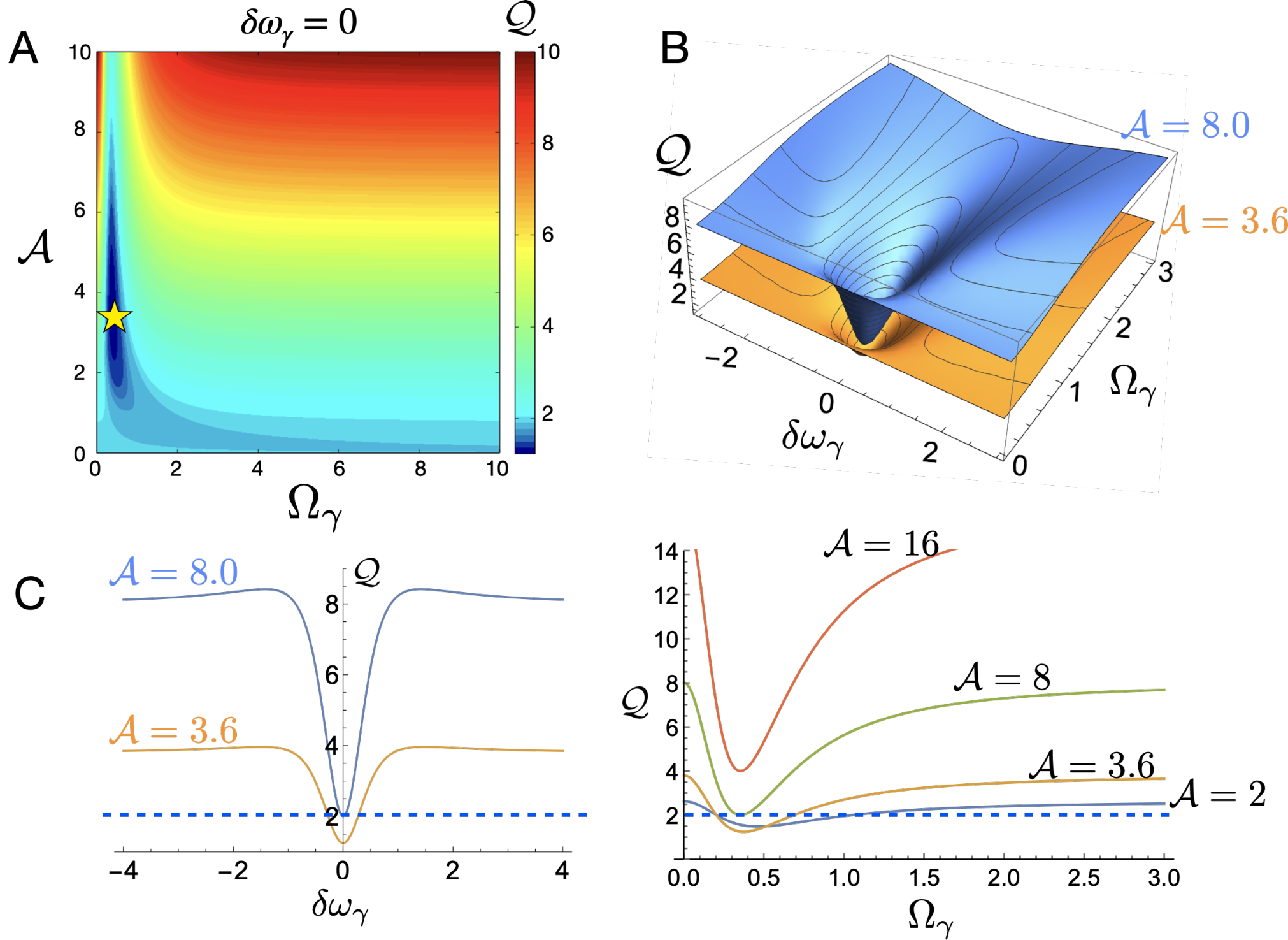
Figure 2: The uncertainty product 𝒬\mathcal{Q}. (A) 𝒬\mathcal{Q} as a function of Ωγ\Omega_{\gamma} and 𝒜\mathcal{A} for the case of perfect resonance (δ​ωγ=0\delta\omega_{\gamma}=0). The condition of (Ωγ,𝒜)(\Omega_{\gamma},\mathcal{A}) that minimizes 𝒬\mathcal{Q} is marked with the star symbol. (B) The diagram of 𝒬=𝒬⁡(Ωγ,δ​ωγ)\mathcal{Q}=\mathcal{Q}(\Omega_{\gamma},\delta\omega_{\gamma}) for 𝒜=3.6\mathcal{A}=3.6 and 𝒜=8\mathcal{A}=8. (C) Dissections of 𝒬\mathcal{Q}. (left) 𝒬⁡(Ωγ=0.37,δ​ωγ)\mathcal{Q}(\Omega_{\gamma}=0.37,\delta\omega_{\gamma}) at 𝒜=3.8\mathcal{A}=3.8 and 8. (right) 𝒬⁡(Ωγ,δ​ωγ=0)\mathcal{Q}(\Omega_{\gamma},\delta\omega_{\gamma}=0) for various values of 𝒜\mathcal{A}. The bound of the original TUR (𝒬=2\mathcal{Q}=2) is marked with the blue dashed line.

V Thermodynamic uncertainty relation

The uncertainty product of TUR at NESS Barato and Seifert 2015; Horowitz and Gingrich 2020 for the net transitions of the TLS is written as

𝒬\displaystyle\mathcal{Q} =limτ→∞Σs​s​τkB​⟨δ​n​(τ)2⟩⟨n⁡(τ)⟩2=(Σs​skB​⟨j⟩)⏟=𝒜​(Var​[j]⟨j⟩)⏟=ℱ\displaystyle=\lim_{\tau\rightarrow\infty}\dfrac{\Sigma^{ss}\tau}{k_{B}}\dfrac{\langle\delta n(\tau)^{2}\rangle}{\langle n(\tau)\rangle^{2}}=\underbrace{\left(\dfrac{\Sigma^{ss}}{k_{B}\langle j\rangle}\right)}_{=\mathcal{A}}\underbrace{\left(\dfrac{\text{Var}[j]}{\langle j\rangle}\right)}_{=\mathcal{F}}
=𝒜​coth⁡(𝒜2)​f​(𝒜,Ωγ,δ​ωγ).\displaystyle=\mathcal{A}\coth{\left(\frac{\mathcal{A}}{2}\right)}f(\mathcal{A},\Omega_{\gamma},\delta\omega_{\gamma}). (15)

The original TUR derived for classical system states that the uncertainty product 𝒬\mathcal{Q} between the cost (Σs​s/kB\Sigma^{ss}/k_{B}) and the precision dictated by the square of the relative fluctuations of current (Var​[j]/⟨j⟩2\text{Var}[j]/\langle j\rangle^{2}) cannot be smaller than 22 Barato and Seifert 2015; Gingrich et al. 2016; Horowitz and Gingrich 2020. However, when TUR is extended to quantum systems, the uncertainty product can have a loose bound. The expression given in Eq. 12 points to the possibility of f⁡(𝒜,Ωγ,δ​ωγ)<1f(\mathcal{A},\Omega_{\gamma},\delta\omega_{\gamma})<1, which in turn leads to 𝒬<2\mathcal{Q}<2, when the imaginary part of coherence is dominant. In fact, ρR=0\rho_{R}=0 for the case of perfect resonance (δ​ωγ=0\delta\omega_{\gamma}=0) simplifies 𝒬\mathcal{Q} to 𝒬⁡(𝒜,Ωγ)=𝒜​coth⁡(𝒜2)​[1−24​Ωγ2(coth2⁡(𝒜2)+8​Ωγ2)2]≥𝒬⁡(𝒜∗,Ωγ∗)≈1.25\mathcal{Q}(\mathcal{A},\Omega_{\gamma})=\mathcal{A}\coth{(\frac{\mathcal{A}}{2})}\left[1-\frac{24\Omega_{\gamma}^{2}}{(\coth^{2}{(\frac{\mathcal{A}}{2})}+8\Omega_{\gamma}^{2})^{2}}\right]\geq\mathcal{Q}(\mathcal{A}^{\ast},\Omega_{\gamma}^{\ast})\approx 1.25 at (𝒜∗,Ωγ∗)≈(3.61,0.37)(\mathcal{A}^{\ast},\Omega_{\gamma}^{\ast})\approx(3.61,0.37) (see Fig. 2A). The minimal uncertainty product, 𝒬≥𝒬min=1.25\mathcal{Q}\geq\mathcal{Q}_{\rm min}=1.25 coincides with the value obtained in a recent work that has studied TUR of a spin in a rotating magnetic field Menczel et al. 2021.

For the case of finite detuning (off-resonance) δ​ωγ≠0\delta\omega_{\gamma}\neq 0, the real part of coherence (ρR≠0\rho_{R}\neq 0) contributes to increasing the size of 𝒬\mathcal{Q} (Fig. 2B, C). Thus, for a given set of parameter (𝒜,Ωγ,δ​ωγ)(\mathcal{A},\Omega_{\gamma},\delta\omega_{\gamma}), the value of 𝒬\mathcal{Q} is determined as a result of competition between the real and imaginary parts of the coherence. Notably, ρR2<3​ρI2\rho_{R}^{2}<3\rho_{I}^{2}, i.e., |δ​ωγ|<(3/2)​coth⁡𝒜2|\delta\omega_{\gamma}|<(\sqrt{3}/2)\coth{\frac{\mathcal{A}}{2}}, is a necessary, but not a sufficient condition for the loose bound of TUR.

TUR can also be recast into the form of an inequality of the Fano factor of transitions Hasegawa and Van Vu 2019. For our system, Eqs. 10 and  11 define the Fano factor of transitions,

ℱ\displaystyle\mathcal{F} =limτ→∞Var​[n​(τ)]⟨n⁡(τ)⟩=Var​[j]⟨j⟩\displaystyle=\lim_{\tau\rightarrow\infty}\frac{\text{Var}[n(\tau)]}{\langle n(\tau)\rangle}=\frac{\text{Var}[j]}{\langle j\rangle}
=coth⁡(𝒜2)​f​(𝒜,Ωγ,δ​ωγ)≥ϕ⁡(𝒜).\displaystyle=\coth{(\frac{\mathcal{A}}{2})}f(\mathcal{A},\Omega_{\gamma},\delta\omega_{\gamma})\geq\phi(\mathcal{A}). (16)

For the original TUR derived for the case of constant driving Barato and Seifert 2015; Gingrich et al. 2016; Horowitz and Gingrich 2020, ϕ⁡(𝒜)=ϕo​(𝒜)=2/𝒜\phi(\mathcal{A})=\phi_{o}(\mathcal{A})=2/\mathcal{A}. For the case of time-symmetric periodic driving, Proesmans and Van den Broeck have shown that the steady state current fluctuations per period in the long-time limit is bounded by Var​[j]/⟨j⟩2≥2​Δ​t/(eΣs​s​Δ​t/kB−1)\text{Var}[j]/\langle j\rangle^{2}\geq 2\Delta t/(e^{\Sigma^{ss}\Delta t/k_{B}}-1) Proesmans and Van den Broeck 2017; Horowitz and Gingrich 2020. Our electromagnetic field-driven quantum TLS is, in principle, under time-symmetric periodic driving with a constant period of Δ​t=2​π/ω\Delta t=2\pi/\omega; however, such a periodicity in driving field under weak field limit (Ω≪ω\Omega\ll\omega) is reduced to a constant driving under RWA, as detailed in Eqs. 6 and 7. Thus, it is pertinent to ask whether or not the uncertainty product of our quantum TLS satisfies the inequality dictated by the classical version of TUR under a constant driving. Since ⟨j⟩​Δ​t=1\langle j\rangle\Delta t=1 from the definition given in Eq. 10 and Σs​s​Δ​t=𝒜\Sigma^{ss}\Delta t=\mathcal{A}, the expression can be cast into Var​[j]/⟨j⟩≥ϕ⁡(𝒜)=ϕp​(𝒜)=2/(e𝒜−1)\text{Var}[j]/\langle j\rangle\geq\phi(\mathcal{A})=\phi_{p}(\mathcal{A})=2/(e^{\mathcal{A}}-1). Mathematically, ϕo​(𝒜)>ϕp​(𝒜)\phi_{o}(\mathcal{A})>\phi_{p}(\mathcal{A}) for all 𝒜≥0\mathcal{A}\geq 0, but ϕp​(𝒜)\phi_{p}(\mathcal{A}) converges to the form of ϕo​(𝒜)\phi_{o}(\mathcal{A}) when 𝒜≪1\mathcal{A}\ll 1.

ℱ\mathcal{F}, plotted against 𝒜\mathcal{A} with randomly varying set of parameters (𝒜,Ωγ,δ​ωγ)(\mathcal{A},\Omega_{\gamma},\delta\omega_{\gamma}), is upper bounded by (5/4)​coth⁡𝒜2(5/4)\coth{\frac{\mathcal{A}}{2}} (the cyan line in Fig. 3), which is obtained from f⁡(𝒜,Ωγ,δ​ωγ)≈1+32​δ​ωγ2​Ωγ2[4​δ​ωγ2+8​Ωγ2]2≤5/4f(\mathcal{A},\Omega_{\gamma},\delta\omega_{\gamma})\approx 1+\frac{32\delta\omega_{\gamma}^{2}\Omega_{\gamma}^{2}}{[4\delta\omega_{\gamma}^{2}+8\Omega_{\gamma}^{2}]^{2}}\leq 5/4 for 𝒜≫1\mathcal{A}\gg 1, |δ​ωγ|≫1|\delta\omega_{\gamma}|\gg 1 and Ωγ≫1\Omega_{\gamma}\gg 1. Of particular note is that there are data points that satisfy ϕp​(𝒜)<ℱ⁡(𝒜,Ωγ,δ​ωγ)<ϕo​(𝒜)\phi_{p}(\mathcal{A})<\mathcal{F}(\mathcal{A},\Omega_{\gamma},\delta\omega_{\gamma})<\phi_{o}(\mathcal{A}) at 1≲𝒜≲61\lesssim\mathcal{A}\lesssim 6, signifying that the TUR of our quantum TLS is characterized with the bound less tight than that of the original TUR (Fig. 3).

Refer to caption
Figure 3: Fano factor (ℱ\mathcal{F}) of a bath-coupled TLS under a weak driving plotted against the net entropy production over a cycle of absorption and emission, 𝒜(=β​ℏ​ω0)\mathcal{A}(=\beta\hbar\omega_{0}). For ℱ\mathcal{F} calculated with a randomly generated set of parameters (𝒜,Ωγ,δ​ωγ)(\mathcal{A},\Omega_{\gamma},\delta\omega_{\gamma}), there are cases whose Fano factor is smaller than the lower bound of the original TUR (blue), but still greater than the bound specified by the generalized uncertainty relation (red) Proesmans and Van den Broeck 2017.

VI Discussions

The relation between the parameters ω\omega, ω0\omega_{0}, γ\gamma, and Ω\Omega,

ω∼ω0≫γ∼Ω\displaystyle\omega\sim\omega_{0}\gg\gamma\sim\Omega (17)

is the essential condition to study the time-irreversible evolution of our TLS. First, for transitions induced by dipole-electric field coupling, Fermi’s golden rule offers an expression for the emission rate, γ=4​ω03​|de​g|2/(3​ℏ​c3)\gamma=4\omega_{0}^{3}|d_{eg}|^{2}/(3\hbar c^{3}) Breuer and Petruccione 2010. Provided that the dipole moment of a molecule (or an atom) is given by |de​g|=e​a0|d_{eg}|=ea_{0} with its electric charge ee and size a0(≲1CLOSEa_{0}(\lesssim 1 nm), and that ω0/c=2​π/λ\omega_{0}/c=2\pi/\lambda where cc is the speed of light, and λ⁡(≈500CLOSE\lambda(\approx 500 nm) is the wavelength of the field in the optical domain, one gets ω0/γ≈6.5×105\omega_{0}/\gamma\approx 6.5\times 10^{5} from γ=(4​α/3)​(2​π​a0/λ)2​ω0\gamma=(4\alpha/3)\left(2\pi a_{0}/\lambda\right)^{2}\omega_{0}, with α≡e2/ℏ​c=1/137\alpha\equiv e^{2}/\hbar c=1/137 and 2​π​a0/λ∼10−22\pi a_{0}/\lambda\sim 10^{-2}. The separation of timescales (ω/γ≫1\omega/\gamma\gg 1) justifies decomposition of the total density matrix into the system and equilibrated bath parts, and rationalizes the truncation of quantum optical master equation at the second order (Born-Markov approximation. See Appendix A). Second, the condition of ω≫Ω\omega\gg\Omega was used in taking the RWA in Eq. 6 to obtain Eq.  7.

Since the Eq. 7 is independent of ω\omega, the system is effectively under a constant driving. As a result, the system at long time limit, if classical, should obey the original TUR Barato and Seifert 2015; Fischer et al. 2020, instead of the generalized TUR under time-symmetric periodic driving Proesmans and Van den Broeck 2017. Thus, the loose TUR bound of our TLS model (𝒬<2\mathcal{Q}<2 in Fig.2) stems from the quantum nature of the dynamics. Our model further elaborates the contribution from the quantum nature to TUR: The imaginary part of quantum coherence contributes to suppressing the Fano factor of net transitions and lowering the TUR bound, whereas the real part of the coherence always tightens the TUR bound. The bound of TUR is determined by the competition between the dissipation and dispersion of the input light source.

For the cases the system-bath coupling (γ\gamma) and/or the strength of driving field (Ω\Omega) are strong and become comparable to the energy scale of the system, one should reevaluate the quantum master equation presented here based on generalized versions of open quantum dynamics that are under active development in recent years Thingna et al. 2012; Tanimura 2020; Ikeda and Sato 2020. However, as long as the energy gap of the TLS is in the optical domain (λ∼500\lambda\sim 500 nm), one of the conditions identified for the loose TUR bound in Fig. 2 (Ωγ≲0.5\Omega_{\gamma}\lesssim 0.5) ensures the relation specified in Eq. 17, which should reduce a generalized quantum master equation into the one studied here. Thus, we anticipate that the condition leading to the loose TUR bound will remain unaltered. Finally, the other condition 𝒜∼(2−8)\mathcal{A}\sim(2-8) (Fig. 2) becomes accessible in the range of high temperature T=(2−8)−1​(h​c/kB​λ)∼𝒪⁡(103)T=(2-8)^{-1}(hc/k_{B}\lambda)\sim\mathcal{O}(10^{3}) K for λ∼500\lambda\sim 500 nm.

Despite the apparent simplicity of the model presented here, it retains all the essential components that enables us to explore the TUR of quantum processes. The model also offers us a physically straightforward understanding of the condition that leads to loosening the TUR bound.

Acknowledgements.
This work was supported by the KIAS Individual Grants CG077602 (D.S.) and CG035003 (C.H.) from the Korea Institute for Advanced Study. We thank the Center for Advanced Computation in KIAS for providing computing resources.

Appendix

VI.1 Derivation of Lindblad dissipator

Introducing the transformations

HI′​(t)\displaystyle H^{\prime}_{I}(t) =eiℏ​Ho​t​HI​(t)​e−iℏ​Ho​t\displaystyle=e^{\frac{i}{\hbar}H_{o}t}H_{I}(t)e^{-\frac{i}{\hbar}H_{o}t}
ρtot′​(t)\displaystyle\rho^{\prime}_{\text{tot}}(t) =eiℏ​Ho​t​ρtot​(t)​e−iℏ​Ho​t\displaystyle=e^{\frac{i}{\hbar}H_{o}t}\rho_{\text{tot}}(t)e^{-\frac{i}{\hbar}H_{o}t} (A1)

with the definitions of

Ho\displaystyle H_{o} ≡HS+HB\displaystyle\equiv H_{S}+H_{B}
HI​(t)\displaystyle H_{I}(t) ≡Hext​(t)+HS​B,\displaystyle\equiv H_{\text{ext}}(t)+H_{SB}, (A2)

one can cast the von Neumann equation into the one in the interaction picture Carmichael 2002

d​ρtot′​(t)d​t=−iℏ​[HI′​(t),ρtot′​(t)].\displaystyle\frac{d\rho^{\prime}_{\text{tot}}(t)}{dt}=-\frac{i}{\hbar}[H^{\prime}_{I}(t),\rho^{\prime}_{\text{tot}}(t)]. (A3)

After integrating Eq.(A3) and expanding it up to the second order, we obtain

d​ρtot′​(t)d​t\displaystyle\frac{d{\rho^{\prime}_{\text{tot}}}(t)}{dt} =−iℏ​[HS​B′​(t),ρtot′​(0)]−iℏ​[Hext′​(t),ρtot′​(0)]\displaystyle=-\frac{i}{\hbar}[H^{\prime}_{SB}(t),\rho^{\prime}_{\text{tot}}(0)]-\frac{i}{\hbar}[H^{\prime}_{\text{ext}}(t),\rho^{\prime}_{\text{tot}}(0)]
−1ℏ2∫0tdt′[HI′(t),[HI′(t′),ρtot′(t′)]].\displaystyle-\frac{1}{\hbar^{2}}\int_{0}^{t}dt^{\prime}[H^{\prime}_{I}(t),[H^{\prime}_{I}(t^{\prime}),\rho^{\prime}_{\text{tot}}(t^{\prime})]]. (A4)

Next, we trace out the bath modes, assuming that the density matrix ρtot​(t)\rho_{\text{tot}}(t) for the total system at time tt can be described with the uncorrelated product state of system (ρ⁡(t)\rho(t)) and environment in equilibrium (ρBe​q\rho_{B}^{eq}), such that ρtot​(t)≈ρ⁡(t)⊗ρBe​q\rho_{\text{tot}}(t)\approx\rho(t)\otimes\rho_{B}^{eq}. Then, it follows that

d​ρ′​(t)d​t=−iℏ​[Hext′​(t),ρ′​(0)]\displaystyle\frac{d{\rho^{\prime}}(t)}{dt}=-\frac{i}{\hbar}[H^{\prime}_{\text{ext}}(t),\rho^{\prime}(0)] −1ℏ2∫0tdt′TrB([Hext′(t),[Hext′(t′),ρ′(t′)⊗ρBe​q]])\displaystyle-\frac{1}{\hbar^{2}}\int_{0}^{t}dt^{\prime}\Tr_{B}\left([H^{\prime}_{\text{ext}}(t),[H^{\prime}_{\text{ext}}(t^{\prime}),\rho^{\prime}(t^{\prime})\otimes\rho_{B}^{eq}]]\right)
−1ℏ2∫0tdt′TrB([HS​B′(t),[HS​B′(t′),ρ′(t′)⊗ρBe​q]]),\displaystyle-\frac{1}{\hbar^{2}}\int_{0}^{t}dt^{\prime}\Tr_{B}\left([H^{\prime}_{SB}(t),[H^{\prime}_{SB}(t^{\prime}),\rho^{\prime}(t^{\prime})\otimes\rho_{B}^{eq}]]\right), (A5)

where ρ′=TrB⁡(ρtot′)\rho^{\prime}=\Tr_{B}\left(\rho^{\prime}_{\text{tot}}\right) was used in the left hand side of the equation and an assumption that the system is decoupled from the environment at t=0t=0 leads to TrB⁡[HS​B′​(t),ρtot′​(0)]=0\Tr_{B}[H^{\prime}_{SB}(t),\rho^{\prime}_{\text{tot}}(0)]=0.

Next, to proceed further, it is convenient to define HS​B=ℏ​∑msm​qmH_{SB}=\hbar\sum\limits_{m}s_{m}q_{m}, where sms_{m} are the system operators and qmq_{m} are the bath operators, with s1≡σ−s_{1}\equiv\sigma_{-}, s2≡σ+s_{2}\equiv\sigma_{+}, q1≡∑k,ξgk,ξ∗​bk,ξ†q_{1}\equiv\sum\limits_{\textbf{k},\xi}g_{\textbf{k},\xi}^{\ast}b_{\textbf{k},\xi}^{\dagger}, and q2≡∑k,ξgk,ξ​bk,ξq_{2}\equiv\sum\limits_{\textbf{k},\xi}g_{\textbf{k},\xi}b_{\textbf{k},\xi}. Then

HS​B′​(t)\displaystyle H^{\prime}_{SB}(t) =ℏ​∑m=1,2eiℏ​(HS+HB)​t​sm​qm​e−iℏ​(HS+HB)​t\displaystyle=\hbar\sum\limits_{m=1,2}e^{\frac{i}{\hbar}(H_{S}+H_{B})t}s_{m}q_{m}e^{-\frac{i}{\hbar}(H_{S}+H_{B})t}
=ℏ​∑m=1,2(eiℏ​HS​t​sm​e−iℏ​HS​t)​(eiℏ​HB​t​qm​e−iℏ​HB​t)\displaystyle=\hbar\sum\limits_{m=1,2}\left(e^{\frac{i}{\hbar}H_{S}t}s_{m}e^{-\frac{i}{\hbar}H_{S}t}\right)\left(e^{\frac{i}{\hbar}H_{B}t}q_{m}e^{-\frac{i}{\hbar}H_{B}t}\right)
=ℏ​∑m=1,2sm​(t)​qm​(t)\displaystyle=\hbar\sum\limits_{m=1,2}s_{m}(t)q_{m}(t) (A6)

where one can show using Baker-Campbell-Hausdorff formula that s1​(t)=σ−​e−i​ω0​ts_{1}(t)=\sigma_{-}e^{-i\omega_{0}t}, s2​(t)=σ+​ei​ω0​ts_{2}(t)=\sigma_{+}e^{i\omega_{0}t}, q1​(t)=∑𝐤,ξg𝐤,ξ∗​b𝐤,ξ†​ei​ω𝐤​tq_{1}(t)=\sum\limits_{{\bf k},\xi}g^{\ast}_{{\bf k},\xi}b^{\dagger}_{{\bf k},\xi}e^{i\omega_{\bf k}t}, and q2​(t)=∑𝐤,ξg𝐤,ξ​b𝐤,ξ​e−i​ω𝐤​tq_{2}(t)=\sum\limits_{{\bf k},\xi}g_{{\bf k},\xi}b_{{\bf k},\xi}e^{-i\omega_{\bf k}t}. The master equation can be written as

d​ρ′​(t)d​t=−iℏ​[Hext′​(t),ρ′​(0)]\displaystyle\frac{d\rho^{\prime}(t)}{dt}=-\frac{i}{\hbar}[H^{\prime}_{\text{ext}}(t),\rho^{\prime}(0)] −1ℏ2∫0tdt′TrB([Hext′(t),[Hext′(t′),ρ′(t′)⊗ρBe​q]])\displaystyle-\frac{1}{\hbar^{2}}\int_{0}^{t}dt^{\prime}\Tr_{B}\left([H^{\prime}_{\text{ext}}(t),[H^{\prime}_{\text{ext}}(t^{\prime}),\rho^{\prime}(t^{\prime})\otimes\rho_{B}^{eq}]]\right)
−1ℏ2∫0tdt′[(s1(t)s2(t′)ρ′(t′)−s2(t′)ρ′(t′)s1(t))⟨q1(t)q2(t′)⟩B\displaystyle-\frac{1}{\hbar^{2}}\int_{0}^{t}dt^{\prime}\left[\left(s_{1}(t)s_{2}(t^{\prime})\rho^{\prime}(t^{\prime})-s_{2}(t^{\prime})\rho^{\prime}(t^{\prime})s_{1}(t)\right)\langle q_{1}(t)q_{2}(t^{\prime})\rangle_{B}\right.
+(s2​(t)​s1​(t′)​ρ′​(t′)−s1​(t′)​ρ′​(t′)​s2​(t))​⟨q2​(t)​q1​(t′)⟩B\displaystyle\left.\qquad\qquad+\left(s_{2}(t)s_{1}(t^{\prime})\rho^{\prime}(t^{\prime})-s_{1}(t^{\prime})\rho^{\prime}(t^{\prime})s_{2}(t)\right)\langle q_{2}(t)q_{1}(t^{\prime})\rangle_{B}\right.
+(ρ′​(t′)​s1​(t′)​s2​(t)−s2​(t)​ρ′​(t′)​s1​(t′))​⟨q1​(t′)​q2​(t)⟩B\displaystyle\left.\qquad\qquad+\left(\rho^{\prime}(t^{\prime})s_{1}(t^{\prime})s_{2}(t)-s_{2}(t)\rho^{\prime}(t^{\prime})s_{1}(t^{\prime})\right)\langle q_{1}(t^{\prime})q_{2}(t)\rangle_{B}\right.
+(ρ′(t′)s2(t′)s1(t)−s1(t)ρ′(t′)s2(t′))⟨q2(t′)q1(t)⟩B],\displaystyle\left.\qquad\qquad+\left(\rho^{\prime}(t^{\prime})s_{2}(t^{\prime})s_{1}(t)-s_{1}(t)\rho^{\prime}(t^{\prime})s_{2}(t^{\prime})\right)\langle q_{2}(t^{\prime})q_{1}(t)\rangle_{B}\right], (A7)

where ⟨qm​(t)​qn​(t′)⟩B=TrB​[ρBe​q​qm​(t)​qn​(t′)]\langle q_{m}(t)q_{n}(t^{\prime})\rangle_{B}=\text{Tr}_{B}\left[\rho_{B}^{eq}q_{m}(t)q_{n}(t^{\prime})\right] represents the bath correlation function. For example,

⟨q1​(t)​q2​(t′)⟩B\displaystyle\langle q_{1}(t)q_{2}(t^{\prime})\rangle_{B} =∑𝐤,ξ∑𝐤′,ξ′g𝐤,ξ∗​g𝐤′,ξ′​ei​ω𝐤​t​e−i​ω𝐤′​t′​TrB​(ρBe​q​b𝐤,ξ†​b𝐤′,ξ′)\displaystyle=\sum_{{\bf k},\xi}\sum_{{\bf k}^{\prime},\xi^{\prime}}g_{{\bf k},\xi}^{\ast}g_{{\bf k}^{\prime},\xi^{\prime}}e^{i\omega_{\bf k}t}e^{-i\omega_{{\bf k}^{\prime}}t^{\prime}}\text{Tr}_{B}(\rho_{B}^{eq}b_{{\bf k},\xi}^{\dagger}b_{{\bf k}^{\prime},\xi^{\prime}})
=∑𝐤|g𝐤,ξ|2​ei​ω𝐤​(t−t′)​n¯​(ω𝐤).\displaystyle=\sum_{{\bf k}}|g_{{\bf k},\xi}|^{2}e^{i\omega_{\bf k}(t-t^{\prime})}\bar{n}(\omega_{\bf k}). (A8)

Likewise

⟨q2​(t)​q1​(t′)⟩B=∑𝐤|g𝐤|2​e−i​ω𝐤​(t−t′)​(n¯​(ω𝐤)+1).\displaystyle\langle q_{2}(t)q_{1}(t^{\prime})\rangle_{B}=\sum_{{\bf k}}|g_{{\bf k}}|^{2}e^{-i\omega_{\bf k}(t-t^{\prime})}(\bar{n}(\omega_{\bf k})+1). (A9)

By substituting s1,2s_{1,2}, q1,2q_{1,2} back, and transforming the time u=t−t′u=t-t^{\prime}, we obtain

d​ρ′​(t)d​t=−iℏ​[Hext′​(t),ρ′​(0)]\displaystyle\frac{d\rho^{\prime}(t)}{dt}=-\frac{i}{\hbar}[H^{\prime}_{\text{ext}}(t),\rho^{\prime}(0)] −1ℏ2∫0tdt′TrB([Hext′(t),[Hext′(t′),ρ′(t′)⊗ρBe​q]])\displaystyle-\frac{1}{\hbar^{2}}\int_{0}^{t}dt^{\prime}\Tr_{B}\left([H^{\prime}_{\text{ext}}(t),[H^{\prime}_{\text{ext}}(t^{\prime}),\rho^{\prime}(t^{\prime})\otimes\rho_{B}^{eq}]]\right)
−∑𝐤,ξ|g𝐤,ξ|2∫0tdu[(σ−σ+ρ′(t−u)−σ+ρ′(t−u)σ−)ei⁡(ω𝐤−ω0)​un¯(ω𝐤)\displaystyle-\sum_{{\bf k},\xi}|g_{{\bf k},\xi}|^{2}\int_{0}^{t}du\left[\left(\sigma_{-}\sigma_{+}\rho^{\prime}(t-u)-\sigma_{+}\rho^{\prime}(t-u)\sigma_{-}\right)e^{i(\omega_{\bf k}-\omega_{0})u}\bar{n}(\omega_{\bf k})\right.
+(σ+​σ−​ρ′​(t−u)−σ−​ρ′​(t−u)​σ+)​e−i⁡(ω𝐤−ω0)​u​(n¯​(ω𝐤)+1)\displaystyle\left.\qquad\qquad+\left(\sigma_{+}\sigma_{-}\rho^{\prime}(t-u)-\sigma_{-}\rho^{\prime}(t-u)\sigma_{+}\right)e^{-i(\omega_{\bf k}-\omega_{0})u}(\bar{n}(\omega_{\bf k})+1)\right.
+(ρ′​(t−u)​σ−​σ+−σ+​ρ′​(t−u)​σ−)​e−i⁡(ω𝐤−ω0)​u​n¯​(ω𝐤)\displaystyle\left.\qquad\qquad+\left(\rho^{\prime}(t-u)\sigma_{-}\sigma_{+}-\sigma_{+}\rho^{\prime}(t-u)\sigma_{-}\right)e^{-i(\omega_{\bf k}-\omega_{0})u}\bar{n}(\omega_{\bf k})\right.
+(ρ′(t−u)σ+σ−−σ−ρ′(t−u)σ+)ei⁡(ω𝐤−ω0)​u(n¯(ω𝐤)+1)].\displaystyle\left.\qquad\qquad+\left(\rho^{\prime}(t-u)\sigma_{+}\sigma_{-}-\sigma_{-}\rho^{\prime}(t-u)\sigma_{+}\right)e^{i(\omega_{\bf k}-\omega_{0})u}(\bar{n}(\omega_{\bf k})+1)\right]. (A10)

To proceed further, Markov approximation is often considered with ρ′​(t−u)→ρ′​(t)\rho^{\prime}(t-u)\rightarrow\rho^{\prime}(t) and ∫0t𝑑u→∫0∞𝑑u\int_{0}^{t}du\rightarrow\int_{0}^{\infty}du by assuming that the value of density matrix is determined without memory, and limt→∞∫−ttd​u​∑𝐤,ξ|g𝐤,ξ|2​e±i⁡(ω𝐤−ω0)​u→γ≡2​π​∫d3​k​J​(𝐤)​|g𝐤,ξ|2​δ​(ω𝐤−ω0)\lim_{t\rightarrow\infty}\int_{-t}^{t}du\sum_{{\bf k},\xi}|g_{{\bf k},\xi}|^{2}e^{\pm i(\omega_{\bf k}-\omega_{0})u}\rightarrow\gamma\equiv 2\pi\int d^{3}kJ({\bf k})|g_{{\bf k},\xi}|^{2}\delta(\omega_{\bf k}-\omega_{0}) where J⁡(𝐤)J({\bf k}) is the spectral density, determining the decay rate γ\gamma Carmichael 2002.

Transformed back to the Schrödinger picture, the master equation takes the following form Carmichael 2002

d​ρ​(t)d​t=−iℏ​[HS+Hext​(t),ρ⁡(t)]+𝒟⁡(ρ⁡(t))\displaystyle\frac{d\rho(t)}{dt}=-\frac{i}{\hbar}[H_{S}+H_{\text{ext}}(t),\rho(t)]+\mathcal{D}(\rho(t)) (A11)

with the Lindblad dissipator

𝒟⁡(ρ)\displaystyle\mathcal{D}(\rho) =γ2​(n¯+1)​(2​σ−​ρ​σ+−σ+​σ−​ρ−ρ​σ+​σ−)\displaystyle=\dfrac{\gamma}{2}(\bar{n}+1)\left(2\sigma_{-}\rho\sigma_{+}-\sigma_{+}\sigma_{-}\rho-\rho\sigma_{+}\sigma_{-}\right)
+γ2​n¯​(2​σ+​ρ​σ−−σ−​σ+​ρ−ρ​σ−​σ+),\displaystyle+\dfrac{\gamma}{2}\bar{n}\left(2\sigma_{+}\rho\sigma_{-}-\sigma_{-}\sigma_{+}\rho-\rho\sigma_{-}\sigma_{+}\right), (A12)

where n¯=n¯​(ω0)=(eβ​ℏ​ω0−1)−1\bar{n}=\bar{n}(\omega_{0})=(e^{\beta\hbar\omega_{0}}-1)^{-1} is the average number of thermal photons.

VI.2 Transformation to the rotating frame

The density matrix ρ~=|ϕ⟩​⟨ϕ|\tilde{\rho}=\ket{\phi}\bra{\phi} in the rotating frame is transformed into the one in the stationary frame ρ=|ψ⟩​⟨ψ|\rho=\ket{\psi}\bra{\psi} via the following operation,

|ψ⟩​⟨ψ|⏟=ρ=e−iωtσz/2|ϕ⟩​⟨ϕ|⏟=ρ~ei​ω​t​σz/2,\underbrace{\ket{\psi}\bra{\psi}}_{=\rho}=e^{-i\omega t\sigma_{z}/2}\underbrace{\ket{\phi}\bra{\phi}}_{=\tilde{\rho}}e^{i\omega t\sigma_{z}/2}, (B1)

which allows us to express the excited state population in the stationary frame into the one in the rotating frame as

ρ~e​e=ei​ω​t​σz/2|e⟩​⟨e|⏟=ρe​ee−iωtσz/2.\tilde{\rho}_{ee}=e^{i\omega t\sigma_{z}/2}\underbrace{\ket{e}\bra{e}}_{=\rho_{ee}}e^{-i\omega t\sigma_{z}/2}. (B2)

Employing the Baker-Campbell-Hausdorff formula, es​A^​B^​e−s​A^=B^+(s/1!)​[A^,B^]+(s2/2!)​[A^,[A^,B^]]+⋯e^{s\hat{A}}\hat{B}e^{-s\hat{A}}=\hat{B}+(s/1!)[\hat{A},\hat{B}]+(s^{2}/2!)[\hat{A},[\hat{A},\hat{B}]]+\cdots, one can show that ρ~e​e=ρe​e\tilde{\rho}_{ee}=\rho_{ee}, ρ~g​g=ρg​g\tilde{\rho}_{gg}=\rho_{gg}, ρ~e​g=ρe​g​ei​ω​t\tilde{\rho}_{eg}=\rho_{eg}e^{i\omega t}, and ρ~g​e=ρg​e​e−i​ω​t\tilde{\rho}_{ge}=\rho_{ge}e^{-i\omega t}.

Refer to caption
Figure 4: The susceptibility of the system as a function of scaled detuning (δ​ωγ\delta\omega_{\gamma}) calculated at Ωγ=0.5\Omega_{\gamma}=0.5 and 𝒜=β​ℏ​ω0=2\mathcal{A}=\beta\hbar\omega_{0}=2. (A) the absorption profile (i.e., χ′′\chi^{\prime\prime}) of the TLS. (B) the dispersion profile (i.e., χ′\chi^{\prime}) of the medium.

VI.3 Relation between the coherence and dielectric susceptibility

Inside a dielectric medium, the electric polarization, defined as the total dipole moment per volume, i.e., P→=N​⟨d→⟩\vec{P}=N\langle\vec{d}\rangle with NN the number of molecules per volume, is induced by the incident radiation field, i.e., P→=χ​E→\vec{P}=\chi\vec{E}, where χ\chi is the linear susceptibility of the medium Scully and Zubairy 1997. With ⟨d→⟩=Tr​(ρ~​d→)=ρ~e​g​d→g​e+ρ~g​e​d→e​g=ei​ω​t​(ρe​g​d→g​e+ρg​e​d→e​g​e−2​i​ω​t)≈ρ~e​g​d→g​e\langle\vec{d}\rangle=\text{Tr}(\tilde{\rho}\vec{d})=\tilde{\rho}_{eg}\vec{d}_{ge}+\tilde{\rho}_{ge}\vec{d}_{eg}=e^{i\omega t}(\rho_{eg}\vec{d}_{ge}+\rho_{ge}\vec{d}_{eg}e^{-2i\omega t})\approx\tilde{\rho}_{eg}\vec{d}_{ge}, the susceptibility can be expressed as χ=Nd​ρ~e​g\chi=N_{d}\tilde{\rho}_{eg} with Nd=N​|dg​e|/|ε→|N_{d}=N|d_{ge}|/|\vec{\varepsilon}|. In the light-matter interactions, the properties of the medium can be investigated by studying χ\chi, which is decomposed into the real (χ′\chi^{\prime}) and imaginary part (χ′′\chi^{\prime\prime}), i.e., χ=χ′+i​χ′′\chi=\chi^{\prime}+i\chi^{\prime\prime}. For the medium with |χ|≪1|\chi|\ll 1, since the refractive index (n¯\underline{n}) is related with the dielectric constant as n¯2=ϵ=1+4​π​χ\underline{n}^{2}=\epsilon=1+4\pi\chi (in Gaussian units),

n¯≈1+2​π​χ′.\displaystyle\underline{n}\approx 1+2\pi\chi^{\prime}. (C1)

The incident radiation field is absorbed to the medium is quantified by the attenuation coefficient α\alpha, which is related to the wave vector as k=β+i​α/2k=\beta+i\alpha/2, which leads to E→∼ei​k​z∼ei​β​z−α​z/2\vec{E}\sim e^{ikz}\sim e^{i\beta z-\alpha z/2} and |E→|2∼e−α​z|\vec{E}|^{2}\sim e^{-\alpha z}. From k=(ω/c)​n¯=(ω/c)​1+4​π​χ′+4​π​i​χ′′≈(ω/c)​(1+2​π​χ′+2​π​i​χ′′)k=(\omega/c)\underline{n}=(\omega/c)\sqrt{1+4\pi\chi^{\prime}+4\pi i\chi^{\prime\prime}}\approx(\omega/c)(1+2\pi\chi^{\prime}+2\pi i\chi^{\prime\prime}), it follows that

α=4​π​(ωc)​χ′′.\displaystyle\alpha=4\pi\left(\frac{\omega}{c}\right)\chi^{\prime\prime}. (C2)

This implies that the real part of the susceptibility (i.e., χ′=Nd​ρ~R\chi^{\prime}=N_{d}\tilde{\rho}_{R}) informs about the dispersion profile of the medium, while the imaginary part of the susceptibility (i.e., χ′′=Nd​ρ~I\chi^{\prime\prime}=N_{d}\tilde{\rho}_{I}) describes the absorption profile of the medium.

The degree of the absorption and dispersion varies with detuning of the field (Fig. 4). For the perfect resonance (i.e., when δ​ω=0\delta\omega=0) the excitation is completely absorbed by the medium (χ′′\chi^{\prime\prime} maximized in Fig. 4) without any dispersion (χ′=0\chi^{\prime}=0 in Fig. 4). With increasing |δ​ω||\delta\omega|, the absorption (dispersion) in the medium decreases (increases).

VI.4 Method of generating function

The dynamical equations (Eq. 7) can be cast into the matrix form,

∂τρ~​(τ)=ℒ​ρ~​(τ).\displaystyle\partial_{\tau}\tilde{\rho}(\tau)=\mathcal{L}\tilde{\rho}(\tau). (D1)

where ρ~=(ρ~e​e,ρ~e​g,ρ~g​e,ρ~g​g)T\tilde{\rho}=(\tilde{\rho}_{ee},\tilde{\rho}_{eg},\tilde{\rho}_{ge},\tilde{\rho}_{gg})^{T} is a vector in Liouville space, and ℒ\mathcal{L} denotes the 4×44\times 4 Liouvillian super-operator. We aim to count the net number of photon transfer to the surrounding bath for time interval τ\tau (n⁡(τ)n(\tau)) and calculate its mean current and current fluctuations at steady state. Since the light-induced absorption and emission is a cyclic process for the system, we assume that the system is periodic in state space and that the superoperator ℒ\mathcal{L} is periodic with its period by L(=4)L(=4), satisfying ℒi​j=ℒi+L,j+L\mathcal{L}_{ij}=\mathcal{L}_{i+L,j+L} for all ii, j=0j=0, 11, 22, 33 representing the quantum state e​eee, e​geg, g​ege, g​ggg, respectively, and introduce a generalized coordinate μ∈ℤ\mu\in\mathbb{Z}, which is related with the numeric index i=0i=0, 11, 22, 33 as μ=i (mod L) with L=4\mu=i\text{ }(\text{mod}\text{ }L)\text{ with }L=4. This allows us to count the cycles of absorptions followed by emissions via ρ~i​(μ,τ)≡ρ~​(μ,τ)​δμ,iL\tilde{\rho}_{i}(\mu,\tau)\equiv\tilde{\rho}(\mu,\tau)\delta_{\mu,i}^{L} with the generalized Kronecker delta, δμ,iL=1\delta_{\mu,i}^{L}=1 if μ=i\mu=i (mod LL) and δμ,iL=0\delta_{\mu,i}^{L}=0 otherwise  Koza 1999; Bruderer et al. 2014. Here, ρ~i​(μ,τ)\tilde{\rho}_{i}(\mu,\tau) denotes the probability of finding a system at a given quantum state i∈{e​e,e​g,g​e,g​g}i\in\{ee,eg,ge,gg\} at site μ\mu at time τ\tau.

We consider a generating function for each element ρ~i\tilde{\rho}_{i} of the vector ρ~\tilde{\rho},

𝒢i​(z,τ)=∑μ=−∞∞ez​nμ​ρ~i​(μ,τ).\displaystyle\mathcal{G}_{i}(z,\tau)=\sum_{\mu=-\infty}^{\infty}e^{zn_{\mu}}\tilde{\rho}_{i}(\mu,\tau). (D2)

Multiplying the factor ez​nμe^{zn_{\mu}} to both sides of a generalized version of Eq. D1, namely ∂τρ~i​(μ,τ)=∑jℒi​j​ρ~j​(μ,τ)\partial_{\tau}\tilde{\rho}_{i}(\mu,\tau)=\sum_{j}\mathcal{L}_{ij}\tilde{\rho}_{j}(\mu,\tau), and summing over μ\mu, one gets

∂τ𝒢i​(z,τ)=∑j[Γ⁡(z)]i​j​𝒢j​(z,τ)\displaystyle\partial_{\tau}\mathcal{G}_{i}(z,\tau)=\sum_{j}[\Gamma(z)]_{ij}\mathcal{G}_{j}(z,\tau) (D3)

where

Γ⁡(z)\displaystyle\Gamma(z) ≡[−(n¯+1)−i​Ωγi​Ωγn¯​e−z−i​Ωγi​δ​ωγ−(2​n¯+1)/20i​Ωγi​Ωγ0−i​δ​ωγ−(2​n¯+1)/2−i​Ωγ(n¯+1)​ezi​Ωγ−i​Ωγ−n¯].\displaystyle\equiv\begin{bmatrix}-(\bar{n}+1)&-i\Omega_{\gamma}&i\Omega_{\gamma}&\bar{n}e^{-z}\\ -i\Omega_{\gamma}&i\delta\omega_{\gamma}-(2\bar{n}+1)/2&0&i\Omega_{\gamma}\\ i\Omega_{\gamma}&0&-i\delta\omega_{\gamma}-(2\bar{n}+1)/2&-i\Omega_{\gamma}\\ (\bar{n}+1)e^{z}&i\Omega_{\gamma}&-i\Omega_{\gamma}&-\bar{n}\end{bmatrix}. (D4)

In obtaining the matrix Γ⁡(z)\Gamma(z) where the factor ez​nμe^{zn_{\mu}} is multiplied to each element, we have set nμ=−1n_{\mu}=-1 for the matrix element [Γ⁡(z)]e​e,g​g[\Gamma(z)]_{ee,gg} corresponding to absorption, nμ=1n_{\mu}=1 for [Γ⁡(z)]g​g,e​e[\Gamma(z)]_{gg,ee} corresponding to emission, and nμ=0n_{\mu}=0 for the rest. The formal solution of Eq. D3 can be written as

𝒢i​(z,τ)=∑αTα​i​(z)​eλα​(z)​τ\displaystyle\mathcal{G}_{i}(z,\tau)=\sum_{\alpha}T_{\alpha i}(z)e^{\lambda_{\alpha}(z)\tau} (D5)

where λα​(z)\lambda_{\alpha}(z) and Tα​i​(z)T_{\alpha i}(z) are the α\alpha-th eigenvalue and the corresponding eigenstate of Γ⁡(z)\Gamma(z), satisfying ∑j[Γ⁡(z)]i​j​Tα​j=λα​(z)​Tα​i​(z)\sum_{j}\left[\Gamma(z)\right]_{ij}T_{\alpha j}=\lambda_{\alpha}(z)T_{\alpha i}(z) with λ0​(z)>λ1​(z)>λ2​(z)>λ3​(z)\lambda_{0}(z)>\lambda_{1}(z)>\lambda_{2}(z)>\lambda_{3}(z) (α=0,1,2,3\alpha=0,1,2,3). At steady state, 𝒢i​(z,τ)\mathcal{G}_{i}(z,\tau) is dominated by the term with the largest eigenvalue

limτ→∞𝒢i​(z,τ)∼T0​i​(z,τ)​eλ0​(z)​τ.\displaystyle\lim_{\tau\rightarrow\infty}\mathcal{G}_{i}(z,\tau)\sim T_{0i}(z,\tau)e^{\lambda_{0}(z)\tau}. (D6)

The eigenvalues λα​(z)\lambda_{\alpha}(z) of Γ⁡(z)\Gamma(z) are obtained from the characteristic polynomial

det⁡|λ⁡(z)​ℐ−Γ⁡(z)|=∑n=04an​(z)​λn​(z)=0,\displaystyle\det|\lambda(z)\mathcal{I}-\Gamma(z)|=\sum_{n=0}^{4}a_{n}(z)\lambda^{n}(z)=0, (D7)

where

a4\displaystyle a_{4} =1\displaystyle=1
a3\displaystyle a_{3} =2​(2​n¯+1)\displaystyle=2(2\bar{n}+1)
a2\displaystyle a_{2} =14​[5​(2​n¯+1)2+4​δ​ωγ2+16​Ωγ2]\displaystyle=\frac{1}{4}\left[5(2\bar{n}+1)^{2}+4\delta\omega_{\gamma}^{2}+16\Omega_{\gamma}^{2}\right]
a1​(z)\displaystyle a_{1}(z) =14​[(2​n¯+1)3+4​δ​ωγ2​(2​n¯+1)+16​Ωγ2​(2​n¯+1)−8​Ωγ2​(ez+n¯​e−z+n¯​ez)]\displaystyle=\frac{1}{4}\left[(2\bar{n}+1)^{3}+4\delta\omega_{\gamma}^{2}(2\bar{n}+1)+16\Omega_{\gamma}^{2}(2\bar{n}+1)-8\Omega_{\gamma}^{2}\left(e^{z}+\bar{n}e^{-z}+\bar{n}e^{z}\right)\right]
a0​(z)\displaystyle a_{0}(z) =−Ωγ2​[ez+n¯​e−z+2​n¯2​e−z+3​n¯​ez+2​n¯2​ez−(2​n¯+1)2].\displaystyle=-\Omega_{\gamma}^{2}\left[e^{z}+\bar{n}e^{-z}+2\bar{n}^{2}e^{-z}+3\bar{n}e^{z}+2\bar{n}^{2}e^{z}-(2\bar{n}+1)^{2}\right].

Now, summing 𝒢i​(z,τ)\mathcal{G}_{i}(z,\tau) over the index i∈{e​e,e​g,g​e,g​g}i\in\{ee,eg,ge,gg\}, we obtain the following expression that can be used as the moment generating function:

𝒢⁡(z,τ)≡∑i𝒢i​(z,τ)=∑i∑μ=−∞∞ez​nμ​ρ~i​(μ,τ)\displaystyle\mathcal{G}(z,\tau)\equiv\sum_{i}\mathcal{G}_{i}(z,\tau)=\sum_{i}\sum_{\mu=-\infty}^{\infty}e^{zn_{\mu}}\tilde{\rho}_{i}(\mu,\tau) (D8)

which allows us to calculate the first and second cumulant of n⁡(τ)n(\tau) as follows.

⟨n⁡(τ)⟩=∑i∑μnμ​ρ~i​(μ,τ)∑i∑μρ~i​(μ,τ)=∂zlog⁡(𝒢⁡(z,τ))|z=0\displaystyle\langle n(\tau)\rangle=\frac{\sum_{i}\sum_{\mu}n_{\mu}\tilde{\rho}_{i}(\mu,\tau)}{\sum_{i}\sum_{\mu}\tilde{\rho}_{i}(\mu,\tau)}=\partial_{z}\log{\mathcal{G}(z,\tau)}|_{z=0} (D9)

and

⟨n​(τ)2⟩−⟨n⁡(τ)⟩2=∂z2log⁡(𝒢⁡(z,τ))|z=0.\displaystyle\langle n(\tau)^{2}\rangle-\langle n(\tau)\rangle^{2}=\partial_{z}^{2}\log{\mathcal{G}(z,\tau)}|_{z=0}. (D10)

Finally, from Eqs. D9 and D10, and the asymptotic expression of 𝒢⁡(z,τ)\mathcal{G}(z,\tau),

limτ→∞𝒢⁡(z,τ)∼h0​(z,τ)​eλ0​(z)​τ.\displaystyle\lim_{\tau\rightarrow\infty}\mathcal{G}(z,\tau)\sim h_{0}(z,\tau)e^{\lambda_{0}(z)\tau}. (D11)

with h0​(z,τ)≡∑iT0​i​(z,τ)h_{0}(z,\tau)\equiv\sum_{i}T_{0i}(z,\tau), we can obtain ⟨j⟩\langle j\rangle and Var​[j]\text{Var}[j],

⟨j⟩≡limτ→∞⟨n⁡(τ)⟩τ=λ0′​(0)\displaystyle\langle j\rangle\equiv\lim_{\tau\rightarrow\infty}\frac{\langle n(\tau)\rangle}{\tau}=\lambda_{0}^{\prime}(0) (D12)

and

Var​[j]≡limτ→∞⟨n​(τ)2⟩−⟨n⁡(τ)⟩2τ=λ0′′​(0).\displaystyle\text{Var}[j]\equiv\lim_{\tau\rightarrow\infty}\frac{\langle n(\tau)^{2}\rangle-\langle n(\tau)\rangle^{2}}{\tau}=\lambda_{0}^{\prime\prime}(0). (D13)

These key values of λ0′​(0)\lambda^{\prime}_{0}(0) and λ0′′​(0)\lambda^{\prime\prime}_{0}(0) can be evaluated in terms of the coefficients of the characteristic polynomial (Eq. D7) differentiated with respect to zz at z=0z=0 as follows:

a0′​(0)+a1​(0)​λ0′​(0)=0\displaystyle a_{0}^{\prime}(0)+a_{1}(0)\lambda_{0}^{\prime}(0)=0 (D14)

and

a0′′​(0)+2​a1′​(0)​λ0′​(0)+a1​(0)​λ0′′​(0)+2​a2​(0)​(λ0′​(0))2=0.\displaystyle a_{0}^{\prime\prime}(0)+2a_{1}^{\prime}(0)\lambda_{0}^{\prime}(0)+a_{1}(0)\lambda_{0}^{\prime\prime}(0)+2a_{2}(0)(\lambda_{0}^{\prime}(0))^{2}=0. (D15)

Therefore,

⟨j⟩=λ0′​(0)=−a0′​(0)a1​(0)\displaystyle\langle j\rangle=\lambda_{0}^{\prime}(0)=-\frac{a_{0}^{\prime}(0)}{a_{1}(0)} (D16)

and

Var​[j]=λ0′′​(0)\displaystyle\text{Var}[j]=\lambda_{0}^{\prime\prime}(0)
=−1a1​(0)​(a0′′​(0)+2​a1′​(0)​λ0′​(0)+2​a2​(0)​(λ0′​(0))2).\displaystyle=-\frac{1}{a_{1}(0)}\left(a_{0}^{\prime\prime}(0)+2a_{1}^{\prime}(0)\lambda_{0}^{\prime}(0)+2a_{2}(0)(\lambda_{0}^{\prime}(0))^{2}\right). (D17)

References

  • Barato and Seifert (2015) A. C. Barato and U. Seifert, Thermodynamic Uncertainty Relation for Biomolecular Processes, Phys. Rev. Lett. 114, 158101 (2015).
  • Gingrich et al. (2016) T. R. Gingrich, J. M. Horowitz, N. Perunov, and J. L. England, Dissipation Bounds All Steady-State Current Fluctuations, Phys. Rev. Lett. 116, 120601 (2016).
  • Dechant and Sasa (2018a) A. Dechant and S.-i. Sasa, Entropic bounds on currents in langevin systems, Phys. Rev. E 97, 062101 (2018a).
  • Horowitz and Gingrich (2020) J. M. Horowitz and T. R. Gingrich, Thermodynamic uncertainty relations constrain non-equilibrium fluctuations, Nature Physics 16, 15 (2020).
  • Pietzonka et al. (2017) P. Pietzonka, F. Ritort, and U. Seifert, Finite-time generalization of the thermodynamic uncertainty relation, Phys. Rev. E. 96, 012101 (2017).
  • Horowitz and Gingrich (2017) J. M. Horowitz and T. R. Gingrich, Proof of the finite-time thermodynamic uncertainty relation for steady-state currents, Phys. Rev. E 96, 020103(R) (2017).
  • Dechant and Sasa (2018b) A. Dechant and S.-i. Sasa, Current fluctuations and transport efficiency for general langevin systems, J. Stat. Mech. , 063209 (2018b).
  • Proesmans and Van den Broeck (2017) K. Proesmans and C. Van den Broeck, Discrete-Time Thermodynamic-like Uncertainty Relation, EPL 119, 20001 (2017).
  • Pietzonka et al. (2016) P. Pietzonka, A. C. Barato, and U. Seifert, Universal bound on the efficiency of molecular motors, J. Stat. Mech. Theory Exp. , 124004 (2016).
  • Hwang and Hyeon (2018) W. Hwang and C. Hyeon, Energetic Costs, Precision, and Transport Efficiency of Molecular Motors, J. Phys. Chem. Lett. 9, 513 (2018).
  • Marsland III et al. (2019) R. Marsland III, W. Cui, and J. M. Horowitz, The thermodynamic uncertainty relation in biochemical oscillations, J. Roy. Soc. Interface 16, 20190098 (2019).
  • Song and Hyeon (2020) Y. Song and C. Hyeon, Thermodynamic cost, speed, fluctuations, and error reduction of biological copy machines, J. Phys. Chem. Lett. 11, 3136 (2020).
  • Mugnai et al. (2020) M. L. Mugnai, C. Hyeon, M. Hinczewski, and D. Thirumalai, Theoretical perspectives on biological machines, Rev. Mod. Phys. 92, 025001 (2020).
  • Kim and Hyeon (2021) P. Kim and C. Hyeon, Thermodynamic optimality of glycolytic oscillations, J. Phys. Chem. B 154, 214901 (2021).
  • Song and Hyeon (2021) Y. Song and C. Hyeon, Thermodynamic uncertainty relation to assess biological processes, J. Chem. Phys. 154, 130901 (2021).
  • Dechant (2018) A. Dechant, Multidimensional thermodynamic uncertainty relations, J. Phys. A: Math. Theor. 52, 035001 (2018).
  • Pietzonka and Seifert (2018) P. Pietzonka and U. Seifert, Universal Trade-Off between Power, Efficiency, and Constancy in Steady-State Heat Engines, Phys. Rev. Lett. 120, 190602 (2018).
  • Holubec and Ryabov (2018) V. Holubec and A. Ryabov, Cycling Tames Power Fluctuations near Optimum Efficiency, Phys. Rev. Lett. 121, 120601 (2018).
  • Dechant and Sasa (2018c) A. Dechant and S.-i. Sasa, Current fluctuations and transport efficiency for general Langevin systems, J. Stat. Mech. 2018, 063209 (2018c).
  • Pigolotti et al. (2017) S. Pigolotti, I. Neri, E. Roldan, and F. Julicher, Generic Properties of Stochastic Entropy Production, Phys. Rev. Lett. 119, 140604 (2017).
  • Hyeon and Hwang (2017) C. Hyeon and W. Hwang, Physical insight into the thermodynamic uncertainty relation using Brownian motion in tilted periodic potentials, Phys. Rev. E 96, 012156 (2017).
  • Brandner et al. (2018) K. Brandner, T. Hanazato, and K. Saito, Thermodynamic Bounds on Precision in Ballistic Multiterminal Transport, Phys. Rev. Lett. 120, 090601 (2018).
  • Lee et al. (2018) S. Lee, C. Hyeon, and J. Jo, Thermodynamic uncertainty relation of interacting oscillators in synchrony, Phys. Rev. E 98, 032119 (2018).
  • Li et al. (2019) J. Li, J. M. Horowitz, T. R. Gingrich, and N. Fakhri, Quantifying dissipation using fluctuating currents, Nature Commun. 10, 1666 (2019).
  • Macieszczak et al. (2018) K. Macieszczak, K. Brandner, and J. P. Garrahan, Unified Thermodynamic Uncertainty Relations in Linear Response, Phys. Rev. Lett. 121, 130601 (2018).
  • Timpanaro et al. (2019) A. M. Timpanaro, G. Guarnieri, J. Goold, and G. T. Landi, Thermodynamic Uncertainty Relations from Exchange Fluctuation Theorems, Phys. Rev. Lett. 123, 090604 (2019).
  • Chiuchiu and Pigolotti (2018) D. Chiuchiu and S. Pigolotti, Mapping of uncertainty relations between continuous and discrete time, Phys. Rev. E 97, 032109 (2018).
  • Koyuk et al. (2019) T. Koyuk, U. Seifert, and P. Pietzonka, A generalization of the thermodynamic uncertainty relation to periodically driven systems, J. Phys. A: Math. Theor. 52, 02LT02 (2019).
  • Barato et al. (2018) A. C. Barato, R. Chetrite, A. Faggionato, and D. Gabrielli, Bounds on current fluctuations in periodically driven systems, New J. Phys. 20, 103023 (2018).
  • Hasegawa and Van Vu (2019) Y. Hasegawa and T. Van Vu, Fluctuation theorem uncertainty relation, Phys. Rev. Lett. 123, 110602 (2019).
  • Fischer et al. (2020) L. P. Fischer, H.-M. Chun, and U. Seifert, Free diffusion bounds the precision of currents in underdamped dynamics, Phys. Rev. E 102, 012120 (2020).
  • Koyuk and Seifert (2019) T. Koyuk and U. Seifert, Operationally accessible bounds on fluctuations and entropy production in periodically driven systems, Phys. Rev. Lett. 122, 230601 (2019).
  • Chun et al. (2019) H.-M. Chun, L. P. Fischer, and U. Seifert, Effect of a magnetic field on the thermodynamic uncertainty relation, Phys. Rev. E 99, 042128 (2019).
  • Lee et al. (2019) J. S. Lee, J.-M. Park, and H. Park, Thermodynamic uncertainty relation for underdamped langevin systems driven by a velocity-dependent force, Phys. Rev. E 100, 062132 (2019).
  • Carollo et al. (2019) F. Carollo, R. L. Jack, and J. P. Garrahan, Unraveling the large deviation statistics of markovian open quantum systems, Phys. Rev. Lett. 122, 130605 (2019).
  • Hasegawa (2021) Y. Hasegawa, Thermodynamic uncertainty relation for general open quantum systems, Phys. Rev. Lett. 126, 010602 (2021).
  • Ptaszynski (2018) K. Ptaszynski, Coherence-enhanced constancy of a quantum thermoelectric generator, Phys. Rev. B 98, 085425 (2018).
  • Agarwalla and Segal (2018) B. K. Agarwalla and D. Segal, Assessing the validity of the thermodynamic uncertainty relation in quantum systems, Phys. Rev. B 98, 155438 (2018).
  • Liu and Segal (2019) J. Liu and D. Segal, Thermodynamic uncertainty relation in quantum thermoelectric junctions, Phys. Rev. E 99, 062141 (2019).
  • Saryal et al. (2021) S. Saryal, O. Sadekar, and B. K. Agarwalla, Thermodynamic uncertainty relation for energy transport in a transient regime: A model study, Phys. Rev. E 103, 022141 (2021).
  • Rignon-Bret et al. (2021) A. Rignon-Bret, G. Guarnieri, J. Goold, and M. T. Mitchison, Thermodynamics of precision in quantum nanomachines, Phys. Rev. E 103, 012133 (2021).
  • Breuer and Petruccione (2010) H.-P. Breuer and F. Petruccione, The Theory of Open Quantum Systems (Oxford University Press, USA, 2010).
  • Carmichael (2002) H. J. Carmichael, Statistical Methods in Quantum optics 1 (Springer, 2002).
  • Leggett et al. (1987) A. J. Leggett, S. Chakravarty, A. T. Dorsey, M. P. Fisher, A. Garg, and W. Zwerger, Dynamics of the dissipative two-state system, Rev. Mod. Phys. 59, 1 (1987).
  • Scully and Zubairy (1997) M. O. Scully and M. S. Zubairy, Quantum Optics (Cambridge University Press, 1997).
  • Tscherbul and Brumer (2014) T. V. Tscherbul and P. Brumer, Long-Lived Quasistationary Coherences in a V-type System Driven by Incoherent Light, Phys. Rev. Lett. 113, 113601 (2014).
  • Koza (1999) Z. Koza, General technique of calculating the drift velocity and diffusion coefficient in arbitrary periodic systems, J. Phys. A. 32, 7637 (1999).
  • Bruderer et al. (2014) M. Bruderer, L. D. Contreras-Pulido, M. Thaller, L. Sironi, D. Obreschkow, and M. B. Plenio, Inverse counting statistics for stochastic and open quantum systems: the characteristic polynomial approach, New J. Phys. 16, 033030 (2014).
  • Yang and Cao (2020) P.-Y. Yang and J. Cao, Steady-State Analysis of Light-Harvesting Energy Transfer Driven by Incoherent Light: From Dimers to Networks, J. Phys. Chem. Lett. 11, 7204 (2020).
  • Wu et al. (2012) J. Wu, F. Liu, J. Ma, R. J. Silbey, and J. Cao, Efficient energy transfer in light-harvesting systems: Quantum-classical comparison, flux network, and robustness analysis, J. Chem. Phys. 137, 174111 (2012).
  • Breuer (2003) H.-P. Breuer, Quantum jumps and entropy production, Phys. Rev. A 68, 032105 (2003).
  • Menczel et al. (2021) P. Menczel, E. Loisa, K. Brandner, and C. Flindt, Thermodynamic uncertainty relations for coherently driven open quantum systems, J. Phys. A: Math. Theor. 54, 314002 (2021).
  • Thingna et al. (2012) J. Thingna, J.-S. Wang, and P. Hänggi, Generalized Gibbs state with modified Redfield solution: Exact agreement up to second order, J. Chem. Phys. 136, 194110 (2012).
  • Tanimura (2020) Y. Tanimura, Numerically “exact” approach to open quantum dynamics: The hierarchical equations of motion (HEOM), J. Chem. Phys. 153, 020901 (2020).
  • Ikeda and Sato (2020) T. N. Ikeda and M. Sato, General description for nonequilibrium steady states in periodically driven dissipative quantum systems, Sci. Adv. 6, eabb4019 (2020).