Decomposing the Dynamics of the Lorenz 1963 model using Unstable Periodic Orbits: Averages, Transitions, and Quasi-Invariant SetsPreprint: AIP/123-QED
Abstract
Unstable periodic orbits (UPOs) are a valuable tool for studying chaotic dynamical systems, as they allow one to distill their dynamical structure. We consider here the Lorenz 1963 model with the classic parameters’ value. We investigate how a chaotic trajectory can be approximated using a complete set of UPOs up to symbolic dynamics’ period 14. At each instant, we rank the UPOs according to their proximity to the position of the orbit in the phase space. We study this process from two different perspectives. First, we find that longer period UPOs overwhelmingly provide the best local approximation to the trajectory. Second, we construct a finite-state Markov chain by studying the scattering of the orbit between the neighbourhood of the various UPOs. Each UPO and its neighbourhood are taken as a possible state of the system. Through the analysis of the subdominant eigenvectors of the corresponding stochastic matrix we provide a different interpretation of the mixing processes occurring in the system by taking advantage of the concept of quasi-invariant sets.
The attractor of a chaotic system is densely populated by an infinite number of unstable periodic orbits (UPOs), which are exact periodic solutions of the evolution equations. UPOs can be used to decompose the complex phenomenology of a chaotic flow into elementary components and have shown great potential for the understanding of macroscopic features in turbulent fluid flows. Here we investigate how a long forward trajectory of the celebrated Lorenz 1963 model featuring the classical parameters’ value can be seen as a scattering process where the scatterers are the UPOs. This process helps elucidate how a generic ensemble of initial conditions converges to the invariant measure through diffusion and provide a new interpretation of quasi-invariant sets of the system in terms of UPOs.
I Introduction
Unstable periodic orbits (UPOs) play an important role in the analysis of dynamical systems that exhibit chaotic behaviour. As noticed early on by Poincaré, Poincaré 1893 UPOs provide a powerful framework for understanding their statistical propertiesCvitanović 1991 (see ChaosBook Cvitanovic et al. 2005 for an extensive discussion of this.) UPOs can be considered as islets of order in a landscape of chaos and can be used to reconstruct the statistical properties of a chaotic dynamical system Grebogi, Ott, and Yorke 1988. In fact, when UPOs are dense in the attractor Eckmann and Ruelle 1985, they can approximate with an arbitrary accuracy any trajectory in the system on the attractor Bowen 1975. This is because the trajectory is continuously repelled from the neighbourhood of one UPO to another, as a result of the instability of the UPOs. Within this context it is possible to develop a theory that allows dynamical averages to be written as weighted sums over the full set of UPOs. Gutzwiller Gutzwiller 2013 first demonstrated that UPOs are the essential building blocks of chaotic dynamics. Cvitanović Cvitanović 1988 argued that UPOs are the optimal practical tool for measuring the invariant properties of a dynamical system. Ruelle later derived the dynamical function Ruelle 2004 , that allows one to write averages over the invariant measure of the system as a weighted sum over the infinite set of UPOs.
These results are proven to be valid for dynamical systems exhibiting strong chaoticity Ruelle 1999; Katok and Hasselblatt 1997, such as uniformly hyperbolic and Axiom A systems Smale et al. 1967; Bowen 1972. However, in complex models of fluid flows, it is often difficult, if not impossible, to verify the hypothesis required for the validity of periodic orbit expansion. When turbulent conditions are considered, such systems live, after transients have died out, in nonequilibrium steady state (NESS) Gallavotti 2014. This state is in general characterised by generation of entropy, contraction of phase space and finite-time predictability. The ’Chaotic hypothesis’ of Gallavotti offers a possible solution to the first problem, allowing to consider ’a turbulent fluid as a transitive Axiom A system for the purpose of computing macroscopic properties of the system’ Gallavotti 1998; Gallavotti and Cohen 1995.
It is usually assumed that considering short period UPOs allows for a sufficiently accurate estimate of ergodic averages Eckhardt and Ott 1994; Cvitanović 1995; Artuso, Aurell, and Cvitanovic 1990a. Indeed, some authors have attempted to define what is the optimal choice of low-period UPOs for approximating ergodic averages of given observables for both discrete Hunt and Ott 1996 and continuous-time Yang, Hunt, and Ott 2000 dynamical systems. Note that, instead, Zoldi and Greenside Zoldi and Greenside 1998 have emphasized that in some cases long-period UPOs are essential for achieving good accuracy when performing averages. Along these lines, Lasagna Lasagna 2018; Lasagna 2020 found numerical evidence that long period UPOs could be used as accurate proxies of chaotic trajectories. His proposal, in contrast with the previous authors, is that few long UPOs might be able to capture the statistical properties of chaotic trajectories. One should keep in mind that the efficient computation of UPOs in high dimensional systems still represents an open challenge Chandler and Kerswell 2013.
I.1 Unstable Periodic Orbits: Applications
A first application of periodic orbit expansion was performed by Auerbach et al. Auerbach et al. 1987 where they proved that UPOs are experimentally accessible and capable of unfolding the structure of chaotic trajectories. In fact, by extracting the complete set of UPOs of symbolic length up to period and calculating their instability, they approximated the fractal dimension and topological entropy of the strange attractor of the paradigmadic Hénon map with very high accuracy. Artuso et al. tested this procedure through a series of applications Artuso, Aurell, and Cvitanovic 1990a; Artuso, Aurell, and Cvitanovic 1990b and demonstrated that cycle expansion of the dynamical function is instrumental for the analysis of deterministic chaos, even in more generic settings than the ones required by Cvitanović 1988, i.e. when the system is not uniformly hyperbolic. Eckhardt and Ott Eckhardt and Ott 1994 presented one of the first numerical applications of the periodic orbit formalism for studying the statistical and the dynamical properties of the Lorenz 1963 (L63) system Lorenz 1963. A subsequent analysis of the linear and nonlinear response of the L63 to perturbations show that specific UPOs are responsible for resonance mechanisms leading to an amplified response Lucarini 2009.
Later on, periodic orbit theory found fruitful applications also within the context of higher dimensional NESSs, and specifically in the case of (geophysical) fluid dynamics. Even though a complete UPOs-based analysis of turbulent flows is still a far reaching goal, many steps have been made in this direction Cvitanović 2013. Kawahara and Kida Kawahara and Kida 2001, who found a UPO embedded in the attractor of a numerical simulation of plane Couette flow, showed that one UPO only manages to capture in a surprisingly accurate way the turbulence statistics. At a moderate Reynolds number, Chandler and Kerswell Chandler and Kerswell 2013 identified UPOs of a turbulent fluid and used them to reproduce the energy and dissipation probability density functions of the system as dynamical averages over the orbit. These encouraging results suggested that periodic orbit theory could represent a valid investigation tool also in the realm of climate systems.
In the geophysical context, Gritsun Gritsun 2008; Gritsun 2013 proposed using an expansion over UPOs to reconstruct the statistics of a simple atmospheric model based on the barotropic vorticity equation of the sphere. Gritsun and Lucarini Gritsun and Lucarini 2017 used the UPOs for interpreting non trivial resonant responses to forcing that underlined the violation of the standard fluctuation-dissipation relation for NESS for deterministic chaotic systems. Lucarini and Gritsun Lucarini and Gritsun 2020 used UPOs for clarifying the nature of blocking events in a baroclinic model of the atmosphere. Specifically, they found that blocked states are associated with conditions of higher instability of the atmosphere, in agreement with a separate line of evidence Faranda, Messori, and Yiou 2017. Additionally, the analysis of UPOs was instrumental in proving that the atmospheric model was characterised by variability in the number of unstable dimensions, hence being not uniformly hyperbolic Lai, Nagai, and Grebogi 1997.
The analysis by Lucarini and Gristun Lucarini and Gritsun 2020 proposed the idea that the observed blocked states of the atmospheric flow should be interpreted as conditions where there is not only proximity of the trajectory to special classes of UPOs, but also co-evolution, at least locally in time (the so-called shadowing). This implies that blocking can be associated with actual nonlinear modes of the atmosphere.
This calls for looking at both the proximity and the co-evolution of chaotic trajectories with approximating UPOs. Recent investigations have been carried out exactly in this direction, yet in a different context. Both Yalnız and Budanur Yalniz and Budanur 2020 and Krygier et al. Krygier, Pughe-Sanford, and Grigoriev 2021 investigated the process of shadowing of time-periodic solutions in three-dimensional fluids, altough using different shadowing metrics, providing a numerical evidence of the shadowing of a trajectory in terms of UPOs. In particular in Yalniz and Budanur 2020 the authors explored a topological approach that makes use of persistence analysis to quantify the shape similarity of chaotic trajectory segments and periodic orbits. In Krygier, Pughe-Sanford, and Grigoriev 2021 the authors investigated whether three-dimensional turbulent flows shadow time periodic solutions. It is worth noticing that both studies investigate the properties of non-hyperbolic chaotic systems whereas the Lorenz system is almost-everywhere uniformly hyperbolic.
I.2 This paper
This paper aims at contributing to the understanding of how UPOs can be used for distilling the dynamical and statistical properties of chaotic systems. We consider the L63 model as a test case. The use of UPOs for performing accurate estimates of statistical averaging of test observables has already been extensively debated in the literature (See discussion in section II.2) . We will not delve into this matter, but we rather focus on shedding light on the shadowing process. Namely, at each point in time we rank in different tiers the UPOs of our database based on their distance with respect to the trajectory (the first tier containing the closest orbits, the tier containing the closest orbits, etc.) and we study the persistence of the ranking. Our goal is twofold. On the one hand, we aim to numerically understand how chaotic trajectories are approximated in terms of UPOs. We anticipate that it emerges that longer period UPOs play a major role in reproducing the invariant measure of the system. On the other hand, we study the statistics of the scattering of the orbit between the various UPOs.
This study of scattering uses a partition of the phase space of the L63 model that is different than the classical Ulam’s partition Ulam 2004. Each UPO (and its immediate neighbourhood) is interpreted as a building block of the system, a spatially extended state, and the scattering can be seen as subsequent transitions between different states; see also the recent study of a turbulent flow performed along these lines Yalniz, Hof, and Budanur 2021.
We will show that this viewpoint allows for a different interpretation of quasi-invariant sets Froyland 2005. Namely, by studying the spectral properties of the discretised transfer operator, we obtain a partition of the phase space in different bundles of UPOs, each one identifying a quasi-invariant region. We prove that UPOs represent a valid tool to investigate diffusion properties of the system, in fact, being exact solutions, they retain a memory of the geometrical structure of the attractor.
The structure of the rest of the paper is as follows. In section II we present the UPOs database we consider and describe our analysis of the shadowing and discuss its statistical properties. We prove the robustness of the results independent of the shadowing criteria. In section III we construct the discretised transfer operator in terms of a finite-state stochastic matrix and use it to describe the scattering of the chaotic trajectory by the various UPOs. We identify quasi-invariant sets through the study of the spectrum of the transition matrix and investigate the decay of correlations associated with the relaxation process of arbitrary ensemble to the invariant measure. In section IV we outline our conclusions and perspectives for future works. In Appendix A we provide a more extensive description of the algorithms considered for our analysis, and in Appendix B we briefly recapitulate some of the main properties of quasi-invariant sets. The supplementary material provides the raw data produced in the course of this work, extra figures, videos, and further details on the methodology.11 1 The supplementary material can be accessed at https://tinyurl.com/4z6hh9a3.
II Shadowing of the Model Trajectory by Unstable Periodic Orbits
II.1 Mathematical Framework
We consider a continuous-time autonomous dynamical system on a compact manifold . We have that , where is the initial condition and is the evolution operator defined for . We assume that the system is dissipative (). We define as the compact attracting invariant set of the dynamical system that supports a unique invariant physical measure . Hence, for any sufficiently regular function (observable) , we have that:
| (1) |
for almost all initial conditions belonging to the basin of attraction of . Another key concept we already mentioned is the one of periodic orbit. A periodic orbit of period is defined as
| (2) |
This representation is not unique. In fact, if equation 2 is satisfied, is verified as well . By the semigroup property of the evolution operator, we also have that if for any choice of . From now onward we will considered a periodic orbit to be identified by its prime period (we do not consider equilibria) and an initial condition .
We consider here chaotic dynamical systems. By chaotic we indicate the property of sensitive dependence on initial conditions on the attractor. In particular, the first Lyapunov exponent , which gives information on the average asymptotic rate of divergence of initially infinitesimally nearby trajectories, is positive Pikovsky and Politi 2016.
As discussed above, the attractor of a chaotic system is densely populated by UPOs, which provide key information on the system despite being non-chaotic themselves. Indeed, a forward trajectory on the attractor can alternatively be seen as undergoing a process of scattering between the neighbourhood of the various UPOs. For a while, the trajectory shadows - see later discussion - a nearby UPO before being repelled. The UPOs act as scattering centers exactly as a result of their instability. Additionally, the invariant measure can be reconstructed through the use of trace formulas Cvitanovic et al. 2005 by considering the following expression for the average of any measurable observable :
| (3) |
where is a UPO of prime period , is its weight and is the average in time of the observable along the orbit. For uniformly hyperbolic dynamical systems this result is exact and the weight can be obtained, to a first approximation, by Grebogi, Ott, and Yorke 1988 , with being the Kolmogorov-Sinai entropy of the system. This quantity provides information on the rate of creation of information due to the chaoticity of the system. From the knowledge of the spectrum Lyapunov exponents of the system Pikovsky and Politi 2016, we can find an explicit expression for via Pesin theorem Ott 2002
| (4) |
where the left and right hand sides are equal if the invariant measure is of the Sinai-Ruelle-Bown (SRB) type Eckmann and Ruelle 1985.
II.2 The Model
Our analysis is performed on the L63 model, which arguably is the most paradigmatic continuous-time chaotic systems. The evolution equations of the L63 model are:
where the three parameters are positive numbers respectively proportional to the Prandtl number, Rayleigh number and geometry of the considered region. For specific choices of the parameters’ value the attractor is a strange set and the dynamics is characterised by sensitive dependence on initial conditions Tucker 1999. Additionally, the attractor is densely populated by an infinite number of UPOs Galias and Zgliczyński 1998.
In this work we consider the standard parameters value , and . For such values, the dynamics of the system is characterised by a chaotic behaviour on a singularly hyperbolic attractor that supports an SRB measure Tucker 2002.
Many studies on UPOs of the Lorenz system have been carried out. Eckhardt and Ott Eckhardt and Ott 1994 presented one of the first numerical applications of the periodic orbit formalism by considering an approximate symbolic coding Cvitanović 1988 (UPOs with period up to ) to calculate Hausdorff dimensions and Lyapunov exponents. Franceschini, Giberti and Zheng Franceschini, Giberti, and Zheng 1993 calculated a number of UPOs of the Lorenz attractor at both standard and non standard parameter values and used them to approximate the topological entropy and Hausdorff dimension. Zoldi Zoldi 1998 investigated to what extent trace formulas can can predict the structure of the histogram of chaotic time series data extracted from the run of the L63 model with different parameter values. The use of a correct weighting in the trace formula has been extensively investigatedSaiki and Yamada 2010; Saiki and Yamada 2009; Zaks and Goldobin 2010.
II.3 The Database
Many numerical algorithms have been proposed so far. Saiki Saiki 2007 reviewed the Newton-Raphson-Mees method, proposing a value for the damping coefficient related to the stability exponent of the orbit, while Barrio et al. Barrio, Dena, and Tucker 2015 carried out an extensive high-precision numerical simulation in order to gather a benchmark database of UPOs for L63. It is possible to construct a symbolic dynamics that characterises uniquely the UPOs of the L63 model Viswanath 2003. Motivated by the work of Galias and Tucker Galias and Tucker 2009, who computed all UPOs of symbolic sequence period up to 14, we use this set of UPOs for the rest of our analysis. The UPOs are computed using the Newton’s method (see Appendix A for more details). The statistics of prime periods is shown in Fig. 1. The periods span from to , and our sample presents the characteristic exponential growth with the period Bowen 1970. The values of ranges from 0.756 to 0.994 and agree within an error of with the values of obtained in Viswanath 2003. No UPO has a vanishing or negative value of (which would go against the chaotic nature of the flow).
Note that, as well known, the local instability of the L63 model varies wildly within its attractor, where regions with very high instability alternate with regions where one observes return-of-skill for finite-time forecast Palmer 1993. Hence in this case, as opposed to what observed in Lucarini and Gritsun 2020, the heterogeneity of the attractor in terms of instability cannot be explained using the properties of the individual UPOs, possibly because we are considering here a very low-dimensional flow, whereas a higher level of detail at spatial level would be needed.

II.4 Ranked Shadowing of the Chaotic Trajectory
We present here our results on how the UPOs rank shadow a long chaotic trajectory. The data reported below refer to a chaotic trajectory of duration where the output is given every . This leads to considering the set of points where is . Since the system is ergodic and we consider a long trajectory compared to the timescale of the system, the statistics presented here are extremely insensitive to the chosen initial condition. In fact, we have repeated the same procedure for a total of five different chaotic trajectories of duration and all the numbers reported below oscillates of at most , while in most cases the oscillation is only of order .
Let us denote the set of UPOs of the database as where the UPO is intended as a set of points in the system phase space , with being its period and the time step. the number of points of the chaotic trajectory. We define a metric of proximity that allows us to select and rank the closest UPOs to the trajectory at each point in time. More precisely, we say that the UPO has the closest pass to the chaotic trajectory at time t if
| (5) |
It is important to notice that closeness and shadowing become equivalent when the distance given in Eq. 5 becomes infinitesimal. The minimal distance between a UPO and the chaotic trajectory decreases as we consider complete sets of UPOs with larger and larger maximum symbolic length. The statistics of such distance for the case studied here is shown in Fig. 3a and discussed below. We can then define the ranked shadowing, where for each point along the chaotic trajectory we rank the UPOs according to their distance from . Note that after a time step the distance between a given UPO and the chaotic trajectory will change, while its rank UPO might stay the same or also change. The supplementary material includes a hopefully informative video that illustrates how UPOs shadow the chaotic trajectory.
This calculation was carried out using all available periodic orbits, using an output time-step (See Appendix A for more details on the algorithm specification). Clearly, it is important to test whether all the UPOs of our database rank shadow at least once the chaotic trajectory.

We can see in fact from Fig. 2 that the number of UPOs that perform rank shadowing at least once grows very rapidly with the length of the trajectory . We find an approximate power law with for moderate values of up to . A chaotic trajectory having a duration of time units already saturates the database, so that when considering a trajectory of duration all UPOs in the dataset shadow the trajectory multiple times.


The reader might think that the definition of shadowing proposed in Equation 5 could be unreasonably strict. In fact, at each time step we are only selecting the nearest UPO, thus possibly discarding many other UPOs that are also extremely close to the trajectory. Hence, we also propose a looser definition of shadowing that allows to take into account the fact that a UPO might still be nearby the trajectory even if it is not anymore the nearest one. In particular, if is the closest UPOs to the trajectory at time , we say that persists in shadowing at time if by then is one of the closest UPOs, or, in other terms, it belongs to one of first tiers. In this fashion we are rewarding the quality of the shadowing of the UPOs within the first tiers. When the UPOs exits the first tiers of shadowing, the closest UPO to the trajectory is selected as shadowing UPO. In this manuscript we will consider various values of ( corresponding to the original, strictest definition of shadowing) in order to assess the robustness of our results.
In general, the shadowing UPOs are characterised by two properties. First, by definition, they have a close proximity with the chaotic trajectory. Additionally, since the flow is smooth, we expect a certain degree of persistence in the shadowing: if a UPO is near the chaotic trajectory, the velocity fields will also be similar, and one expects that the UPO will persist its shadowing property for a certain time. The persistence, namely the mean time duration of the shadowing process, quantifies the temporal co-evolution of the chaotic trajectory with the approximating UPOs. In the present discrete numerical implementation of the ranked shadowing process it is possible that the closest UPO might not be the orbits that has the higher persistence. However, even in the case of existence of another orbit with higher persistence, the bounds on the velocity field and, more importantly, on the norm of the Jacobian of such field, guarantee that the selected orbit, chosen solely based on the proximity criteria, would stays close to the trajectory for a certain period of time. We could quantify this information by noticing that the mean speed over the attractor is about with stdev . This results on an average displacement of about for the considered numerical discretisation
| 1 | 0.0001 | 0.0096 | 0.6891 |
| 10 | 0.0026 | 0.0816 | 1 |
| 30 | 0.0076 | 0.2997 | 1 |
| 100 | 0.0230 | 0.9551 | 1 |
Fig. 3a presents the probability distribution functions (pdfs) of the distance of the shadowing UPOs for tiers .By definition, as we look at successive tiers, the average distance of the shadowing UPOs with the chaotic trajectory increases, going from for up to for . More precisely, the mean distance is respectively 0.0189, 0.0649, 0.1130 and 0.2106 for the orbits in tier 1, 10, 30 an 100. One should keep in mind that the tier includes the top of the UPOs. Note that substantial overlaps exist between the various pdfs, thus indicating that, in absolute terms, the quality of the shadowing varies throughout the attractor. As we could further quantify in Table 1, the quality of the shadowing is in general very high: even considering the weakest definition of shadowing, only about of the recorded distances are above 1. Choosing the strictest definition of shadowing, only of the recorded distances are above 0.1. This can be better appreciated also by considering that the attractor of the L63 model is contained in the Cartesian product Sparrow 1982. One can cover this region with cubes of equal size . We will use such a partition (for ) later in the paper.
Figure 3b shows the distribution of the mean persistence of the shadowing UPOs when we consider the strict as well as looser definitions of shadowing, with . By construction, the mean persistence increases with as we are using looser and looser criteria for defining it. Note that in all cases the time persistence is strictly larger than four time steps, meaning that our procedure captures in all cases at least some co-evolution of the chaotic trajectory and of the approximating UPOs. This also suggests that the adopted temporal resolution for our chaotic trajectory and UPOs is sufficient: had we chosen a longer time step, we would have lost the property of co-evolution. Specifically, the mean persistence is 0.0880, 0.2218, 0.3846, 0.7371 (corresponding to approximately 9, 22, 38, and 74 time steps) when allowing for fluctuations respectively in the first and first 10, 30, and 100 tiers. In the latter, case, persistence is of the same order as the Lyapunov time (). These average temporal durations translate into average rectified distances of co-evolution of about 2, 5, 10 and 19. These figures are larger by a factor than the corresponding average distances between the chaotic trajectory and the shadowing UPOs, thus reinforcing our claim that the shadowing is accurate and persistent.
II.5 Longer Period UPOs Shadow the Trajectory for a Longer Time
We define the shadowing time of a UPO as the total amount of time that the UPO spends shadowing the chaotic trajectory. More precisely, if the UPO is selected as shadowing orbit times, its shadowing time will be . This quantity is a good indicator for the absolute shadowing time, but it does not take into account the length of the UPO. Longer period UPOs correspond to a longer trajectory in phase space. We then introduce the occupancy ratio for the UPO , defined as with being the period of the UPO. In this way we are able to measure the shadowing time normalised over the period of the UPO. An occupancy ratio much larger than one indicates that it is likely that a large portion of the UPO has shadowed the trajectory at least once.
One could interpret the trace formula given in Eq. 3 as suggesting that on the average low period orbits should dominate in terms of shadowing a chaotic trajectory, because the statistical weight of long period orbits is exponentially suppressed. Instead, as shown in Fig. 4, the shadowing time increases with the period of the UPOs, while the occupancy ratio remains the same. This means that, by and large, all the UPOs are selected to shadow the chaotic trajectory with the same weighting, independently of their period. However, since the number of periodic orbits grows exponentially with the period (see Fig. 1) longer orbits overall dominate, as shown in Fig. 5.
In order to assess the robustness of our results, we have studied the shadowing orbits in the first tiers, with the goal of testing whether even allowing for a looser definition of shadowing UPOs, the role of longer orbits remains consistently dominant. In this context, we are interested in average quantities over all tiers. Namely, we define the average occupancy ratio at time as
| (6) |
where is the occupancy ratio of the UPO that shadows the trajectory at time t in tier . Similarly we define the average period and average shadowing time at time . As mentioned above, a given UPO might appear in different tiers at different times.


The robustness of the analysis is confirmed when reproducing the statistics presented in Fig. 4 with shadowing UPOs. Allowing for more shadowing UPOs does not affect the correlation found in the previous section when considering average quantities. Note that the numbers reported in Figs. 4a,b scale proportionally to .
These findings, which seem at odds with what the trace formula seems to indicate, support the idea that long period orbits play an important role for computing ensemble averages Zoldi and Greenside 1998; Lasagna 2018; Lasagna 2020.
III TRANSITIONS
In this section we use UPOs as a tool to investigate the mixing properties of the system. The ranked shadowing will be used to define the Markov process that describes the sequence of transitions between neighbourhoods of UPOs that define the time evolution of the chaotic trajectory.
III.1 Extracting a Markov Chain from the Dynamics
A very valuable tool to study transitions and evolution of measures in dynamical systems is offered by the transfer operator. On the attractor the Perron-Frobenius operator or transfer operator , is defined as
| (7) |
which evolves probabilities densities under the dynamics of the system; note that indicates the Jacobian.
From the study of its spectral properties we can deduce significant statistical information about the system, such as mixing properties, invariant densities and decay of correlations Baladi 2000; Froyland 2001. For instance, fixed points of represent invariant densities for the dynamics, that remain unaltered by the flow.
We need to define an appropriate numerical estimate of the transfer operator .
In fact, in order to tackle the problem from a numerical standpoint, we have to consider the transfer operator within a finite dimensional setting, where the phase space is not interpreted as a continuum, but it is appropriately discretised into a finite collection of regions, with mass moving from one region to the other at each iteration of the transfer operator. It is important to notice that at this stage the dynamics occurring within each set of the partition is ignored, and we are just interested in the macroscopic movement of mass.
Different methods for defining this approximation have been developed. For the well-known Ulam’s method Ulam 2004 the approximation takes the form of a regular lattice covering the phase space. See Froyland 1998; Froyland 2001 for classical results on the use of the Ulam’s method for approximating the properties of chaotic dynamical systems and Lucarini 2016; Santos Gutiérrez and Lucarini 2020 for recent applications on the L63 model.
We propose here a different way to discretise the dynamics of the system. Similarly to what done in Yalniz, Hof, and Budanur 2021, we select numerical UPOs and we associate the states obtained by considering the UPOs together with their neighbourhoods. Each represents one of the possible discrete states of the system. We implement the shadowing algorithm: at each time step the UPO that minimises the distance with the chaotic trajectory is selected (See section II.4 for more details on the algorithm). Hence we say that the system is in the state at time . The stochastic variable describes the shadowing process just outlined as follows:
| (8) |
with being the shadowing UPO at time t and corresponding neighbourhood. We then construct the stochastic matrix as
| (9) |
where defines the cardinality of the set.
III.2 Spectral Properties of the Transfer Operator
In this section we use the spectrum of the stochastic matrix to study the mixing properties of the system. We focus on the process of scattering that the forward trajectory undergoes by being repelled continuously between the neighbourhood of the various UPOs.
Let us recall a few basic properties of the spectrum of a general stochastic matrix. Its leading eigenvalue is , and its corresponding eigenvector , in the case of an ergodic Markov chain, determines the unique invariant measure. The other eigenvalues, which can be proven to be inside the unit circle, fulfill the condition , where indicates the component of the eigenvector . The subdominant eigenvalues , ordered accordingly to (where indicates the real part) can be thought of as modes of decay, as they determine the time scale of convergence to the stationary probability measure. We can quantify these time scales by defining the corresponding decay rate as , where takes into account how we have discretised the dynamics in the time domain. In particular, identifies the mixing time scale Pikovsky and Politi 2016.
We derive the matrix following the procedure outlined in Section III.1, by considering the shadowing of a chaotic trajectory with length with the full set of UPOs. is a stochastic matrix by construction, its first eigenvalues are and the corresponding decay rates are . We also verified that there exists a value so that , implying that the process is ergodic. Additionally, we tested the markovianity of the process by verifying that the stocastic matrix defining the scattering sampled every time steps of the chaotic trajectory between the neighbourhoods of the various UPOs has very similar dominant eigenvectors as those of , while the corresponding eigenvalues scale, with a good approximation, with the power, as expected.
III.3 Quasi-Invariant Sets
We wish to attempt an interpretation of the eigenvectors of corresponding to the subdominant eigenvalues. Let be the eigenvector associated with , . This allows us to define two sets and :
| (10) | |||
| (11) |
where . The sets and corresponding to the eigenvectors , are presented in Figure 6. We propose that regions characterised by the same colour (red and blue in our figures) are associated with separate bundles of UPOs. As we will see below, for each eigenvector, the red (blue) regions describe parts of the attractors with positive (negative) anomalies of the density with respect to the invariant one. The forward trajectory undergoes transitions between the neighbourhood of the UPOs belonging to a bundle, and is repelled with low probability towards the neighbourhood of an UPO belong to the other bundle. The closer to one the real part of an eigenvalue, the less efficient is the exchange between regions of different colours in the corresponding mode. More precisely, the subdominant eigenvectors provide an ordering of the quasi-invariant structures in terms of "leakiness".
Keeping in mind that each individual UPO is an actual invariant set and provides an exact solution of the evolution equations, we propose that our method defines structures that are closely related to the so-called quasi-invariant sets Dellnitz and Junge 1999; Dellnitz and Junge 1997; Froyland 2005; Froyland 2008; Froyland and Dellnitz 2003. Loosely speaking, quasi-invariant sets are macroscopic dynamical structures such that the probability of individual trajectories beginning in the subset would leave it in short time is very little (see Appendix B for more details). In particular, the red and blue regions in Figs. 6a, 6b, and 6c closely resemble the structures defined by the first three Fiedler vectors defining the connectivity of the graph describing the mass transport of the L63 model (Figs. 5a,b and 6 in Froyland 2001).
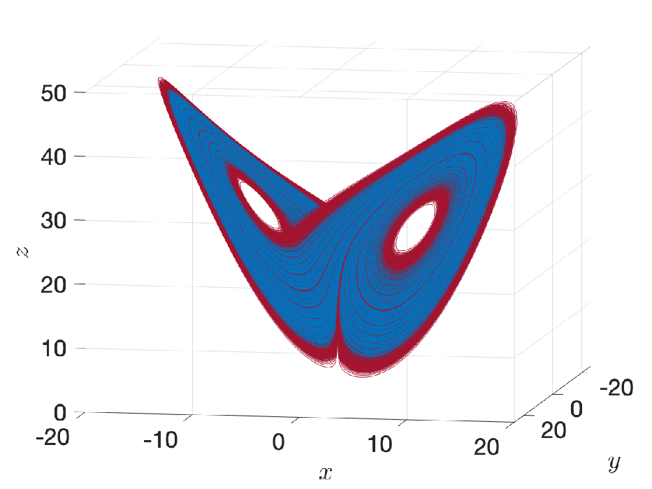
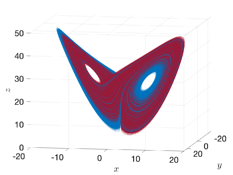
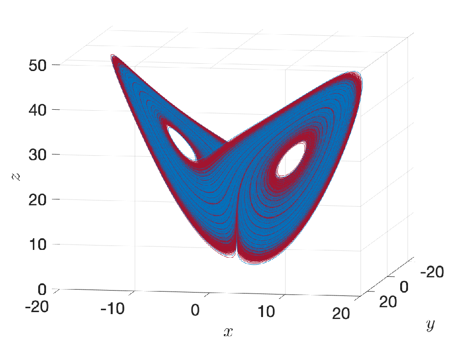
III.4 Relaxation Modes
The red-and-blue representation of the subdominant modes given in Figs. 6a-6c is essentially qualitative because we distinguish the various UPOs only in terms of the sign of their projection on the eigenvectors. We want now to portray the eigenmodes in , in such a way that it is possible to retain quantitative information associated to the evolution of ensembles of trajectories. We proceed as follows. We partition the compact subset of given by the Cartesian product . As mentioned before, this set includes the attractor of the L63 model. We cover this region with cubes with sides having unitary length. The cubes are built having adjacent sides, so that constitutes a partition of . Each UPO and corresponding neighbourhood intersects a certain number of cubes and each cube might contain contributions from different orbits. We now define a quantity (mass) that weights the contribution given by UPOs of different types within each cube. We set a fixed number of points to be represented in the phase space a priori and assign the points to the different UPOs and relative neighbourhood depending on the weight given by the corresponding component of the eigenvector . These points are chosen along the orbits equally spaced in time. We also distinguish between negative and positive contributions, depending on the sign of the component . We finally quantify the mass contained in each cube of the partition by calculating the algebric sum of the points contained in it.
Correspondingly, Fig. 7a describes the invariant measure, while Figs. 7b, 7c, and 7d describe the eigenvectors corresponding to the subdominant eigenvalues , , and , respectively. The eigenvectors , , and are the three slowest modes responsible for the relaxation of an initial probability measure towards the invariant one, the rate of convergence being given by the corresponding eigenvalues. By construction, one can see a good correspondence between the red and blue regions in the panels of Figs. 6 and 7 associated with the same eigenvalue. Indeed, the physical process responsible for the slow decay of anomalies of an ensemble with respect to the invariant measure described in Fig. 7 is indeed the slow mixing occurring in phase space between the regions described by the quasi-invariant sets associated with different bundles of UPOs depicted in Fig. 6. We observe that the smaller the eigenvalue, thus associated to faster decay rate, the finer the geometrical structure associated with the mode. This agrees with our intuition on how diffusion works.


III.5 Remark
The reader might wonder how robust the results presented in Figs. 6a-6c and Figs. 7a-7d with respect to the shadowing criteria defined in Eq. 5, which takes into consideration only tier 1 shadowing UPOs. To assess the robustness of the method, we have repeated our analysis using the looser definition of shadowing described in Sect. II.4 that leads to increased persistence of the co-evolution of the chaotic trajectory and of the shadowing UPOs described in Fig. 3b. The results are presented in the supplementary material. The subdominant eigenvectors change very little as larger values of are considered, whereas, as expected the value of the corresponding eigenvalues get closer and closer to 1, so that slower decay of correlation is found. Clearly, this is the probabilistic counterpart of the results shown in Fig. 3b and supports the idea expected, since allowing for more persistence in the shadowing of the chaotic trajectory results in less frequent transitions and thus slower decay rates.
IV Summary and Conclusion
The theory of UPOs has found extensive applications in the study of low-dimensional chaotic systems, in particular as a mean to calculate dynamical averages through the use of trace formulas Eckhardt and Ott 1994; Franceschini, Giberti, and Zheng 1993; Zoldi 1998. In recent times promising developments have been made regarding its use for understanding the behaviour of higher dimension dynamical systems Kawahara and Kida 2001; Gritsun 2008; Gritsun 2013; Lucarini and Gritsun 2020; Cvitanović 2013; Chandler and Kerswell 2013. Very recently, efforts has been dedicated to better understanding the similarity of chaotic trajectory segments and of locally approximating UPOs in fluid flows Yalniz and Budanur 2020; Krygier, Pughe-Sanford, and Grigoriev 2021. It usually assumed that the low-period UPOs are the most relevant ones for achieving an accurate representation of statistical properties of the system Eckhardt and Ott 1994; Cvitanović 1995; Artuso, Aurell, and Cvitanovic 1990a; Hunt and Ott 1996; Yang, Hunt, and Ott 2000. Nonetheless, even if the trace formulas Cvitanović 1988 seem to suggest the opposite, it is sometimes found that long-period UPOs can be of great importance for computing statistical averages Zoldi and Greenside 1998; Lasagna 2018; Lasagna 2020. Additionally, UPOs have been used as a way to perform coarse-graining: it has been shown that it is possible to approximate accurately the evolution of a fluid flow using a finite-state Markov chain where each state corresponds to the neighborhood of a UPOs Yalniz, Hof, and Budanur 2021. Finally, specific UPOs have been shown to key to separating quasi-invariant sets for the L63 model Froyland and Padberg 2009.
In this work we have attempted to bring together these research lines by performing an accurate analysis of how a long chaotic trajectory of the L63 model with the standard parameter values can be approximated using the complete set of UPOs having symbolic dynamics with period up to 14, numbering 2536 UPOs. The chaotic trajectory can be seen as a continuous process of scattering between the neighbourhood of the various UPOs. At each time step, we rank the UPOs in terms of their distance to reference point, and investigate how the distances and the ranking changes in time. The shadowing of the trajectory involves both proximity and the fact that, as a result of the smoothness of the flow, the reference point of the trajectory and of the considered UPOs co-evolve; indeed we can say that the rectified distance of the co-evolving UPO with the trajectory is of order of magnitude larger than the initial distance between the two. We find that longer UPOs, as a result of their higher number and longer spatial extent, are the most effective in shadowing the orbit of the system. This holds true if we consider a relaxed version of our algorithm, which allow for the rank of the shadowing UPO to fluctuate up to a certain threshold (very good vs. optimal shadowing).
We then investigated a finite-state representation of the dynamics where each state is given by an UPO and its neighbourhood, and the stochastic matrix is defined in a frequentist way by studying the transitions defining the time-dependent shadowing of the chaotic trajectory. Since we are implementing a discretized representation of the transfer operator, the eigenvectors corresponding to the subdominant eigenvalues describe the process of relaxation of ensembles towards the invariant measure. While a similar UPOs-based Markov chain model has been recently proposed by Yalniz, Hof, and Budanur 2021 with the goal of computing averages, to the best of our knowledge, this is the first time this specific discretization is performed with the purpose of analysing the mixing properties of the system. By projecting the UPOs on the 3D space, we find that eigenvectors with finer spatial structures have faster decaying rates. Additionally, building on the fact that UPOs are invariant sets that transport mass across the attractor, the regions of the eigenvectors having the same sign can be thought as approximately defining quasi-invariant sets. Indeed, the patterns defined in this way exhibit qualitative agreement with the structures found in the L63 model by Froyland and Froyland and Padberg in Froyland 2001 and Froyland and Padberg 2009 using the discretization of the transfer operator based on the classical Ulam’s partition. We interpret our findings as follows. The forward trajectory typically undergoes scattering between UPOs belonging to a bundle of UPOs associated with a quasi-invariant set, while, rarely, the scattering process bring the trajectory with close proximity of an UPO belonging to the other bundle, associated with a competing quasi-invariant set.
Clearly, further research is needed in this direction in order to assess differences and similarities between these approaches. Our procedure seems to have a good degree of robustness. It is encouraging to see that if we construct the stochastic matrix using the relaxed definition of the shadowing mentioned above, the eigenvectors corresponding to the subdominant eigenvalues are virtually unchanged, whereas the decay rates become slower, as persistence is enhanced by slowing down the transitions between the competing neighbourhoods.
This work provides further support to the potential of using UPOs for reaching a comprehensive understanding of the properties - averages and correlations - of chaotic dynamical systems. We would like to extend this analysis to higher dimensional system of practical relevance. In particular we would like to extend the work of Lucarini and Gritsun Lucarini and Gritsun 2020 on blocking events, investigating transitions between zonal flow and blocking by applying the methodology developed in this paper. The investigation of this model is of interest both in terms of the physical process of interest - the low-frequency variability of the atmosphere is far from being a settled problem - and in terms of its mathematical properties, as it is characterised by high variability in the number of unstable dimension, thus featuring a serious violation of hyperbolicity.
Appendix A Unstable Periodic Orbits Search
We will review here the classic Newton algorithm Parker and Chua 2012 for detecting UPOs of the ordinary differential equation
| (12) |
where is a compact manifold. This method is particularly appropriate for finding periodic solutions even in high-dimensional systems.
The problem of numerically finding UPOs can be reduced to the solution of the periodicity condition, which corresponds to a system of nonlinear equations with respect to the initial condition of the UPO and its period:
| (13) |
where is the initial condition and is the period of the UPO. Even for simple nonlinear systems this represents a difficult numerical problem. Hence, the choice of the algorithm and initial guess represent an important aspect to be considered. We first rewrite the periodicity condition 13 as follows:
| (14) |
This is a system of nonlinear equations (n is the dimension of the phase space) in unknowns (the vector and the orbit period T). We start with an initial condition (, T). A way to choose it is by calculating a long trajectory and selecting a quasi-recurrence occurring over a period T such that with decided a priori. Let then be and the th approximations for initial condition and period. The aim of the algorithm is to calculate a correction so that we can improve the initial guess in such a way that
| (15) |
We obtain the approximate corrections by expanding
| (16) |
into a Taylor series with respect to and
| (17) |
where is the identity matrix of order . is the tangent linear operator and it is an approximation of the monodromy matrix Cvitanovic et al. 2005. is the derivative of the solution with respect to time evaluated at the final condition . In order to remove the excess in degrees of freedom, we impose the phase condition by requiring the orthogonality of the correction vector to the orbit
| (18) |
In this way we reduce the problem of finding the corrections at step to the solution of a linear system of equations in unknowns
| (19) |
The solution of Eq. 19 gives the next approximations for the UPO initial condition and period. In some cases the Newton method may not give convergence (or the convergence could be very slow) if the initial guess is far from the solution, so that the linear Taylor expansion is not valid or the linear system is degenerate. In this case, one can use a nonlinear expansion in Eq. 17 as well as step relaxation together with line search procedure (see Gritsun 2008 for more details).
We consider quasi-recurrent orbits as initial conditions. We integrate the system for a long time starting from a random initial state; the result is a numerical trajectory consisting of the set of ordered points . We then calculate the quantity and take the minimum, obtained at say . We have a pair of points for which the trajectory starting from passes again near the starting point in time . We can then consider the pairs as initial condition for determining the UPO with the Newton method.
The numerical trajectories have been calculated using the midpoint numerical scheme, with integration time-step of . We choose an output time step and consider a UPO to be detected when with .
Appendix B Quasi invariant sets
We here introduce some key ideas regarding the macroscopic structures and large scale dynamics of the system. When the behaviour of individual trajectory is hard to predict, as it is the case in chaotic systems, the study of the global evolution of densities represents a powerful tool to gain insight into the dynamics. In fact, even if it is not possible to characterise the evolution of a single initial condition, it often happens that we can group the phase space in sets characterised by predictable behaviour. Despite chaotic systems are often transitive, this property can be very weak and it is often the case that the phase space can be decomposed in macroscopic dynamical structure such that the probability of individual trajectories beginning in the subset would leave it in short time is very little. Trajectories tend to stay for a very long time in one of those regions before entering another region. We call these subsets quasi-invariant sets. More precisely, Froyland and Padberg 2009 let be a smooth vector field, generating the dynamical system or flow , be the flow of the autonomous system, preserved by . We say that a subset is almost-invariant over the interval if
| (20) |
Quasi-invariant sets can also be regarded as a valuable tool to study transport and mixing properties of the flow Froyland and Padberg-Gehle 2014, by evolving with minimal dispersion.
Acknowledgements.
The authors have benefitted from scientific exchanges with P. Cvitanović, J. Dorrington, G. Ducci, G. Froyland, C. Nesbitt, M. Santos, N. Zagli, M. Zaks and from the very constructive criticism by two anonymous reviewers. AG was supported by the Moscow Center of Fundamental and Applied Mathematics (Agreement 075-15-2019-1624 with the Ministry of Education and Science of the Russian Federation).VL acknowledges the support received from the EPSRC project EP/T018178/1 and from the EU Horizon 2020 project TiPES (grant no. 820970). CCM has been supported by an EPSRC studentship as part of the Centre for Doctoral Training in Mathematics of Planet Earth (grant number EP/L016613/1). The authors acknowledge the support received from Institutional Sponsorship-International Partnerships-University of Reading EP/W524268/1.Data Availability Statement
The data that support the findings of this study, extra figures, videos, and further details on the methodology can be accessed through the project "Decomposing the Dynamics of the Lorenz 1963 model using Unstable Periodic Orbits: Averages, Transitions, and Quasi-Invariant Sets" at https://tinyurl.com/4z6hh9a3.
References
- Poincaré (1893) H. Poincaré, Les méthodes nouvelles de la mécanique céleste: Méthodes de MM. Newcomb, Glydén, Lindstedt et Bohlin. 1893, Vol. 2 (Gauthier-Villars it fils, 1893).
- Cvitanović (1991) P. Cvitanović, “Periodic orbits as the skeleton of classical and quantum chaos,” Physica D: Nonlinear Phenomena 51, 138–151 (1991).
- Cvitanovic et al. (2005) P. Cvitanovic, R. Artuso, R. Mainieri, G. Tanner, G. Vattay, N. Whelan, and A. Wirzba, “Chaos: classical and quantum,” ChaosBook. org (Niels Bohr Institute, Copenhagen 2005) 69, 25 (2005).
- Grebogi, Ott, and Yorke (1988) C. Grebogi, E. Ott, and J. A. Yorke, “Unstable periodic orbits and the dimensions of multifractal chaotic attractors,” Physical Review A 37, 1711 (1988).
- Eckmann and Ruelle (1985) J.-P. Eckmann and D. Ruelle, “Ergodic theory of chaos and strange attractors,” The theory of chaotic attractors , 273–312 (1985).
- Bowen (1975) R. Bowen, “-limit sets for axiom a diffeomorphisms,” Journal of differential equations 18, 333–339 (1975).
- Gutzwiller (2013) M. C. Gutzwiller, Chaos in classical and quantum mechanics, Vol. 1 (Springer Science & Business Media, 2013).
- Cvitanović (1988) P. Cvitanović, “Invariant measurement of strange sets in terms of cycles,” Physical Review Letters 61, 2729 (1988).
- Ruelle (2004) D. Ruelle, Thermodynamic formalism: the mathematical structure of equilibrium statistical mechanics (Cambridge University Press, 2004).
- Ruelle (1999) D. Ruelle, “Smooth dynamics and new theoretical ideas in nonequilibrium statistical mechanics,” Journal of Statistical Physics 95, 393–468 (1999).
- Katok and Hasselblatt (1997) A. Katok and B. Hasselblatt, Introduction to the modern theory of dynamical systems, 54 (Cambridge university press, 1997).
- Smale et al. (1967) S. Smale et al., “Differentiable dynamical systems,” Bulletin of the American mathematical Society 73, 747–817 (1967).
- Bowen (1972) R. Bowen, “Periodic orbits for hyperbolic flows,” American Journal of Mathematics 94, 1–30 (1972).
- Gallavotti (2014) G. Gallavotti, Nonequilibrium and irreversibility (Springer, 2014).
- Gallavotti (1998) G. Gallavotti, “Chaotic dynamics, fluctuations, nonequilibrium ensembles,” Chaos: An Interdisciplinary Journal of Nonlinear Science 8, 384–392 (1998).
- Gallavotti and Cohen (1995) G. Gallavotti and E. G. D. Cohen, “Dynamical ensembles in nonequilibrium statistical mechanics,” Physical review letters 74, 2694 (1995).
- Eckhardt and Ott (1994) B. Eckhardt and G. Ott, “Periodic orbit analysis of the lorenz attractor,” Zeitschrift für Physik B Condensed Matter 93, 259–266 (1994).
- Cvitanović (1995) P. Cvitanović, “Dynamical averaging in terms of periodic orbits,” Physica D: Nonlinear Phenomena 83, 109–123 (1995).
- Artuso, Aurell, and Cvitanovic (1990a) R. Artuso, E. Aurell, and P. Cvitanovic, “Recycling of strange sets: I. cycle expansions,” Nonlinearity 3, 325 (1990a).
- Hunt and Ott (1996) B. R. Hunt and E. Ott, “Optimal periodic orbits of chaotic systems,” Phys. Rev. Lett. 76, 2254–2257 (1996).
- Yang, Hunt, and Ott (2000) T.-H. Yang, B. R. Hunt, and E. Ott, “Optimal periodic orbits of continuous time chaotic systems,” Phys. Rev. E 62, 1950–1959 (2000).
- Zoldi and Greenside (1998) S. M. Zoldi and H. S. Greenside, “Comment on “optimal periodic orbits of chaotic systems”,” Phys. Rev. Lett. 80, 1790–1790 (1998).
- Lasagna (2018) D. Lasagna, “Sensitivity analysis of chaotic systems using unstable periodic orbits,” SIAM Journal on Applied Dynamical Systems 17, 547–580 (2018).
- Lasagna (2020) D. Lasagna, “Sensitivity of long periodic orbits of chaotic systems,” Physical Review E 102, 052220 (2020).
- Chandler and Kerswell (2013) G. J. Chandler and R. R. Kerswell, “Invariant recurrent solutions embedded in a turbulent two-dimensional kolmogorov flow,” Journal of Fluid Mechanics 722, 554–595 (2013).
- Auerbach et al. (1987) D. Auerbach, P. Cvitanović, J.-P. Eckmann, G. Gunaratne, and I. Procaccia, “Exploring chaotic motion through periodic orbits,” Physical Review Letters 58, 2387 (1987).
- Artuso, Aurell, and Cvitanovic (1990b) R. Artuso, E. Aurell, and P. Cvitanovic, “Recycling of strange sets: Ii. applications,” Nonlinearity 3, 361 (1990b).
- Lorenz (1963) E. N. Lorenz, “Deterministic nonperiodic flow,” Journal of atmospheric sciences 20, 130–141 (1963).
- Lucarini (2009) V. Lucarini, “Evidence of dispersion relations for the nonlinear response of the lorenz 63 system,” Journal of Statistical Physics 134, 381–400 (2009).
- Cvitanović (2013) P. Cvitanović, “Recurrent flows: the clockwork behind turbulence,” Journal of Fluid Mechanics 726, 1–4 (2013).
- Kawahara and Kida (2001) G. Kawahara and S. Kida, “Periodic motion embedded in plane couette turbulence: regeneration cycle and burst,” Journal of Fluid Mechanics 449, 291 (2001).
- Gritsun (2008) A. Gritsun, “Unstable periodic trajectories of a barotropic model of the atmosphere.” Russian Journal of Numerical Analysis and Mathematical Modelling 23 (2008).
- Gritsun (2013) A. Gritsun, “Statistical characteristics, circulation regimes and unstable periodic orbits of a barotropic atmospheric model,” Philosophical Transactions of the Royal Society A: Mathematical, Physical and Engineering Sciences 371, 20120336 (2013).
- Gritsun and Lucarini (2017) A. Gritsun and V. Lucarini, “Fluctuations, response, and resonances in a simple atmospheric model,” Physica D: Nonlinear Phenomena 349, 62–76 (2017).
- Lucarini and Gritsun (2020) V. Lucarini and A. Gritsun, “A new mathematical framework for atmospheric blocking events,” Climate Dynamics 54, 575–598 (2020).
- Faranda, Messori, and Yiou (2017) D. Faranda, G. Messori, and P. Yiou, “Dynamical proxies of north atlantic predictability and extremes,” Scientific Reports 7, 41278 (2017).
- Lai, Nagai, and Grebogi (1997) Y.-C. Lai, Y. Nagai, and C. Grebogi, “Characterization of the natural measure by unstable periodic orbits in chaotic attractors,” Phys. Rev. Lett. 79, 649–652 (1997).
- Yalniz and Budanur (2020) G. Yalniz and N. B. Budanur, “Inferring symbolic dynamics of chaotic flows from persistence,” Chaos: An Interdisciplinary Journal of Nonlinear Science 30, 033109 (2020).
- Krygier, Pughe-Sanford, and Grigoriev (2021) M. C. Krygier, J. L. Pughe-Sanford, and R. O. Grigoriev, “Exact coherent structures and shadowing in turbulent taylor–couette flow,” Journal of Fluid Mechanics 923, A7 (2021).
- Ulam (2004) S. M. Ulam, Problems in modern mathematics (Courier Corporation, 2004).
- Yalniz, Hof, and Budanur (2021) G. Yalniz, B. Hof, and N. B. Budanur, “Coarse graining the state space of a turbulent flow using periodic orbits,” Phys. Rev. Lett. 126, 244502 (2021).
- Froyland (2005) G. Froyland, “Statistically optimal almost-invariant sets,” Physica D: Nonlinear Phenomena 200, 205–219 (2005).
- (43) The supplementary material can be accessed at https://tinyurl.com/4z6hh9a3.
- Pikovsky and Politi (2016) A. Pikovsky and A. Politi, Lyapunov exponents: a tool to explore complex dynamics (Cambridge University Press, 2016).
- Ott (2002) E. Ott, Chaos in dynamical systems (Cambridge university press, 2002).
- Tucker (1999) W. Tucker, “The lorenz attractor exists,” Comptes Rendus de l’Académie des Sciences-Series I-Mathematics 328, 1197–1202 (1999).
- Galias and Zgliczyński (1998) Z. Galias and P. Zgliczyński, “Computer assisted proof of chaos in the lorenz equations,” Physica D: Nonlinear Phenomena 115, 165–188 (1998).
- Tucker (2002) W. Tucker, “A rigorous ode solver and smale’s 14th problem,” Foundations of Computational Mathematics 2, 53–117 (2002).
- Franceschini, Giberti, and Zheng (1993) V. Franceschini, C. Giberti, and Z. Zheng, “Characterization of the lorentz attractor by unstable periodic orbits,” Nonlinearity 6, 251 (1993).
- Zoldi (1998) S. M. Zoldi, “Unstable periodic orbit analysis of histograms of chaotic time series,” Physical review letters 81, 3375 (1998).
- Saiki and Yamada (2010) Y. Saiki and M. Yamada, “Reply to “comment on ‘time-averaged properties of unstable periodic orbits and chaotic orbits in ordinary differential equation systems’”,” Physical Review E 81, 018202 (2010).
- Saiki and Yamada (2009) Y. Saiki and M. Yamada, “Time-averaged properties of unstable periodic orbits and chaotic orbits in ordinary differential equation systems,” Physical Review E 79, 015201 (2009).
- Zaks and Goldobin (2010) M. A. Zaks and D. S. Goldobin, “Comment on “time-averaged properties of unstable periodic orbits and chaotic orbits in ordinary differential equation systems”,” Physical Review E 81, 018201 (2010).
- Saiki (2007) Y. Saiki, “Numerical detection of unstable periodic orbits in continuous-time dynamical systems with chaotic behaviors,” Nonlinear Processes in Geophysics 14, 615–620 (2007).
- Barrio, Dena, and Tucker (2015) R. Barrio, A. Dena, and W. Tucker, “A database of rigorous and high-precision periodic orbits of the lorenz model,” Computer Physics Communications 194, 76–83 (2015).
- Viswanath (2003) D. Viswanath, “Symbolic dynamics and periodic orbits of the lorenz attractor,” Nonlinearity 16, 1035 (2003).
- Galias and Tucker (2009) Z. Galias and W. Tucker, “Symbolic dynamics based method for rigorous study of the existence of short cycles for chaotic systems,” in 2009 IEEE International Symposium on Circuits and Systems (IEEE, 2009) pp. 1907–1910.
- Bowen (1970) R. Bowen, “Topological entropy and axiom a,” in Proc. Sympos. Pure Math, Vol. 14 (1970) pp. 23–41.
- Palmer (1993) T. Palmer, “Extended-range atmospheric prediction and the lorenz model,” Bulletin of the American Meteorological Society 74, 49–65 (1993).
- Sparrow (1982) C. Sparrow, “The lorenz equations,” Edited by Arun V. Holden , 111 (1982).
- Baladi (2000) V. Baladi, Positive transfer operators and decay of correlations, Vol. 16 (World scientific, 2000).
- Froyland (2001) G. Froyland, “Extracting dynamical behavior via markov models,” in Nonlinear dynamics and statistics (Springer, 2001) pp. 281–321.
- Froyland (1998) G. Froyland, “Approximating physical invariant measures of mixing dynamical systems in higher dimensions,” Nonlinear Analysis: Theory, Methods and Applications 32, 831–860 (1998).
- Lucarini (2016) V. Lucarini, “Response operators for markov processes in a finite state space: Radius of convergence and link to the response theory for axiom a systems,” Journal of Statistical Physics 162, 312–333 (2016).
- Santos Gutiérrez and Lucarini (2020) M. Santos Gutiérrez and V. Lucarini, “Response and sensitivity using markov chains,” Journal of Statistical Physics 179, 1572–1593 (2020).
- Dellnitz and Junge (1999) M. Dellnitz and O. Junge, “On the approximation of complicated dynamical behavior,” SIAM Journal on Numerical Analysis 36, 491–515 (1999).
- Dellnitz and Junge (1997) M. Dellnitz and O. Junge, “Almost invariant sets in chua’s circuit,” International Journal of Bifurcation and Chaos 7, 2475–2485 (1997).
- Froyland (2008) G. Froyland, “Unwrapping eigenfunctions to discover the geometry of almost-invariant sets in hyperbolic maps,” Physica D: Nonlinear Phenomena 237, 840–853 (2008).
- Froyland and Dellnitz (2003) G. Froyland and M. Dellnitz, “Detecting and locating near-optimal almost-invariant sets and cycles,” SIAM Journal on Scientific Computing 24, 1839–1863 (2003).
- Froyland and Padberg (2009) G. Froyland and K. Padberg, “Almost-invariant sets and invariant manifolds—connecting probabilistic and geometric descriptions of coherent structures in flows,” Physica D: Nonlinear Phenomena 238, 1507–1523 (2009).
- Parker and Chua (2012) T. S. Parker and L. Chua, “Practical numerical algorithms for chaotic systems,” (2012).
- Froyland and Padberg-Gehle (2014) G. Froyland and K. Padberg-Gehle, “Almost-invariant and finite-time coherent sets: directionality, duration, and diffusion,” in Ergodic Theory, Open Dynamics, and Coherent Structures (Springer, 2014) pp. 171–216.