Renormalization group improvement of the effective potential in a dimensional Gross-Neveu model
Abstract
In this work, we investigate the consequences of the Renormalization Group Equation (RGE) in the determination of the effective potential and the study of Dynamical Symmetry Breaking (DSB) in an Gross-Neveu (GN) model with fermions fields in dimensional space-time, which can be applied as a model to describe certain properties of the polyacetylene. The classical Lagrangian of the model is scale invariant, but radiative corrections to the effective potential can lead to dimensional transmutation, when a dimensionless parameter (coupling constant) of the classical Lagrangian is exchanged for a dimensionful one, a dynamically generated mass for the fermion fields. For the model we are considering, perturbative calculations of the effective potential and renormalization group functions up to three loops are available, but we use the RGE and the leading logs approximation to calculate an improved effective potential, including contributions up to six loops orders. We then perform a systematic study of the general aspects of DSB in the GN model with finite N, comparing the results we obtain with the ones derived from the original unimproved effective potential we started with.
I Introduction
In quantum field theory Dynamical Symmetry Breaking (DSB) is a key mechanism that has applications in particle physics and condensed matter systems (Gross; Chodos1994; Campbell1982), where quantum corrections are entirely responsible for the appearance of nontrivial minima of the effective potential. In the case of particle physics, for example, we have a Higgs mechanism playing a fundamental role in the Standard Model: in this case, the symmetry breaking requires a mass parameter in the tree-level Lagrangian, but Coleman and Weinberg (CW) demonstrated (Coleman1973) that spontaneous symmetry breaking may occur due to radiative corrections even when this mass parameter is absent from the Lagrangian (which is, therefore, scale invariant). For the study of the CW mechanism, we need to calculate the effective potential, a powerful tool to explore many aspects of the low-energy sector of a quantum field theory. In many cases, the one-loop approximation is good enough, but it can be improved it, by adding higher order contributions in the loop expansion. A standard tool for improving a perturbative calculation performed up to some loop level is the Renormalization Group Equation (RGE) which, together with a reorganization of the perturbative results in terms of leading logs, have been shown to be very effective (AHMADY2003221; PhysRevD.72.037902; Souza2020; Quinto2016; Dias2014; CHISHTIE2007). We refer the reader to section 3 in (Quinto2016) for a short review of the method, and (Elias2003; Chishtie2006; Chishtie2011; Steele2013) for some of the interesting results that have been reported with the use of the RG improvement.
The Gross-Neveu (GN) model with fermions has great relevance in the study of the polyacetylene, , which is a polymer with conductive properties which are acquired through doping (Chiang1977). Polyacetylene is a straight chain that can have two forms, trans and cis. The trans form (trans-polyacetylene), which is the most stable, has a doubly degenerate ground state. These circumstances allow the existence of topological excitations, which entails a great phenomenological richness in this type of models. In (Campbell1982; Takayama1980) it was shown that in the continuous limit, and in the approximation where the dynamical vibration of lattice (phonons) is ignored, the metal-insulator transition in the polyacetylene can be described by the GN model in . In addition, the polyacetylene exhibits some remarkable effects, such as the Peierls mechanism (Horovitz1993), which is the generation of an energy gap for electrons through the coupling with phonons. This mechanism is analogous to the Yukawa interaction in the Standard Model.
The GN model can be seen as an effective low energy theory for the polyacetylene. This was shown by the Takayama-Lin-Liu-Maki (TLM) model (Takayama1980), where the effective low-energy theories of the Su-Schrieffer-Heeger (SSH) model (Su1979) are described by a theory of four fermions fields in dimensions. In this model the behavior of the energy band (gap) is described as,
| (1) |
where is the width of the energy band, is the Fermi velocity, is the coupling constant between the electron and phonons. If the adiabatic approximation is used in the TLM model, then it can be related to the GN model, and therefore, we can find an expression analogous to Eq. (1), which is related to the mass obtained in GN by symmetry breaking,
| (2) |
being a constant scalar field and a renormalization scale, which is not a physical parameter, and therefore the only quantity that is measured is the mass, . On the other hand, if we compare this with its analog, Eq. (2), and are parameters measured in . Now comparing (1) and (2) we can observe a relationship between the coupling constants,
| (3) |
where we have replaced , which is the relevant value for the description of the polyacetylene.
Our goal here is to study, via radiative corrections, the generation of mass by DSB. In this case the mass will be obtained by
| (4) |
where is the renormalization scale introduced in our model by regularization, and is the effective potential which is a function of the (classical) scalar field .
In this paper, we considered the three loops calculation of renormalization group functions and effective potential for the dimensional GN model with finite (that is to say, without recourse to the expansion) that have been described in (Luperini1991). The RGE is then used to improve this calculation, incorporating terms that originate from higher loop orders (up to six). Then, we study the DSB properties of the model using the unimproved (directly obtained by perturbative calculations) and RGE improved effective potentials, and we observe that the improvement of the effective potential leads to relevant differences in comparison with the unimproved one found in the literature.
There have been many studies of the GN model in the literature, usually considering the expansion. In this regard, Ref. (Blaizot:2002nh) presents a nice review of leading and sub-leading orders in this expansion, at finite temperature. The phase diagram for the model has been first established in Ref. (Wolff:1985av), and recently revised by lattice computations (Pannullo:2019bfn; Pannullo:2019prx; Lenz:2020bxk; Lenz:2020cuv). Another recent study of this phase diagram, using mean-field techniques, is presented in (Stoll:2021ori). Finally, studies using the functional renormalization group have also been reported (Stoll:2021ori). Our approach is complementary, for not resorting to the expansion, thus being particularly adequate for models with small ; on the other hand, it is inherently perturbative. It is also interesting to notice that we work at zero temperature and chemical potential, so we investigate a single point in the phase diagram that was discussed in the above-mentioned works. But, at this single point, we are able to perform calculations analytically. Generalizations for finite temperature and chemical potential are possible, but not trivial, and are left for future works.
This paper is organized as follows: in section. II we present our model with the renormalization group functions and unimproved effective potential found in the literature. In section III we calculate the improvement of effective potential using the standard approach of RGE, and section IV is devoted to study DSB in our model. In section V we present our conclusions and future perspectives.
II Renormalization group functions and unimproved effective potential for Gross-Neveu model
We start with the Euclidean formulation of the massless dimensional GN model studied by Luperini and Rossi (Luperini1991) whose Lagrangian with fermions fields and symmetry is,
| (5) |
This model has a discrete invariance , whose spontaneous breakdown leads to a nonzero vacuum expectation value and thus to a dynamical mass generation (Gross). Also, the model is known to be asymptotically free in two dimensions, and can be extended to,
| (6) |
where is the scalar field, is the fermion field, and are dimensionless coupling constants that appear with the introduction of the auxiliary field , which carries the same quantum numbers as , i.e. . The Lagrangians and are equivalent both at classical level (using the equations of motion for in (6) to obtain (5)) as well as at the quantum level, since a gaussian integration over in the partition function calculated from (6) leads to the same partition function derived by (5).
The renormalization group functions and were calculated for this model up to three loop order (see the Ref. (Luperini1991) for more details), and we quote the result,
| (7) |
where
| (8a) | ||||
| (8b) | ||||
| (8c) | ||||
| (9) |
where
| (10a) | ||||
| (10b) | ||||
| (10c) | ||||
| (11) |
where
| (12a) | ||||
| (12b) | ||||
| (12c) |
and
| (13) |
with
| (14a) | ||||
| (14b) | ||||
In the previous equations, the superscript mean the global power of coupling constant in each term. This notation will be usefull to organize the terms for the calculation of the improved version of the effective potential, in the next section.
The effective potential was also calculated up to three loops, in the minimal subtraction (MS) scheme, as follows,
| (15) |
with
| (16) |
where
| (17) |
being the mass scale that is introduced to keep the dimensions of the relevant quantities unchanged, and
| (18) |
where is known as Apéri constant.
III Improvement of effective potential for the GN model
In this section we compute the improvement of effective potential of the model defined by the Lagrangian (6). We start with
| (19) |
where is a function that remains to be determined. On dimensional grounds, we can assume the following Ansatz,
| (20) |
where is given by Eq. (17), and the coefficients , , and are functions only of the (dimensionless) coupling constants. The main idea behind the method is the observation that the coefficients in (20) are not all independent, since changes in must be compensated for by changes in the other parameters, according to the renormalization group. This is the same as saying that the effective potential has to satisfy a RGE. Following the procedure in (Quinto2016; AHMADY2003221; CHISHTIE2007), and using the conventions given in (Luperini1991) and quoted in the last section, we can write the RGE for in the form
| (21) |
where the renormalization group functions are defined by equations (7), (9), (11) and (13).
One should note, at this point, that these functions were computed (Luperini1991) in the MS scheme. In principle, they should be adapted to a different scheme for our applications – however, as discussed in (Quinto2016), this is not necessary when UV divergences appear at second or higher loop level, as it is the present case. Therefore, this issue does not have to be dealt with and, for our purposes, we can directly apply the renormalization group equations obtained in (Luperini1991) for the RGE improvement.
If we use the Ansatz in Eq. (20) together with Eq. (21), it is possible to calculate recursively, order by order in the coupling constants, the functions , , and . In particular, is fixed by the tree-level effective potential, Eq. (18), in the form
| (22) |
where with are known functions, and again the superscript represents the global power of coupling constants in each term. Following the same pattern, we want to calculate the remaining functions order by order in coupling constants, so we also write,
| (23) | ||||
| (24) | ||||
| (25) |
Terms of in the RGE correspond to the function in the Ansatz (20). These can be calculated from our knowledge of and the renormalization group functions. To do that, we substitute (20) into (21) and separate the terms proportional to , obtaining the following expression,
| (26) |
Substituting (22) and (23), together with the renormalization group functions, Eqs. (7), (9), (11) and (13), into (26) leads us to the following expression,
| (27) | ||||
and from the previous equation, we can obtain,
| (28a) | ||||
| (28b) | ||||
| (28c) | ||||
| (28d) | ||||
| (28e) |
| (28f) |
| (28g) |
For the purpose of this paper, we will only consider terms up to sixth order in the coupling constants because we only know the function up to four order.
Terms of in the RGE will lead to the calculation of the ’s in (24) from the knowledge we already have from the perturbative calculations, as well as the ’s that we just obtained. Repeating the same procedure as before, we find the following results,
| (29a) | ||||
| (29b) | ||||
| (29c) | ||||
| (29d) |
| (29e) |
| (29f) |
Going to in the RGE, we can find all the ´s in (25), and the result is,
| (30a) | ||||
| (30b) | ||||
| (30c) | ||||
| (30d) |
| (30e) |
Finally, with the values of and that have been obtained, we obtain , which we call the improved effective potential, since it contains higher-orders (in the coupling constants) terms that were obtained from the RGE, and beyond what can be obtained by direct loop calculation, as presented in Sec. II. Notice that it is possible to obtain the unimproved version of the effective potential, , that was calculated up to three loop order in (Luperini1991) by setting , and . This is a proof of the consistency of our calculations.
IV Dynamical symmetric breaking
We start this section analyzing the behavior of the DSB for the unimproved and improved versions of the effective potential, Eq. (15). First, one has to recognize that the effective potentials that we computed actually correspond to the regularized effective potential, and we still need to fix a finite renormalization constant that is introduced via
| (31) |
where can be fixed with the Coleman-Weinberg (CW) (Coleman1973) condition,
| (32) |
The second step is to enforce that has a minimum at . This is done imposing the condition,
| (33) |
together with
| (34) |
where is the mass generated by radiative corrections for the scalar field. It is interesting to notice that, here, this last condition (34) is actually equivalent to the CW condition, that is to say, Eq. (34) is automatically satisfied once (32) is enforced. The same does not happen in other models that were studied within this approach, such as (Elias2003; Dias2010; Quinto2016), where Eq. (34) provides an additional selection rule to be considered when looking into solutions for Eq. (33).
From a computational point of view, since we want to study the general properties of the DSB mechanism in this model for a wide range of the values of its coupling constants, we will use Eq. (33) to fix the value of the constant as a function of and , which will remain as free parameters. Also, at this point, the rescaling and suggested in (Luperini1991) was implemented. Upon explicit calculation, Eq. (33) turns out to be a polynomial equation in , and among its solutions we look for those which are real and positive, and which lie in the perturbative regime, .
To analyze the DSB in our model both for the unimproved and improved cases, we created a program in Mathematica© to systematically apply the previous steps for arbitrary values of the free parameters. In other words: for any reasonable value of and , we apply the CW condition, Eq. (32), to fix the renormalization constant , then we use Eq. (33) to find solutions of in terms of and , from which we separate the physical solutions that are real and positive, and also satisfy to ensure we are within the perturbative regime. Any solution with is discarded as nonphysical, since our approach is inherently perturbative. This procedure is applied both for the unimproved and improved regularized effective potentials, for the sake of comparing both cases, and we denote as the value of the coupling constant obtained with the improved potential, and with the unimproved one.
As a first step, the parameters space in which the DSB is operational was found by scanning the whole parameter space determined by and , and obtaining a region plot showing where the DSB occurs (i.e., the region where the previously explained procedure yields consistent minima away from the origin). These plots are presented in the figure 1, both for the unimproved (figure 1a) and improved (figure 1b) cases. As we can see, the parameter space for which the DSB is possible in the improved case is much smaller than the unimproved one, which is consistent with previous results in this type of studies, for example in three and four dimensional space-time models (Quinto2016; Dias2014).


We also observed the existence of more than one possible solution for and for a given value of and . For this, the coupling constants for both cases were plotted as a function of in the interval of for different fixed values of , as shown in figure 2.


It is interesting to note that for (figure 2a), there is a single solution for in both cases. Also, we note that there is a very small difference between and for an interval of values of . However, we can consider an example where it is possible to observe the behavior between the minimum of improved and unimproved effective potentials, for the values of and respectively, corresponding to and , as we shown in the figure 3.
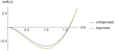
On the other hand, if we analyze the cases , , and , which are shown in figures 2b to 2d, we observe that they present more than one value for , while continues with a single value. We note that a set of values of only appear for small values of and these tend to decrease as increases. To observe the effects of these values on the minimum of potentials, we consider an example where , , , and , as we shown in figure 4. We observe that there is not much difference in the minimum of the effective potential for the values of and considered in this example. Finally, the plot in figure 4 also exemplifies the fact that, for several of the solutions defined by and , the point is actual a meta-stable local minima, and not the global minima, which actually appears for .

It is interesting to note the deep differences in the general properties of the DSB mechanism, and quantitative aspects of the mechanism, in the case of the improved effective potential. We also point out that our results are in general compatible with the results obtained in three and four dimensional space-time models, where the improved effective potential was also calculated from the RGE, in the approximation of leading logarithms (Dias2010; Quinto2016; Dias2014; Souza2020; PhysRevD.72.037902; CHISHTIE2007).
We close this section by pointing out the fact that common artifacts of the perturbative calculation of the effective potential are non-convexity and even instabilities (i.e., the potential not being bounded from below). One notable case of this last problem is the so-called conformal limit of the Standard Model, where the inclusion of the top quark contribution to the one loop perturbative effective potential lead to an unstable potential, a problem that was solved by summing up the leading logs corrections using the RGE (Elias2003). Additional improvements of this idea were further developed, and actually led to a calculation of the Higgs mass of , not far from the experimental value of (Steele2013). We can also quote (Meissner:2006zh; Meissner:2008uw) for showing how an improved calculation of the effective potential may cure these ailments.
V Conclusions
In this paper we have studied the behavior of the unimproved and improved effective potential in a massless dimensional Gross-Neveu model with fermions fields. We have observed that the improvement of the effective potential, which we calculated up to the sixth power of the coupling constants, leads to different results in comparison with the unimproved case. As a general rule, the use of the RGE allows us to obtain higher order corrections to the effective potential, based on the knowledge of the renormalization group functions calculated up to some loop level (three in the case we considered here (Luperini1991)), and this could lead to a better understanding of the DSB mechanism.
We notice that the improvement that we have performed in this work has not been able to fully avoid such problems of the perturbative effective potential. We can see in Fig. 4 one of the improved potentials failing to be convex in the region between two local minima. These potentials might also become unstable for larger values of . We believe this comes from the fact that we were able to sum up only contributions up to six loop order in the . A different summation scheme, closer to the one adopted in (Elias2003; Dias2010), might allow for summing up infinite sub-series of higher loop order contributions to , and that would probably eliminate at least some of these problems. This is one topic we want to discuss in a future work.
Another interesting perspective is to incorporate a term associated with the chemical potential: usually this appears as a mass parameter associated with fermions, and it was not considered in the model studied here, since the RGE improvement is simpler when the starting Lagrangian is scale invariant. It has been reported in the literature that the chemical potential is a key ingredient in the study of the polyacetylene properties, corresponding for example to the doping concentration, as discussed in (Chodos1994; Caldas; Caldas2009; Caldas2009a; Kneur2007) up to one loop order. Therefore, the idea would be to observe the behavior of the effective potential when it has an explicit dependence on the chemical potential at higher loop orders. This problem would involve a multi-scale approach to the RGE improvement, as discussed, for example, in (Ford:1996hd; Chataignier:2018aud). The presence of a dimensional constant in the starting Lagrangian leads to the appearance of two independent logarithms in the perturbative expression for the effective potential since there would be, in general, contributions involving also , with the fermion mass, related to the chemical potential. That is another topic we intent to investigate further.
Acknowledgements.
The authors would like to thank André Lehum for his comments about the manuscript, as well as the referee that provided very insightful comments that helped us to improve our paper. This work was partially supported by Fondo Nacional de Financiamiento para la Ciencia, la Tecnología y la Innovación "Francisco José de Caldas", Minciencias Grand No. 848-2019 (AGQ) and by Conselho Nacional de Desenvolvimento Científico e Tecnológico (CNPq), grant 305967/2020-7 (AFF).References
- [1] David J. Gross and Andre Neveu. Dynamical symmetry breaking in asymptotically free field theories. Physical Review D, 10:3235–3253, 1974.
- [2] Alan Chodos and Hisakazu Minakata. The gross-neveu model as an effective theory for polyacetylene. Phys. Lett. A, 191:39, 1994.
- [3] D. K. Campbell and A. R. Bishop. Soliton excitations in polyacetylene and relativistic field theory models. Nuclear Physics B 200, pages 297–328, 1982.
- [4] Coleman Sidney and Weinberg Erick. Radiative corrections as the origin of spontaneous symmetry breaking. Phys. Rev. D, 7:1888–1910, Mar 1973.
- [5] M.R. Ahmady, V. Elias, D.G.C. McKeon, A. Squires, and T.G. Steele. Renormalization-group improvement of effective actions beyond summation of leading logarithms. Nuclear Physics B, 655(3):221–249, 2003.
- [6] V. Elias, R. B. Mann, D. G. C. McKeon, and T. G. Steele. Higher order stability of a radiatively induced 220 gev higgs mass. Phys. Rev. D, 72(3):037902, Aug 2005.
- [7] Huan Souza, L. Ibiapina Bevilaqua, and A. C. Lehum. Renormalization group improvement of the effective potential in six dimensions. Phys. Rev. D, 102(4):045004, 2020.
- [8] A.G. Quinto, A.F. Ferrari, and A.C. Lehum. Renormalization group improvement and dynamical breaking of symmetry in a supersymmetric chern-simons-matter model. Nuclear Physics B, 907:664–677, 2016.
- [9] A.G. Dias, J.D. Gomez, A.A. Natale, A.G. Quinto, and A.F. Ferrari. Non-perturbative fixed points and renormalization group improved effective potential. Physics Letters B, 739:8–12, 2014.
- [10] F. A. CHISHTIE, V. ELIAS, R. B. MANN, D. G. C. MCKEON, and T. G. STEELE. On the standard approach to renormalization group improvement. International Journal of Modern Physics E, 16(06):1681–1685, 2007.
- [11] V. Elias, R. B. Mann, D. G. C. McKeon, and T. G. Steele. Radiative electroweak symmetry breaking revisited. Phys. Rev. Lett., 91:251601, Dec 2003.
- [12] F. A. Chishtie, V. Elias, R. B. Mann, D. G. C. McKeon, and T. G. Steele. Stability of subsequent-to-leading-logarithm corrections to the effective potential for radiative electroweak symmetry breaking. 743:104–132.
- [13] F. A. Chishtie, T. Hanif, J. Jia, R. B. Mann, D. G. C. McKeon, T. N. Sherry, and T. G. Steele. Can the renormalization group improved effective potential be used to estimate the higgs mass in the conformal limit of the standard model? Phys. Rev. D, 83:105009, May 2011.
- [14] T. G. Steele and Zhi-Wei Wang. Is radiative electroweak symmetry breaking consistent with a 125 gev higgs mass? Phys. Rev. Lett., 110:151601, Apr 2013.
- [15] C. K. Chiang, C. R. Fincher, Y. W. Park, A. J. Heeger, H. Shirakawa, E. J. Louis, S. C. Gau, and Alan G. MacDiarmid. Electrical conductivity in doped polyacetylene. Phys. Rev. Lett., 39:1098–1101, Oct 1977.
- [16] Hajime Takayama, Y. R. Lin-Liu, and Kazumi Maki. Continuum model for solitons in polyacetylene. Phys. Rev. B, 21:2388–2393, Mar 1980.
- [17] B. Horovitz. Infrared activity of peierls systems and application to polyacetylene. Solid State Communications, 88:983–988, 1993.
- [18] W. P. Su, J. R. Schrieffer, and A. J. Heeger. Solitons in polyacetylene. Phys. Rev. Lett., 42:1698–1701, Jun 1979.
- [19] Cristina Luperini and Paolo Rossi. Three loop beta function(s) and effective potential in the gross-neveu model. Annals Phys., 212:371–401, 1991.
- [20] Jean-Paul Blaizot, Ramon Mendez-Galain, and Nicolas Wschebor. The Gross-Neveu model at finite temperature at next to leading order in the 1 / N expansion. Annals Phys., 307:209–271, 2003.
- [21] U. Wolff. THE PHASE DIAGRAM OF THE INFINITE N GROSS-NEVEU MODEL AT FINITE TEMPERATURE AND CHEMICAL POTENTIAL. Phys. Lett. B, 157:303–308, 1985.
- [22] Laurin Pannullo, Julian Lenz, Marc Wagner, Björn Wellegehausen, and Andreas Wipf. Inhomogeneous phases in the 1+1 dimensional Gross-Neveu model at finite number of fermion flavors. Acta Phys. Polon. Supp., 13:127, 2020.
- [23] Laurin Pannullo, Julian Lenz, Marc Wagner, Björn Wellegehausen, and Andreas Wipf. Lattice investigation of the phase diagram of the 1+1 dimensional Gross-Neveu model at finite number of fermion flavors. PoS, LATTICE2019:063, 2019.
- [24] Julian Lenz, Laurin Pannullo, Marc Wagner, Björn Wellegehausen, and Andreas Wipf. Inhomogeneous phases in the Gross-Neveu model in 1+1 dimensions at finite number of flavors. Phys. Rev. D, 101(9):094512, 2020.
- [25] Julian J. Lenz, Laurin Pannullo, Marc Wagner, Björn H. Wellegehausen, and Andreas Wipf. Baryons in the Gross-Neveu model in 1+1 dimensions at finite number of flavors. Phys. Rev. D, 102(11):114501, 2020.
- [26] Jonas Stoll, Niklas Zorbach, Adrian Koenigstein, Martin J. Steil, and Stefan Rechenberger. Bosonic fluctuations in the -dimensional Gross-Neveu(-Yukawa) model at varying and and finite . 8 2021.
- [27] A. G. Dias and A. F. Ferrari. Renormalization group and conformal symmetry breaking in the chern-simons theory coupled to matter. Phys. Rev. D, 82:085006, Oct 2010.
- [28] Krzysztof A. Meissner and Hermann Nicolai. Conformal Symmetry and the Standard Model. Phys. Lett. B, 648:312–317, 2007.
- [29] Krzysztof A. Meissner and Hermann Nicolai. Renormalization Group and Effective Potential in Classically Conformal Theories. Acta Phys. Polon. B, 40:2737–2752, 2009.
- [30] Heron Caldas, Jean-Loïc Kneur, Marcus Benghi Pinto, and Rudnei O. Ramos. Critical dopant concentration in polyacetylene and phase diagram from a continuous four-fermi model. Physical Review B 77, 205109, 2008.
- [31] Heron Caldas. Asymmetrically doped one-dimensional trans-polymers. Physica B, 404:3159–3162, 2009.
- [32] Heron Caldas. Asymmetrically doped polyacetylene. Nuclear Physics B, 807:651–658, 2009.
- [33] Jean-Loïc Kneur, Marcus Benghi Pinto, and Rudnei O. Ramos. The 2d gross-neveu model at finite temperature and density with finite n corrections. Brazilian Journal of Physics, 37(1b):258–264, 2007.
- [34] C. Ford and C. Wiesendanger. A Multiscale subtraction scheme and partial renormalization group equations in the O(N) symmetric phi**4 theory. Phys. Rev. D, 55:2202–2217, 1997.
- [35] Leonardo Chataignier, Tomislav Prokopec, Michael G. Schmidt, and Bogumila Swiezewska. Single-scale Renormalisation Group Improvement of Multi-scale Effective Potentials. JHEP, 03:014, 2018.