Power-Law $f(R)$ Gravity Corrected Canonical Scalar Field Inflation

After the primordial quantum epoch, the Universe is believed to have inflated in an abrupt way, during an era which is known as the inflationary era. At the beginning of the inflationary era, the Universe was hot, described by a four dimensional spacetime metric and was more or less in a classical state, with possibly only remnants of the full high energy quantum theory making their presence in the effective inflationary Lagrangian. To date, the most well-known description of inflation is that of a scalar field, the inflaton, which controls the inflationary and early post-inflationary era inflation1; inflation2; inflation3; inflation4. The inflationary scenario solves quite prominent problems of the standard Big Bang scenario, such as the flatness problem and the horizon problem, and several models of scalar field inflation are robust towards the constraints imposed by the latest Planck data Akrami:2018odb. Nevertheless, it is not certain if inflation even occurred, since a direct evidence of the inflationary era would be provided by the observation of $B$-modes (curl) in the Cosmic-Microwave-Background radiation Kamionkowski:2015yta. There are appealing alternative scenarios that may also describe the primordial epoch in a successful way, such as the bouncing cosmology scenarios Brandenberger:2012zb; Brandenberger:2016vhg; Battefeld:2014uga; Novello:2008ra; Cai:2014bea; deHaro:2015wda; Lehners:2011kr; Lehners:2008vx; Cheung:2016wik; Cai:2016hea; Odintsov:2020vjb, and in some cases a dark energy era might be combined with a primordial bounce Odintsov:2020vjb, however all these scenarios, including the inflationary scenario, are for the moment candidate proposals for the primordial epoch of our Universe, and only constraints can be imposed on them.

Scalar field inflation strongly relies on the existence of a primordial scalar field, the inflation, which effectively controls the dynamical evolution of the Universe. However, to date, only the only scalar field that has ever been observed is the Higgs scalar Aad:2012tfa, thus it is compelling to explain how the inflation plays some fundamental role in the high energy physics, and answer the question whether the inflaton is directly related to the Higgs particle or even if the Higgs particle is the inflaton itself. Apart from this, a vital question that should be answered in a concrete way is the effective Lagrangian of inflation itself. Since at the beginning of inflation, the Universe emerged classical from a quantum epoch, it is possible that the quantum epoch left its imprints in the classical effective inflationary Lagrangian. Several scenarios that predict corrections to the canonical scalar field Lagrangian exist in the literature, such as the Einstein-Gauss-Bonnet corrections Hwang:2005hb; Nojiri:2006je; Cognola:2006sp; Nojiri:2005vv; Nojiri:2005jg; Satoh:2007gn; Bamba:2014zoa; Yi:2018gse; Guo:2009uk; Guo:2010jr; Jiang:2013gza; Kanti:2015pda; vandeBruck:2017voa; Kanti:1998jd; Pozdeeva:2020apf; Fomin:2020hfh; DeLaurentis:2015fea; Chervon:2019sey; Nozari:2017rta; Odintsov:2018zhw; Kawai:1998ab; Yi:2018dhl; vandeBruck:2016xvt; Kleihaus:2019rbg; Bakopoulos:2019tvc; Maeda:2011zn; Bakopoulos:2020dfg; Ai:2020peo; Odintsov:2019clh; Oikonomou:2020oil; Odintsov:2020xji; Oikonomou:2020sij; Odintsov:2020zkl; Odintsov:2020sqy; Odintsov:2020mkz; Easther:1996yd; Antoniadis:1993jc; Antoniadis:1990uu; Kanti:1995vq; Kanti:1997br, which are also string theory originating. Another possibility is that at high curvatures, higher order curvature terms may eventually be present in the effective inflationary Lagrangian and these terms can play a dominant role in the inflationary dynamics of simple scalar field inflation. In this line of research, in this paper we shall assume that power-law $f(R)$ gravity terms are present in the effective inflationary Lagrangian of a canonical scalar field, and we shall examine the dynamical evolution of the scalar field in the presence of these power-law $f(R)$ gravity terms of the form $\sim R^{n}$. The $R^{n}$ term will dominate during inflation over the Einstein-Hilbert term $\sim R$, and consequently, the dynamical evolution of the canonical scalar field will be affected in a crucial way. We shall assume that the slow-roll conditions holds true and eventually the whole canonical scalar field framework will be changed due to the presence of the $\sim R^{n}$ terms in the inflationary Lagrangian of the scalar field. We shall extract the slow-roll field equations and the corresponding slow-roll indices, and we present a set of quite elegant analytic expressions for the slow-roll indices and the corresponding observational indices of inflation, namely the spectral index of the primordial scalar curvature perturbations and of the tensor-to-scalar ratio. The reader will recognize a combination of well known expressions for the observational indices corresponding to pure scalar field inflation and pure $f(R)$ gravity inflation. Of course, $f(R)$ gravity by itself can describe in a successful way the inflationary era reviews1; reviews2; reviews3; reviews4; dimopoulos, hence our approach will provide a unified effect of scalar field theory and of $f(R)$ gravity. The motivation for this is simple, by thinking the late-time evolution of our Universe, which cannot be described by Einstein-Hilbert gravity, even when scalar fields are present. This is due to the fact that the effective equation of state parameter is marginally allowed observationally to cross the phantom divide line, as is indicated by the latest Planck data on the cosmological parameters Aghanim:2018eyx. Such a behavior cannot be harbored by general relativity, since the cosmological constant yields an equation of state parameter which is exactly equal to minus one. In addition, even if someone uses scalar fields to describe the late-time era, an equation of state parameter which crosses the phantom divide line requires a phantom scalar field Caldwell:2003vq, which is basically problematic by itself, being an instability. Thus, it is highly possible that a single scalar field may not be enough to describe the full effective inflationary Lagrangian. To our opinion, Gauss-Bonnet terms and $f(R)$ gravity terms are the most prominent candidates that may accompany the scalar field in the full effective inflationary Lagrangian.

The canonical scalar field action in the presence of $f(R)$ gravity terms has the following form,

$$\mathcal{S}=\int\mathrm{d}^{4}x\sqrt{-g}\left(\frac{R+\lambda\left(\frac{R}{R_{0}}\right)^{n}}{2\kappa^{2}}-\frac{1}{2}g^{\mu\nu}\partial_{\mu}\varphi\partial_{\nu}\varphi-V(\varphi)\right),$$

(1)

where $\kappa^{2}$ stands for $\kappa^{2}=8\pi G=\frac{1}{M_{p}^{2}}$ and $M_{p}$ is the reduced Planck mass. Also $\lambda$ and $R_{0}$ are dimensionful parameters both having dimensions $[m]^{2}$ in natural units, and we shall assume in the end that $\lambda=\frac{\tilde{\lambda}}{\kappa^{2}}$ and $R_{0}=\frac{1}{\kappa^{2}}$, where $\tilde{\lambda}$ is a dimensionless constant. In addition, initially we shall assume that the parameter $n$ will be in the range $1<n<2$, but as we show shortly, $n$ must be chosen in the range $3/2<n<2$ for the consistency of the slow-roll approximation. Assuming that the spacetime metric is that of a flat Friedmann-Robertson-Walker (FRW) metric of the form,

$$ds^{2}=-dt^{2}+a(t)^{2}\sum_{i=1,2,3}\left(dx^{i}\right)^{2}\,,$$

(2)

with $a(t)$ being the scale factor, upon varying the gravitational action (1) with respect to the metric tensor, we obtain the field equations, which read,

$$\centering 3H^{2}f_{R}=\frac{Rf_{R}-f}{2}-3H\dot{f}_{R}+\kappa^{2}\left(\frac{1}{2}\dot{\varphi}^{2}+V(\varphi)\right)\,,\@add@centering$$

(3)

$$\centering-2\dot{H}f_{R}=\kappa^{2}\dot{\varphi}^{2}+\ddot{f}_{R}-H\dot{f}_{R}\,,\@add@centering$$

(4)

$$\centering\ddot{\varphi}+3H\dot{\varphi}+V^{\prime}=0\,,\@add@centering$$

(5)

where the “prime” denotes differentiation with respect to the scalar field $\varphi$, and we shall keep this convention hereafter, and $f_{R}=\frac{\mathrm{d}f}{\mathrm{d}R}$. During the inflationary era, the slow-roll condition holds true for the Hubble rate holds true, namely,

$$\dot{H}\ll H^{2},\,\,\,\ddot{H}\ll H\dot{H}\,,$$

(6)

thus the Ricci scalar and its derivative are approximately equal to,

$$R\sim 12H^{2},\,\,\,\dot{R}\sim 24H\dot{H}\,.$$

(7)

In addition, even for the small scale inflation, the Hubble rate is of the order $H_{I}\sim 10^{13}$GeV, thus in the Friedmann equation (3), the power-law term $R^{n}$ dominates over the Einstein-Hilbert term $R$, hence the Friedmann equation (3) becomes approximately,

$$\centering\frac{3\lambda nH^{2}}{R_{0}}\left(\frac{R}{R_{0}}\right)^{n-1}=\frac{\lambda(n-1)}{2}\left(\frac{R}{R_{0}}\right)^{n}-\frac{3H\lambda n(n-1)}{R_{0}^{n}}R^{n-2}\left(24H\dot{H}+6\ddot{H}\right)+\kappa^{2}\left(\frac{1}{2}\dot{\varphi}^{2}+V(\varphi)\right)\,.\@add@centering$$

(8)

Since $n>1$, and in view of the slow-roll conditions for the Hubble rate (6), the term $\sim R^{n-2}$ is subdominant, thus the Friedmann equation is approximated as follows,

$$\centering\frac{3\lambda nH^{2}}{R_{0}}\left(\frac{R}{R_{0}}\right)^{n-1}\simeq\frac{\lambda(n-1)}{2}\left(\frac{R}{R_{0}}\right)^{n}+\kappa^{2}\left(\frac{1}{2}\dot{\varphi}^{2}+V(\varphi)\right)\,.\@add@centering$$

(9)

Now assuming that the scalar field is slowly rolling, namely,

$$\frac{1}{2}\dot{\varphi}^{2}\ll V(\varphi),\,\,\,\ddot{\varphi}\ll H\dot{\varphi}\,,$$

(10)

in conjunction with the approximation of Eq. (7) which are justified during the inflationary era, the Friedmann equation takes the following form,

$$H^{2}=\left(\frac{\kappa^{2}V(\varphi)}{\beta}\right)^{\frac{1}{n}}\,,$$

(11)

where we introduced the parameter $\beta$ which is defined as $\beta=\tilde{\lambda}\kappa^{2n-2}12^{n-1}\left(6-3n\right)$. Accordingly, regarding the Raychaudhuri equation (4), the term $\sim\ddot{f}_{R}$ is subleading, since $\ddot{f}_{R}=f_{RRR}\dot{R}^{2}+f_{RR}\ddot{R}$ and $f_{RR}\sim R^{n-2}$, $f_{RRR}\sim R^{n-3}$. The same applies for the term $H\dot{f}_{R}\sim R^{n-2}H\dot{R}$, hence the Raychaudhuri equation takes its final form, which is,

$$-2\dot{H}\simeq\frac{\kappa^{2}\dot{\varphi}^{2}}{\gamma H^{2n-2}}\,,$$

(12)

where we introduced the parameter $\gamma$ which is defined as follows $\gamma=\tilde{\lambda}n\kappa^{2n-2}12^{n-1}$. Finally, from the equation that governs the dynamical evolution of the scalar field (5), in view of the slow-roll conditions for the scalar field given in Eq. (10), we have,

$$\dot{\varphi}\simeq-\frac{V^{\prime}}{3H}\,.$$

(13)

The equations (11), (12) and (13) constitute the differential equations that govern the evolution of the scalar field in the power-law $f(R)$ gravity corrected canonical scalar inflation theory. We quote these here gathered for convenience,

$$H^{2}=\left(\frac{\kappa^{2}V(\varphi)}{\beta}\right)^{\frac{1}{n}}\,,$$

(14)

$$-2\dot{H}\simeq\frac{\kappa^{2}\dot{\varphi}^{2}}{\gamma H^{2n-2}}\,,$$

(15)

$$\dot{\varphi}\simeq-\frac{V^{\prime}}{3H}\,.$$

(16)

Let us proceed to the calculation of the slow-roll indices, which govern the dynamics of inflation, and for a general $f(R,\varphi)$ theory these are defined as follows Hwang:2005hb; reviews1,

$$\epsilon_{1}=-\frac{\dot{H}}{H^{2}},$$

(17)

$$\epsilon_{2}=\frac{\ddot{\varphi}}{H\dot{\varphi}}\,,$$

(18)

$$\epsilon_{3}=\frac{\dot{f}_{R}}{2Hf_{R}}$$

(19)

$$\epsilon_{4}=\frac{\dot{E}}{2HE}\,,$$

(20)

where $E$ is defined as follows,

$$E=f_{R}+\frac{3\dot{f}_{R}^{2}}{2\kappa^{2}\dot{\varphi}^{2}}\,.$$

(21)

Let us calculate the above in detail, starting for the simplest, which is $\epsilon_{3}$, and it can be written,

$$\epsilon_{3}=\frac{f_{RR}\dot{R}}{2Hf_{R}}=\frac{(n-1)\dot{R}}{2HR}\,,$$

(22)

and in view of Eq. (7), the final form of the slow-roll index $\epsilon_{3}$ during the slow-roll era is quite simple and it reads,

$$\epsilon_{3}\simeq(1-n)\epsilon_{1}\,.$$

(23)

Let us proceed to the slow-roll index $\epsilon_{2}$, and by using Eq. (16), this reads,

$$\epsilon_{2}=\frac{\frac{d}{dt}\left(-\frac{V^{\prime}}{3H}\right)}{H\left(-\frac{V^{\prime}}{3H}\right)}\,,$$

(24)

and after some simple algebra, the slow-roll index $\epsilon_{2}$ acquires the simple form,

$$\epsilon_{2}\simeq-\frac{\beta^{1/n}V^{\prime\prime}}{3\kappa^{2/n}V^{1/n}}+\epsilon_{1}\,.$$

(25)

Regarding the slow-roll index $\epsilon_{1}$, by combining Eqs. (15) and (14), this takes the following simplified form,

$$\epsilon_{1}=\frac{\beta^{\frac{n+1}{n}}\kappa^{-\frac{2}{n}}}{9\gamma}\frac{\left(V^{\prime}\right)^{2}}{V^{\frac{n+1}{n}}}\,.$$

(26)

The most tedious to calculate is $\epsilon_{4}$, which can be simplified significantly if we further assume that,

$$3f_{RR}^{2}\dot{R}^{2}\ll 2f_{R}\dot{\varphi}^{2}\,,$$

(27)

which holds true when $n>3/2$, thus eventually $n$ shall be taking values in the range $3/2<n<2$. The approximation (27) is proven easily to hold true, by simply making use of the slow-roll assumptions for both the scalar and the Hubble rate, and of course the analytic form of the $f(R)$ gravity function $\sim R^{n}$. Eventually, after some algebra, the slow-roll index $\epsilon_{4}$ reads,

$$\epsilon_{4}\simeq\epsilon_{1}-n\epsilon_{1}+9\epsilon_{1}^{2}-24n\epsilon_{1}^{2}+21\,n^{2}\epsilon_{1}^{2}-6n^{3}\epsilon_{1}^{2}\,.$$

(28)

Thus the dynamics of inflation for the power-law $f(R)$ gravity corrected canonical scalar inflation theory is captured by Eqs. (23), (25), (26) and (28).

Let us now proceed to the calculation of the spectral index of the primordial scalar curvature perturbations and of the tensor-to-scalar ratio. As it was shown in Ref. Oikonomou:2020krq, by solely assuming that the slow-roll indices satisfy $\dot{\epsilon}_{i}\ll 1$, $i=1,2,3,4$, the spectral index takes the form Hwang:2005hb; reviews1,

$$n_{s}=1-\frac{4\epsilon_{1}-2\epsilon_{3}+2\epsilon_{4}}{1-\epsilon_{1}},.$$

(29)

The above expression for the spectral index was derived in Ref. Hwang:2005hb directly from the power spectrum of the primordial scalar curvature perturbations, by using the assumption $\dot{\epsilon}_{i}=0$, $i=1,2,3,4$ for the slow-roll indices. However, this constraint for the slow-roll indices was proven to be redundant as was evinced in Ref. Oikonomou:2020krq where only the constraint $\dot{\epsilon}_{i}\ll 1$, $i=1,2,3,4$ is needed in order to derive the expression (29) for the spectral index. Notice that the expression for the spectral index appearing in Eq. (29) holds true even without the constraint that the slow-roll indices must satisfy the slow-roll condition $\epsilon_{i}\ll 1$, for $i=1,2,3,4$. Let us now turn our focus on the ratio of the tensor power spectrum $P_{T}$ over the scalar power spectrum $P_{s}$ for a general $f(R,\varphi)$ theory is defined as follows reviews1,

$$r=\frac{P_{T}}{P_{S}}=8\kappa^{2}\frac{Q_{s}}{f_{R}}\,,$$

(30)

where,

$$Q_{s}=\frac{\dot{\varphi}E}{f_{R}\,H^{2}(1+\epsilon_{3})^{2}}\,,$$

(31)

and $E$ is defined in Eq. (21). By making use of Eq. (15), the tensor to scalar ratio for the action (1) acquires the quite simplified form,

$$r\simeq\frac{16\epsilon_{1}}{\left(1+\epsilon_{3}\right)^{2}}+\frac{48\epsilon_{1}^{2}}{\left(1+\epsilon_{3}\right)^{2}}-\frac{96n\epsilon_{1}^{2}}{\left(1+\epsilon_{3}\right)^{2}}+\frac{48n^{2}\epsilon_{1}^{2}}{\left(1+\epsilon_{3}\right)^{2}}\,,$$

(32)

which can be further simplified if the slow-roll indices satisfy the slow-roll assumptions during inflation, so when $\epsilon_{i}\ll 1$, with $i=1,2,3,4$, then,

$$r\simeq 16\epsilon_{1}+48\epsilon_{1}^{2}-96n\epsilon_{1}^{2}+48n^{2}\epsilon_{1}\,.$$

(33)

The reader might easily recognize that the linear term $\sim\epsilon_{1}$ is characteristic to the canonical scalar theory expression of the tensor-to-scalar ratio, while the quadratic terms $\sim\epsilon_{1}^{2}$ are characteristic to $f(R)$ gravity theories (actually only the first quadratic term, namely $48\epsilon_{1}^{2}$). Our analysis for a specific power-law scalar potential, indicates that when the slow-roll indices satisfy $\epsilon_{i}\ll 1$, with $i=1,2,3,4$, the two expressions appearing in Eqs. (32) and (33) yield indistinguishable results, and in fact only the linear term in the tensor-to-scalar ratio dominates. Finally, let us provide an expression for the $e$-foldings number $N$ as a function of the scalar potential. The $e$-foldings number is defined as follows,

$$N=\int_{t_{i}}^{t_{f}}Hdt=\int_{\varphi_{i}}^{\varphi_{f}}\frac{H}{\dot{\varphi}}d\varphi\,,$$

(34)

where $t_{i}$ and $\varphi$ are the time instance at the first horizon crossing, which we assume that inflation stars, and the value of the scalar field at the first horizon crossing respectively, while $t_{f}$ and $\varphi_{f}$ are the time instance and the value of the scalar field at the end of inflation. Using Eqs. (14) and (16), the $e$-foldings number can finally be cast in the following form,

$$N=-\frac{3\kappa^{\frac{2}{n}}}{\beta^{\frac{1}{n}}}\int_{\varphi_{i}}^{\varphi_{f}}\frac{V^{\frac{1}{n}}}{V^{\prime}}d\varphi\,.$$

(35)

Thus the phenomenology of an arbitrary scalar potential in the present framework can be directly examined by using Eqs. (23), (25), (26), (28), (29), (33) and (35). Thus by finding $\varphi_{f}$ upon solving the equation $\epsilon_{1}(\varphi_{f})=1$, and upon using Eq. (35), one may extract an analytic expression for $\varphi_{i}$, and thus by calculating the slow-roll indices (23), (25), (26), (28) for $\varphi=\varphi_{i}$, one may calculate the spectral index (29) and the tensor-to-scalar ratio (33) as functions of the free parameters of the model and of the $e$-foldings number. In the next section, we shall analyze in detail the simplest choice one can make for the scalar field potential, namely that of a power-law model, and we shall examine in detail the inflationary phenomenology of the model. In principle one may use arbitrary forms for the scalar potential, as long as for the choice of the potential, the equations $\epsilon_{1}(\varphi_{f})=1$ and Eq. (35) can analytically be solved in terms of $\varphi_{f}$ and $\varphi_{i}$ respectively.

In order to exemplify the inflationary phenomenology of the theoretical framework we developed in the previous section, in this section we shall analyze in detail the simplest scalar theory available, by using a power-law scalar potential of the form,

$$V(\varphi)=\frac{V_{0}}{\kappa^{4}}\left(\kappa\varphi\right)^{\mu}\,,$$

(36)

where $V_{0}$ is a dimensionless constant. Before getting into the core of the inflationary phenomenology analysis, recall that the exponent of the $R^{n}$ term is chosen in the range $3/2<n<2$ (see below Eq. (27)). Now by substituting the potential (36) in Eqs. (23), (25), (26), (28), (29), (33) and (35) we may easily study the inflationary phenomenology of the model. Let us start by quoting the expression for the slow-roll index $\epsilon_{1}$, which is,

$$\epsilon_{1}=\frac{\mu^{2}2^{1-\frac{2}{n}}(2-n)^{\frac{1}{n}+1}\tilde{\lambda}^{1/n}V_{0}^{1-\frac{1}{n}}\kappa^{\mu-\frac{\mu}{n}-2}\varphi^{\mu-\frac{\mu}{n}-2}}{n}\,,$$

(37)

so the equation $\epsilon_{1}(\varphi_{f})=1$ yields the following value of the scalar field at the end of the inflationary era,

$$\varphi_{f}=\left(\frac{2^{\frac{2}{n}-1}(2-n)^{-\frac{1}{n}-1}n\tilde{\lambda}^{-1/n}V_{0}^{\frac{1}{n}-1}\kappa^{-\mu+\frac{\mu}{n}+2}}{\mu^{2}}\right)^{\frac{n}{-\mu+\mu n-2n}}\,.$$

(38)

Accordingly, the slow-roll indices $\epsilon_{2}$, $\epsilon_{3}$ and $\epsilon_{4}$ can be easily evaluated by using Eqs. (25), (23), (28) since the slow-roll indices are basically functions of $\epsilon_{1}$. Also, by substituting the potential (36) and $\varphi_{f}$ from equation (38) in the $e$-foldings equation (35), we can obtain the value of the scalar field at the beginning of inflation, during the first horizon crossing. Finally, the spectral index of the primordial curvature perturbations and the tensor-to-scalar ratio can be evaluated at the first horizon crossing by using the obtained initial value of the scalar field, but we do not quote the final relations for brevity. The model at hand has four free parameters, namely, the value of the dimensionless parameter $V_{0}$, the parameters $n$ and $\mu$ and also the dimensional parameter $\tilde{\lambda}$, so let us investigate the parameter space in order to see for which values the viability with the observational data is obtained. Recall that the latest Planck data Akrami:2018odb constrain the spectral index and the tensor-to-scalar ratio as follows,

$$n_{s}=0.9649\pm 0.0042,\,\,\,r<0.056\,.$$

(39)

For our analysis, we shall use reduced Planck units, for which $\kappa=1$, so our investigation indicates that the viability of the power-law potential model (36) occurs for relatively large values of the parameter $\tilde{\lambda}$, of the order $\tilde{\lambda}\sim\mathcal{O}(10^{9})$, while the rest of the parameters are of the order of unity. For example if we choose $\tilde{\lambda}\sim 10^{9}$, $V_{0}\sim 0.5$, $n=1.81$, $N=60$ and $\mu=0.26$, we get,

$$n_{s}=0.961985,\,\,\,r=0.00531895\,,$$

(40)

which are in good agreement with the Planck constraints (39). Also there is a wide range of values of parameters for which the compatibility of the model with the observational data can be achieved, without fine-tuning. With regard to the parameter $n$, in Fig. 1 we present the 2018 Planck likelihood curves and we show how the power-law $f(R)$ gravity model (red curve) fits the likelihood curves of Planck, for $n$ chosen in the range $n=[1.51,1.99]$ and for $\tilde{\lambda}\sim 10^{9}$, $V_{0}\sim 0.5$, $N=60$ and $\mu=0.26$. As it can be seen in Fig. 1 the power-law $f(R)$ gravity model is well fitted in the Planck observational constraints.

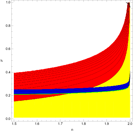
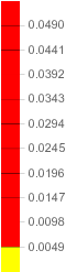
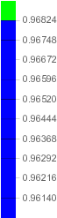
Moreover, by fixing $\tilde{\lambda}\sim 10^{9}$, $V_{0}\sim 0.5$, $N=60$, and allowing $n$ and $\mu$ to vary freely, recalling that $3/2<n<2$, in Fig. 2 we present the contour plots of the spectral index (blue contours) and the contour of the tensor-to-scalar ratio (red and yellow contours). For the spectral index the blue contours correspond to the values in the range $n_{s}=[0.9607,0.9691]$, while for the tensor-to-scalar ratio, the contours correspond to values less than $r\sim 0.054$. As it can be seen, the simultaneous compatibility of the observational indices with the Planck data is achieved for a wide range of the parameters $\mu$ and $n$, without extreme fine-tuning of the model. The same applies if $V_{0}$ varies and the only constraint of the model is that in all cases, the parameter $\tilde{\lambda}$ must take large values of the order $\tilde{\lambda}\sim 10^{9}$.

The present theoretical framework can easily accommodate an $f(R)$ gravity term that can drive the dark energy era. Indeed, this term can be a power-law type term $R^{m}$ which can be chosen to be subleading compared to the term $R^{n}$ appearing in the action (1), for example by choosing the exponent $m$ to be less than unity. This term primordially would be subleading then, thus it would not affect significantly the evolution, however it would affect in a dominant way the late-time evolution. This type of models were considered for example in Capozziello:2006uv; Odintsov:2019evb; Oikonomou:2020qah, and it is always timely to consider power-law higher curvature corrections in order to account for dark energy effects. In the same spirit, one could in principle investigate whether the Swampland criteria are affected by the combined presence of the power-law $f(R)$ gravity Benetti:2019smr and the scalar field. In our case, the task would be more involved compared to the pure $f(R)$ gravity case Benetti:2019smr, since in our case the Einstein frame version of the theory would contain two scalar fields, but this Swampland study would be interesting to investigate in a future work.

At this point let us discuss in some detail the main motivation for choosing an $R^{n}$ gravity in the presence of a single scalar field, instead of choosing for example the $R^{2}$ model to be the dominant curvature term during inflation. Actually, in Ref. Gundhi:2020zvb the scalaron Higgs model was studied. The starting point was a similar to ours Jordan frame action, containing the $R^{2}$ model plus the Higgs scalar field gravitational action. The approach adopted in Ref. Gundhi:2020zvb was quite inceptive since the Jordan frame theory was transformed to the Einstein frame thus a two scalar field Einstein frame theory was obtained. Accordingly the study was performed in the presence of two scalar field. In our approach we remained in the Jordan frame for three main reasons which we quote:

• •

  Firstly the Jordan frame power law $f(R)$ gravity of the form $\sim R^{n}$ with $1<n<2$, in the absence of the scalar field is not a viable theory, since it fails to generate a tensor-to-scalar ratio which is compatible with the latest Planck data. Thus, in contrast to the $R^{2}$ model, the power-law $R^{n}$ model is not a viable theory by itself. Below we shall quote in brief why the vacuum $R^{n}$ theory without the scalar field is not a viable theory.

• •

  Secondly, if we add a scalar field in the Jordan frame, the Jordan frame power-law $R^{n}$ theory is revived and as we showed the combined theory is compatible with the Planck data.

• •

  Thirdly, the study was performed in such a way so that all the equations of motion, the observational indices, the Hubble rate and the slow-roll indices can be expressed in terms of the scalar field. This is because the dominant contribution of the power-law $R^{n}$ gravity basically alters the first Friedmann equation, which in our case is,

  $$H^{2}=\left(\frac{\kappa^{2}V(\varphi)}{\beta}\right)^{\frac{1}{n}}\,,$$

  (41)

  instead of the usual Friedman equation for the canonical scalar field theory,

  $$H^{2}=\frac{\kappa^{2}V(\varphi)}{3}\,.$$

  (42)

  Thus technically, the contribution of the power-law $f(R)$ is the altering of the cosmological equations of motion, and the original Jordan frame $R^{n}$ scalar field theory can be treated as a single scalar field theory with different equations of motion compared to the single scalar field theory. With this technique, the complicated initial Jordan frame $f(R,\phi)$ theory is technically transformed to a single scalar field theory with different equations of motion compared to the ones in the absence of the power-law $f(R)$ gravity term. This is the difference of our approach with Ref. Gundhi:2020zvb, where a two scalar field theory was obtained. Let us also note that in our framework, one may also choose $n=2$, so the $R^{2}$ model plus scalar field can be obtained. However, the $R^{2}$ model is already successful phenomenologically, in contrast to the power-law model with $1<n<2$, thus the latter is more motivated to be studied, since in our approach it becomes revived.

Let us now demonstrate in brief the non-viability of the power-law $f(R)$ gravity model in the absence of the scalar field. Consider,

$$f(R)=R+\beta R^{n}\,,$$

(43)

for $n\neq 2$. The first Friedman equation of the vacuum $f(R)$ gravity is,

$$3H^{2}F=\frac{RF-f}{2}-3H\dot{F}\,,$$

(44)

where $F=\frac{\partial f}{\partial R}$. During inflation, by $F\sim n\beta R^{n-1}$ so the Friedman equation (44) becomes,

$\displaystyle 3H^{2}n\beta R^{n-1}=\frac{\beta(n-1)R^{n-1}}{2}-3n(n-1)\beta HR^{n-2}\dot{R}\,,$

(45)

and due to the fact that $R=12H^{2}+6\dot{H}$, which during inflation becomes at leading order $R\sim 12H^{2}$ and $\dot{R}\sim 24H\dot{H}$, the Friedman equation (45) becomes after some algebra,

$$3H^{2}n\beta\simeq 6\beta(n-1)H^{2}-6n\beta(n-1)\dot{H}+3\beta(n-1)\dot{H}\,,$$

(46)

which when solved yields,

$$H(t)=\frac{-2n^{2}+3n-1}{(n-2)t}\,.$$

(47)

The above Hubble rate describes an accelerating expansion only for $1.36<n<2$. Using the Hubble rate of Eq. (47), the slow-roll indices $\epsilon_{i}$, $i=1,..,4$ can be calculated for the $f(R)$ gravity model (43), and these are,

$$\epsilon_{1}=\frac{n-2}{1-3n+2n^{2}},\,\,\,\epsilon_{2}\simeq 0,\,\,\,\epsilon_{3}=(n-1)\epsilon_{1},\,\,\,\epsilon_{4}=\frac{n-2}{n-1}\,,$$

(48)

Recall the spectral index and the tensor-to-scalar ratio of a vacuum $f(R)$ gravity are reviews1; reviews2,

$$n_{s}=1-6\epsilon_{1}-2\epsilon_{4},\,\,\,r=48\epsilon_{1}^{2}\,.$$

(49)

The only value of the exponent $n$ that can render the spectral index compatible with the Planck data is $n=1.81$, however for this value, the tensor-to-scalar ratio becomes $r=0.13$ which is incompatible with the observational data of Planck Akrami:2018odb. Thus the vacuum power-law Jordan frame $f(R)$ gravity model without the scalar field is incompatible with the Planck data. Let us also note that the scalar power-law model (36) is not compatible with the Planck data for $\mu\leq 2$, thus with our framework we produced a viable phenomenology combining two models which were incompatible with observations otherwise.

In this work we introduced a modified canonical scalar field inflationary theoretical framework, for which the dominant curvature term is not the Ricci scalar, as in Einstein-Hilbert gravity, but a power-law term $\sim R^{n}$, with $3/2<n<2$. This dominance of the power-law term over the Einstein-Hilbert term eventually modifies the field equations and affects significantly the slow-roll evolution of the canonical scalar field. We examined how the field equations become when the dominant curvature term is the power-law one, and by applying the slow-roll conditions for both the Hubble rate and for the scalar field, we were able to express the Friedmann and the Raychaudhuri equations as functions of the scalar field. We calculated the slow-roll indices for the resulting theory and we demonstrated that when the slow-roll conditions hold true, these can be expressed in terms of the slow-roll index $\epsilon_{1}$. Accordingly, we gave exact expressions for the spectral index and for the tensor-to-scalar ratio, which have quite elegant final functional forms, again expressed in terms of the slow-roll index $\epsilon_{1}$ and the second derivative of the scalar potential with respect to the scalar field. We used a simple power-law scalar potential in order to examine the phenomenological viability of the model, and we demonstrated that the model can be compatible with the latest Planck data. In conclusion, the unified framework of the power-law $f(R)$ gravity and of the canonical scalar field, makes possible to obtain phenomenologically viable models which were not viable in the absence of either the scalar field or the power-law $f(R)$ gravity term. For example the simple power-law $f(R)$ gravity model is not compatible with the observational data, and also the power-law scalar model in the absence of the $f(R)$ gravity term, is not in general compatible with the Planck data, and it is compatible for very specific values of the scalar field exponent. Thus the unified theoretical framework we introduced, offers many possibilities for realizing viable inflationary phenomenologies. A mentionable feature of our model is that it falls in the same category as the models studied in Ref. delCampo:2012qb, where the Friedmann equation has the general form $F(H)=\frac{\kappa^{2}V(\phi)}{3}$ in the slow-roll approximation. Such generalized form of the Friedmann equation can be obtained not only by using extra-dimensional frameworks, but also from leading order curvature terms during the inflationary era, as we showed with this work.

References

- (1) A. D. Linde, Lect. Notes Phys. 738 (2008) 1 [arXiv:0705.0164 [hep-th]].
- (2) D. S. Gorbunov and V. A. Rubakov, “Introduction to the theory of the early universe: Cosmological perturbations and inflationary theory,” Hackensack, USA: World Scientific (2011) 489 p;
- (3) A. Linde, arXiv:1402.0526 [hep-th];
- (4) D. H. Lyth and A. Riotto, Phys. Rept. 314 (1999) 1 [hep-ph/9807278].
- (5) Y. Akrami et al. [Planck Collaboration], arXiv:1807.06211 [astro-ph.CO].
- (6) M. Kamionkowski and E. D. Kovetz, Ann. Rev. Astron. Astrophys. 54 (2016) 227 doi:10.1146/annurev-astro-081915-023433 [arXiv:1510.06042 [astro-ph.CO]].
- (7) R. H. Brandenberger, arXiv:1206.4196 [astro-ph.CO].
- (8) R. Brandenberger and P. Peter, arXiv:1603.05834 [hep-th].
- (9) D. Battefeld and P. Peter, Phys. Rept. 571 (2015) 1 [arXiv:1406.2790 [astro-ph.CO]].
- (10) M. Novello and S. E. P. Bergliaffa, Phys. Rept. 463 (2008) 127 [arXiv:0802.1634 [astro-ph]].
- (11) Y. F. Cai, Sci. China Phys. Mech. Astron. 57 (2014) 1414 doi:10.1007/s11433-014-5512-3 [arXiv:1405.1369 [hep-th]].
- (12) J. de Haro and Y. F. Cai, Gen. Rel. Grav. 47 (2015) no.8, 95 [arXiv:1502.03230 [gr-qc]].
- (13) J. L. Lehners, Class. Quant. Grav. 28 (2011) 204004 [arXiv:1106.0172 [hep-th]].
- (14) J. L. Lehners, Phys. Rept. 465 (2008) 223 [arXiv:0806.1245 [astro-ph]].
- (15) Y. K. E. Cheung, C. Li and J. D. Vergados, arXiv:1611.04027 [astro-ph.CO].
- (16) Y. F. Cai, A. Marciano, D. G. Wang and E. Wilson-Ewing, Universe 3 (2016) no.1, 1 doi:10.3390/universe3010001 [arXiv:1610.00938 [astro-ph.CO]].
- (17) S. D. Odintsov, V. K. Oikonomou, F. P. Fronimos and K. V. Fasoulakos, Phys. Rev. D 102 (2020) no.10, 104042 doi:10.1103/PhysRevD.102.104042 [arXiv:2010.13580 [gr-qc]].
- (18) G. Aad et al. [ATLAS], Phys. Lett. B 716 (2012), 1-29 doi:10.1016/j.physletb.2012.08.020 [arXiv:1207.7214 [hep-ex]].
- (19) J. c. Hwang and H. Noh, Phys. Rev. D 71 (2005) 063536 doi:10.1103/PhysRevD.71.063536 [gr-qc/0412126].
- (20) S. Nojiri, S. D. Odintsov and M. Sami, Phys. Rev. D 74 (2006) 046004 doi:10.1103/PhysRevD.74.046004 [hep-th/0605039].
- (21) G. Cognola, E. Elizalde, S. Nojiri, S. Odintsov and S. Zerbini, Phys. Rev. D 75 (2007) 086002 doi:10.1103/PhysRevD.75.086002 [hep-th/0611198].
- (22) S. Nojiri, S. D. Odintsov and M. Sasaki, Phys. Rev. D 71 (2005) 123509 doi:10.1103/PhysRevD.71.123509 [hep-th/0504052].
- (23) S. Nojiri and S. D. Odintsov, Phys. Lett. B 631 (2005) 1 doi:10.1016/j.physletb.2005.10.010 [hep-th/0508049].
- (24) M. Satoh, S. Kanno and J. Soda, Phys. Rev. D 77 (2008) 023526 doi:10.1103/PhysRevD.77.023526 [arXiv:0706.3585 [astro-ph]].
- (25) K. Bamba, A. N. Makarenko, A. N. Myagky and S. D. Odintsov, JCAP 1504 (2015) 001 doi:10.1088/1475-7516/2015/04/001 [arXiv:1411.3852 [hep-th]].
- (26) Z. Yi, Y. Gong and M. Sabir, Phys. Rev. D 98 (2018) no.8, 083521 doi:10.1103/PhysRevD.98.083521 [arXiv:1804.09116 [gr-qc]].
- (27) Z. K. Guo and D. J. Schwarz, Phys. Rev. D 80 (2009) 063523 doi:10.1103/PhysRevD.80.063523 [arXiv:0907.0427 [hep-th]].
- (28) Z. K. Guo and D. J. Schwarz, Phys. Rev. D 81 (2010) 123520 doi:10.1103/PhysRevD.81.123520 [arXiv:1001.1897 [hep-th]].
- (29) P. X. Jiang, J. W. Hu and Z. K. Guo, Phys. Rev. D 88 (2013) 123508 doi:10.1103/PhysRevD.88.123508 [arXiv:1310.5579 [hep-th]].
- (30) P. Kanti, R. Gannouji and N. Dadhich, Phys. Rev. D 92 (2015) no.4, 041302 doi:10.1103/PhysRevD.92.041302 [arXiv:1503.01579 [hep-th]].
- (31) C. van de Bruck, K. Dimopoulos, C. Longden and C. Owen, arXiv:1707.06839 [astro-ph.CO].
- (32) P. Kanti, J. Rizos and K. Tamvakis, Phys. Rev. D 59 (1999) 083512 doi:10.1103/PhysRevD.59.083512 [gr-qc/9806085].
- (33) E. O. Pozdeeva, M. R. Gangopadhyay, M. Sami, A. V. Toporensky and S. Y. Vernov, arXiv:2006.08027 [gr-qc].
- (34) I. Fomin, arXiv:2004.08065 [gr-qc].
- (35) M. De Laurentis, M. Paolella and S. Capozziello, Phys. Rev. D 91 (2015) no.8, 083531 doi:10.1103/PhysRevD.91.083531 [arXiv:1503.04659 [gr-qc]].
- (36) S. Chervon, I. Fomin, V. Yurov and A. Yurov, doi:10.1142/11405
- (37) K. Nozari and N. Rashidi, Phys. Rev. D 95 (2017) no.12, 123518 doi:10.1103/PhysRevD.95.123518 [arXiv:1705.02617 [astro-ph.CO]].
- (38) S. D. Odintsov and V. K. Oikonomou, Phys. Rev. D 98 (2018) no.4, 044039 doi:10.1103/PhysRevD.98.044039 [arXiv:1808.05045 [gr-qc]].
- (39) S. Kawai, M. a. Sakagami and J. Soda, Phys. Lett. B 437, 284 (1998) doi:10.1016/S0370-2693(98)00925-3 [gr-qc/9802033].
- (40) Z. Yi and Y. Gong, Universe 5 (2019) no.9, 200 doi:10.3390/universe5090200 [arXiv:1811.01625 [gr-qc]].
- (41) C. van de Bruck, K. Dimopoulos and C. Longden, Phys. Rev. D 94 (2016) no.2, 023506 doi:10.1103/PhysRevD.94.023506 [arXiv:1605.06350 [astro-ph.CO]].
- (42) B. Kleihaus, J. Kunz and P. Kanti, arXiv:1910.02121 [gr-qc].
- (43) A. Bakopoulos, P. Kanti and N. Pappas, Phys. Rev. D 101 (2020) no.4, 044026 doi:10.1103/PhysRevD.101.044026 [arXiv:1910.14637 [hep-th]].
- (44) K. i. Maeda, N. Ohta and R. Wakebe, Eur. Phys. J. C 72 (2012) 1949 doi:10.1140/epjc/s10052-012-1949-6 [arXiv:1111.3251 [hep-th]].
- (45) A. Bakopoulos, P. Kanti and N. Pappas, arXiv:2003.02473 [hep-th].
- (46) W. Ai, [arXiv:2004.02858 [gr-qc]].
- (47) S. D. Odintsov and V. K. Oikonomou, Phys. Lett. B 797 (2019) 134874 doi:10.1016/j.physletb.2019.134874 [arXiv:1908.07555 [gr-qc]].
- (48) V. K. Oikonomou and F. P. Fronimos, [arXiv:2007.11915 [gr-qc]].
- (49) S. D. Odintsov, V. K. Oikonomou and F. P. Fronimos, Annals Phys. 420 (2020), 168250 doi:10.1016/j.aop.2020.168250 [arXiv:2007.02309 [gr-qc]].
- (50) V. K. Oikonomou and F. P. Fronimos, [arXiv:2006.05512 [gr-qc]].
- (51) S. D. Odintsov and V. K. Oikonomou, Phys. Lett. B 805 (2020), 135437 doi:10.1016/j.physletb.2020.135437 [arXiv:2004.00479 [gr-qc]].
- (52) S. D. Odintsov, V. K. Oikonomou and F. P. Fronimos, [arXiv:2003.13724 [gr-qc]].
- (53) S. D. Odintsov, V. K. Oikonomou, F. P. Fronimos and S. A. Venikoudis, Phys. Dark Univ. 30 (2020), 100718 doi:10.1016/j.dark.2020.100718 [arXiv:2009.06113 [gr-qc]].
- (54) R. Easther and K. i. Maeda, Phys. Rev. D 54 (1996) 7252 doi:10.1103/PhysRevD.54.7252 [hep-th/9605173].
- (55) I. Antoniadis, J. Rizos and K. Tamvakis, Nucl. Phys. B 415 (1994) 497 doi:10.1016/0550-3213(94)90120-1 [hep-th/9305025].
- (56) I. Antoniadis, C. Bachas, J. R. Ellis and D. V. Nanopoulos, Phys. Lett. B 257 (1991), 278-284 doi:10.1016/0370-2693(91)91893-Z
- (57) P. Kanti, N. Mavromatos, J. Rizos, K. Tamvakis and E. Winstanley, Phys. Rev. D 54 (1996), 5049-5058 doi:10.1103/PhysRevD.54.5049 [arXiv:hep-th/9511071 [hep-th]].
- (58) P. Kanti, N. Mavromatos, J. Rizos, K. Tamvakis and E. Winstanley, Phys. Rev. D 57 (1998), 6255-6264 doi:10.1103/PhysRevD.57.6255 [arXiv:hep-th/9703192 [hep-th]].
- (59) S. Nojiri, S. D. Odintsov and V. K. Oikonomou, Phys. Rept. 692 (2017) 1 [arXiv:1705.11098 [gr-qc]].
- (60)
S. Capozziello, M. De Laurentis,
Phys. Rept. 509, 167 (2011);
V. Faraoni and S. Capozziello, The landscape beyond Einstein gravity, in Beyond Einstein Gravity 828 (Springer, Dordrecht, 2010), Vol. 170, pp.59-106. - (61) S. Nojiri, S.D. Odintsov, Phys. Rept. 505, 59 (2011);
- (62) A. de la Cruz-Dombriz and D. Saez-Gomez, Entropy 14 (2012) 1717 [arXiv:1207.2663 [gr-qc]].
- (63) Introduction to Cosmic Inflation and Dark Energy, Konstantinos Dimopoulos, CRC Press 2020
- (64) N. Aghanim et al. [Planck], Astron. Astrophys. 641 (2020), A6 doi:10.1051/0004-6361/201833910 [arXiv:1807.06209 [astro-ph.CO]].
- (65) R. R. Caldwell, M. Kamionkowski and N. N. Weinberg, Phys. Rev. Lett. 91 (2003), 071301 doi:10.1103/PhysRevLett.91.071301 [arXiv:astro-ph/0302506 [astro-ph]].
- (66) V. Oikonomou, “Rectifying an Inconsistency in Gravity Inflation,” European Physics Letters in press, [arXiv:2004.10778 [gr-qc]].
- (67) A. Gundhi and C. F. Steinwachs, [arXiv:2011.09485 [hep-th]].
- (68) S. Capozziello, V. F. Cardone and A. Troisi, JCAP 08 (2006), 001 doi:10.1088/1475-7516/2006/08/001 [arXiv:astro-ph/0602349 [astro-ph]].
- (69) S. D. Odintsov and V. K. Oikonomou, Phys. Rev. D 99 (2019) no.10, 104070 doi:10.1103/PhysRevD.99.104070 [arXiv:1905.03496 [gr-qc]].
- (70) V. K. Oikonomou, Phys. Rev. D 103 (2021) no.4, 044036 doi:10.1103/PhysRevD.103.044036 [arXiv:2012.00586 [astro-ph.CO]].
- (71) M. Benetti, S. Capozziello and L. L. Graef, Phys. Rev. D 100 (2019) no.8, 084013 doi:10.1103/PhysRevD.100.084013 [arXiv:1905.05654 [gr-qc]].
- (72) S. del Campo, JCAP 12 (2012), 005 doi:10.1088/1475-7516/2012/12/005 [arXiv:1212.1315 [astro-ph.CO]].