Generalizing Dynamic Mode Decomposition: Balancing Accuracy and Expressiveness in Koopman Approximations
Abstract
This paper tackles the data-driven approximation of unknown dynamical systems using Koopman-operator methods. Given a dictionary of functions, these methods approximate the projection of the action of the operator on the finite-dimensional subspace spanned by the dictionary. We propose the Tunable Symmetric Subspace Decomposition algorithm to refine the dictionary, balancing its expressiveness and accuracy. Expressiveness corresponds to the ability of the dictionary to describe the evolution of as many observables as possible and accuracy corresponds to the ability to correctly predict their evolution. Based on the observation that Koopman-invariant subspaces give rise to exact predictions, we reason that prediction accuracy is a function of the degree of invariance of the subspace generated by the dictionary and provide a data-driven measure to measure invariance proximity. The proposed algorithm iteratively prunes the initial function space to identify a refined dictionary of functions that satisfies the desired level of accuracy while retaining as much of the original expressiveness as possible. We provide a full characterization of the algorithm properties and show that it generalizes both Extended Dynamic Mode Decomposition and Symmetric Subspace Decomposition. Simulations on multiple systems show the effectiveness of the proposed methods in producing Koopman approximations of tunable accuracy that capture relevant information about the dynamical system.
keywords
Nonlinear system identification, Koopman operator, Dynamic Mode Decomposition, accurate predictionA preliminary version of this paper appeared at the American Control Conference as (Haseli and Cortés 2021a).††address: Department of Mechanical and Aerospace Engineering, University of California, San Diego, {mhaseli,cortes}@ucsd.edu
1 Introduction
Progress in data acquisition and labeling, along with widespread access to high-performance computing capabilities for storing, processing, and data analysis, has resulted in a surge of activity in learning and modeling of dynamical phenomena across multiple domains. In this context, the importance of identification techniques that yield tractable representations of nonlinear dynamics rooted at a solid theoretical framework cannot be overemphasized. One such technique is Koopman operator theory which, instead of prescribing the evolution of system trajectories as state-space models do, describes the evolution of functions defined over the state space (a.k.a. observables). The infinite-dimensional nature of the operator has prevented its widespread use due to the lack of computational methods to represent it. Extended dynamic mode decomposition (EDMD) addresses this by employing data from the dynamics to approximate the projection of the action of the Koopman operator on a finite-dimensional subspace spanned by a predefined dictionary of functions.
Despite EDMD’s success, it is still not well understood how to choose dictionaries that both capture relevant information about the dynamics and are able to accurately predict its evolution. Prediction accuracy is related to the degree of invariance, with respect to the operator, of the subspace generated by the dictionary and, in fact, can be improved by selectively pruning its functions. Such process, however, impacts expressiveness, understood as the ability of the dictionary to describe the evolution of as many observables as possible. This paper is motivated by the need to address the accuracy-expressiveness trade-off in dictionary selection.
Literature Review: Given a dynamical system, its associated Koopman operator (Koopman 1931; Koopman and Neumann 1932) is a linear operator characterizing the effect of the dynamics on functions in a (generally infinite-dimensional) linear function space. The values of its eigenfunctions also evolve linearly in time on the trajectories of the system. These properties enable the use of the spectral properties of the operator to process data from dynamical systems using efficient linear algebraic methods fully compatible with the arithmetic operations of digital computers (Mezić 2005; Budišić et al. 2012). This has led to many applications in fluid dynamics (Rowley et al. 2009), model reduction (Mezić 2005), and control, including controller synthesis (Choi et al. 2020; Folkestad et al. 2020; Goswami and Paley 2022), model predictive control (Korda and Mezić 2018a; Son et al. 2020), control of PDEs (Peitz and Klus 2019), and robotic applications (Mamakoukas et al. 2019; Zinage and Bakolas 2022).
The infinite-dimensional nature of the Koopman operator is an impediment to its direct implementation on digital computers. A popular way to find finite-dimensional representations of the operator is through Dynamic Mode Decomposition (DMD) and its variants, initially developed to extract dynamical information from data about fluid flows (Schmid 2010; Tu et al. 2014). Williams et al. 2015 developed the Extended Dynamic Mode Decomposition (EDMD) algorithm, a variant of DMD capable of approximating the projection of the action of the Koopman operator from data on a finite-dimensional space spanned by a chosen dictionary of functions. Korda and Mezić 2018b formally established the convergence of the EDMD approximation to the projection of the action of the operator on the span of the dictionary. Recently, Lu and Tartakovsky 2020 analyzed the accuracy of long-term prediction by DMD and its variants. Mamakoukas et al. 2021 used a Taylor expansion method to enrich the dictionary for EDMD to achieve lower errors in long-term predictions. Zhang and Zuazua 2021 used finite element methods to learn Koopman approximations with accuracy bounds quantifying their quality. This work also provided a variant of EDMD to learn the Koopman generator combined with finite element methods. Nüske et al. 2021 provided several probabilistic bounds for approximation of the Koopman operator based on the availability of only finitely many data points both for deterministic and stochastic systems. It is worth mentioning that (E)DMD captures valuable information about stochastic dynamical systems (Williams et al. 2015; Klus et al. 2020); however, it is sensitive to the existence of measurement noise in the available data. Dawson et al. 2016 and Haseli and Cortés 2019 provide methods to deal with measurement noise in data for DMD and EDMD, respectively.
In general, given an arbitrary dictionary, there is no guarantee that EDMD provides an accurate approximation for all the observables in the span of the dictionary. This has resulted in the search for dictionaries that span invariant subspaces (Brunton et al. 2016a) under the Koopman operator, on which the EDMD approximation is exact. The work (Johnson and Yeung 2018) introduces a class of logistic functions to approximate Koopman-invariant subspaces for systems whose dynamics are known. On the other hand, given unknown systems and using data sampled from their trajectories, Koopman-invariant subspaces are approximated using neural networks in (Takeishi et al. 2017; Lusch et al. 2018; Yeung et al. 2019; Otto and Rowley 2019) and sparsity-promoting methods in (Pan et al. 2021). The works by (Kaiser et al. 2021; Korda and Mezic 2020) directly approximate Koopman eigenfunctions, which naturally span Koopman-invariant subspaces. These data-driven methods do not provide theoretical guarantees for the resulting approximations. Given the importance of such guarantees, our previous work (Haseli and Cortés 2022; Haseli and Cortés 2021b) has provided necessary and almost surely sufficient conditions for the identification of the maximal Koopman-invariant subspace and all Koopman eigenfunctions in an arbitrary finite-dimensional function space. We have also provided approximations to identify subspaces that are close to being invariant for cases when the maximal Koopman-invariant subspace does not capture enough information about the dynamics.
It is important to note that the existence of finite-dimensional Koopman-invariant subspaces containing the states of the system is not guaranteed (Brunton et al. 2016a). However, invariant subspaces still contain Koopman eigenfunctions, and can capture relevant information about the vector field, physical constraints, conservation laws, stability, and even the construction of Lyapunov functions, see e.g., (Mauroy and Mezić 2016). Nonetheless, in some applications, one can tolerate a certain level of inaccuracy in order to capture a more diverse function space that is not necessarily Koopman invariant but captures important variables such as the states of the system.
Statement of Contributions: We consider the problem of data-driven identification of finite-dimensional spaces that are close, with tunable accuracy, to being invariant under the action of the Koopman operator. Our main result, illustrated in Figure 1, consists of the synthesis of a computational procedure, termed Tunable Symmetric Subspace Decomposition (T-SSD), that given an arbitrary finite-dimensional function space, balances the trade-off between the expressiveness11 1 We note that notions of expresiveness different that the one adopted here are also possible. For instance, and although out of the scope of the paper, expresiveness could also be understood as the ability of the dictionary to describe specific finitely many predefined observables of interest, such as state variables, in a given set of coordinates. of its subspaces and the accuracy of the Koopman approximations on them.
The roadmap of supporting contributions leading to the design and full characterization of T-SSD is as follows. Our first contribution builds on the observation that the proximity of a function space to being invariant is a measure of its (and consequently its members’) prediction accuracy under finite-dimensional Koopman approximations, as an exact invariant subspace leads to exact predictions of the evolution of observables. We introduce the novel notion of -apart spaces to measure invariance proximity using data snapshots sampled from the trajectories of the unknown dynamics. Using this notion, and given an arbitrary finite-dimensional function space spanned by a dictionary of functions, we formulate our objective as that of finding a parametric family of subspaces whose value of the parameter determines the desired level of invariance proximity. This parametric family can be viewed as balancing invariance proximity (i.e., prediction accuracy) and the dimension of the subspace (i.e., expressiveness).
Given a desired accuracy parameter, our second contribution is the design of T-SSD as an algorithmic procedure that finds a function space satisfying the desired accuracy by iteratively removing the functions in the span of the original dictionary that violate the desired accuracy. We show that T-SSD terminates in a finite number of iterations and characterize its computational complexity. Moreover, we show that its identified subspaces contain the maximal Koopman-invariant subspace and all Koopman eigenfunctions in the span of the original dictionary. We also show that the accuracy parameter bounds the relative root mean square prediction error for all (uncountably many) functions in the identified subspace. This advantage of the T-SSD algorithm in deriving accuracy bounds on the prediction of individual functions independently of linear changes of coordinates stems from focusing on the subspaces instead of their basis. Our next contribution establishes that both Extended Dynamic Mode Decomposition and Symmetric Subspace Decomposition algorithms are particular cases of T-SSD, cf. Figure 1.
Our final contribution is a computationally efficient version of T-SSD with drastically lower computational complexity when the number of data snapshots is significantly larger than the dimension of the original dictionary. We illustrate in simulation the effectiveness of T-SSD in identifying informative Koopman approximations of tunable accuracy.
2 Preliminaries
Here, we introduce the notation used in the paper and provide a brief overview of Koopman operator theory, extended dynamic mode decomposition (EDMD), and symmetric subspace decomposition (SSD).
2.1 Notation
We let , , , and represent the sets of real, complex, nonnegative integer, and natural numbers respectively. Given a matrix , we denote its transpose, conjugate transpose, pseudo-inverse, range space, and Frobenius norm by , , , , and respectively. In addition, , , , and represent its set of columns, set of rows, number of columns, and number of rows. Also if is a nonsingular square matrix, denotes its inverse. Given and , we use to represent the matrix formed by their side by side concatenation. We denote by and , the zero matrix and the identity matrix of size respectively (we omit the indices when the context is clear). Given a vector , denotes its 2-norm.
We denote by the vector space over spanned by . Given functions , is the function space formed by all functions in the form of with . For a vector space , denotes the orthogonal projection operator on . For convenience, we denote the orthogonal projection operator on the range space of a matrix by , which takes the form , for . For vectors , indicates that and are orthogonal. Given vector spaces , denotes that the vector spaces are orthogonal, i.e., all vectors in are orthogonal to all vectors in . We define the sum of vector spaces by . Given sets , we denote their union and intersection by and respectively. Given functions , , denotes their composition.
2.2 Koopman Operator
Our exposition follows Budišić et al. 2012: given the discrete-time dynamics
| (1) |
defined on the state space and a linear space of functions defined over the field and closed under composition with , the Koopman operator associated with (1) is defined as . The functions in are called observables. As a consequence of the linearity of , the Koopman operator is spatially linear, i.e.,
| (2) |
for any and . The linearity of the Koopman operator paves the way for defining its eigendecomposition. Formally, a function is an eigenfunction of the Koopman operator with eigenvalue if
| (3) |
The eigenfunctions of the Koopman operator evolve linearly in time on the trajectories of (1),
| (4) |
The linear temporal evolution of eigenfunctions combined with (2) make the Koopman operator a powerful tool for linear prediction of the functions’ values on the trajectories of the (generally nonlinear) dynamical system (1). Formally, given a function , where and are eigenfunctions of with eigenvalues , one can predict the values of on the trajectory starting from initial condition as
| (5) |
Finally, a subspace is Koopman-invariant if for every , we have . Trivially, any subspace spanned by Koopman eigenfunctions is Koopman invariant.
2.3 Extended Dynamic Mode Decomposition
In general, the Koopman operator is infinite dimensional. Moreover, in many practical data-driven applications, the dynamical system is unknown and only data from some trajectories is available. These issues motivate the use of data-driven methods to approximate the effect of the Koopman operator on finite-dimensional subspaces, as we discuss next. Here, we recall the Extended Dynamic Mode Decomposition (EDMD) method following Williams et al. 2015. EDMD uses data from the trajectories of the system to approximate the action of the Koopman operator on a predefined function space. The first ingredient of EDMD is the data matrices containing data snapshots, where corresponding rows of characterize two consecutive points on a trajectory of the system. Formally,
| (6) |
where and are the th rows of and respectively. The second ingredient of EDMD is a dictionary of functions, denoted as
| (7) |
where for all . The dictionary spans a finite-dimensional space of functions over , and its elements can be complex-valued functions in general. However, since the system is defined over the state space , complex Koopman eigenfunctions form complex conjugate pairs which can be fully represented by a pair of real-valued functions. For this reason, and without loss of generality, we use real-valued functions as dictionary elements.
EDMD formulates a least-squares optimization to find the best fit for the linear evolution of the dictionary functions on the data. If we denote the effect of the dictionary on an arbitrary data matrix by , where corresponds to the th row of , then one can write the EDMD’s optimization problem in compact form as
| (8) |
whose closed-form solution is
| (9) |
approximates the projection of the action of the Koopman operator on as follows. Under the identification of with defined by , this approximation takes the form
| (10) |
As a result, for the function , one can define the EDMD’s approximation of as
| (11) |
It is important to note that can be viewed as the -orthogonal projection of on given an empirical measure defined based on the rows of (Klus et al. 2016; Korda and Mezić 2018b). Moreover, the eigendecomposition of provides insight into the eigendecomposition of the Koopman operator. Formally, given an eigenpair of , one approximates an eigenfunction of the Koopman operator with eigenvalue as
| (12) |
Note that the EDMD predictor in (11) applied to the eigenfunction in (12) leads to , which is in agreement with the linear evolution (4) of Koopman eigenfunctions. Note that EDMD provides Koopman (generalized) eigenfunction approximations even if the Koopman operator does not have eigenfunctions in the span of the dictionary. If the dictionary spans a Koopman-invariant subspace, then EDMD completely captures the behavior of the Koopman operator (and all its eigenfunctions) on . As a result, , and (11) provides exact prediction, independently of the data used for EDMD’s training.
We refer the reader to (Korda and Mezić 2018b) for asymptotic convergence results as , concerning capturing the spectrum of the Koopman operator as well as the finite-horizon prediction of EDMD for observables in . It is essential to keep in mind that the aforementioned asymptotic convergence results do not imply that a larger dictionary is necessarily closer to being invariant under the Koopman operator. In general, asymptotic behavior requires a sufficiently large dictionary; however, unless other properties (e.g., monotonicity) exist, the dictionary’s quality (in terms of prediction accuracy) might deteriorate by adding more functions. We illustrate this point in the following example.
Example 2.1
(A Larger Dictionary is Not Necessarily Better): Consider the linear system with state space . Consider the dictionaries, and . Clearly, . However, is invariant under the Koopman operator and EDMD’s prediction (which coincides with the dynamics) is exact. On the other hand, despite being a larger dictionary (and containing ), EDMD with dictionary does not lead to accurate predictions on . The reason for this issue is that by adding the function to dictionary , we break the invariance of its span, leading to a larger space which is not invariant.
A final note regarding EDMD is that it is not designed to work with data corrupted with measurement noise. Hence, data pre-processing might be needed to take full advantage of the methods proposed in the paper, which rely on EDMD.
2.4 Symmetric Subspace Decomposition
In general, since the true system dynamics is unknown, choosing a dictionary that spans a Koopman-invariant subspace is challenging. This justifies the importance of developing data-driven methods that aid in this task. Here, we recall the Symmetric Subspace Decomposition (SSD) algorithm following Haseli and Cortés 2022. Starting from a dictionary and data snapshots , the SSD algorithm, cf. Algorithm 1, finds a basis for the maximal Koopman-invariant subspace in . To achieve this goal, SSD relies on the following.
Assumption 2.2
(Full Rank Dictionary Matrices): The matrices and have full column rank.
Assumption 2.2 rules out the case of redundant dictionary elements by making sure its functions are linearly independent. Moreover, it requires the data snapshots to be sampled in a way that reflects this fact.
The SSD algorithm provides an iterative approach to prune the dictionary at each iteration by removing the functions that do not correspond to linear evolutions. The SSD algorithm terminates after finite iterations and its output satisfies the following properties.
Theorem 2.3
(SSD Output (Haseli and Cortés 2022, Theorem 5.1)): Suppose that Assumption 2.2 holds. Then,
- a.
is either or has full column rank;
- b.
satisfies ;
- c.
the subspace is maximal, in the sense that, for any matrix with , we have and .
The dictionary identified by SSD is
| (13) |
Based on Theorem 2.3, spans the largest subspace of on which . One can apply the EDMD algorithm (equations (8)-(9)) on and to find the predictor matrix
| (14) |
The residual error is equal to zero and fully captures the behavior of the available data. Moreover, one can replace and in (11)-(12) by and to define approximated Koopman eigenfunctions and linear predictors for the dynamics. Under reasonable assumptions on the data sampling, is the maximal Koopman-invariant subspace in almost surely and consequently the aforementioned eigenfunctions and predictors are exact for all points (not just on the sampled data) in the state space almost surely. We refer the reader to (Haseli and Cortés 2022) for additional information about the SSD algorithm, its convergence, and its properties regarding the identification of the eigenfunctions of the Koopman operator. We conclude this section by remarking that the SSD algorithm is, in fact, an algebraic search.
Remark 2.4
(SSD is an Efficient Algebraic Subspace Search): One can view the SSD algorithm as an algebraic method that searches through all subspaces of a finite-dimensional vector space of functions. In fact, in Algorithm 1, one can view as the space we search through, and the space (solution of SSD) as the maximal Koopman-invariant subspace (almost surely) in our search space . For example, if use the SSD algorithm on the system in Example 2.1 and set as our search space, we find the subspace , which is Koopman invariant and leads to exact prediction.
3 Problem Statement
We start by noting that one can view the SSD and EDMD methods described in Section 2 as the two extreme cases in the trade-off between prediction accuracy and dictionary expressiveness. This is because, on the one hand, the SSD predictor provides almost surely exact predictions for functions in but, due to the pruning of the original dictionary , this might not be sufficiently expressive to capture the system dynamics. EDMD, on the other hand, provides predictions for all functions in , but there is no guarantee on the accuracy of this prediction.
Our goal is then to explore the accuracy-expressiveness spectrum in-between the extreme cases of SSD and EDMD. To do this, we seek to provide a formal data-driven characterization of how close a function space is to being invariant under the Koopman operator (something we refer to as invariance proximity). Equipped with this notion, we also aim to develop fast algebraic methods that can find finite-dimensional function spaces that meet a desired level of invariance proximity. Throughout the paper we do not assume any information about the dynamical system except the existence of a finite data set of snapshots gathered from its trajectories.
Formally, given the original dictionary defined in (7), data snapshots matrices gathered from the dynamical system (1) defined in (6), and assuming that Assumption 2.2 holds, we seek to:
- a.
provide a measure to quantify the invariance proximity of span of any dictionary with elements in solely based on available data ;
- b.
provide an algebraic algorithm that searches through the subspaces of and finds a dictionary , where meets a desired level of invariance proximity;
- c.
such that contains the maximal Koopman-invariant subspace in .
Requirement (c) ensures the correctness of the algorithmic solution by ensuring the maximal Koopman-invariant subspace and all Koopman eigenfunctions in are captured.
4 -Apart Spaces Measure Invariance Proximity
In this section we provide a quantifiable measure for invariance proximity of a subspace by studying the behavior of EDMD with respect to its dictionary. Since the true system dynamics is unknown, this measure must be based on the available data matrices and . To gain a deeper understanding about the behavior of the data-dictionary pair, we offer the following interpretation of the action of the solution of the optimization (8) as a projection from onto . To see this, let be a vector of the form of . Using (9),
where we have used that is the projection operator on . Using this projection viewpoint alongside (8) reveals that the residual error of EDMD, and consequently its accuracy on the available data, depends of how close the subspaces and are. In fact, note that
- •
- •
instead, if , one can deduce that under Assumption 2.2, and EDMD captures no information about the dynamics. In particular, the residual error amounts to prediction error for .
We illustrate next the aforementioned cases.
Example 4.1
(Dependence of EDMD’s Prediction on Data and Dictionary): Consider the discrete-time system with state space . Suppose that we gather data snapshots () from a single trajectory with length starting from the initial condition . Hence, and . If we choose our dictionary as (which spans a Koopman-invariant subspace), EDMD captures complete information about the dynamics. However, if we remove the constant function from the dictionary, the new dictionary snapshots matrices are equal to and , and span orthogonal subspaces. In this case, and EDMD does not capture any information about the dynamics.
These observations suggests that the proximity of the vector spaces and can be used as a quantifiable characterization for invariance proximity of and consequently the prediction accuracy of EDMD. This motivates the following definition.
Definition 4.2
(-Apart Subspaces): Given , two vector spaces are -apart if , for all .
According to this definition22 2 Note that, unlike Grassmannians, e.g. (Absil et al. 2009), there is no restriction on the dimension of the subspaces in Definition 4.2., the norm of the error induced by projecting a vector belonging to one of the subspaces onto the other subspace is smaller than . Next, we show that this notion fully characterizes equality of spaces with the case .
Lemma 4.3
(0-apart Subspaces are Equal): Vector spaces are 0-apart if and only if .
PROOF.
: Let . By definition, , and hence . Consequently, , showing . The inclusion can be proved analogously, and we conclude .
: Since , for all , we have . Hence, , for all , and the result follows. ∎
The next result shows that all subspaces are -apart.
Lemma 4.4
(Any Two Subspaces are 1-apart): Any two vector spaces are 1-apart.
PROOF.
For any , one can write
where in the last equality we have used the fact that is the projection operator on the orthogonal complement of . One can write a similar argument for , which completes the proof. ∎
Lemmas 4.3-4.4 together imply that the range for the parameter fully characterizes the proximity of any two subspaces. This enables us to use the concept of -apart subspaces on and as a way to quantify the invariance proximity of under the Koopman operator associated with the system (1). Equipped with this, we reformulate next the problems (b)-(c) in Section 3.
Problem 4.5
(Balancing Prediction Accuracy and expressiveness): Given the parameter , find a dictionary with elements in such that
- (b)
and are -apart;
- (c)
contains the maximal Koopman-invariant subspace in .
It is worth mentioning that
captures the invariance proximity, and consequently the prediction accuracy, of . As a result, if we choose in Problem 4.5, the new dictionary would be smaller than , leading to a decrease of the expressiveness of the resulting dictionary. Hence, the choice of parameter strikes a balance between prediction accuracy and expressiveness of the dictionary.
5 Tunable Symmetric Subspace Decomposition
In this section, we design and analyze an algorithm, termed Tunable Symmetric Subspace Decomposition (T-SSD), to address Problem 4.5.
5.1 The T-SSD Algorithm
Given the dictionary and data snapshots , , the problem of finding a dictionary such that and are -apart can be tackled by pruning . We next describe informally the procedure and then formalize it in Algorithm 2.
[Informal description:] The pruning consists of identifying the functions that violate the desired invariance proximity condition and remove them from the span of the dictionary. To identify such functions, we define the projection difference matrix (Step 7 in Algorithm 2)
which is a symmetric matrix with mutually orthogonal eigenvectors spanning (with corresponding real-valued eigenvalues). Interestingly, if all eigenvalues of belong to , then and are -apart. Otherwise, we focus our attention on the smaller subspace of defined by
corresponding to the span of eigenvectors of with eigenvalues in . For practical reasons, we work with a basis for (Step 9 in Algorithm 2). Next, we find the largest dictionary with elements in such that (Steps 11-13 in Algorithm 2). There are two possible outcomes:
- (i)
;
- (ii)
.
Scenario (i) indicates that the dictionary does not need pruning and are -apart (Steps 21-23 in Algorithm 2). On the other hand, scenario (ii) leads to a dictionary of lower dimension. However, it is not guaranteed that and are -apart since is a different dictionary than . Consequently, we re-run the process, starting with the definition of , for the new dictionary . This leads to an iterative implementation that stops when the dictionary cannot be reduced anymore (yielding the desired -apart subspaces).
The formalization of this procedure yields the Tunable Symmetric Subspace Decomposition (T-SSD)33 3 In Algorithms 2-3, the outputs of and are matrices whose columns form orthonormal bases for the null space of and , respectively. in Algorithm 2. We make the following additional observations regarding the use of notation to provide intuition about the algorithm pseudocode: (i) we index the internal matrix variables based on the iteration number (this facilitates later the in-depth algebraic analysis); (ii) noting that, at each iteration, the dictionary elements are linear combinations of the elements of the original dictionary, we represent the dictionary at iteration simply by a matrix , which corresponds to the dictionary ; (iii) using the representation in (ii), we do not need to form the dictionary and apply it on the data matrices and . Instead, the effect of the dictionary at iteration on the data can be represented as and .
Algorithm 3 describes the function in Step 11 of T-SSD: this strategy corresponds to the computation described above of the largest dictionary such that and belong to the reduced subspace . Similarly to Algorithm 2, instead of actually forming the reduced dictionary, Algorithm 3 uses the matrix-based representation of the dictionary. Next, we explain the steps of the algorithm and the reason behind its naming. Given input matrices , , and , Step 7 in Algorithm 3 identifies such that (see Lemma A.1). Then, again in Step 16 the algorithm (by virtue of Lemma A.1) finds the matrix such that . The output matrix (cf. Step 16) then specifies the largest subspaces , both belonging to . Note the symmetry in this specification: if a linear combination of the columns of is in , then the same linear combination of columns of belongs to . Moreover, Algorithm 3 breaks and returns if any of the aforementioned intersections only contain the zero vector (Steps 3-5 and Steps 9-11).
Remark 5.1
(Implementation of Algorithm 3 on Finite-Precision Computers): The accuracy of the implementation of Algorithm 3 depends on the calculation of the null space of several matrices, which might be sensitive to round-off errors. To circumvent this issue, one can set sufficiently small (according to a desired accuracy level) singular values of the matrices to zero.
5.2 Basic Properties of T-SSD
Our end goal now is to show that the T-SSD algorithm solves Problem 4.5 and unveil its relationship with the EDMD and SSD methods. In order to do so, we establish here several basic algorithm properties.
Proposition 5.2
(Properties of ): Let matrices have full column rank and . Then,
- a.
or ;
- b.
;
- c.
is maximal, i.e., any nonzero matrix such that satisfies .
PROOF.
(a) There are three ways for Algorithm 3 to terminate. If the algorithm executes Steps 3-5 or Steps 9-11, we have by definition. Otherwise, the algorithm executes Step 16. Hence, noting that and exist and the basis function returns an orthonormal basis for , one can conclude .
(b) The case is trivial. Suppose that and hence has full column rank according to part (a). By definition, . Consequently, based on Step 13 of the algorithm and using Lemma A.1, we deduce
| (15) |
where in the first equality, we used Lemma A.2. Moreover, from the definition of , one can deduce that . In addition, based on Lemma A.2, we have . Using the previous inequality in conjunction with Lemma A.1 applied to Step 7 of the algorithm, one can write
| (16) |
which in conjunction with (5.2) concludes the proof of (b).
(c) Without loss of generality, we assume that has full column rank (if that is not the case, one can consider another matrix with full column rank such that ). Since , we have , which leads to based on (16). Moreover, one can use Lemma A.2 to deduce that . Since and both have full column rank, there exists with full column rank such that
| (17) |
Considering that and in combination with (17), we deduce , where the last equality follows from (5.2). Based on Lemma A.2, we deduce . ∎
Next, we show that T-SSD terminates after a finite number of iterations.
Proposition 5.3
(Finite-time Termination of T-SSD Algorithm): The T-SSD algorithm terminates after at most iterations.
PROOF.
We reason by contradiction. Suppose that the algorithm does not terminate before iteration . Hence, the algorithm does not execute Steps 17-19 or Steps 22-23 in the first iterations. Therefore, the conditions in Steps 16 and 21 do not hold. Using Proposition 5.2(a), one can write
| (18) |
for all . In addition, based on the definition of the ’s, one can deduce , for all . Combining this with (18) leads to . This fact together with and (cf. Step 13) implies that , contradicting . ∎
Next, we study basic properties of the internal matrices of the T-SSD algorithm.
Lemma 5.4
(Properties of T-SSD Matrices): Let the T-SSD algorithm terminate in time steps. Then,
- a.
;
- b.
;
- c.
or ,
where denotes T-SSD’s th internal matrix, cf. Algorithm 2.
PROOF.
(a) According to Step 13 of the algorithm, . Hence, .
(b) For , the result holds by definition. Moreover, since the algorithm does not terminate until iteration , it does not execute Steps 17-19 in iterations . Hence, and based on Proposition 5.2(a), we have
| (19) |
Moreover, from Step 13, . This in conjunction with (19) and , implies for all , as claimed.
(c) Note that . Based on Proposition 5.2(a), either or . In the former case, we have . In the latter case, , where in the last equality we used (b). ∎
For convenience, let
| (20) |
denote the output of the T-SSD algorithm. This leads to the definition of the T-SSD dictionary
| (21) |
To extract the dynamical information associated with the Koopman operator on , we use EDMD. According to (9), we find the T-SSD prediction matrix as
| (22) |
We can also define approximated Koopman eigenfunctions according to (12) using the eigendecomposition of and the dictionary . In addition, following (11), given any function described by , we can define the T-SSD predictor of on as
| (23) |
Remark 5.5
(Computational Complexity of T-SSD): Given data snapshots and dictionary functions, and considering the complexity of scalar operations as , the most time-consuming step of Algorithm 2 is Step 9, which requires the eigendecomposition of an matrix and takes operations. Based on Proposition 5.3, the algorithm terminates after at most iterations, resulting in a total complexity of .
6 T-SSD Balances Accuracy and Expressiveness
In this section we show that the output of T-SSD balances prediction accuracy and expressiveness as prescribed by the design parameter .
6.1 T-SSD Identifies -Apart Subspaces
Here, we show that T-SSD solves Problem 4.5(b).
Theorem 6.1
(T-SSD Output Subspaces are -Apart): and are -apart.
PROOF.
Let be the number of iterations for convergence of the T-SSD algorithm (cf. Proposition 5.3). Based on Proposition 5.2(a), we have or . With the notation of Algorithm 2, in the former case, the algorithm executes Steps 17-19 at iteration and consequently . Therefore,
and the result holds trivially. Now, suppose that . Hence, has full column rank and consequently . However, since the algorithm executes Steps 22-23, the condition in Step 21 holds and one can write . Therefore, since has full column rank, it is a nonsingular square matrix and
| (24a) | |||
| (24b) | |||
| (24c) | |||
At iteration , one can use Steps 7 and 9 in conjunction with the fact that the eigenvectors of are mutually orthogonal to write
| (25) |
for all . Moreover, based on definition of and Proposition 5.2(b),
| (26) |
Consequently, using and , and equations (24)-(26), we deduce
for all . Since , and given the definition (21) of the T-SSD dictionary, this can be rewritten as , for all . Hence, and are -apart. ∎
We next build on Theorem 6.1 to characterize the accuracy of predictions (23) for any function in on the available data.
Theorem 6.2
(Relative Root Mean Square Error (RRMSE) of Koopman Predictions by T-SSD are Bounded by ): For any function ,
| (27) |
where is the th row of and is defined in (23).
PROOF.
For convenience, we use the compact notation to refer to throughout the proof. We first prove the statement for real-valued functions in . Let with . From Theorem 6.1, one can write , for all . One can rewrite this equation as
| (28) |
for all . In addition, using equations (22) and (23), and the fact that for all , one can write
where we have used in the last equality. Moreover, since , one can use this equation in conjunction with (28) to write
Scaling both sides by yields (27) for real-valued functions in .
For the complex-valued case, let with , and .
Theorem 6.2 ensures that each member of the vector space of functions identified by T-SSD has prediction error bounded by the accuracy parameter .
Remark 6.3
(T-SSD Bounds the Relative -norm Error of Koopman Predictions under Empirical Measure by ): Given the functions in and their composition with are measurable, consider the empirical measure , where denotes the Dirac delta function at , the th row of . Then Theorem 6.2 can be rewritten as
where the -norm is calculated with respect to the empirical measure .
6.2 T-SSD Captures Maximal Koopman-Invariant Subspace
Here, we show that T-SSD also solves Problem 4.5(c). To do this, we study the relationship of the algorithm with Koopman eigenfunctions and invariant subspaces. We first show that the T-SSD matrices capture the maximal Koopman-invariant subspaces in the span of the original dictionary .
Theorem 6.4
(T-SSD Matrices Capture the Maximal Koopman-Invariant Subspace): Let denote the maximal Koopman-invariant subspace in and let be a full-column rank matrix such that spans (if , we set ). Then, for any ,
where and denote, respectively, the termination step and the th internal matrix of T-SSD.
PROOF.
The result holds trivially if . For the case , we reason by induction. For , columns of span the whole space. Hence, . Next, assume for and let us prove . The invariance of implies that . Using the definition of matrices in Algorithm 2, this can be equivalently written as . Since , using Lemma A.2, we deduce
Hence, , for all , or equivalently,
| (30) |
Now, noting that and , one can use Step 7 of Algorithm 2 and write , for all . This, combined with (30), yields . Therefore, since the eigenvectors of with zero eigenvalue span , we deduce from Step 9,
| (31) |
Based on the induction hypothesis , and noting that and have full column rank ( by definition and from Lemma 5.4(b)), there exits a full-column rank matrix such that
| (32) |
Now, using (31)-(32), in conjunction with Proposition 5.2(c), we deduce . Consequently, one can use Lemma A.2 and write , concluding the proof. ∎
Theorem 6.4 implies that the subspace identified by T-SSD contains the maximal Koopman-invariant subspace in .
Corollary 6.5
The next result shows that the eigendecomposition of captures all Koopman eigenfunctions (and corresponding eigenvalues) in the span of the original dictionary.
Proposition 6.6
( Captures All Koopman Eigenfunctions in ): Let be a Koopman eigenfunction in with eigenvalue . For , let in (22) be the T-SSD predictor matrix. Then, and there exists with such that .
PROOF.
Note that must belong to the maximal Koopman-invariant subspace in which, from Corollary 6.5, is included in . Therefore, there exists a complex vector of appropriate size such that . Using now the interpretation of as the EDMD solution with dictionary and data , , it follows from (Haseli and Cortés 2022, Lemma 4.1(b)) that , as claimed. ∎
Proposition 6.6 states that all eigenfunctions in the span of the original dictionary belong to the set of approximated eigenfunctions calculated with the dictionary defined by T-SSD.
Remark 6.7
(Monotonicity of T-SSD Subspaces): In general, the output of the T-SSD algorithm is not monotonic as a function of the design parameter , i.e., it might be the case that for . In case monotonicity is desirable for a specific application, one can modify Step 9 of Algorithm 2 to remove only the eigenvector with the largest eigenvalue (in magnitude) that exceeds the desired accuracy level. This modification ensures monotonicity in at the cost of requiring the modified algorithm more iterations to terminate. All the results remain valid for the modified version of the algorithm.
7 EDMD and SSD are Special Cases of T-SSD
Consistent with our assertion that T-SSD balances accuracy and expressiveness, here we show that EDMD on the original dictionary (maximum expressiveness) corresponds to T-SSD with and that SSD (maximum accuracy) corresponds to T-SSD with 44 4 We refer to and as SSD and T-SSD Koopman approximations, which can be calculated by applying EDMD on dictionaries identified by SSD and T-SSD respectively.. We start by showing an important property of EDMD.
Lemma 7.1
(Linear Transformations Do not Change the Information Extracted by EDMD): Let and be two dictionaries such that , with invertible. Let Assumption 2.2 hold for both dictionaries given data matrices and . Define
Then, . Therefore, is an eigenpair of if and only if is an eigenpair of .
PROOF.
Based on Assumption 2.2, we have . Using ,
The rest follows from the properties of similarity transformations. ∎
Lemma 7.1 states that the dynamical information captured by the EDMD algorithm remains the same under linear transformation of the dictionary. Note that the result does not require the dictionaries to span a Koopman-invariant subspace. We are ready to show that EDMD applied to the original dictionary is a special case of T-SSD.
Theorem 7.2
(EDMD is a Special Case of T-SSD with ): For , let be the dictionary identified by T-SSD, cf. (21). Then, , and and are similar and capture the same dynamical information.
PROOF.
In the first iteration of Algorithm 2, one can use Step 7 and the definition of and to write
Since is symmetric, its eigenvalues are real. Moreover, they belong to , see e.g. (Anderson Jr et al. 1985, Lemma 1). Therefore, since , using Step 9, one can deduce that the columns of span . As a result,
This, combined with the maximality of defined in Step 11, cf. Proposition 5.2(c), implies . Hence, is nonzero and has full column rank (cf. Proposition 5.2(a)). As a result, nothing that , we deduce that is a nonsingular square matrix. Therefore, . This and the fact that is square mean that the condition in Step 21 is met and the algorithm executes Steps 22-23. Consequently, is a nonsingular square matrix and , so is a (potentially different) basis for the space spanned by . The rest of the statement follows from Lemma 7.1. ∎
The SSD algorithm is also a special case of T-SSD.
Theorem 7.3
PROOF.
Since , Theorem 6.1 implies that and are 0-apart. Therefore, from Lemma 4.3, . This, together with Theorem 2.3(c), implies
| (33) |
If , then , and the proof is complete. Suppose instead that , with full column rank, cf. Theorem 2.3(a). We use induction to prove that , where is the internal matrix of the T-SSD algorithm for and is the iteration at which it terminates. When , the columns of span and, therefore, . Assume then that for , and let us prove that .
Based on Theorem 2.3(b), we have . This, together the definition of matrices in Algorithm 2 and the fact that , yields
| (34) |
for all . Now, since and at iteration of the T-SSD algorithm, , for all . This, together with (34), implies that . Since , from Step 9 we know that is a basis for , and therefore
| (35) |
By the induction hypothesis . This, together with the fact that and have full column rank (the latter because of Lemma 5.4(b)), implies that there exists a matrix with full column rank such that
| (36) |
Using now (35)-(36) together with the fact that , , one can invoke Proposition 5.2(c) to deduce that . Consequently,
Hence, the induction is complete and
| (37) |
Since is nonzero and has full column rank, one can deduce that is nonzero and has full column rank as a result of Lemma 5.4(c). Consequently, the T-SSD algorithm terminates by executing Steps 22-23. Therefore, and using (33) and (37), we have and consequently . The rest of the statement follows from Lemma 7.1. ∎
It is worth mentioning that, when implementing T-SSD for , we have found it useful to set to be a small positive number (instead of zero) to avoid complications by round-off errors.
Remark 7.4
(Dynamical Properties of T-SSD Subspace with ): Given Theorem 7.3, the subspace identified by T-SSD for enjoys important dynamical properties, cf. Section 2.4: under reasonable conditions on the density of data sampling, cf.(Haseli and Cortés 2022, Theorems 5.7-5.8), the identified subspace is the maximal Koopman-invariant subspace in the span of the dictionary almost surely. Moreover, the eigenfunctions and predictors identified by T-SSD are almost surely exact.
8 Efficient Implementation of T-SSD
Here, we propose a modification to the implementation of the T-SSD algorithm on digital computers to increase efficiency. This is based on the following observation: a close look at the form of the matrix in Step 7 of Algorithm 2 as a difference of projections reveals that its eigenvectors are either in or orthogonal to the subspace , see e.g., (Anderson Jr et al. 1985). However, in Step 11, the matrix satisfies . Hence, the function filters out all eigenvectors of that are orthogonal to , i.e., these eigenvectors are never used. This is despite the fact that, since generally , such eigenvectors form a majority of eigenvectors of (at least out of ).
This motivates us to seek a method that bypasses the calculation of the unused eigenvectors of . To achieve this goal, let be a matrix such that
| (38) |
The columns of form an orthonormal basis of . One can calculate by applying the Gram–Schmidt process, or other closely related orthogonal factorization method such as QR decomposition (see e.g. (Trefethen and Bau 1997)), on . The next result shows that the eigendecomposition of the matrix completely captures the eigendecomposition of on .
Proposition 8.1
PROOF.
By hypothesis, . Hence, (where we have used (38)).
Based on Proposition 8.1, we modify T-SSD to achieve higher computational efficiency. Formally, the Efficient T-SSD algorithm replaces Steps 7 and 11 of Algorithm 2 by
| 7.a: | |||
| 7.b: | |||
| 11: |
These steps bypass the computation of the (unused) eigenvectors of that are orthogonal to in the original T-SSD implementation.
Remark 8.2
(Computational Complexity of Efficient T-SSD): Given data snapshots and dictionary functions, and considering the complexity of scalar operations as , the most time-consuming steps of Efficient T-SSD are calculating in (38) and the null space calculations in the function , which can be done in operations. Since the algorithm terminates after at most iterations, cf. Proposition 5.3, the overall complexity is . Compared to T-SSD, cf. Remark 5.5, the efficient T-SSD algorithm provides a reduction of , leading to a drastic reduction in run time for typical situations, where .
9 Simulation Results
Here, we illustrate the effectiveness of our proposed methods using three examples.
9.1 Hopf Normal Form
Consider the system (Brunton et al. 2016b; Marsden and McCracken 2012) on ,
| (40) |
with state , which admits an attractive periodic orbit. We consider the discretized version of (9.1) with time step and gather data snapshots in matrices and , with initial conditions uniformly selected from . We consider the space of all polynomials up to degree spanned by all the distinct monomials in the form of , with for . To ensure resilience against machine precision errors and providing informative representations, we choose a dictionary with functions such that the columns of are orthonormal55 5 This dictionary can be found by first forming a dictionary comprised of the monomials and then performing a linear transformation on the dictionary to make the columns orthonormal. The linear transformation does not impact the captured dynamical information (cf. Lemma 7.1)..
We implement the Efficient T-SSD algorithm, cf. Section 8, with . Table 1 shows the dimension of the identified dictionary, , versus the value of the design parameter . For , T-SSD identifies the original dictionary, certifying that the range spaces of and are -apart. On the other hand, the one-dimensional subspace identified by is in fact the maximal Koopman-invariant subspace of , spanned by the trivial eigenfunction with eigenvalue .
| 0.02 | 0.05 | 0.10 | 0.15 | 0.20 | |
|---|---|---|---|---|---|
| 1 | 6 | 8 | 16 | 66 |
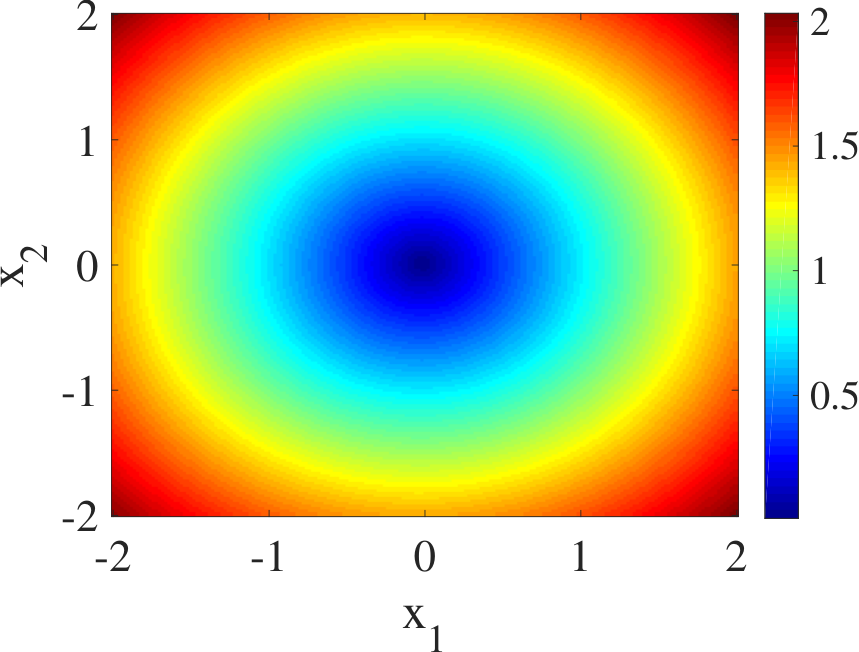
To demonstrate the effectiveness of the T-SSD algorithm in approximating Koopman eigenfunctions and invariant subspaces, we focus on the subspace identified with . In accordance with Proposition 6.6, T-SSD identifies the trivial eigenfunction spanning the maximal Koopman-invariant subspace of . T-SSD also approximates another real-valued eigenfunction with eigenvalue , whose absolute value is illustrated in Figure 2(right). Given that , this eigenfunction predicts the existence of a forward invariant set (the periodic orbit in Figure 2(left)) at its zero-level set.

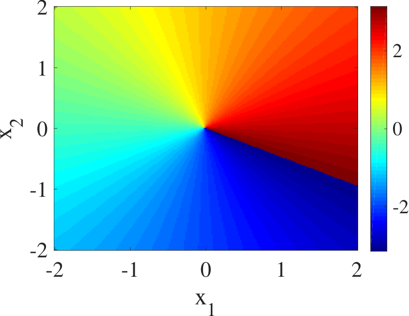
In addition, T-SSD also identifies two pairs of complex eigenfunctions. For space reasons, we only show in Figure 3 one eigenfunction with eigenvalue (the one closest to the unit circle). Its phase characterizes the oscillation of the trajectories in the state space.
To illustrate the efficacy of our algorithm regarding the prediction accuracy of the dictionary, we consider the relative linear prediction error associated with a dictionary at point given data snapshot matrices and defined by
| (41) |
where . Figure 4 compares this error on the state space for the dictionary identified by T-SSD with and for the original dictionary . This error is evaluated at points other than the training data and clearly shows the advantage of over the original dictionary both in prediction errors and capturing the radial symmetry of the vector field.


Noting that the error in (41) depends on the dictionary and does not provide information about the subspace it spans (or the individual members of the subspace), we also consider the latter. For this reason, we use the data sampling strategy used earlier to build a test data set denoted by snapshot matrices and with samples. Given a dictionary , we evaluate the invariance proximity of as the smallest such that and are -apart. This data-driven measure is equivalent to the maximum relative root mean square error for a function in the span of a given dictionary on the test data defined as
| (42) |
where and correspond to the th rows of and respectively, , and is the map defining the dynamics (9.1). The predictor is defined in (23) and calculated based on the test data. It is important to note that the evaluation of the error in (9.1) goes beyond the assumptions of Theorem 6.2, since the dictionary is identified with the original data , but the error is evaluated on the test data (instead, the guarantee of Theorem 6.2 are only valid when the error is evaluated on the original data). Following the reasoning in the proof of Theorem 6.2 and Definition 4.2, one can analytically show that
where denotes the largest eigenvalue of the argument. Table 2 shows the maximum relative root mean square error for the subspaces identified by T-SSD given different values of . According to Table 2, despite the fact that we have used different data for identification and evaluation, the error on the test data satisfies the upper bound accuracy requirement enforced by the accuracy parameter .
| 0.02 | 0.05 | 0.10 | 0.15 | 0.20 | |
|---|---|---|---|---|---|
| 0.037 | 0.100 | 0.115 | 0.185 |
9.2 Duffing System
Consider the Duffing system (Williams et al. 2015) on ,
| (43) |
with state , which has an unstable equilibrium at the origin and two asymptotically stable equilibria at and . We consider the discretized version of (9.2) with time step and gather data snapshots in matrices and from trajectories with length equal to two time steps and initial conditions uniformly selected from . Similarly to the previous example, we use a dictionary with elements spanning the space of all polynomials up to degree such that the columns of are orthonormal.
We apply the Efficient T-SSD algorithm, cf. Section 8, with . Table 3 shows the dimension of the identified dictionary, , versus the value of the design parameter . For , T-SSD identifies the original dictionary, certifying that the range spaces of and are -apart. On the other hand, the one-dimensional subspace identified by is in fact the maximal Koopman-invariant subspace of , spanned by the trivial eigenfunction with eigenvalue .
| 0.01 | 0.02 | 0.08 | 0.14 | 0.20 | 0.26 | |
|---|---|---|---|---|---|---|
| 1 | 2 | 20 | 44 | 58 | 66 |
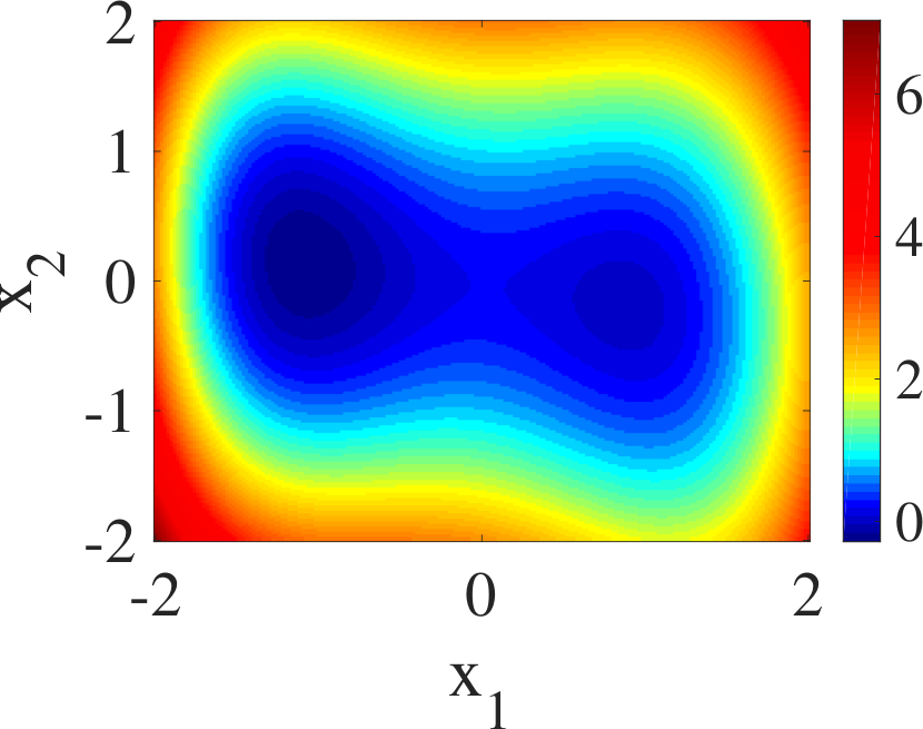
To demonstrate the effectiveness of the T-SSD algorithm in approximating Koopman eigenfunctions and invariant subspaces, we focus on the subspace identified with . Consistent with Proposition 6.6, T-SSD identifies the trivial eigenfunction spanning the maximal Koopman-invariant subspace of . T-SSD also approximates another real-valued eigenfunction with eigenvalue depicted in Figure 5(right), which clearly captures the attractiveness of the asymptotically stable equilibria and the general behavior of the vector field depicted in Figure 5(left).
To illustrate the efficacy of our algorithm regarding the prediction accuracy of the dictionary, Figure 6 compares the relative linear prediction error (41) on the state space for the dictionary identified by T-SSD with and for the original dictionary evaluated at out-of-sample points other than . Figure 6 clearly shows the effectiveness of the T-SSD algorithm in improving the prediction accuracy.


To analyze the error for individual functions in the identified subspaces by T-SSD, we form a random test data set , gathered with the same number of elements and sampling strategy used for and . Table 4 shows the maximum relative root mean square error defined in (9.1) for the subspaces identified by T-SSD given different values of . Despite the fact that we use different data for identification and evaluation, Table 4 shows the effectiveness of the T-SSD algorithm for identifying subspaces on which all functions have prediction errors characterized by the accuracy parameter .
| 0.01 | 0.02 | 0.08 | 0.14 | 0.20 | 0.26 | |
|---|---|---|---|---|---|---|
| 0.004 | 0.054 | 0.123 | 0.190 | 0.236 |
9.3 Consensus on Harmonic Mean
Given agents with state communicating through a graph with adjacency matrix , consider the dynamics
| (44) |
where is the element of on row and column and is the harmonic mean of the state elements defined as
For any initial condition , all the state elements converge to the harmonic mean of the initial condition (Cortés 2008, Proposition 10), i.e., the agents achieve consensus on . For the purpose of this example, we consider agents communicating through an undirected ring graph and states belonging to the state space . We consider the discretized version of (44) with time step and gather data snapshots in matrices and from trajectories with length equal to two time steps and initial conditions uniformly selected from . For our dictionary, we consider the space of all polynomials up to degree and choose a dictionary with functions spanning the space such that the columns of are orthonormal.
We apply the Efficient T-SSD algorithm, cf. Section 8, with . Table 5 shows the dimension of the identified dictionary, , versus the value of the design parameter . For , T-SSD identifies the original subspace, certifying that the range spaces of and are -apart. On the other hand, the one-dimensional subspace identified by is in fact the maximal Koopman-invariant subspace of , spanned by the trivial eigenfunction with eigenvalue .
| 0.05 | 0.15 | 0.30 | 0.55 | 0.80 | |
|---|---|---|---|---|---|
| 1 | 14 | 64 | 272 | 462 |
To illustrate the efficacy of T-SSD algorithm regarding prediction accuracy, we first form a test data set comprised of snapshots matrices and sampled with the same sampling strategy and number of samples as and . Figure 7 provides histogram plots comparing the relative prediction error defined in (41) of the dictionary identified by T-SSD with and the original dictionary applied on the test data. In Figure 7 the horizontal axis denotes the prediction error while the vertical axis shows the percentage of test data per interval. Figure 7 clearly shows the effectiveness of the T-SSD algorithm in improving the prediction accuracy.

We also consider the prediction accuracy for the individual functions. Table 6 shows the maximum relative root mean square error defined in (9.1) for the subspaces identified by T-SSD given different values of . According to Table 6, despite using different data for identification and evaluation, the error on the test data satisfies the upper bound accuracy requirement enforced by the accuracy parameter .
| 0.05 | 0.15 | 0.30 | 0.55 | 0.8 | |
|---|---|---|---|---|---|
| 0.144 | 0.295 | 0.549 | 0.769 |
10 Conclusions
We have presented the T-SSD algorithm, a data-driven strategy that employs data snapshots from an unknown dynamical system to refine a given dictionary of functions, yielding a subspace close to being invariant under the Koopman operator. A design parameter allows to balance the prediction accuracy and expressiveness of the algorithms’ output, which always contains the maximal Koopman-invariant subspace and all Koopman eigenfunctions in the span of the original dictionary. The proposed algorithm generalizes both Extended Dynamic Mode Decomposition and Symmetric Subspace Decomposition. Future work will investigate noise-resilient strategies to approximate Koopman-invariant subspaces and methods to construct expressive dictionaries with high accuracy by alternating between growing the set of functions (using specific basic functions or neural networks) and pruning the dictionary to enhance accuracy while providing accuracy bounds for all members of the identified vector space of functions. Moreover, we aim to explore the application of the proposed method in stability analysis, data-driven construction of Lyapunov functions66 6 The recent work (Mamakoukas et al. 2022, Section V.C) provides an interesting example of using the T-SSD algorithm as a subroutine precisely for this purpose., and designing control schemes with formal performance and stability guarantees by using the Koopman operator to model control systems as bilinear or switched-linear systems.
References
- Absil et al. (2009) P. A. Absil, R. Mahony, and R. Sepulchre. Optimization algorithms on matrix manifolds. Princeton University Press, 2009.
- Anderson Jr et al. (1985) W. N. Anderson Jr, E. J. Harner, and G. E. Trapp. Eigenvalues of the difference and product of projections. Linear and Multilinear Algebra, 17(3-4):295–299, 1985.
- Brunton et al. (2016a) S. L. Brunton, B. W. Brunton, J. L. Proctor, and J. N. Kutz. Koopman invariant subspaces and finite linear representations of nonlinear dynamical systems for control. PLOS One, 11(2):1–19, 2016a.
- Brunton et al. (2016b) S. L. Brunton, J. L. Proctor, and J. N. Kutz. Discovering governing equations from data by sparse identification of nonlinear dynamical systems. Proceedings of the National Academy of Sciences, 113(15):3932–3937, 2016b.
- Budišić et al. (2012) M. Budišić, R. Mohr, and I. Mezić. Applied Koopmanism. Chaos, 22(4):047510, 2012.
- Choi et al. (2020) H. Choi, U. Vaidya, and Y. Chen. A convex data-driven approach for nonlinear control synthesis. arXiv preprint arXiv:2006.15477, 2020.
- Cortés (2008) J. Cortés. Distributed algorithms for reaching consensus on general functions. Automatica, 44(3):726–737, 2008.
- Dawson et al. (2016) S. T. M. Dawson, M. S. Hemati, M. O. Williams, and C. W. Rowley. Characterizing and correcting for the effect of sensor noise in the dynamic mode decomposition. Experiments in Fluids, 57(3):42, 2016.
- Folkestad et al. (2020) C. Folkestad, Y. Chen, A. D. Ames, and J. W. Burdick. Data-driven safety-critical control: Synthesizing control barrier functions with Koopman operators. IEEE Control Systems Letters, 5(6):2012–2017, 2020.
- Goswami and Paley (2022) D. Goswami and D. A. Paley. Bilinearization, reachability, and optimal control of control-affine nonlinear systems: A Koopman spectral approach. IEEE Transactions on Automatic Control, 67(6):2715–2728, 2022.
- Haseli and Cortés (2019) M. Haseli and J. Cortés. Approximating the Koopman operator using noisy data: noise-resilient extended dynamic mode decomposition. In American Control Conference, pages 5499–5504, Philadelphia, PA, July 2019.
- Haseli and Cortés (2021a) M. Haseli and J. Cortés. Data-driven approximation of Koopman-invariant subspaces with tunable accuracy. In American Control Conference, pages 469–474, New Orleans, LA, July 2021a.
- Haseli and Cortés (2021b) M. Haseli and J. Cortés. Parallel learning of Koopman eigenfunctions and invariant subspaces for accurate long-term prediction. IEEE Transactions on Control of Network Systems, 8(4):1833–1845, 2021b.
- Haseli and Cortés (2022) M. Haseli and J. Cortés. Learning Koopman eigenfunctions and invariant subspaces from data: Symmetric Subspace Decomposition. IEEE Transactions on Automatic Control, 67(7):3442–3457, 2022.
- Johnson and Yeung (2018) C. A. Johnson and E. Yeung. A class of logistic functions for approximating state-inclusive Koopman operators. In American Control Conference, pages 4803–4810, Milwaukee, WI, June 2018. IEEE.
- Kaiser et al. (2021) E. Kaiser, J. N. Kutz, and S. L. Brunton. Data-driven discovery of Koopman eigenfunctions for control. Machine Learning: Science and Technology, 2(3):035023, 2021.
- Klus et al. (2016) S. Klus, P. Koltai, and C. Schütte. On the numerical approximation of the Perron-Frobenius and Koopman operator. Journal of Computational Dynamics, 3(1):51–79, 2016.
- Klus et al. (2020) S. Klus, F. Nüske, S. Peitz, J. H. Niemann, C. Clementi, and C. Schütte. Data-driven approximation of the Koopman generator: Model reduction, system identification, and control. Physica D: Nonlinear Phenomena, 406:132416, 2020.
- Koopman (1931) B. O. Koopman. Hamiltonian systems and transformation in Hilbert space. Proceedings of the National Academy of Sciences, 17(5):315–318, 1931.
- Koopman and Neumann (1932) B. O. Koopman and J. V. Neumann. Dynamical systems of continuous spectra. Proceedings of the National Academy of Sciences, 18(3):255–263, 1932.
- Korda and Mezić (2018a) M. Korda and I. Mezić. Linear predictors for nonlinear dynamical systems: Koopman operator meets model predictive control. Automatica, 93:149–160, 2018a.
- Korda and Mezić (2018b) M. Korda and I. Mezić. On convergence of extended dynamic mode decomposition to the Koopman operator. Journal of Nonlinear Science, 28(2):687–710, 2018b.
- Korda and Mezic (2020) M. Korda and I. Mezic. Optimal construction of Koopman eigenfunctions for prediction and control. IEEE Transactions on Automatic Control, 65(12):5114–5129, 2020.
- Lu and Tartakovsky (2020) H. Lu and D. M. Tartakovsky. Prediction accuracy of dynamic mode decomposition. SIAM Journal on Scientific Computing, 42(3):A1639–A1662, 2020.
- Lusch et al. (2018) B. Lusch, J. N. Kutz, and S. L. Brunton. Deep learning for universal linear embeddings of nonlinear dynamics. Nature Communications, 9(1):1–10, 2018.
- Mamakoukas et al. (2019) G. Mamakoukas, M. Castano, X. Tan, and T. Murphey. Local Koopman operators for data-driven control of robotic systems. In Robotics: Science and Systems, Freiburg, Germany, June 2019.
- Mamakoukas et al. (2021) G. Mamakoukas, M. L. Castano, X. Tan, and T. D. Murphey. Derivative-based Koopman operators for real-time control of robotic systems. IEEE Transactions on Robotics, 2021.
- Mamakoukas et al. (2022) G. Mamakoukas, I. Abraham, and T. D. Murphey. Learning stable models for prediction and control. https://arxiv.org/abs/2005.04291v2, 2022.
- Marsden and McCracken (2012) J. E. Marsden and M. McCracken. The Hopf bifurcation and its applications, volume 19. Springer Science & Business Media, 2012.
- Mauroy and Mezić (2016) A. Mauroy and I. Mezić. Global stability analysis using the eigenfunctions of the Koopman operator. IEEE Transactions on Automatic Control, 61(11):3356–3369, 2016.
- Mezić (2005) I. Mezić. Spectral properties of dynamical systems, model reduction and decompositions. Nonlinear Dynamics, 41(1-3):309–325, 2005.
- Nüske et al. (2021) F. Nüske, S. Peitz, F. Philipp, M. Schaller, and K. Worthmann. Finite-data error bounds for Koopman-based prediction and control. arXiv preprint arXiv:2108.07102, 2021.
- Otto and Rowley (2019) S. E. Otto and C. W. Rowley. Linearly recurrent autoencoder networks for learning dynamics. SIAM Journal on Applied Dynamical Systems, 18(1):558–593, 2019.
- Pan et al. (2021) S. Pan, N. Arnold-Medabalimi, and K. Duraisamy. Sparsity-promoting algorithms for the discovery of informative Koopman-invariant subspaces. Journal of Fluid Mechanics, 917, 2021.
- Peitz and Klus (2019) S. Peitz and S. Klus. Koopman operator-based model reduction for switched-system control of PDEs. Automatica, 106:184–191, 2019.
- Rowley et al. (2009) C. W. Rowley, I. Mezić, S. Bagheri, P. Schlatter, and D. S. Henningson. Spectral analysis of nonlinear flows. Journal of Fluid Mechanics, 641:115–127, 2009.
- Schmid (2010) P. J. Schmid. Dynamic mode decomposition of numerical and experimental data. Journal of Fluid Mechanics, 656:5–28, 2010.
- Son et al. (2020) S. H. Son, A. Narasingam, and J. S. Kwon. Handling plant-model mismatch in Koopman Lyapunov-based model predictive control via offset-free control framework. arXiv preprint arXiv:2010.07239, 2020.
- Takeishi et al. (2017) N. Takeishi, Y. Kawahara, and T. Yairi. Learning Koopman invariant subspaces for dynamic mode decomposition. In Conference on Neural Information Processing Systems, pages 1130–1140, 2017.
- Trefethen and Bau (1997) L. N. Trefethen and D. Bau. Numerical Linear Algebra. SIAM, Philadelphia, PA, 1997.
- Tu et al. (2014) J. H. Tu, C. W. Rowley, D. M. Luchtenburg, S. L. Brunton, and J. N. Kutz. On dynamic mode decomposition: theory and applications. Journal of Computational Dynamics, 1(2):391–421, 2014.
- Williams et al. (2015) M. O. Williams, I. G. Kevrekidis, and C. W. Rowley. A data-driven approximation of the Koopman operator: Extending dynamic mode decomposition. Journal of Nonlinear Science, 25(6):1307–1346, 2015.
- Yeung et al. (2019) E. Yeung, S. Kundu, and N. Hodas. Learning deep neural network representations for Koopman operators of nonlinear dynamical systems. In American Control Conference, pages 4832–4839, Philadelphia, PA, July 2019.
- Zhang and Zuazua (2021) C. Zhang and E. Zuazua. A quantitative analysis of Koopman operator methods for system identification and predictions. https://hal.archives-ouvertes.fr/hal-03278445, 2021.
- Zinage and Bakolas (2022) V. Zinage and E. Bakolas. Koopman operator based modeling for quadrotor control on SE(3). IEEE Control Systems Letters, 6:752–757, 2022.
Appendix A Basic Algebraic Results
Here we collect two algebraic results from (Haseli and Cortés 2022) that are used in our technical treatment.
Lemma A.1
((Haseli and Cortés 2022, Lemma A.1)): Let be matrices with full column rank. Suppose that the columns of form a basis for the null space of , where . Then,
- a.
;
- b.
and have full column rank.
Lemma A.2
((Haseli and Cortés 2022, Lemma A.2)): Let be matrices of appropriate sizes, with having full column rank. Then if and only if .