https://doi.org/10.1016/j.jeconom.2021.07.002
Journal of Econometrics, accepted manuscript.
Fully Modified Least Squares Cointegrating Parameter Estimation in
Multicointegrated Systems
© 2021 This manuscript version is made available under the CC-BY-NC-ND 4.0 license
https://creativecommons.org/licenses/by-nc-nd/4.0/
bCenter for Econometrics and Business Analytics, St. Petersburg State University, Russia
cYale University, USA
dUniversity of Auckland, New Zealand
eUniversity of Southampton, UK
fSingapore Management University, Singapore
August 11, 2026
Abstract
Multicointegration is traditionally defined as a particular long run relationship among variables in a parametric vector autoregressive model that introduces additional cointegrating links between these variables and partial sums of the equilibrium errors. This paper departs from the parametric model, using a semiparametric formulation that reveals the explicit role that singularity of the long run conditional covariance matrix plays in determining multicointegration. The semiparametric framework has the advantage that short run dynamics do not need to be modeled and estimation by standard techniques such as fully modified least squares (FM-OLS) on the original system is straightforward. The paper derives FM-OLS limit theory in the multicointegrated setting, showing how faster rates of convergence are achieved in the direction of singularity and that the limit distribution depends on the distribution of the conditional one-sided long run covariance estimator used in FM-OLS estimation. Wald tests of restrictions on the regression coefficients have nonstandard limit theory which depends on nuisance parameters in general. The usual tests are shown to be conservative when the restrictions are isolated to the directions of singularity and, under certain conditions, are invariant to singularity otherwise. Simulations show that approximations derived in the paper work well in finite samples. The findings are illustrated empirically in an analysis of fiscal sustainability of the US government over the post-war period.
Keywords: Cointegration, Multicointegration, Fully modified regression, Singular long run variance matrix, Degenerate Wald test, Fiscal sustainability.
JEL Codes: C12, C13, C22
1 Introduction
Many economic time series are non-stationary and contain stochastic trends, which are naturally modeled using cointegration. For example, two variables and are cointegrated if for some , is . Granger and Lee (1990) call multicointegration a situation when the cumulative error is cointegrated with or . They analyze a case where are production, sales and inventory investment, and is the level of inventories. Inventory stock may then be cointegrated with production via an adjustment mechanism that captures firm decision making on inventory investment, as well as satisfying an identity arising from the aggregation of the defining relationship .
It is important to take into account the presence of multicointegration in a cointegrated system: on one hand it can invalidate usual procedures of estimation and testing in cointegrated systems by affecting asymptotic properties; and on the other it may lead to advantages in improved forecasting performance. Multicointegration has so far been analyzed only in a VAR framework11 1 It is of course possible to write stationary VARs in moving average form and vice versa under invertibility conditions. There is now a large literature describing such explicit representations for cointegrated time series. For a general approach based of Laurent series representations, see Franchi and Paruolo (2019) and the references therein. and naturally involves implicit restrictions on the model induced by the extra layer of cointegration. Engsted and Johansen (1999), for example, show that if the process is generated by a VAR model for variables, multicointegration may occur if but not if . Likelihood-based estimators of cointegration parameters in VAR multicointegrated systems have mixed normal limit distributions and likelihood ratio statistics for hypothesis testing about the parameters generally have asymptotic null distributions under conditions of correct specification, as shown for example in Johansen (1997, 2006), Boswijk (2000, 2010), and Paruolo (2000). Berenguer-Rico and Carrion-i-Silvestre (2011) provide an application of this approach that examines government debt sustainability.
In contrast to these studies, the present paper studies cointegrated models that are possibly multicointegrated in a semiparametric framework with specific focus on the use of fully modified least squares (FM-OLS) estimation. In related work, the authors (Phillips and Kheifets, 2019) explore the concept of multicointegration in a general triangular cointegrated system with weakly dependent errors, showing how multicointegration emerges naturally from singularity of the long run covariance matrix. This formulation gives an explicit mechanism generating multicointegration as a property of a general triangular system, as opposed to imposing multicointegration subsequently on a parametric system like a VAR. The contrast lies in the capacity of a general I(1) triangular system to implicitly involve the effects of multicointegration without changing or restricting the cointegrating coefficients. The implicit effects propagate from the nonparametric treatment of the equation errors and are therefore typically unknown to the investigator. This property is one of the primary motivations of our study. A second motivation is to show that FM-OLS estimation of the cointegration coefficients has some useful robustness properties to the possible unknown presence of multicointegration.
More specifically, the present paper contributes by developing asymptotic theory for FM-OLS estimation and testing in cointegrating relationships that involve multicointegration in a semiparametric setting. The analysis of triangular cointegrated systems under singularity that is developed is of some independent interest. The results show that cointegrated system estimation may proceed under certain conditions in a general cointegrated system in the presence (and without prior knowledge) of multicointegration.
To define multicointegration for weakly dependent data, we take the triangular representation of a linear cointegrating relationship. In the cointegrating regression model
| (1) |
is a cointegrating coefficient matrix, is initialized at by , and the combined error vector follows the linear process
| (2) |
for some , finite fourth order cumulants of , and where . It is common in the literature to consider such time series with an additional assumption (e.g. Phillips, 1995) that assures nonsingularity of the long run variance matrix of , which we relax here.
Let . The linear operator , the long run covariance matrix of and one-sided long run covariance matrix of are partitioned conformably with as
where is positive definite so that is a full rank regressor vector, as commonly assumed in triangular systems such (1) and (2) following Phillips(1991)22 2 The case where the regressors are themselves cointegrated is considered in Phillips (1995) but is not considered in this paper.. The conditional long run covariance matrix, defined as the Schur complement of the block , is and is positive (semi-) definite if and only if is positive (semi-) definite (by virtue of the Guttman rank additivity formula). In this paper we consider a situation when the long run variance matrix is singular, or, equivalently, when the conditional long run covariance matrix is singular. It corresponds to a case where partial sums of and are cointegrated with an error in some unknown direction, i.e. when there is a multicointegration in the spirit of Granger and Lee (1990), but is semiparametric in the sense that the short run dynamics are left unspecified. We therefore introduce the following definition.
Definition 1.
The process generated by a triangular cointegrating system is called multicointegrated if its long run error covariance matrix is singular.
The advantage of this framework is that it provides the explicit origin from which the multicointegrating relationship arises in an system. Thus, if we take partial sums of the augmented regression form (Phillips, 1991)
| (3) |
where is the long run regression coefficient of on and , giving (using capitals with time index for partial sums)
| (4) |
It becomes clear that in the direction of singularity of we have an exact long run relationship that links the time series , , and and this relationship is prescribed in terms of the coefficients , and the singular direction of , which is estimable. In earlier work on multicointegration, the hypothesis about multicointegration is imposed a priori, directly and explicitly as in Granger and Lee (1990) or through rank conditions in VAR analyses. What our approach does is: (i) show that multicointegration may exist in a triangular system such as (1); (ii) reveal the leading and intuitively simple role that the singularity of the long run conditional error covariance matrix plays in giving rise to multicointegration, a feature of the model that may be unknown to the investigator; (iii) allow for both cointegration and multicointegration within the same specification; and (iv) use a nonparametric formulation to provide a general setting for the analysis, for the form of the cointegrating and multicointegrating coefficients, and for practical work.
In a VAR framework Engsted and Johansen (1999) show that multicointegration, as defined in Granger and Lee (1990) of a linear process33 3 The summability condition in the specification (2) imposes a restriction on . This is because the matrix moving average power series of a linear process generated by (1)-(2) does not have poles at , which implies that, when the system is written in the form , it must be that , where . Indeed, the upper block of of such a system satisfies and does not have poles at if and only if . We thank a referee for this clarifying observation and suggestions to improve the statement and the proof of Proposition 1. where the roots of satisfy or , occurs when is a root44 4 The order of zeros of at or, equivalently, the order of poles of at , is not restricted to and is unknown. A unified treatment of the different representations of cointegrated systems for known is given in a recent paper by Franchi and Paruolo (2019)., so that has reduced rank and is singular (explicit forms of the matrices and their orthogonal complements are given in the proof of the Proposition 1). This is the case when is singular or more specifically in the present context when is singular, as shown below.
Proposition 1.
In what follows data matrices are denoted by upper case letters without indexes, e.g., . The OLS estimator is consistent at the rate at least . The FM-OLS estimator (Phillips and Hansen 1990) has the form and employs corrections for endogeneity in the regressor , leading to the transformed dependent variable and a bias correction term involving , which is constructed in the usual way using consistent nonparametric estimators of submatrices of the long run and one sided long run quantities and . Compared with OLS, the FM-OLS estimator removes asymptotic bias and increases efficiency by correcting both the long run serial correlation in and endogeneity in caused by the long run correlation between and . The properties of FM-OLS in general regressions as well as VARs are studied in Phillips (1995). Here we advance the analysis by allowing for the possibility of a singular conditional long run variance matrix . When is singular, i.e. when modified is cointegrated and in some direction the errors in the cointegrating equation are , the limit theory of the FM-OLS estimator is degenerate at the usual rate and the faster convergence rate affects both estimation and inference.
The paper makes the following contributions. First, we derive the new rates of convergence and limit distribution of the FM-OLS estimator in the case of a null conditional long run variance matrix. The new rate exceeds and depends on the bandwidth used in estimating the long run covariance matrix quantities that are employed in making corrections for endogeneity and serial correlation in FM-OLS. The resulting limit distribution is no longer mixed normal and depends on nuisance parameters. Similar properties hold in the direction of singularity in the case of a singular long run variance matrix. Second, under certain conditions, the limit distribution of Wald statistics for testing restrictions on the cointegrating space and cointegrating parameters is and is invariant to the presence of singularity. Third, we show that when those restrictions fail, the Wald test is conservative. Monte Carlo simulations reveal that the empirical level of the test can be far below the nominal , and levels in singular and near singular cases.
As an application of our methods we analyze fiscal sustainability of the US government over the period 1947-2019 by testing the null hypothesis that the cointegration relationship between government revenue and expenditure has the parametric form . Multicointegration between government revenue and expenditure naturally arises if bounds are imposed on deviations of debt from revenue. We reject the null hypothesis and, as our theoretical results show, this conclusion is not affected by the presence of multicointegration. The finding is important for practical purposes, as a separate treatment of the multicointegration case is not necessary (cf., Quintos, 1995, and Berenguer-Rico and Carrion-i-Silvestre, 2011).
The paper is organized as follows. In Section 2 we derive the rates of convergence of elements of and establish its limit distribution. After some preliminary observations we begin our discussion with the null case where , then move on to a case of a general singular matrix. The implications of singularity for hypothesis testing are discussed in Section 3. The finite sample properties of the FM-OLS and Wald test statistics are explored in Section 4. The application to government fiscal sustainability is considered in Section 5. Section 6 concludes. Proofs are given in the Appendix.
2 Fully Modified OLS
Under the stated conditions the functional law holds for partial sums of (e.g., Phillips and Solo, 1992). Define the partition into the first and the final subvectors of the Brownian motion, conformably with . Introducing the matrices
and the Brownian motion , we have
where is orthogonal to . Note that is the long run variance of , where . It is well known that the OLS estimator of in (1) is consistent with a limit distribution that depends on the nuisance parameters and , viz.,
| (5) |
The last two terms of (2) are the endogeneity and serial correlation biases that FM-OLS seeks to remove.
Suppose and are estimated in the usual way (e.g., Priestley 1981; Hannan, 1970) as
where is a kernel function, is a bandwidth parameter and the sample covariances are , where . Similar to Phillips (1995), we consider the following kernels and bandwidth rates.
Assumption K (Kernel Condition) For given , the bandwidth parameter has the rate as , where is slowly varying at infinity, i.e. for and . The kernel function is a twice continuously differentiable even function with
- (a)
, and
- (b)
, with .
Parzen and Tukey–Hanning kernels satisfy Assumption K. The Bartlett–Priestley or quadratic spectral kernels do not satisfy Assumption K but to use them in the following development these kernels need to satisfy
- (b’)
, as
and (a) with support . Under Assumption K, with , and any consistent estimator we have
Proposition 2.
Under Assumption K with ,
For the nonsingular case this result appears in Corollary 4.3 in Phillips (1995). The proof reveals that singularity does not alter the above convergence but makes the limit distribution degenerate. If has full rank, the rate of convergence of the FM-OLS estimator is determined by the rates of weak convergence of the sample covariances and the rate of nonparametric estimation of and does not play any role. We will show that in case is singular, the rate of convergence of the FM-OLS estimator along the null direction of increases by , where
The fastest rate of convergence of FM-OLS in the null direction is when bandwidth expansion rate is .
For example, in the case where , we have and the precise rate of convergence of the FM-OLS estimator depends on the bandwidth parameter expansion rate in kernel estimation of the nonparametric components. Parameter dependencies may then be present in the resulting asymptotic theory, arising from first order terms in the limit behavior of the long run covariances that influence the asymptotics in this degenerate case. In particular, when the component in the Beveridge-Nelson decomposition of . In this case, reduces to a first difference , which is 55 5 The fact that is includes the possibility that in some or all directions may be , , but that possibility does not affect the convergence properties of the FM-OLS estimator as the next proposition shows. with , with , and has long run variance matrix .
The next proposition establishes convergence properties of FM-OLS for such time series. It is particularly useful for the case of a single cointegration relationship with (e.g., Phillips and Loretan, 1991), because singularity implies that the conditional long run variance is zero. This reduction makes explicit the effect of singularity on the convergence rates and serves as the basis of a general result.
Proposition 3.
Suppose . Under Assumption K with ,
As the proof of Proposition 3 reveals, the limit distribution of the restandardized estimation error depends on nuisance parameters associated with the nonparametric estimation of the long run covariance matrices. For kernel estimators, the limit depends on the covariance structure of the errors, on the bandwidth growth rate, and on the second derivative of the kernel function. For illustration, consider the case when the bandwidth grows slower than , which includes the typical optimal bandwidth rate for long run variance estimation. Under these conditions, we have the following limit theory.
Proposition 4.
Suppose . Under Assumption K with ,
where .
Unlike the corresponding limit theory in the nonsingular case (Phillips, 1995; Phillips and Hansen, 1990; Phillips, 2014), the limit distribution of FM-OLS now depends on the covariance structure of the errors and and on the second derivative of the kernel function.
Next, consider a general case of singular with rank , so that has rank . To isolate nondegenerate directions decompose , where is an matrix of rank . Then has full rank, has full rank long run variance matrix and Proposition 2 applies in this direction. In the orthogonal direction66 6 By the usual eigenvalue decomposition for symmetric matrices there is a set of orthonormal eigenvectors of , stacked as an orthogonal matrix and real eigenvalues in decreasing order on diagonal matrix , such that . In this notation, and spans the space of eigenvectors corresponding to zero eigenvalues. , is 77 7 This representation allows for being with in some directions., where has long run variance and Proposition 3 applies, showing that elements in this direction are estimated at a faster rate than .
We now state our first main result.
Theorem 1.
Suppose , where is an matrix with . Then under Assumption K
which is degenerate mixed normal. The limit distribution is not degenerate and has full rank in direction with
where and is the full rank conditional long run variance matrix of . In the direction orthogonal to the convergence of is at the faster rate and
The FM-OLS estimator of a singular triangular system with multicointegration therefore has the following properties: (i) FM-OLS is consistent; (ii) the limit distribution is degenerate in the original coordinates; and (iii) rates of convergence are in nondegenerate directions and in degenerate directions. In the degenerate direction the limit distribution is of the type shown in Proposition 4. Singularity of the limit distribution means that care is needed when undertaking inference and these matters are considered in the next section. The situation is in some ways analogous to that of causality testing in cointegrated VAR regressions, as analyzed in Toda and Phillips (1993), and cointegrating regressions with cointegrated regressors, as analyzed in Phillips (1995). In the present case, it is necessary to analyze the directions of singularity of the long run covariance structure and the behavior of the estimates in these directions.
3 Testing
We consider the following hypothesis involving functions , the space of dimensional continuously differentiable functions where is row vectorization. Suppose , where is an matrix of , so that is nonsingular. Then under Assumption K
The limit distribution is mixed normal () and standard inference methods can be applied. The usual Wald statistic for testing is
where , and is row vectorization. Suppose that the following rank condition holds
| (6) |
Under Assumption K, . So, under the rank condition (6), the limit distribution of the Wald statistics is invariant to the presence of singularity.
3.1 Violation of the rank condition
Consider the linear hypothesis
with restriction matrix of rank and component matrices , , of rank and , , of rank . Then has a tensor form with matrix representation , and
If the rank of is , then the rank condition (6) fails as . This is the case where some of the restrictions isolate directions in which FM-OLS is hyperconsistent with rate exceeding . The distribution of the Wald test statistic is then nonstandard and depends on nuisance parameters. In general, failure of estimator mixed normality in the direction of faster convergence produces a non chi-squared limit in the Wald statistic as the faster convergence of the estimator is balanced in the Wald statistic weighting. A related phenomenon arises in Toda and Phillips (1993), who describe situations where Wald tests of Granger causality in cointegrated VAR systems do not follow asymptotically chi-squared distributions. For another example, see Phillips (2016), where singularity in the signal matrix leads to nonstandard inference.
To illustrate the consequences of singularity consider testing Then and their ranks are , and . The Wald test statistic then simplifies to
The notational change to emphasizes that the following analysis only considers the full dimensional restriction structures above. The rank of equals the rank of the conditional long run variance times , i.e. the null hypothesis restrictions isolate ‘all directions’ and the rank condition is satisfied if and only if the conditional long run variance matrix is nonsingular. If the conditional long run variance is nonsingular, the rank condition holds and .
Singularity alters the rate of convergence and the limit of , which is used in the construction of the Wald test statistics. We proceed to derive the rate of convergence for this quantity. As the proof of the following proposition reveals, the rate of convergence is if and if . As in the case of FM-OLS estimation, the limit distribution of depends on nuisance parameters and on the implementation of the nonparametric estimates of the long run covariance matrices. As an illustration, consider a case when the bandwidth grows slower than , which includes the usual optimal bandwidth rate for long run variance estimation.
Proposition 5.
Suppose and Assumption K holds with .Then
- (a)
- (b)
If is nonsingular, then if and if .
Nonsingularity of means that there is no further level of cointegration (system (1) is singular of first order, see Park 1992) and guarantees that the limit in Part (a) is nondegenerate, so that the rate of convergence of is sharp. In the more general case where is positive semi-definite but not a null matrix we have the following result.
Theorem 2.
Suppose , where is an matrix with , is nonsingular, and Assumption K holds with , then under the null .
The proof of the above result reveals that the limit distribution of the Wald test statistic involves the sum of two major components. The first component arises from the limit in the nonsingular direction, which is , and the second involves the limit in the direction where the conditional long run variance matrix is zero, which is nonstandard, depends on nuisance parameters and decays at the speed established in Proposition 5 above. Therefore, for the limit distribution of the statistic has thinner tails than the distribution of , so that tests based on the usual degrees of freedom are asymptotically conservative.
4 Finite sample performance
The following analysis of finite sample performance is based on simulations with different sample sizes.88 8 Statistical computing in this paper uses R version 3.4.4. The long run variances are estimated using the Parzen kernel
and bandwidth is set to , if not specified otherwise. The data generating process (DGP) has the form (1) with scalar cointegrating coefficient and with a combined error vector that follows the linear process
We consider estimation of and hypothesis testing for the null . We look at two classes of bivariate () DGPs.
- DGP1
For parameter choices define
- DGP2
For parameter choices define


The finite sample performance for DGP1 is shown in Figure 1 and Table 1; results for DGP2 are given in Figure 2 and Table 2.
Discussion of results for DGP1.
When we have and a singular system. The limit theory generalizes results on estimation and testing to this case. With matrix diagonal, the errors and are independent and the effect of singularity in the long run variance can be studied separately from the effect of long run dependence. When , the long run variance is the identity and the conditional long run variance is , giving a standard nonsingular case. For values of between and the system is still in the nonsingular case but in finite samples for smaller values of the limit theory for the singular case may lead to better approximations than the nonsingular case and simulations help to guide this assessment.
In Figure 1, Panel (a), the densities of the bias are shown for sample size . We compare the densities in the singular case () with two nonsingular cases ( and ). The figure shows that the bias in the singular case is much smaller than the bias in the nonsingular cases. A more pronounced effect is observed for in Panel (c) confirming the higher convergence rates established for FM-OLS under singularity.
We use the -statistic for testing the hypothesis . In Figure 1, Panel (b) the densities of the -statistic are shown for sample size . We compare the densities in the singular case () with two nonsingular cases ( and ). Theory predicts that in nonsingular cases the test statistics is asymptotically standard normal, whose density is also plotted. This approximation is quite accurate for . However, the density of the test statistic for has thinner tails, so that the test based on standard normal approximation is conservative as our theory predicts for singular case. Results for the sample size are plotted in Panel (d), and it is evident that the test statistic for still has thin tails.
| Bias-OLS | SD-OLS | Bias | SD | t-Bias | t-SD | 0.10 | 0.05 | 0.01 | ||||
|---|---|---|---|---|---|---|---|---|---|---|---|---|
| 1 | 50 | -1.0 | 2 | 0.0001 | 0.0238 | 0.0003 | 0.0175 | 0.0044 | 0.2598 | 0.000 | 0.000 | 0.000 |
| 2 | 100 | -1.0 | 3 | -0.0001 | 0.0088 | -0.0000 | 0.0055 | -0.0023 | 0.2124 | 0.000 | 0.000 | 0.000 |
| 3 | 50 | -0.9 | 2 | 0.0000 | 0.0231 | 0.0003 | 0.0173 | 0.0047 | 0.2752 | 0.000 | 0.000 | 0.000 |
| 4 | 100 | -0.9 | 3 | -0.0001 | 0.0087 | -0.0001 | 0.0057 | -0.0031 | 0.2379 | 0.000 | 0.000 | 0.000 |
| 5 | 50 | -0.8 | 2 | -0.0000 | 0.0234 | 0.0002 | 0.0186 | 0.0050 | 0.3214 | 0.000 | 0.000 | 0.000 |
| 6 | 100 | -0.8 | 3 | -0.0001 | 0.0091 | -0.0001 | 0.0068 | -0.0041 | 0.3108 | 0.000 | 0.000 | 0.000 |
| 7 | 50 | -0.7 | 2 | -0.0001 | 0.0247 | 0.0001 | 0.0210 | 0.0053 | 0.3937 | 0.000 | 0.000 | 0.000 |
| 8 | 100 | -0.7 | 3 | -0.0001 | 0.0101 | -0.0001 | 0.0085 | -0.0050 | 0.4112 | 0.000 | 0.000 | 0.000 |
| 9 | 50 | -0.6 | 2 | -0.0001 | 0.0267 | 0.0001 | 0.0242 | 0.0056 | 0.4846 | 0.001 | 0.000 | 0.000 |
| 10 | 100 | -0.6 | 3 | -0.0001 | 0.0115 | -0.0001 | 0.0105 | -0.0059 | 0.5232 | 0.002 | 0.000 | 0.000 |
| 11 | 50 | -0.5 | 2 | -0.0002 | 0.0294 | 0.0000 | 0.0280 | 0.0060 | 0.5875 | 0.007 | 0.002 | 0.000 |
| 12 | 100 | -0.5 | 3 | -0.0001 | 0.0132 | -0.0001 | 0.0126 | -0.0068 | 0.6363 | 0.010 | 0.003 | 0.000 |
| 13 | 50 | -0.4 | 2 | -0.0003 | 0.0326 | -0.0001 | 0.0321 | 0.0063 | 0.6967 | 0.019 | 0.007 | 0.000 |
| 14 | 100 | -0.4 | 3 | -0.0001 | 0.0151 | -0.0001 | 0.0149 | -0.0077 | 0.7433 | 0.027 | 0.009 | 0.001 |
| 15 | 50 | -0.3 | 2 | -0.0003 | 0.0361 | -0.0001 | 0.0364 | 0.0066 | 0.8073 | 0.041 | 0.017 | 0.003 |
| 16 | 100 | -0.3 | 3 | -0.0001 | 0.0172 | -0.0001 | 0.0171 | -0.0084 | 0.8392 | 0.050 | 0.019 | 0.002 |
| 17 | 50 | -0.2 | 2 | -0.0004 | 0.0399 | -0.0002 | 0.0409 | 0.0069 | 0.9146 | 0.071 | 0.031 | 0.007 |
| 18 | 100 | -0.2 | 3 | -0.0001 | 0.0192 | -0.0001 | 0.0195 | -0.0090 | 0.9215 | 0.075 | 0.034 | 0.006 |
| 19 | 50 | -0.1 | 2 | -0.0005 | 0.0439 | -0.0003 | 0.0455 | 0.0071 | 1.0146 | 0.106 | 0.053 | 0.013 |
| 20 | 100 | -0.1 | 3 | -0.0001 | 0.0214 | -0.0001 | 0.0218 | -0.0094 | 0.9894 | 0.097 | 0.049 | 0.009 |
| 21 | 50 | 0.0 | 2 | -0.0005 | 0.0481 | -0.0003 | 0.0502 | 0.0073 | 1.1043 | 0.134 | 0.073 | 0.021 |
| 22 | 100 | 0.0 | 3 | -0.0002 | 0.0236 | -0.0001 | 0.0242 | -0.0098 | 1.0438 | 0.116 | 0.061 | 0.014 |
| Bias-OLS | SD-OLS | Bias | SD | t-Bias | t-SD | 0.10 | 0.05 | 0.01 | ||||
|---|---|---|---|---|---|---|---|---|---|---|---|---|
| 1 | 50 | 0.8 | 3 | 0.0207 | 0.0223 | 0.0013 | 0.0184 | 0.1368 | 1.0091 | 0.102 | 0.054 | 0.014 |
| 2 | 50 | 5.2 | 3 | 0.0026 | 0.0054 | -0.0011 | 0.0040 | -0.0442 | 0.6474 | 0.018 | 0.009 | 0.003 |
| 3 | 50 | 0.8 | 5 | 0.0207 | 0.0223 | 0.0039 | 0.0189 | 0.2638 | 1.0806 | 0.135 | 0.078 | 0.023 |
| 4 | 50 | 5.2 | 5 | 0.0026 | 0.0054 | 0.0003 | 0.0029 | 0.1242 | 0.6440 | 0.026 | 0.014 | 0.004 |
| 5 | 50 | 0.8 | 7 | 0.0207 | 0.0223 | 0.0056 | 0.0197 | 0.3659 | 1.1444 | 0.161 | 0.100 | 0.035 |
| 6 | 50 | 5.2 | 7 | 0.0026 | 0.0054 | 0.0008 | 0.0029 | 0.2425 | 0.7146 | 0.044 | 0.025 | 0.008 |
| 7 | 50 | 0.8 | 10 | 0.0207 | 0.0223 | 0.0076 | 0.0206 | 0.4959 | 1.2321 | 0.195 | 0.130 | 0.055 |
| 8 | 50 | 5.2 | 10 | 0.0026 | 0.0054 | 0.0012 | 0.0031 | 0.3657 | 0.8392 | 0.074 | 0.045 | 0.018 |
| 9 | 100 | 0.8 | 3 | 0.0104 | 0.0111 | -0.0003 | 0.0086 | 0.0146 | 0.9389 | 0.081 | 0.038 | 0.008 |
| 10 | 100 | 5.2 | 3 | 0.0013 | 0.0027 | -0.0008 | 0.0019 | -0.1256 | 0.5461 | 0.007 | 0.003 | 0.000 |
| 11 | 100 | 0.8 | 5 | 0.0104 | 0.0111 | 0.0007 | 0.0087 | 0.1036 | 0.9928 | 0.098 | 0.052 | 0.013 |
| 12 | 100 | 5.2 | 5 | 0.0013 | 0.0027 | -0.0002 | 0.0011 | 0.0058 | 0.4907 | 0.007 | 0.003 | 0.000 |
| 13 | 100 | 0.8 | 7 | 0.0104 | 0.0111 | 0.0014 | 0.0089 | 0.1700 | 1.0314 | 0.114 | 0.060 | 0.017 |
| 14 | 100 | 5.2 | 7 | 0.0013 | 0.0027 | 0.0001 | 0.0010 | 0.0977 | 0.5234 | 0.013 | 0.005 | 0.001 |
| 15 | 100 | 0.8 | 10 | 0.0104 | 0.0111 | 0.0020 | 0.0092 | 0.2500 | 1.0780 | 0.134 | 0.078 | 0.024 |
| 16 | 100 | 5.2 | 10 | 0.0013 | 0.0027 | 0.0003 | 0.0010 | 0.1937 | 0.5980 | 0.024 | 0.012 | 0.003 |
Further simulation results are in Table 1. We vary sample sizes from to and the bandwidth is set to . The bias is zero up to the 3d digit in all cases. When the sample size increases from to the precision of the FM-OLS measured by the standard deviation of the bias term increases by in the singular case and by in nonsingular case corroborating the hyperconsistency of FM-OLS in the singular case and superconsistency in nonsingular case. When we compare FM-OLS with OLS, the former is more precise in the singular and near-singular cases, while in the nonsingular case both estimators are comparable as removing second order bias effects that do not exist under DGP1 in OLS does not give an advantage to FM-OLS.
Interestingly, the rejection rates show that for the test is conservative in all cases except and . Even when the sample size is raised to the high level (unreported here) the test is still conservative for values of and below. Thus, the phenomenon described in this paper extends far beyond the pure singular case.
Discussion of results for DGP2.
Since Phillips and Loretan (1991) numerous simulation studies have considered this DGP with different degrees of endogeneity, by varying values for between and . We consider , for which and compare these results to the nearest nonsingular case with .
In Figure 2 we again observe thinner tails in the bias and -statistic densities in the singular case compared to the nonsingular case, as well as thinner tails in the density of the -statistic compared to the standard normal density already for . Unlike the situation with DGP1, second order biases are evident due to long run covariance between and as predicted by theory and indicated in the proofs in the Appendix.
Table 2 confirms the above findings and allows analysis of the effect of bandwidth choice. Unlike previous simulations, the bandwidth is here fixed for to a range between and . This range includes many typical rules for bandwidth choice for the sample sizes considered. We see that test statistics for the singular case control size even for bandwidth choices for which the nonsingular case results in over-rejection (, ). In all other cases singularity in the model results in a conservative test for all bandwidth choices under consideration.
5 Evaluating Fiscal Sustainability
Soaring government debt in many countries calls for better economic understanding of fiscal sustainability for which improved methods of econometric analysis may be helpful given the presence of nonstationarity and endogeneities in the relevant data. Econometric analysis of sustainability has a long tradition, going back to early work by Hamilton and Flavin (1986) who suggested to test stationarity of the discounted debt. Hakkio and Rush (1991), Huag (1991), Trehan and Walsh (1991), and Quintos (1995) were among the first to test cointegration between revenues and expenditures. Quintos (1995) calls sustainability ‘strong’ when revenues and expenditures cointegrate with the explicit coefficients and tests the later using FM-OLS based -statistics. A recent discussion of other approaches to evaluate fiscal sustainability is given in the chapter by D’Erasmo, Mendoza and Zhang (2016) in the Handbook of Macroeconomics.
Two remarks concerning the cointegration approach are relevant to our following analysis. First, cointegration between revenues and expenditures is only a sufficient condition for an intertemporal budget constraint (IBC) to hold and there are many other data generating processes consistent with IBC. This means that rejecting cointegration does not imply that IBC does not hold. Following Bohn (2007), consider
where is government debt, is government revenue, is the interest rate, which is assumed to be stationary with mean , is government expenditure, is government expenditure excluding interest on debt, and is adjusted expenditure. These variables can be defined in nominal or real terms, possibly deflated by GDP or population. For example, Quintos (1995) constructed real variables by deflating nominal variables by the GNP price deflator and by population. BI implies
which together with
where the limit is in the mean square sense, implies
IBC holds when the debt matches the expected present discounted value of the future surplus, a desirable requirement for sustainability. Bohn (2007) shows that if for some finite , then satisfies TC and IBC holds. Therefore, the Quintos (1995) concept of strong sustainability, defined as , while intuitively appealing, is one of many possibilities of data generating processes satisfying IBC.
Second, there are economic considerations that restrict the DGP, besides IBC. For example, fiscal sustainability may involve bounds or restrictions on the deficit that can be formulated as , which corresponds to strong sustainability by Quintos (1995), and if . Furthermore, there could be bounds on deviations of debt from revenue, that can be formulated as cointegration between and . In that case and are multicointegrated and the conditions for the asymptotic result in Phillips and Hansen (1990) employed in Quintos (1995) are not met. To allow for multicointegration, Berenguer-Rico and Carrion-i-Silvestre (2011) model the revenue-expenditure relationship in an VAR system, as suggested by Haldrup (1994) and Engsted et al (1997). The results of the present paper show that it is not necessary to work in an system and it is possible to go beyond a VAR specification. In particular: (i) multicointegration can be allowed directly in the system considered in Equation (6) in Quintos (1995); (ii) multicointegration invalidates the normal approximation of the test statistics used in Section 3.1.2 in Quintos (1995); and (iii) multicointegration does not alter the conclusion that the null hypothesis of cointegration between and with coefficient is rejected. We explore these points and provide revised estimates and tests based on an updated dataset.
The data are provided by the US Bureau of Economic Analysis and retrieved from FRED, Federal Reserve Bank of St. Louis on November 17, 2019. We consider two series: Government Current Expenditures (GEXPND), inclusive of interest payments, and Government Current Receipts (GRECPT). Both series are in billions of dollars, seasonally adjusted annual rate, at quarterly frequency from 1947:Q1 to 2019:Q1, observations.


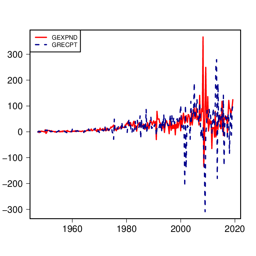

The series are plotted in Figure 3(a). We see that the series start to diverge in the mid 1990s and even more so after year 2000. We estimate the equation and test the null hypothesis of strong sustainability, viz., . FM-OLS estimation of the full sample gives with standard error and -statistic , rejecting the null hypothesis. The result is similar if we include the constant and for bandwidth in place of .
The divergence of the series in mid 1990s in Figure 3(a) may signify a structural break in the relationship. In fact, several studies (e.g. Berenguer-Rico and Carrion-i-Silvestre, 2011) found a break in the 4th quarter of 1996, which could be attributed to the 1997 Clinton tax cut. The study of the properties of the FM-OLS under multicointegration in the presence of structural breaks we leave for future research. But we do estimate the model for the period from 1947:Q1 to 1996:Q4 () finding that with standard error and -statistic , so the cointegrating coefficient is closer to but still statistically different from .
From the Campbell–Shiller work on log-linearization of present value identities we may expect that linear time series models provide better approximations in logarithms of the time series, which has the further advantage of stabilizing variances. The series in logs are plotted in Figure 3(b). We also plot the first differences in levels and in logs in Figure 3. The first differences of logs (Figure 3(d)) show less heteroskedasticity than first differences in levels (Figure 3(c)) so our theory results seem better suited for specification in logs99 9 We thank a referee for this suggestion.. FM-OLS estimation of the full sample in logs gives with standard error and -statistic , rejecting the null hypothesis. The value of the -statistic is similar for the period from 1947:Q1 to 1996:Q4.
We also estimate the cointegration relationship between real revenue and expenditure constructed using the GDP deflator. We take the same data series1010 10 Available at the Journal of Applied Econometrics Data Archive, http://qed.econ.queensu.ca/jae/2011-v26.2/ as in Berenguer-Rico and Carrion-i-Silvestre (2011), but instead of looking at systems (which means working with , and ) we again run FM-OLS on and obtain with standard error and -statistic , rejecting the null hypothesis that revenue and expenditure are cointegrated with coefficient .
6 Conclusion
In a semiparametric triangular representation of cointegrated time series the presence of multicointegration results in a singular long run error variance matrix which has decisive effects on standard methods of estimation and inference in such models. The consequences are higher rates of convergence and non pivotal limit theory in certain directions for estimators such as FM-OLS. Notwithstanding these effects, we show that FM-OLS Wald tests are invariant to singularity under well defined rank conditions and, when those conditions fail, the tests are conservative in certain cases. In particular, simulation experiments show that in such situations the test rejection rates under the null hypothesis are far below nominal levels based on standard asymptotics in singular and near singular cases. We illustrate our methods by analyzing the fiscal sustainability of the US government, testing the hypothesis that government revenue and expenditure are strongly cointegrated with coefficient , where multicointegration naturally arises if bounds are imposed on deviations of debt from revenue.
The results obtained here motivate the development of new robust approaches to estimating cointegrating relationships that allow for the possible presence of multicointegration and that are pivotal in the presence of the singularity it produces. This is an ongoing area of research by the authors.
7 Acknowledgments
This paper has origins in a 2011 Yale Take Home Examination. For various and non-overlapping parts of this research Kheifets acknowledges support from the Russian Science Foundation under project 20-78-10113 (Monte Carlo simulations and the fiscal sustainability evaluation) and the Spanish Ministerio de Ciencia, Innovacion y Universidades under Grant ECO2017-86009-P (econometric theory). Phillips acknowledges support from the National Science Foundation under Grant SES 18-50860 and a Kelly Fellowship at the University of Auckland. This research was supported in part through computational resources of HPC facilities at HSE University.
Appendix A Appendix
A.1 Preliminary Lemmas
We start by stating and proving some results for the rates of convergence and limits of the kernel estimator of the long run variance when . These results are of independent interest and are formulated as separate lemmas. The discussion proceeds and results are stated under the assumptions made in the body of the paper.
The results contribute to general literature on the asymptotic bias and variance of spectral estimates, see e.g. Section V in Hannan (1970). We use ideas from Lemma 8.1 (a), (b), and (g) in Phillips (1995), although that lemma does not directly apply to our case. In particular, the errors that appear in Lemma 8.1 in Phillips (1995) arise from a different source: if the regressor vector is cointegrated, but the cointegrating relationship is unknown, FM-OLS uses the first differences of the full vector in making nonparametric adjustments to OLS, thereby producing linear combination of the first differences of stationary errors which are . In our case it is assumed that is positive definite, i.e. that are full rank nonstationary and are full rank stationary . Instead, multicointegration induces singularity in the augmented regression equation error in (3) so that is with consequential effects on the estimation of the long run covariance matrix .
Consider the case where . Define
where is a kernel function, is a bandwidth parameter, , , and we use in place of to stress that the kernel estimators are calculated with the true errors and .
Lemma 1.
Suppose . Then
- (a)
and
- (b)
- (c)
Next consider the case when the kernel estimators are based on regression residuals , where , and using the true transform define , whereas . Define ,
where we use in place of to stress that the kernel estimators use residuals instead of the true errors .
The following lemmas hold irrespective of the singularity of
Lemma 2.
, , are .
Lemma 3.
If , then for ,
- (a)
- (b)
- (c)
A.2 Proofs of Lemmas 1 - 3
Proof of Lemma 1(a).
By Assumption K, and for , and for some with
We show that , , and .
Mean of . Applying the second order Taylor expansion of function at arguments around ,
and for we can apply the Taylor expansion of function at arguments around , where , giving and then Hence,
and
Mean of By the mean value theorem there exists , such that with mean
whose modulus is dominated by
for .
Variance of .
and from Theorem 9 in Hannan (1970, p. 280). So the variance of the dominant term in is .
Term . Note that . , and . Therefore, .
Term . By Assumption K (b), when . By summability, and . Therefore, and . ∎
Proof of Lemma 1(b).
As above,
and while , for by the same argument as in (a). ∎
Proof of Lemma 1(c).
Similar to (b), for some with
By the same argument as above, and , for , while we show below that the limit of can be simplified and the variance bound of can be improved from in (a) and (b) to in the present case. Thus, the contribution from the variance is of smaller order than for any , with .
Mean of .
and
because and . Note that under stricter conditions on the bandwidth rate this limit could be obtained from Theorem 10 in Hannan (1970, p. 283).
Variance of .
and from Theorem 9 in Hannan (1970, p.280). The variance of the dominant term in is therefore . ∎
Proof of Lemma 2.
Because
because and it follows from the proof of Theorem 3.1 of Phillips (1991b, pp. 432–433) that
If , the last bound can be improved to
similar to the proof of Lemma 8.1(c) of Phillips (1995, pp. 1064–1065). ∎
Proof of Lemma 3.
We apply Lemma 1 to the covariance between and and adjust the limits for the use of residual in place of the true error with an additional term of according to Lemma 2, and obtain parts (b) and (c). Part (a) follows by partial summation formula and applying the above procedure to the term in the brackets:
∎
A.3 Proofs of Propositions
Proof of Proposition 1.
We can write , where the roots of satisfy or . Multicointegration of such a linear process occurs (see Johansen 1992, Engsted and Johansen, 1999) when is a root, so that has reduced rank and is singular. The submatrices and their orthogonal complements are given explicitly below for the present context of the triangular system (1) and (2). In particular, write as
and its derivative
| (7) |
We can write
and , which is an matrix of full rank whenever . Multiplication of by the full rank matrix yields
because
and from (7)
since
It follows that when , we have the rank equivalence , which is the multicointegrating rank in the system defined by (1) and (2). More simply, . ∎
Proof of Proposition 2.
Recall that , so
Also, , so
The numerator matrix of FM-OLS is
Therefore,
| (8) |
From standard weak convergence theory for sample covariances in Phillips and Durlauf (1986) and Phillips (1989)
| (9) | ||||
| (10) | ||||
| (11) |
giving
By construction, has zero long run covariance with the errors that drive the nonstationary component , thereby eliminating the endogeneity from in the long run. Therefore, with any consistent estimators of and , under Assumption K with , and using Lemma 2, we have and , so that by continuous mapping and joint convergence of the components we have
∎
Proof of Proposition 3.
Proof of Proposition 4.
Proof of Proposition 5.
Part (a). The rate of convergence and limit behavior of is established in Lemma 3(c), while the difference is of smaller order and can be neglected, viz.,
By comparing the rates in Part (b) and Part (c) in Lemma 3 we see that the square of the decay rate of exceeds that of , giving the required result.
Part (b). Because of the rates of the FM-OLS estimator established in Proposition 3 and the rate of in Part (a), under the null hypothesis we have for
where is the indicator of . ∎
A.4 Proofs of the Theorems
Proof of Theorem 1.
We have
where
The matrix rotates to , where is and is . Therefore keeps the nonstationary regressors and transforms the original cointegration relationship to a system of two equations with orthogonal long run errors: (i) an equation with errors that has a nonsingular long run variance matrix , and for this equation, , Proposition 2 applies; and (ii) an equation with errors , for which Proposition 3 applies. ∎
Proof of Theorem 2.
Using coordinate rotation, we write the Wald statistic as a sum of several components, corresponding to the nondegenerate and degenerate directions and their cross products. Recall the partitioned matrix inversion formula
where the Shur complement is defined as . We apply the above formula to the variance matrix metric in the Wald test statistic giving
where we take into account that
- (i)
, because isolates the nondegenerate direction;
- (ii)
, which is obtained similar to the proof of Lemma 1(b), and switching from residuals to errors involves differences of order , as in Lemma 2, which are of smaller order for ;
- (iii)
, which can be obtained similar to the proofs of Lemma 1(c) and Proposition 5(a).
Then
using the fact that and from Theorem 1. For , we have , and therefore . ∎
References
- [1] Berenguer-Rico, V. and J.L. Carrion-i-Silvestre (2011) Regime shifts in stock–flow – systems: the case of US fiscal sustainability, Journal of Applied Econometrics 26, 298–321.
- [2] Bohn, H. (2007) Are stationarity and cointegration restrictions really necessary for the intertemporal budget constraint? Journal of Monetary Economics 54, 1837–1847.
- [3] Boswijk, H.P. (2000) Mixed normality and ancillarity in systems. Econometric Theory 16, 878–904.
- [4] Boswijk, H.P. (2010) Mixed normal inference on multicointegration, Econometric Theory 26, 1565–1576.
- [5] D’Erasmo, P.D., Mendoza, E.G. and J. Zhang (2016) What is a Sustainable Public Debt? Handbook of Macroeconomics 2B, 2493–2597.
- [6] Engsted, T., Gonzalo, J. and N. Haldrup (1997) Testing for multicointegration. Economics Letters, 56, 259–266.
- [7] Engsted, T. and S. Johansen (1999) Granger’s representation theorem and multicointegration. In R.F. Engle and H. White (eds.), Cointegration, Causality and Forecasting: Festschrift in Honour of Clive Granger, 200–-212. Oxford University Press.
- [8] Franchi, M. and P. Paruolo (2019) A general inversion theorem for cointegration, Econometric Reviews, 38, 1176–1201.
- [9] Granger, C.W.J. and T.-H. Lee (1990) Multicointegration. In G.F. Rhodes Jr. and T.B. Fomby (eds.), Advances in Econometrics: Cointegration, Spurious Regressions and Unit Roots. 71–-84. JAI Press.
- [10] Hakkio, C. S. and M. Rush (1991) Is the budget deficit too large? Economic Inquiry 29, 429–445.
- [11] Haldrup, N. (1994) The asymptotics of single-equation comtegration regressions with and variables. Journal of Econometrics 63, 151–181.
- [12] Hamilton, J. D. and M. A. Flavin (1986) On the limitations of government borrowing: a framework for empirical testing. American Economic Review 76, 808–816.
- [13] Hannan, E. J. (1970) Multiple Time Series. New York: John Wiley & Sons.
- [14] Haug, A. A. (1991) Cointegration and government borrowing constraints: evidence for the United States. Journal of Business and Economic Statistics 9, 97–101.
- [15] Johansen, S. (1992) A representation of vector autoregressive processes integrated of order 2. Econometric Theory 8, 188–202.
- [16] Johansen, S. (1997) Likelihood analysis of the model. Scandinavian Journal of Statistics 24, 433–462.
- [17] Johansen, S. (2006) Statistical analysis of hypotheses on the cointegrating relations in the model. Journal of Econometrics 132, 81–115.
- [18] Park, J. Y. (1992) Canonical Cointegrating Regressions, Econometrica 60, 119–143.
- [19] Paruolo, P. (2000) Asymptotic efficiency of the two stage estimator in systems. Econometric Theory 16, 524–550.
- [20] Phillips, P. C. B. (1989) Partially Identified Econometric Models, Econometric Theory 5, 181–240.
- [21] Phillips, P. C. B. (1991) Optimal Inference in Cointegrated Systems, Econometrica 59, 283-306.
- [22] Phillips, P. C. B. (1991b) Spectral Regression for Cointegrated Time Series, in Nonparametric and Semiparametric Methods in Economics and Statistics, ed. by W. Barnett, J. Powell, and G. Tauchen. New York: Cambridge University Press.
- [23] Phillips, P. C. B. (1995) Fully Modified Least Squares and Vector Autoregression, Econometrica 63, 1023–1078.
- [24] Phillips, P.C.B. (2014) Optimal estimation of cointegrated systems with irrelevant instruments. Journal of Econometrics 178, 210–224.
- [25] Phillips, P. C. B. (2016) Inference in near-singular regression. Advances in Econometrics 36, 461–486.
- [26] Phillips, P. C. B. and S.N. Durlauf (1986) Multiple Time Series Regression with Integrated Processes, Review of Economic Studies 53, 473–495.
- [27] Phillips, P. C. B. and B. E. Hansen (1990) Statistical Inference in Instrumental Variables Regression with Processes, Review of Economic Studies 57, 99–125.
- [28] Phillips, P. C. B. and I. L. Kheifets (2019) On Multicointegration. Working Paper, Yale University. Presented at the Rimini Time Series Conference, Larnica, Cyprus, June 2019.
- [29] Phillips, P. C. B. and M. Loretan (1991) Estimating Long-Run Economic Equilibria. The Review of Economic Studies 58, 407–436.
- [30] Phillips, P. C. B. and V. Solo (1992) Asymptotics for Linear Processes. Annals of Statistics 20, 971–1001.
- [31] Priestley, M.B. (1981) Spectral Analysis and Time Series. Academic Press Inc, New York.
- [32] Quintos, C.E. (1995) Sustainability of the deficit process with structural shifts. Journal of Business and Economic Statistics 13, 409–417.
- [33] Toda, H. Y. and P.C.B. Phillips (1993) Vector Autoregressions and Causality Econometrica 61, 1367–1393.
- [34] Trehan, B., and C. Walsh (1991) Testing intertemporal budget constraints: theory and applications to U.S. Federal budget and current account deficits. Journal of Money, Credit and Banking 23, 210–223.