Dynamic electron-phonon and spin-phonon interactions due to inertia

In the adiabatic Born-Oppenheimer approximation, the electronic degrees of freedom are separated from the ionic degrees of freedom. Excitations of the ionic degrees of freedom, such as phonons in crystals and vibrations, torsions, and rotations in molecules can be resonantly driven by state-of-the-art experiments with coherent high intensity THz laser beams Salén et al. 2019; Kampfrath et al. 2013. This opens the prospect of coherent control of emergence in quantum materials and the design of new phases of matter Först et al. 2011; Subedi et al. 2014; Mankowsky et al. 2016. For example, the coherent control of local dipoles induce a transient magnetization in the framework of the dynamical multiferroicity Rebane 1983; Juraschek et al. 2017. The strength of this effect is predicted to be in the order of the nuclear magneton Juraschek et al. 2017; Juraschek et al. 2019; Geilhufe et al. 2021a. However, recent experiments measuring the magneto-optical Kerr effect hint towards much higher magnetic moments Basini et al.. In the phonon Zeeman effect, left- and right-handed circularly polarized phonon modes split in a magnetic field. Again, the measured phonon Zeeman splitting seems to be much larger than theoretical estimates Cheng et al. 2020; Schaack 1977; Schaack 1976; Juraschek et al. 2020; Baydin et al. 2021; Juraschek and Spaldin 2019. This discrepancy has initiated a debate on phonon angular momenta Zhang and Niu 2014; Garanin and Chudnovsky 2015; Rückriegel et al. 2020, non-linear or anharmonic corrections Baydin et al. 2021, topological features of effective charges Ren et al. 2021, and angular momentum transfer from ionic to electronic degrees of freedom Geilhufe et al. 2021a.

Electron-phonon interactions are commonly described using the Fröhlich Hamiltonian Fröhlich 1937, which can be extended towards including spin-phonon terms Mattuck and Strandberg 1960. In the present paper we aim to provide a different microscopic model coupling ionic motion to electronic degrees of freedom. This model is based on inertial effects experienced by electrons bound to a moving ion. Considering the circular motion of an ion due to a phonon excitation (see Fig. 1), a local inertial frame accelerates relative to a selected ion. However, a local observer on the ion finds themselves in a noninertial frame. As a result, inertial effects emerge. In classical mechanics, a rotating coordinate system induces fictious forces like the Coriolis force $\boldsymbol{F}_{\text{Coriolois}}=2\boldsymbol{p}\times\boldsymbol{\omega}$ or the centrifugal force $F_{\text{Cent.}}=m\omega^{2}\boldsymbol{d}$, where $\boldsymbol{\omega}$ ($\omega$) is the angular velocity (frequency), $\boldsymbol{d}$ the radius determined by the ionic displacement from the equilibrium position, $\boldsymbol{p}$ the momentum of a probe particle and $m$ the corresponding mass. Promoting the fictious forces to an energy by multipling with the position of the probe particle, reveals the coupling of the angular velocity with the probe particle angular momentum $E=\boldsymbol{F}_{\text{Coriolois}}\cdot\boldsymbol{r}=2\boldsymbol{\omega}\cdot\boldsymbol{L}$ or a centrifugal-force coupling comparable to the coupling of an applied electric field, $E=\boldsymbol{F}_{\text{Cent.}}\cdot\boldsymbol{r}=m\omega^{2}\boldsymbol{d}\cdot\boldsymbol{r}$. Subsequenty, we review that the Coriolis and Centrifugal effects also emerge in quantum systems and provide realistic estimates for resulting electron-phonon and spin-phonon interactions.

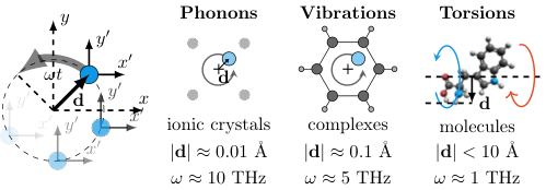
Inertial effects of quantum systems have attracted great attention in astronomical settings or collision experiments. Related to the classical Coriolis force, the rotation of a quantum system leads to the well-known spin-rotation coupling $\sim\boldsymbol{\omega}\cdot\boldsymbol{J}$, with $\boldsymbol{J}=\boldsymbol{L}+\boldsymbol{S}$ the total angular momentum. Variants of this coupling were derived by Werner et al. Werner et al. 1979, Mashoon Mashhoon 1988, Müller and Greiner Müller and Greiner 1976, Hehl and Ni Hehl and Ni 1990, and Ryder Ryder 2008. Spin-rotation coupling has been observed using neutron interferometry Mashhoon 1988; Danner et al. 2020, where two perpendicular neutron beams accumulate a phase shift due to the earth rotation. Note that the rotation frequency of the earth $\approx~70\mu\text{Hz}$ is about 17 orders of magnitude smaller than the ionic motion in a crystalline lattice. Quantum effects for accelerating references frames were discussed, e.g., by Hehl and Ni Hehl and Ni 1990, Hehl Hehl 1985, and Ryder Ryder 2008. With the prospect of mechanically inducing a topological phase and spin-currents, the idea of tuning quantum states by accelerations has been developed, e.g., for samples coupled to microwave resonators, inducing tiny circular motions Basu and Chowdhury 2013; Matsuo et al. 2011. Inertial effects of spins were recently discussed in the context of spin dynamics and the Landau–Lifshitz–Gilbert equation, describing e.g. spin nutations Neeraj et al. 2021; Bhattacharjee et al. 2012; Böttcher et al. 2011; Ciornei et al. 2011.

To discuss the coupling of the ionic motion to the electron, we focus on a single ion moving on a circular orbit around the Cartesian $z$-axis, with frequency $\omega$ and displacement $\boldsymbol{d}=d(\cos(\omega t),\sin(\omega t),0)$. Examples are summarized in Fig. 1. To obtain access to the spin degrees of freedom, we follow the formalism of Hehl and Ni Hehl and Ni 1990 and formulate the corresponding Dirac equation in an accelerating frame and take the non-reativistic limit to the Schrödinger equation.

By definition of the coordinate system, we obtain for the four-velocity and the four-acceleration

with the Lorentz factor $\gamma=\left(1-\frac{\boldsymbol{d}^{2}\omega^{2}}{c^{2}}\right)^{-\frac{1}{2}}\approx 1$. The coordinate tetrad $e_{a}$ carried along with the observer, is a rest frame for the observer. Hence, the observer’s time axis coincides with the four-velocity $e_{0}^{~\mu}=u^{\mu}$. At the same time, the tetrad $e_{\mu}$ must remain orthonormal. We apply generalized Fermi-Walker transport, to describe the accelerating and rotating observer and the tetrad transported along the observer’s world line, parametrized by the proper time $\tau$,

Here, the generalzed Fermi-Walker transport tensor $\Omega_{\text{FW}}$ splits into a non-rotating and a rotating part Hehl et al. 1991; Misner et al. 1973

Here, $\epsilon^{\alpha\beta\mu\nu}$ is the antisymmetric Levi-Civita tensor. The infinitesimal line element is

In the observer’s local frame, the Dirac equation is written as

Here, $\Psi$ is a four-spinor, $m$ the electron mass, and $\gamma^{a}$ the Dirac $\gamma$-matrices, $\left\{\gamma^{\mu},\gamma^{\nu}\right\}=\eta^{\mu\nu}$. $D_{a}=\partial_{a}-\frac{\mathrm{i}}{4}\sigma^{bc}\Gamma_{bca}$ is the covariant derivative, with $\sigma^{ab}=\frac{\mathrm{i}}{2}\left[\gamma^{a},\gamma^{b}\right]$ and $\Gamma_{bca}$ the connection coefficient Hehl 1985; Hehl and Ni 1990.

Following Refs. Hehl and Ni 1990; Hehl et al. 1991 and evaluating equation (5) for our example gives the following Dirac equation including inertial terms,

Note, that we now use the Dirac matrices $\alpha_{i}$ and $\beta$, with $\left\{\alpha_{i},\alpha_{j}\right\}=\left\{\alpha_{i},\beta\right\}=0$ and $\alpha_{i}^{2}=\beta^{2}=1$. They are related to the $\gamma$ matrices by $\gamma^{0}=\beta$ and $\gamma^{i}=\beta\alpha_{i}$. The conventional Dirac Hamiltonian $H=c\boldsymbol{\alpha}\cdot\boldsymbol{p}+\beta mc^{2}$ is extended by three dynamic terms. The first two dynamic terms correspond to the centrifugal force $\boldsymbol{F}_{\text{Cent.}}=m\omega^{2}\boldsymbol{d}$, a correction to the kinetic energy $\frac{\gamma^{2}}{2mc}\left\{\boldsymbol{F}_{\text{Cent.}}\cdot\boldsymbol{r},\boldsymbol{p}\cdot\boldsymbol{\alpha}\right\}$ and a correction to the mass, $\gamma^{2}\left(\boldsymbol{F}_{\text{Cent.}}\cdot\boldsymbol{r}\right)$. The third term is the spin-rotation coupling, corresponding to the Coriolis force. $\boldsymbol{J}$ is the total angular momentum operator, $\boldsymbol{J}=\boldsymbol{L}+\boldsymbol{S}$.

As we are mainly concerned with molecules and solids, we continue by evaluating the non-relativistic limit of the Dirac equation (6). We perform the Foldy-Wouthuysen transformation as described by Bjorken and Drell Bjorken and Drell 1964. We rearrange the Dirac Hamiltonian as $H=\beta mc^{2}+\mathcal{O}+\mathcal{E}$, with the odd terms $\mathcal{O}=c\boldsymbol{\alpha}\cdot\boldsymbol{p}-\frac{\gamma^{2}}{2mc}\left\{\boldsymbol{F}_{\text{Cent.}}\cdot\boldsymbol{r},\boldsymbol{p}\cdot\boldsymbol{\alpha}\right\}$ and the even terms $\mathcal{E}=-\beta\gamma^{2}\left(\boldsymbol{F}_{\text{Cent.}}\cdot\boldsymbol{r}\right)-\boldsymbol{\omega}\cdot\boldsymbol{J}$. The transformed Hamiltonian up to the order of $\frac{1}{mc^{2}}$ is given by $H\approx\beta\left[mc^{2}+\frac{\mathcal{O}^{2}}{2mc^{2}}+\mathcal{E}+\dots\right]$. Evaluating $\mathcal{O}^{2}$ up to $\frac{1}{mc^{2}}$ and removing the rest mass term in the particle channel gives the following Schrödinger equation, including four dynamic correction terms

In comparison to equation (6), equation (7) determines a two-spinor $\Phi$ (due to the spin degrees of freedom, (7) could also be called Pauli equation).

For brevity, we ommitted writing down the coupling to an electromagnetic field in this discussion. In general, we assume electrons being localized on an atom, which requires a confining potential $V(\boldsymbol{r}+\boldsymbol{d}(t))$, or, $V(\boldsymbol{r})$ in the local coordinate frame. In the non-relativistic limit, a scalar potential in the Dirac equation leads to a scalar potential plus spin-orbit interaction and the Darwin term Bjorken and Drell 1964; Strange et al. 1989. However, to lowest order, no additional corrections due to the moving frame emerge (compare also Ref. Müller and Greiner 1976). Hence, writing down (7) implicitly encourages the reader to add respective potential terms.

We continue discussing the individual terms. The most prominent term is the spin-rotation coupling, or Mashoon-Zeeman term. In fact, comparing the Zeeman coupling $\mu_{B}g_{J}\boldsymbol{B}\cdot\boldsymbol{J}$ to the spin-rotation coupling, allows us to identify a 1 THz rotation with a 10 T magnetic field (note that the inertial spin-rotation coupling is different from the spin-rotation coupling $\sim\boldsymbol{J}\cdot\mathrm{M}\cdot\boldsymbol{I}$, coupling the electronic spin $\boldsymbol{J}$ to the nuclear spin $\boldsymbol{I}$, via the tensor $\mathrm{M}$). Although this seems like a significant effect, it has only sparsely been discussed in the context of rotating molecules Shen and He 2003.

Furthermore, there are three terms connected to the centrifugal force. For the electron mass of $9.1\times 10^{-31}~\text{kg}$, the typical atomic distances of $1~\text{\AA}$, and vibrational frequencies of THz, the centrifugal force is $\approx 10^{-16}~\text{N}$. Comparing this value to a fictuous electric field applied to an electron, this corresponds to a field strength of $\approx 10~\text{Vcm}^{-1}$. In general, the action of the centrifugal force is time-dependent due to the circular motion of the ions. However, the ionic motion is in the THz regime, corresponding to the meV energy range. Hence, for sufficiently large level splitting, we apply the adiabatic approximation, assuming that the ionic motion is much slower than the electronic degrees of freedom. As a consequence, the electronic system remains in the ground state.

The first term arising due to the centrifugal force is the centrifugal field coupling $\gamma^{2}\boldsymbol{F}_{\text{Cent.}}\cdot\boldsymbol{r}$. The term occurs both in the relativistic theory (6) and the nonrelativistic limit (7). The centrifugal field coupling is linear in the position vector $\boldsymbol{r}$ and inversion odd. Similar to the stark effect, it only introduces a correction in linear perturbation theory if inversion symmetry is broken, or if a set of degenerate levels contains parity even and odd energy levels, e.g., as for the excited hydrogen levels in the approximation of the Schrödinger equation Schwabl 2007. The centrifugal field coupling requires matrix elements between states with angular momentum $l$ and $l\pm 1$, i.e., $-e\left(\Psi_{nlm}|\boldsymbol{E}_{p}\cdot\boldsymbol{r}|\Psi_{n^{\prime}l^{\prime}m^{\prime}}\right)=\delta_{nn^{\prime}}\delta_{l,l^{\prime}\pm 1}\delta_{mm^{\prime}}\left(\Psi_{nlm}|\boldsymbol{E}_{p}\cdot\boldsymbol{r}|\Psi_{n^{\prime}l^{\prime}m^{\prime}}\right)$. For example, for the hydrogen $n=2$ states with $l=0$ and $l^{\prime}=1$, the resulting energy correction is $\Delta E=\pm 3\gamma^{2}\left|\boldsymbol{F}_{\text{Cent.}}\right|a_{0}$, with $a_{0}$ the Bohr radius. The corresponding correction for a typical phonon is tiny, $\sim\mu\text{eV}$. The same order of magnitude holds in case of the relativistic electronic levels of the hydrogen atoms, as discussed e.g. by Blackman and Series Blackman and Series 1973 on the example of the conventional Stark effect. Still, the level splitting due to centrifugal field is much larger than e.g. the observable Lamb shift between the $s_{1/2}$ and $p_{1/2}$ states of $\approx 1057~\text{MHz}$ I. Eides et al. 2001. Following Marxer Marxer 1995, we note that the Stark effect and the inertial field coupling roughly go as $\sim n/Z$, with $Z$ the atomic number.

The second term is the centrifugal spin orbit coupling or Rashba-Hehl-Ni spin-orbit coupling $\sim\frac{\gamma^{2}}{2m^{2}c^{2}}\,\boldsymbol{F}_{\text{Cent.}}\cdot(\boldsymbol{S}\times\boldsymbol{p})=\frac{\alpha_{p}}{\hbar}\,\hat{\boldsymbol{z}}\cdot\left(\boldsymbol{\sigma}\times\boldsymbol{p}\right)$. Note that we choose the Cartesian $z$-axis to point along the ionic displacement $\boldsymbol{d}$, i.e., in direction of the centrifugal force. The second form underlines the connection to the Rashba spin-orbit interaction. The corresponding Rashba-Hehl-Ni coefficient is given by

Given the electron rest mass of $\approx 0.51~\text{MeV}$ and THz frequencies $\hbar\omega\approx 4.1~\text{meV}$, the Rashba-Hehl-Ni coefficient would take values of $\alpha_{p}\approx 10^{-12}~\text{eV\AA}$. Similar to the Rashba effect, The Rashba-Hehl-Ni spin-orbit coupling is a consequence of the symmetry breaking associated to the centrifugal force. For example, starting from a spherically symmetric potential, the centrifugal force induces a symmetry breaking to a uniaxial symmetry. As a result, the Rashba-Hehl-Ni spin-orbit coupling is allowed.

The similar order of magnitude holds for the third centrifugal correction, the centrifugal redshift $\sim\frac{\gamma^{2}}{2m^{2}c^{2}}\boldsymbol{p}\cdot\left(\boldsymbol{F}_{\text{Cent.}}\cdot\boldsymbol{r}\right)\cdot\boldsymbol{p}$. It has the same pre-factor as the centrifugal spin-orbit coupling, being a $\frac{1}{mc^{2}}$-correction. Similarly, as the centrifugal field coupling, the centrifugal redshift is inversion-odd, introducing a weak overlap of inversion even and odd states. In the case of periodic solids the term manifests as a correction to the dispersion relation.

We continue by modelling the pseudo electric field using a realistic, but generic 2D model. We excite a vibrational displacement $\boldsymbol{u}$ by an intense circularly polarized laser pulse $\boldsymbol{E}(t)$, acting in the $xy$-plane. The displacement follows the damped classical equation of motion

For simplicity, we couple the electric field to a localized charge, which is a good approximation for many ionic crystals. In a more realistic setup, one would couple the field to the Born effective charge, describing the response of the macroscopic polarization per unit cell to the displacement of an atom Ghosez et al. 1998. The dynamical matrix $\mathrm{K}$ has two degenerate vibrational modes (along the Cartesian $x$ and $y$ directions) with eigenfrequency of $f=10~\text{THz}$. We choose a resonant strong circularly polarized Gaussian laser pulse, with a peak field of 500 kVcm^-1 and a pulse width of 2 ps. The damping parameter is chosen to be $\eta=0.15\times 2\pi~\text{THz}$. We use a charge of $q=1$ and a mass of $m=10~\text{u}$.

The outcome of the simulation is shown in Fig. 2. For better comparison of the strength of the centrifugal force, we introduce the pseudoelectric field $\boldsymbol{E}_{p}$,

Depending on the damping, the peak of the atomic displacement ($\approx 0.03~\text{\AA}$) and the centrifugal force or pseudo electric field ($\approx 18~\text{Vcm}^{-1}$) emerge about 1 ps after the peak of the initial laser field. Both, the displacement and the centrifugal force decay slowly and persist for about one order of magnitude longer than the lifetime of the initial laser pulse. Hence, experimentally observable consequences of inertial effects should be probed shortly after the laser pulse fully decayed.

We close the paper with a summary and outlook. We showed that the circular motion of ions in molecules and crystals induces local inertial effects on electrons. We introduced the spin rotation coupling corresponding to a Coriolis force and three corrections corresponding to the centrifugal force: the centrifugal field coupling; the centrifugal Rashba-Hehl-Ni spin-orbit coupling; the centrifugal redshift. The strength of the spin-rotation coupling is significant and introduces a Zeeman-like splitting in the meV range. The strength of the centrifugal terms scale as $\sim\omega^{2}\boldsymbol{d}$. Hence, they grow linearly in the displacement or rotation radius $\boldsymbol{d}$ and quadratically in the rotation frequency $\omega$. Such ionic motion can be induced by circularly polarized laser pulses. We could show that the lifetime of the inertial pseudo electric field is much longer than the lifetime of the initial laser pulse, depending on the material specific damping.

The inertial effects open new perspectives on quantum and spin control in matter. As strongly localized effects, they allow for the precise manipulation of energy levels and spin around specified ions by vibrational degrees of freedom. Vibrations and phonons can be simulated with high accuracy using state-of-the-art computational tools Baroni et al. 2001; Togo and Tanaka 2015; Wang et al. 2016. They allow to guide experiments using THz radiation towards a selective control of the desired quantum state. Even though, the pseudo electric field is localized on a moving ion, it will also control the overlap of electronic states in molecular or periodic systems. As a consequence, the three terms will arise in quantum many-body systems, potentially affecting quasi-electron excitations in matter. Here, the effective mass of the quasi-electron could be much lower than the actual electron mass, as is the case in many semiconductors. For example, in silicon the light-hole mass is about a tenth of the actual electron mass Ramos et al. 2001. Such a lowered quasi-electron mass would boost the inertial Rashba parameter $\alpha_{p}\sim m^{-1}$. In general, the challenge is to extend both, $\omega$ and $\boldsymbol{d}$. Torsions in large molecules might provide the promising platform for inertial effects.

Selecting relevant target materials is outside the scope of this paper. We note that recent progress in materials informatics might allow identifying experimentally feasible materials Ramprasad et al. 2017; Geilhufe et al. 2021b; Horton et al. 2021; Greenaway and Jelfs 2021. The target space was defined throughout the present work. In particular, soft organic crystals, molecules, and metal organic frameworks are a promising materials class. Following implementations of static electric fields in ab initio codes, we also see the prospect of implementing the inertial correction terms into ab initio codes, e.g., in the framework of the density functional perturbation theory Refson et al. 2006; Wu et al. 2005. While the majority of the discussion concerned the non-relativistic limit, a separate discussion for the relativistic effects in matter and their implementation into ab initio codes would be necessary Geilhufe et al. 2015; Wills and Mattsson 2012; Huhne et al. 1998; Strange et al. 1989.

Acknowledgment. We are grateful to A. V. Balatsky, S. Bonetti, M. Basini, A. Brandenburg, J. D. Rinehart, V. Juričić, W. Hergert, O. Tjernberg, and M. Månson for inspiring discussions. We acknowledge support from research funding granted to A. V. Balatsky, i.e., VILLUM FONDEN via the Centre of Excellence for Dirac Materials (Grant No. 11744), the European Research Council under the European Union Seventh Framework ERS-2018-SYG 810451 HERO, the Knut and Alice Wallenberg Foundation KAW 2018.0104. Computational resources were provided by the Swedish National Infrastructure for Computing (SNIC) via the High Performance Computing Centre North (HPC2N) and the Uppsala Multidisciplinary Centre for Advanced Computational Science (UPPMAX).

References

- Salén et al. (2019) P. Salén, M. Basini, S. Bonetti, J. Hebling, M. Krasilnikov, A. Y. Nikitin, G. Shamuilov, Z. Tibai, V. Zhaunerchyk, and V. Goryashko, Physics Reports 836, 1 (2019).
- Kampfrath et al. (2013) T. Kampfrath, K. Tanaka, and K. A. Nelson, Nature Photonics 7, 680 (2013).
- Först et al. (2011) M. Först, C. Manzoni, S. Kaiser, Y. Tomioka, Y.-n. Tokura, R. Merlin, and A. Cavalleri, Nature Physics 7, 854 (2011).
- Subedi et al. (2014) A. Subedi, A. Cavalleri, and A. Georges, Phys. Rev. B 89, 220301(R) (2014).
- Mankowsky et al. (2016) R. Mankowsky, M. Först, and A. Cavalleri, 79, 064503 (2016).
- Rebane (1983) Y. T. Rebane, Soviet Journal of Experimental and Theoretical Physics 57, 1356 (1983).
- Juraschek et al. (2017) D. M. Juraschek, M. Fechner, A. V. Balatsky, and N. A. Spaldin, Physical Review Materials 1, 014401 (2017).
- Juraschek et al. (2019) D. M. Juraschek, Q. N. Meier, M. Trassin, S. E. Trolier-McKinstry, C. L. Degen, and N. A. Spaldin, Phys. Rev. Lett. 123, 127601 (2019).
- Geilhufe et al. (2021a) R. M. Geilhufe, V. Juričić, S. Bonetti, J.-X. Zhu, and A. V. Balatsky, Physical Review Research 3, L022011 (2021a).
- (10) M. Basini, M. Pancaldi, B. Wehinger, T. Terumasa, M. C. Hoffmann, A. V. Balatsky, and S. Bonetti, in progress .
- Cheng et al. (2020) B. Cheng, T. Schumann, Y. Wang, X. Zhang, D. Barbalas, S. Stemmer, and N. P. Armitage, Nano Letters 20, 5991 (2020).
- Schaack (1977) G. Schaack, Zeitschrift für Physik B Condensed Matter 26, 49 (1977).
- Schaack (1976) G. Schaack, Journal of Physics C: Solid State Physics 9, L297 (1976).
- Juraschek et al. (2020) D. M. Juraschek, T. Neuman, and P. Narang, arXiv preprint arXiv:2007.10556 (2020).
- Baydin et al. (2021) A. Baydin, F. G. Hernandez, M. Rodriguez-Vega, A. K. Okazaki, F. Tay, G. T. Noe II, I. Katayama, J. Takeda, H. Nojiri, P. H. Rappl, et al., arXiv preprint arXiv:2107.07616 (2021).
- Juraschek and Spaldin (2019) D. M. Juraschek and N. A. Spaldin, Physical Review Materials 3, 064405 (2019).
- Zhang and Niu (2014) L. Zhang and Q. Niu, Phys. Rev. Lett. 112, 085503 (2014).
- Garanin and Chudnovsky (2015) D. A. Garanin and E. M. Chudnovsky, Phys. Rev. B 92, 024421 (2015).
- Rückriegel et al. (2020) A. Rückriegel, S. Streib, G. E. W. Bauer, and R. A. Duine, Phys. Rev. B 101, 104402 (2020).
- Ren et al. (2021) Y. Ren, C. Xiao, D. Saparov, and Q. Niu, arXiv preprint arXiv:2103.05786 (2021).
- Fröhlich (1937) H. Fröhlich, Proceedings of the Royal Society of London. Series A-Mathematical and Physical Sciences 160, 230 (1937).
- Mattuck and Strandberg (1960) R. D. Mattuck and M. Strandberg, Physical Review 119, 1204 (1960).
- Shimanouchi et al. (1973) T. Shimanouchi et al., Tables of molecular vibrational frequencies (US Government Printing Office, 1973).
- Bell (2005) S. Bell, Spectrochimica Acta Part A: Molecular and Biomolecular Spectroscopy 61, 1471 (2005).
- Yu et al. (2004) B. Yu, F. Zeng, Y. Yang, Q. Xing, A. Chechin, X. Xin, I. Zeylikovich, and R. Alfano, Biophysical Journal 86, 1649 (2004).
- Werner et al. (1979) S. A. Werner, J.-L. Staudenmann, and R. Colella, Physical Review Letters 42, 1103 (1979).
- Mashhoon (1988) B. Mashhoon, Physical Review Letters 61, 2639 (1988).
- Müller and Greiner (1976) B. Müller and W. Greiner, Zeitschrift für Naturforschung A 31, 1 (1976).
- Hehl and Ni (1990) F. W. Hehl and W.-T. Ni, Physical Review D 42, 2045 (1990).
- Ryder (2008) L. Ryder, General Relativity and Gravitation 40, 1111 (2008).
- Danner et al. (2020) A. Danner, B. Demirel, W. Kersten, H. Lemmel, R. Wagner, S. Sponar, and Y. Hasegawa, npj Quantum Information 6, 1 (2020).
- Hehl (1985) F. W. Hehl, Foundations of Physics 15, 451 (1985).
- Basu and Chowdhury (2013) B. Basu and D. Chowdhury, Annals of Physics 335, 47 (2013).
- Matsuo et al. (2011) M. Matsuo, J. Ieda, E. Saitoh, and S. Maekawa, Physical Review B 84, 104410 (2011).
- Neeraj et al. (2021) K. Neeraj, N. Awari, S. Kovalev, D. Polley, N. Z. Hagström, S. S. P. K. Arekapudi, A. Semisalova, K. Lenz, B. Green, J.-C. Deinert, et al., Nature Physics 17, 245 (2021).
- Bhattacharjee et al. (2012) S. Bhattacharjee, L. Nordström, and J. Fransson, Physical review letters 108, 057204 (2012).
- Böttcher et al. (2011) D. Böttcher, A. Ernst, and J. Henk, Journal of Physics: Condensed Matter 23, 296003 (2011).
- Ciornei et al. (2011) M.-C. Ciornei, J. Rubí, and J.-E. Wegrowe, Physical Review B 83, 020410(R) (2011).
- Hehl et al. (1991) F. W. Hehl, J. Lemke, and E. W. Mielke, “Two lectures on fermions and gravity,” in Geometry and Theoretical Physics, edited by J. Debrus and A. C. Hirshfeld (Springer Berlin Heidelberg, Berlin, Heidelberg, 1991) pp. 56–140.
- Misner et al. (1973) C. W. Misner, K. S. Thorne, and J. A. Wheeler, Gravitation (Macmillan, 1973).
- Bjorken and Drell (1964) J. D. Bjorken and S. D. Drell, Relativistic quantum mechanics (McGraw-Hill, 1964).
- Strange et al. (1989) P. Strange, H. Ebert, J. Staunton, and B. L. Gyorffy, Journal of Physics: Condensed Matter 1, 2959 (1989).
- Shen and He (2003) J.-Q. Shen and S.-L. He, Physical Review B 68, 195421 (2003).
- Schwabl (2007) F. Schwabl, Quantum Mechanics (Springer Berlin Heidelberg, 2007).
- Blackman and Series (1973) J. Blackman and G. Series, Journal of Physics B: Atomic and Molecular Physics 6, 1090 (1973).
- I. Eides et al. (2001) M. I. Eides, H. Grotch, and V. A. Shelyuto, Physics Reports 342, 63 (2001).
- Marxer (1995) H. Marxer, Journal of Physics B: Atomic, Molecular and Optical Physics 28, 341 (1995).
- Ghosez et al. (1998) P. Ghosez, J.-P. Michenaud, and X. Gonze, Physical Review B 58, 6224 (1998).
- Baroni et al. (2001) S. Baroni, S. de Gironcoli, A. Dal Corso, and P. Giannozzi, Reviews of Modern Physics 73, 515 (2001).
- Togo and Tanaka (2015) A. Togo and I. Tanaka, Scripta Materialia 108, 1 (2015).
- Wang et al. (2016) Y. Wang, S.-L. Shang, H. Fang, Z.-K. Liu, and L.-Q. Chen, npj Computational Materials 2, 1 (2016).
- Ramos et al. (2001) L. E. Ramos, L. K. Teles, L. M. R. Scolfaro, J. L. P. Castineira, A. L. Rosa, and J. R. Leite, Physical Review B 63, 165210 (2001).
- Ramprasad et al. (2017) R. Ramprasad, R. Batra, G. Pilania, A. Mannodi-Kanakkithodi, and C. Kim, npj Computational Materials 3, 1 (2017).
- Geilhufe et al. (2021b) R. M. Geilhufe, B. Olsthoorn, and A. V. Balatsky, Nature Physics 17, 152 (2021b).
- Horton et al. (2021) M. Horton, S. Dwaraknath, and K. Persson, Nature Computational Science 1, 3 (2021).
- Greenaway and Jelfs (2021) R. L. Greenaway and K. E. Jelfs, Advanced Materials 33, 2004831 (2021), https://onlinelibrary.wiley.com/doi/pdf/10.1002/adma.202004831 .
- Refson et al. (2006) K. Refson, P. R. Tulip, and S. J. Clark, Physical Review B 73, 155114 (2006).
- Wu et al. (2005) X. Wu, D. Vanderbilt, and D. R. Hamann, Physical Review B 72, 035105 (2005).
- Geilhufe et al. (2015) M. Geilhufe, S. Achilles, M. A. Köbis, M. Arnold, I. Mertig, W. Hergert, and A. Ernst, Journal of Physics: Condensed Matter 27, 435202 (2015).
- Wills and Mattsson (2012) J. M. Wills and A. E. Mattsson, The Dirac equation in electronic structure calculations: Accurate evaluation of DFT predictions for actinides, Tech. Rep. (Los Alamos National Lab.(LANL), Los Alamos, NM (United States), 2012).
- Huhne et al. (1998) T. Huhne, C. Zecha, H. Ebert, P. H. Dederichs, and R. Zeller, Physical Review B 58, 10236 (1998).