Primordial black holes and stochastic gravitational wave background from inflation with a noncanonical spectator field

Rong-Gen Cai Email: cairg@itp.ac.cn Affiliation: CAS Key Laboratory of Theoretical Physics, Institute of Theoretical Physics, Chinese Academy of Sciences, Beijing 100190, China Affiliation: School of Physical Sciences, University of Chinese Academy of Sciences, Beijing 100049, China Chao Chen Email: cchao012@mail.ustc.edu.cn Affiliation: Department of Astronomy, School of Physical Sciences, University of Science and Technology of China, Hefei, Anhui 230026, China Affiliation: Jockey Club Institute for Advanced Study, The Hong Kong University of Science and Technology, Hong Kong SAR, China Chengjie Fu Corresponding author: fucj@itp.ac.cn Affiliation: CAS Key Laboratory of Theoretical Physics, Institute of Theoretical Physics, Chinese Academy of Sciences, Beijing 100190, China

Abstract

We investigate the enhancement of the curvature perturbations in a single-field slow-roll inflation with a spectator scalar field kinetically coupled to the inflaton. The coupling term with a periodic function of inflaton triggers the exponential growth of the spectator field perturbations, which indirectly amplifies the curvature perturbations to produce a sizable abundance of primordial black holes (PBHs). This scenario is found to be insensitive to the inflationary background. We study two distinct populations of the stochastic gravitational wave background (SGWB) produced in this scenario, i.e., induced by the scalar perturbations during the inflationary era and the radiation-dominated era, respectively. With the appropriate choices of parameter space, we consider two PBH mass windows of great interest. One is PBHs of masses $\mathcal{O}(10^{-12})M_{\odot}$ that can be a vital component of dark matter, and the predicted total energy spectrum of SGWB shows a unique profile and is detectable by LISA and Taiji. The other is PBHs of masses $\mathcal{O}(10)M_{\odot}$ which can provide consistent explanation for the LIGO-Virgo events. More interestingly, the predicted gravitational wave signal from the radiation-dominated era may account for the NANOGrav 12.5-yr results.

I Introduction

A region could collapse to a black hole by self-gravitation in the very early Universe as a result of initial overlarge density fluctuations Hawking 1971; Carr and Hawking 1974; Carr 1975. These primordial black holes (PBHs), in general, span a wide mass range from tens of micrograms to millions of solar masses due to their formation mechanism which is different from that of BHs who have stellar origins. In view of this promising feature, PBHs within different mass windows were expected to relate to a variety of cosmological and astronomical phenomena Belotsky et al. 2014; Carr et al. 2016; Carr and Kuhnel 2020; Bird et al. 2016; Sasaki et al. 2016. One of the major motivations to study PBHs is that they could serve as a reasonable candidate for the whole or an appreciable portion of dark matter (DM) which comprises $25\%$ of the critical density of our Universe Belotsky et al. 2014; Carr et al. 2016; Carr and Kuhnel 2020. In particular, the suggestion that the gravitational waves (GWs) were generated by the coalescence of PBH binaries has attracted much attention in recent years with the LIGO-Virgo detection Abbott et al. 2016a; Abbott et al. 2016b; Abbott et al. 2017; Mukherjee and Silk 2021; Mukherjee et al. 2021. Shortly after the first detection of the GW event, GW150914 Abbott et al. 2016a, Bird et al. Bird et al. 2016 found that the merger rate of PBHs with masses of $\sim 30M_{\odot}$ falls within the range of $2$ – $53$ Gpc^-3 yr^-1 inferred from GW150914, and Sasaki et al. Sasaki et al. 2016 argued that the expected PBH merger rate can be made compatible if PBHs constitute $\mathcal{O}(1)$ ‰ of DM.

The induced GWs associated with PBH formation have attracted great attention in recent years. According to second-order cosmological perturbation theory Matarrese et al. 1998; Noh and Hwang 2004; Ananda et al. 2007; Baumann et al. 2007; Wang and Zhang 2017; Domènech and Sasaki 2018, the scalar perturbations would provide anisotropic stress via the nonlinear couplings and result in the generation of GWs. Hence, the overlarge primordial curvature perturbations for PBH formation should induce sizeable GW signals after their reentry into the Hubble horizon during the radiation-dominated era Saito and Yokoyama 2009; Saito and Yokoyama 2010; Bugaev and Klimai 2011; Garcia-Bellido et al. 2017; Espinosa et al. 2018; Kohri and Terada 2018; Bartolo et al. 2019; Cai et al. 2019a; Cai et al. 2019b; Fu et al. 2020a; Cai et al. 2019c; Pi et al. 2019; Cai et al. 2019d; Inomata 2021; Pi and Sasaki 2020; Braglia et al. 2020; Braglia et al. 2021; Peng et al. 2021. This strong correlation between PBHs and the concomitant GW signals could be a promising approach to detecting PBHs in the upcoming GW experiments, such as space-based projects LISA Amaro-Seoane et al. 2017 and Taiji Ruan et al. 2020. In addition, the North American Nanohertz Observatory for Gravitational Waves (NANOGrav) Arzoumanian et al. 2020 recently has reported strong evidence of a stochastic common-spectrum process across pulsars from analyzing 12.5-yr pulsar timing array data, which might be interpreted as the signal of a stochastic GW background (SGWB). Although NANOGrav did not find the significant “quadrupole” or “Hellings-Downs (HD)” correlation which would have been a smoking gun for a SGWB Hellings and Downs 1983, it is worthwhile to study the potential implications of the NANOGrav signal in terms of SGWB. To date, there are already many works discussing the interpretation for a NANOGrav signal, such as from the cosmic string Blasi et al. 2021; Ellis and Lewicki 2021; Buchmuller et al. 2020; Samanta and Datta 2021, phase transition Nakai et al. 2021; Neronov et al. 2021; Bian et al. 2021; Abe et al. 2021 , domain wall Liu et al. 2021, and also as inflationary GWs Vagnozzi 2021; Kuroyanagi et al. 2021 and SGWB related to PBH formation Vaskonen and Veermäe 2021; De Luca et al. 2021; Kohri and Terada 2021; Inomata et al. 2021; Yi and Zhu 2021; Sugiyama et al. 2021; Domènech and Pi 2020.

Currently, the most popular scenario for PBH formation within the inflationary Universe is to generate large-amplitude primordial curvature perturbations during inflation. In this sense, PBHs could be used to detect the physics of the cosmic inflation. The key challenge of this scenario is to enhance the primordial curvature perturbations on small scales, while one has to ensure the nearly scale-independent property of the large-scale perturbations that was confirmed by cosmic microwave background (CMB) observations Akrami et al. 2020 and large-scale structure (LSS) surveys Tegmark et al. 2004 with high precision. Up to now, there are a tremendous amount of the mechanisms for enhancing small-scale curvature perturbations, such as the ultra-slow-roll inflation Garcia-Bellido and Ruiz Morales 2017; Germani and Prokopec 2017; Motohashi and Hu 2017; Ezquiaga et al. 2018; Di and Gong 2018; Ballesteros and Taoso 2018; Dalianis et al. 2019; Gao and Guo 2018; Drees and Xu 2021; Xu et al. 2020; Fu et al. 2019; Lin et al. 2020; Fu et al. 2020b; Yi et al. 2021, the small sound speed Ballesteros et al. 2019; Kamenshchik et al. 2019, the parametric resonance Cai et al. 2018; Chen and Cai 2019; Chen et al. 2020; Cai et al. 2020; Zhou et al. 2020; Liu and Xu 2021, the modified dispersion relation for scalar perturbations Ashoorioon et al. 2021, etc.

Among the existing mechanisms for enhancing curvature perturbations, the parametric resonance that triggers the exponential growth of the scalar field perturbations leads, in general, to a phenomenology that is much richer than that of the other mechanisms. In particular, the sound speed resonance predicts a unique energy spectrum of GWs with a double-peak profile due to the contribution of the induced GWs during inflation Cai et al. 2019b. Moreover, there has been an increasing interest in the possibility of enhancing curvature perturbations through the resonance of the spectator fields which play no role in driving inflation. A common scenario is to consider the model of an axionlike inflaton field interacting with a gauge field via Chern-Simons type coupling Cheng et al. 2018; Özsoy and Lalak 2021, in which the temporary fast-roll of inflaton around the clifflike regions of potential triggers the production of one helicity state of gauge fields. References. Cook and Sorbo 2012; Goolsby-Cole and Sorbo 2017 studied the possibility of amplifying GWs from the coupling between the inflaton and spectator field. Furthermore, there are some works focusing on amplification of primordial perturbations through the small sound speed of spectator fields, e.g., Refs. Biagetti et al. 2013; Biagetti et al. 2015; Fujita et al. 2015. In this work, we consider the enhancement of the curvature perturbations as the result of the kinetic coupling between the inflaton and a spectator scalar field. This kinetic coupling makes the energy transfer between the inflaton and the spectator field more efficient, and the inflaton fluctuations would be amplified accompanying with the resonance of the spectator field. In contrast to the discussions in the existing literatures, the resonating spectator field can lead to the exponential growth of the curvature perturbations even at the linear level. The resulting PBH formation and induced SGWB in this model are studied numerically.

The organization of this paper is as follows. In the next section, we describe the model of inflation with a spectator scalar field and discuss the possibility of enhancing the curvature perturbations through this sector. In Sec. III, we outline the estimation of PBH abundance as well as the energy spectra of GWs from the inflationary era and the radiation-dominated era, respectively. In Sec. IV, we present the results of our numerical calculations for the curvature perturbations, PBHs and SGWB. Finally, the conclusions are given in Sec. V.

II Model and linearized dynamics

II.1 Basic equations

Our model consists of two scalar fields minimally coupled to gravity, one of which has a noncanonical kinetic term, and is specified by the following action:

\displaystyle\mathcal{S}=\int d^{4}x\sqrt{-g}\left[\frac{M_{\mathrm{p}}^{2}}{2}R-\frac{1}{2}(\nabla\phi)^{2}-\frac{e^{2b(\phi)}}{2}(\nabla\chi)^{2}-V(\phi,\chi)\right]\,,

(1)

where $M_{\mathrm{p}}=2.4\times 10^{18}$ GeV is the reduced Planck mass. Such an action is motivated by many of generalized Einstein theories after making use of a conformal transformation Starobinsky et al. 2001. In this model, we consider that the inflation is driven by the canonical field $\phi$ , in the presence of a noncanonical spectator field $\chi$ . Due to the presence of the function $b(\phi)$ , through which the two fields can interact, we consider the following decoupled potential where the spectator field has a simple quadratic potential:

\displaystyle V(\phi,\chi)=V(\phi)+\frac{1}{2}m_{\chi}^{2}\chi^{2}\,

(2)

with an arbitrary inflation potential favored by the current observational data.

Throughout this paper, we work with the spatially flat Friedmann-Lemaître-Robertson-Walker metric in the conformal Newtonian gauge. Ignoring the anisotropic stress, the perturbed metric can then read

\displaystyle ds^{2}=-(1+2\Psi)dt^{2}+a(t)^{2}\left[(1-2\Psi)\delta_{ij}+\frac{1}{2}h_{ij}\right]dx^{i}dx^{j}\,,

(3)

where the first-order scalar metric perturbations are described by the single variable $\Psi$ , and $h_{ij}$ represents the second-order transverse-traceless tensor perturbations. The reason that we choose such a gauge for the perturbed metric is that one of the main focuses of this paper is on SGWB induced by the scalar perturbations, whose calculations and physical interpretations are both suitable to be performed in the conformal Newtonian gauge Domènech and Sasaki 2021.

During inflation, we split the scalar fields into a homogeneous background and a first-order perturbation,

\displaystyle\phi(t,\textbf{x})=\phi_{0}(t)+\delta\phi(t,\textbf{x})\,,\qquad\chi(t,\textbf{x})=\chi_{0}(t)+\delta\chi(t,\textbf{x})\,.

(4)

The dynamics of the homogeneous scalar fields and the scale factor can be solved from the action (1)

	$\displaystyle-2\dot{H}=M^{-2}_{\rm{p}}\left(\dot{\phi}_{0}^{2}+e^{2b}\dot{\chi}_{0}^{2}\right)\,,$		(5)
	$\displaystyle\ddot{\phi}_{0}+3H\dot{\phi}_{0}-b_{,\phi}e^{2b}\dot{\chi}_{0}^{2}+V_{,\phi}=0\,,$		(6)
	$\displaystyle\ddot{\chi}_{0}+\left(3H+2b_{,\phi}\dot{\phi}_{0}\right)\dot{\chi}_{0}+e^{-2b}m_{\chi}^{2}\chi_{0}=0\,,$		(7)

where $H\equiv\dot{a}/a$ represents the Hubble parameter. The first-order perturbed Einstein and Klein-Gordon equations are given by

		$\displaystyle 3H\dot{\Psi}+\left(\frac{k^{2}}{a^{2}}+3H^{2}\right)\Psi$
		$\displaystyle\qquad=\frac{1}{2M_{\rm{p}}^{2}}\left[\left(\dot{\phi}_{0}^{2}+e^{2b}\dot{\chi}_{0}^{2}\right)\Psi-\dot{\phi}_{0}\delta\dot{\phi}-e^{2b}\dot{\chi}_{0}\delta\dot{\chi}-\left(b_{,\phi}e^{2b}\dot{\chi}_{0}^{2}+V_{,\phi}\right)\delta\phi-m_{\chi}^{2}\chi_{0}\delta\chi\right]\,,$		(8)
		$\displaystyle\dot{\Psi}+H\Psi=\frac{1}{2M_{\rm{p}}^{2}}\left(\dot{\phi}_{0}\delta\phi+e^{2b}\dot{\chi}_{0}\delta\chi\right)\,,$		(9)
		$\displaystyle\delta\ddot{\phi}+3H\delta\dot{\phi}-\frac{\Delta}{a^{2}}\delta\phi+\left[V_{,\phi\phi}-\left(b_{,\phi\phi}+2b_{,\phi}^{2}\right)e^{2b}\dot{\chi}_{0}^{2}\right]\delta\phi-2b_{,\phi}e^{2b}\dot{\chi}_{0}\delta\dot{\chi}=-2V_{,\phi}\Psi+4\dot{\phi}_{0}\dot{\Psi}\,,$		(10)
		$\displaystyle\delta\ddot{\chi}+\left(3H+2b_{,\phi}\dot{\phi}_{0}\right)\delta\dot{\chi}-\frac{\Delta}{a^{2}}\delta\chi+e^{-2b}m_{\chi}^{2}\delta\chi+2b_{,\phi}\dot{\chi}_{0}\delta\dot{\phi}+\left(2b_{,\phi}e^{-2b}m_{\chi}^{2}\chi_{0}+2b_{,\phi\phi}\dot{\phi}_{0}\dot{\chi}_{0}\right)\delta\phi$
		$\displaystyle\qquad=-2e^{-2b}m_{\chi}^{2}\chi_{0}\Psi+4\dot{\chi}_{0}\dot{\Psi}\,.$		(11)

II.2 Amplification of curvature perturbations from the resonance of $\chi$ field

As the standard quantization process, we promote the field $\chi$ to quantum operator $\hat{\chi}$ , and the Fourier components $\delta\chi_{\bf k}$ defined by $\delta\chi(t,{\bf x})=(2\pi)^{-3/2}\int d^{3}k\delta\chi_{\bf k}(t)e^{i{\bf k}\cdot{\bf x}}$ are expressed via the following decomposition,

\displaystyle\delta\hat{\chi}_{\bf{k}}(t)=\delta\chi_{k}(t)\hat{a}_{\bf{k}}+\delta\chi_{-k}^{\ast}(t)\hat{a}^{\dagger}_{-\bf{k}}\,,

(12)

where the creation and annihilation operators $\hat{a}^{\dagger}_{\bf{k}}$ and $\hat{a}_{\bf{k}}$ satisfy the canonical commutation relation $[\hat{a}_{\bf{k}},\hat{a}^{\dagger}_{\bf{k}^{\prime}}]=\delta({\bf k}-{\bf k}^{\prime})$ . It is useful to make a similar operation for inflaton fluctuation $\delta\phi$ . Using Eq. (II.1) with the $\chi_{0}$ background set to zero, the mode function $\delta\chi_{k}$ obeys

\displaystyle\delta\ddot{\chi}_{k}+\left(3H+2b_{,\phi}\dot{\phi}_{0}\right)\delta\dot{\chi}_{k}+\left(\frac{k^{2}}{a^{2}}+e^{-2b}m_{\chi}^{2}\right)\delta\chi_{k}=0\,.

(13)

Through transforming $\delta\chi_{k}$ as

\displaystyle X_{k}\equiv a^{3/2}e^{b}\delta\chi_{k}\,,

(14)

Eq. (13) can be reexpressed as

\displaystyle\ddot{X}_{k}+\left(\frac{k^{2}}{a^{2}}+m_{\chi,\mathrm{eff}}^{2}\right)X_{k}=0

(15)

with the effective mass term

\displaystyle m_{\chi,\mathrm{eff}}^{2}=e^{-2b}m_{\chi}^{2}-\frac{9}{4}H^{2}-\frac{3}{2}\dot{H}-3Hb_{,\phi}\dot{\phi}_{0}-b_{,\phi}^{2}\dot{\phi}_{0}^{2}-b_{,\phi\phi}\dot{\phi}_{0}^{2}-b_{,\phi}\ddot{\phi}_{0}\,.

(16)

In this paper, we phenomenologically consider that $b(\phi)$ is a periodic function of $\phi$ [see Ref. van de Bruck and Robinson 2014 that studied the linear and quadratic form of $b(\phi)$ ], and take the following form as a typical representative:

\displaystyle b(\phi)=\frac{\xi}{2}\cos\left(\frac{\phi}{\phi_{c}}\right)\Theta(\phi_{s}-\phi_{0})\Theta(\phi_{0}-\phi_{e})\,,

(17)

where $\xi$ is a dimensionless parameter and $\phi_{c}$ is the characteristic field value. Here $\Theta$ is the Heaviside function, and this profile describes that the two fields nongravitationally interact with each other just during the period when the inflaton rolls from $\phi_{0}=\phi_{s}$ to $\phi_{0}=\phi_{e}$ . We only focus on this period in the subsequent discussion. By appropriately choosing parameters $\xi$ and $\phi_{c}$ , which satisfy $\xi<1$ and $|\dot{\phi}_{0}|/\phi_{c}\gg H$ , the $b_{,\phi\phi}$ term may dominate the square of the effective mass given in Eq. (16). Then, Eq. (15) can be simplified as

\displaystyle\ddot{X}_{k}+\left[\frac{k^{2}}{a^{2}}+\frac{\xi\dot{\phi}_{0}^{2}}{2\phi_{c}^{2}}\cos\left(\frac{\phi_{0}}{\phi_{c}}\right)\right]X_{k}=0\;.

(18)

Since the inflaton is slowly rolling during inflation, the evolution of the $\phi$ background can be simply described as $\phi_{0}=c+\dot{\phi}_{0}t$ with $c$ being a constant during a small field excursion $\Delta\phi\equiv|\phi_{s}-\phi_{e}|\ll M_{\rm p}$ . Thus, after introducing a dimensionless time parameter $2z=(c+\dot{\phi}_{0}t)/\phi_{c}+\pi$ , Eq. (18) can be cast in the form of the so-called Mathieu equation,

\displaystyle\frac{d^{2}X_{k}}{dz^{2}}+\left[A_{k}-2q\cos(2z)\right]X_{k}=0\;,

(19)

where $A_{k}=4k^{2}\phi_{c}^{2}/(a^{2}\dot{\phi}_{0}^{2})$ and $q=\xi$ . In particular, Floquet theory states that $X_{k}$ will grow exponentially, known as the parametric resonance, when ( $A_{k},q$ ) fall in an instability band of the Mathieu equation (19). For $q<1$ , namely, $\xi<1$ chosen in our paper, the most enhanced instability band is located in the narrow region with $|A_{k}-1|<q$ , and obviously each mode will pass through the instability band as a result of the expansion of the Universe. However, since Eq. (19) is valid during the period from $\phi_{0}=\phi_{s}$ to $\phi_{0}=\phi_{e}$ , only the perturbation $\delta\chi_{k}$ (or $X_{k}$ ), with a $k$ mode that is redshifted to the instability band during this period, will grow exponentially. Thus, the resonant amplification of $\delta\chi_{k}$ only appears in the specific scales. In addition, since $|\dot{\phi}_{0}|/\phi_{c}\gg H$ the resonance of each mode occurs deep inside the Hubble horizon.

For the case of two scalar fields, the definition of comoving curvature perturbation is given by Gordon et al. 2000

\displaystyle\mathcal{R}\equiv\Psi+H\frac{\dot{\phi}_{0}\delta\phi+e^{2b}\dot{\chi}_{0}\delta\chi}{\dot{\phi}_{0}^{2}+e^{2b}\dot{\chi}_{0}^{2}}\,.

(20)

By using Eqs. (5) and (9), the comoving curvature perturbation can also be given in terms of the metric perturbations in the conformal Newtonian gauge,

\displaystyle\mathcal{R}=\Psi-\frac{H}{\dot{H}}\left(\dot{\Psi}+H\Psi\right)\,.

(21)

In the above discussions, we have ignored the $\chi$ background. According to Eq. (9), the metric perturbations couple only to the inflaton perturbations in the absence of a $\chi$ background, at first-order level. Besides, it is evident, as seen from Eq. (10), that the evolution of $\delta\phi$ does not feel the appearance of $\delta\chi$ without a $\chi$ background. As a result, the $\chi$ field perturbations resonantly amplified do not trigger the enhancement of curvature perturbations at the linear level. In the present paper, we consider the spectator field $\chi$ with a homogeneous background $\chi_{0}$ , which gives a negligible contribution to the energy density during inflation. Moreover, we expect that the $\chi$ field background and perturbations decay after the end of inflation, in view of the $\chi$ field acting as a spectator, rather than a curvaton. Therefore, we consider a massive $\chi$ field with $m_{\chi}\sim\mathcal{O}\left(H\right)$ in the present paper, and the modes of $\chi$ field perturbations will decrease after crossing the Hubble horizon. In addition, it should be note that the entropy perturbation also quickly decreases as the decay of $\delta\chi$ , since the entropy perturbation is due solely to $\delta\chi$ on large scales when the background $\chi_{0}$ vanishes. So we can safely ignore the remaining entropy perturbation in our model, which is consistent with the CMB observations. To sum up, the resonant modes $\delta\chi_{k}$ induce the exponential growth of the corresponding modes $\delta\phi_{k}$ through nongravitational interaction inside the horizon and, in turn, enhance indirectly the curvature perturbations at some certain scales.

III Primordial black holes and stochastic gravitational wave background

In this section, we give a brief review of PBH formation originated from the primordial curvature perturbations and of the SGWB produced both during the inflationary era and the radiation-dominated era.

III.1 Primordial black holes

When primordial curvature perturbations with large amplitudes at a certain scale reenter the Hubble horizon at the radiation-dominated epoch, the resulting overdense regions will collapse to form PBHs, whose masses $M$ can be related to the comoving wave number $k$ of the sourced primordial curvature perturbations as Ando et al. 2018

\displaystyle M=\gamma\frac{4\pi M_{\rm p}^{2}}{H}\bigg|_{k=aH}\simeq M_{\odot}\left(\frac{\gamma}{0.2}\right)\left(\frac{g_{\ast,{\rm form}}}{10.75}\right)^{-1/6}\left(\frac{k}{1.9\times 10^{6}\;{\rm Mpc}^{-1}}\right)^{-2}\,,

(22)

where $g_{\ast,{\rm form}}$ is the effective number of the relativistic degree of freedom at PBH formation. We adopt $g_{\ast,{\rm form}}=106.75$ as a fiducial value in this paper. Here, the correction factor $\gamma$ , representing the mass efficiency of collapse, can be evaluated as $\gamma\simeq 0.2$ through a simple analytical calculation Carr 1975. If the perturbations follow the Gaussian probability distribution function, the mass fraction $\beta$ of PBHs formed is approximately given by Ando et al. 2018

\displaystyle\beta(M)=\gamma\int_{\delta_{c}}\frac{d\delta}{\sqrt{2\pi\sigma^{2}(M)}}e^{-\frac{\delta^{2}}{2\sigma^{2}(M)}}\simeq\frac{\gamma}{\sqrt{2\pi}\delta_{c}/\sigma(M)}e^{-\frac{\delta_{c}^{2}}{2\sigma^{2}(M)}}\,,

(23)

where $\delta_{c}\simeq 0.45$ is the threshold for PBH formation Musco et al. 2005.Here, $\sigma^{2}(M)$ represents the variance of density contrast given by Blais et al. 2003; Josan et al. 2009

\displaystyle\sigma^{2}(M(k))=\int d\ln q\tilde{W}(qk^{-1})\frac{16}{81}\left(qk^{-1}\right)^{4}T^{2}(q,\eta=k^{-1})\mathcal{P_{R}}(q)\,,

(24)

where $\mathcal{P_{R}}$ is the power spectrum of $\mathcal{R}$ in the superhorizon limit and $T(q,\eta)$ is the transfer function at the radiation-dominated phase defined as

\displaystyle T(q,\eta)=3\frac{\sin(q\eta/\sqrt{3})-(q\eta/\sqrt{3})\cos(q\eta/\sqrt{3})}{(q\eta/\sqrt{3})^{3}}\,.

(25)

Here, $\tilde{W}$ is the windows function, whose different choices will affect the corresponding relation between the PBH abundance and the required power spectrum. For instance, compared to the Gaussian and $k$ -space top-hat ones, the required amplitude of the power spectrum with the real-space top-hat window function is the smallest one for the same abundance of PBHs Ando et al. 2018. In this paper, we adopt the the real-space top-hat window function given as follows:

\displaystyle\tilde{W}(x)=3\left(\frac{\sin(x)-x\cos(x)}{x^{3}}\right)\,.

(26)

The fraction of PBHs against the total DM at present is given by Sasaki et al. 2018

\displaystyle f_{\rm PBH}(M)\equiv\frac{\Omega_{\rm PBH}(M)}{\Omega_{\rm DM}}=2.7\times 10^{8}\left(\frac{\gamma}{0.2}\right)^{1/2}\left(\frac{g_{\ast,{\rm form}}}{10.75}\right)^{-1/4}\left(\frac{M}{M_{\odot}}\right)^{-1/2}\beta(M)\,.

(27)

III.2 Stochastic gravitational wave background

In the model introduced in this work, there are two distinct populations of the induced GW background: one originates from the amplified scalar field perturbations during inflation, and the other is associated with the enhanced primordial curvature perturbations that reenter the horizon to form PBHs in the radiation-dominated era. Next, we derive the basic formulas of the induced GWs from the inflationary era and the radiation-dominated era, respectively.

Under the conformal time $\tau\equiv\int^{t}dt/a$ , the tensor perturbations, $h_{ij}$ , obey the following equation of motion:

\displaystyle h_{ij}^{\prime\prime}(\tau,\textbf{x})+2\mathcal{H}h_{ij}^{\prime}(\tau,\textbf{x})-\nabla^{2}h_{ij}(\tau,\textbf{x})=4\mathcal{\hat{T}}^{lm}_{ij}S_{lm}(\tau,\textbf{x})\,,

(28)

where a prime denotes the derivative with respect to $\tau$ , $\mathcal{H}\equiv a^{\prime}/a$ the conformal Hubble parameter, and $\mathcal{\hat{T}}^{lm}_{ij}$ the transverse-traceless projection operator. We expand the tensor perturbation $h_{ij}$ and the source $\mathcal{\hat{T}}^{lm}_{ij}S_{lm}$ in Fourier space, respectively, as

	$\displaystyle h_{ij}(\tau,\textbf{x})$	$\displaystyle=\sum\limits_{\lambda=+,\times}\int\frac{d^{3}\bf{k}}{(2\pi)^{3/2}}e^{i\bf{k}\cdot\bf{x}}e^{\lambda}_{ij}(\textbf{k})h^{\lambda}_{\textbf{k}}(\tau)\,,$
	$\displaystyle\mathcal{\hat{T}}^{lm}_{ij}S_{lm}(\tau,\textbf{x})$	$\displaystyle=\sum\limits_{\lambda=+,\times}\int\frac{d^{3}\bf{k}}{(2\pi)^{3/2}}e^{i\bf{k}\cdot\bf{x}}e^{\lambda}_{ij}(\textbf{k})e^{\lambda,lm}(\textbf{k})S_{lm}(\tau,\textbf{k})\,,$		(29)

where $S_{lm}(\tau,\textbf{k})$ is the Fourier transform of $S_{lm}(\tau,\textbf{x})$ , and the index $\lambda=+,\times$ denotes two polarization states of GWs. Here, the polarization tensors $e^{\lambda}_{ij}(\textbf{k})$ are transverse traceless and satisfy the conditions $k^{i}e^{\lambda}_{ij}(\textbf{k})=0$ , $e^{\lambda}_{ij}(\textbf{k})e^{\lambda^{\prime},ij}(\textbf{k})=\delta^{\lambda\lambda^{\prime}}$ , and $e^{\lambda}_{ij}(-\textbf{k})=e^{\lambda}_{ij}(\textbf{k})$ . Equations (28) and (III.2) can be combined into the equation

\displaystyle h_{\textbf{k}}^{\lambda\prime\prime}(\tau)+2\mathcal{H}h_{\textbf{k}}^{\lambda\prime}(\tau)+k^{2}h_{\textbf{k}}^{\lambda}(\tau)=S^{\lambda}_{\textbf{k}}(\tau)

(30)

with

\displaystyle S^{\lambda}_{\textbf{k}}(\tau)=4e^{\lambda,ij}(\textbf{k})S_{ij}(\tau,\textbf{k})=4\int\frac{d^{3}\bf{x}}{(2\pi)^{3/2}}e^{-i\bf{k}\cdot\bf{x}}e^{\lambda,ij}S_{ij}(\tau,\textbf{x})\,.

(31)

Through the Green’s function method, Eq. (30) is solved by

\displaystyle h_{\textbf{k}}^{\lambda}(\tau)=\int^{\tau}d\tau^{\prime}g_{k}(\tau,\tau^{\prime})S^{\lambda}_{\textbf{k}}(\tau^{\prime})\,,

(32)

where $g_{k}(\tau,\tau^{\prime})$ is the Green’s function. The power spectrum for a single polarization of tensor perturbations is defined as

\displaystyle\langle\hat{h}_{\textbf{k}}^{\lambda}(\tau)\hat{h}_{\textbf{k}^{\prime}}^{\lambda^{\prime}}(\tau)\rangle=\delta^{\lambda\lambda^{\prime}}\delta^{(3)}(\textbf{k}+\textbf{k}^{\prime})\frac{2\pi^{2}}{k^{3}}\mathcal{P}^{\lambda}_{h}(\tau,k)\,.

(33)

III.2.1 Inflationary era

During inflation, $S_{ij}(\tau,\textbf{x})$ given in Eq. (28) has the following form:

\displaystyle S_{ij}(\tau,\textbf{x})=-4\Psi\partial_{i}\partial_{j}\Psi-2\partial_{i}\Psi\partial_{j}\Psi+M^{-2}_{\rm{p}}\left(\partial_{i}\delta\phi\partial_{j}\delta\phi+e^{2b}\partial_{i}\delta\chi\partial_{j}\delta\chi\right)\,,

(34)

Since the coupling between $\Psi$ and the scalar fields is slow-rolling suppressed, $\Psi$ plays no role in the emission of GWs, and therefore, we choose to neglect the $\Psi$ terms in Eq. (34). Then, we have

\displaystyle S^{\lambda}_{\textbf{k}}(\tau)=\frac{4}{M_{\rm p}^{2}}\int\frac{d^{3}\bf{p}}{(2\pi)^{3/2}}e^{\lambda,ij}(\textbf{k})p_{i}p_{j}\left(\delta\phi_{\bf{p}}(\tau)\delta\phi_{\textbf{k}-\textbf{p}}(\tau)+e^{2b}\delta\chi_{\bf{p}}(\tau)\delta\chi_{\textbf{k}-\textbf{p}}(\tau)\right)\,.

(35)

Proceeding in the standard fashion, the power spectrum of tensor perturbations, $\mathcal{P}_{h}=\sum_{\lambda=+,\times}\mathcal{P}_{h}^{\lambda}$ , is given by

	$\displaystyle\mathcal{P}_{h}(\tau,k)=\frac{2k^{3}}{\pi^{4}M_{\mathrm{p}}^{4}}\int^{\infty}_{0}dpp^{6}\int^{1}_{-1}$	$\displaystyle d\cos\theta\sin^{4}\theta\left(\left\|\int^{\tau}d\tau^{\prime}g_{k}(\tau,\tau^{\prime})\delta\phi_{p}(\tau^{\prime})\delta\phi_{\|\textbf{k}-\textbf{p}\|}(\tau^{\prime})\right\|^{2}\right.$
		$\displaystyle\left.+\left\|\int^{\tau}d\tau^{\prime}g_{k}(\tau,\tau^{\prime})e^{2b}\delta\chi_{p}(\tau^{\prime})\delta\chi_{\|\textbf{k}-\textbf{p}\|}(\tau^{\prime})\right\|^{2}\right)\,,$		(36)

where the Green’s function $g_{k}(\tau,\tau^{\prime})$ during inflation with $a(\tau)\simeq-1/H\tau$ reads Biagetti et al. 2013

\displaystyle g_{k}(\tau,\tau^{\prime})=\frac{1}{k^{3}\tau^{\prime 2}}[-k(\tau-\tau^{\prime})\cos(k\tau-k\tau^{\prime})+(1+k^{2}\tau\tau^{\prime})\sin(k\tau-k\tau^{\prime})]\Theta(\tau-\tau^{\prime})\,.

(37)

When the tensor modes sourced by the scalar fields during inflation reenter the Hubble horizon, they become a SGWB and evolve into the present. For the waves with frequency $f>10^{-10}\;{\rm Hz}$ , the current energy spectrum of SGWB is related to the inflationary power spectrum of the tensor perturbations via Zhao and Zhang 2006

\displaystyle\Omega_{\mathrm{GW},0}^{\rm(inf)}(k)=2.7\times 10^{-7}\mathcal{P}_{h}(\tau_{\rm end},k)\,,

(38)

where $\tau_{\rm end}$ denotes the time at the end of inflation.

III.2.2 Radiation-dominated era

In the radiation-dominated era, $S_{ij}(\tau,\textbf{x})$ is given by Ananda et al. 2007; Baumann et al. 2007

\displaystyle S_{ij}(\tau,\textbf{x})=-4\Psi\partial_{i}\partial_{j}\Psi-2\partial_{i}\Psi\partial_{j}\Psi+\frac{1}{\mathcal{H}^{2}}\partial_{i}(\mathcal{H}\Psi+\Psi^{\prime})\partial_{j}(\mathcal{H}\Psi+\Psi^{\prime})\,.

(39)

The evolution of the mode function $\Psi_{k}$ may be described as Ananda et al. 2007

\displaystyle\Psi_{k}(\tau)=\frac{\psi_{k}}{(k\tau)^{3}}\left[\frac{k\tau}{\sqrt{3}}\cos\left(\frac{k\tau}{\sqrt{3}}\right)-\sin\left(\frac{k\tau}{\sqrt{3}}\right)\right]\,,

(40)

where $\psi_{k}$ is related to the power spectrum of primordial curvature perturbations as

\displaystyle\psi_{k}^{2}=\frac{216\pi^{2}}{k^{3}}\mathcal{P_{R}}(k)\,.

(41)

The density parameter of the induced GWs per logarithmic interval of $k$ is given by

\displaystyle\Omega_{\rm GW}(\tau,k)=\frac{1}{48}\left(\frac{k}{a(\tau)H(\tau)}\right)^{2}\overline{\mathcal{P}_{h}(\tau,k)},

(42)

where the overline denotes the oscillation average and the power spectrum for GWs is written as

\displaystyle\mathcal{P}_{h}(\tau,k)=8\int^{\infty}_{0}dv\int^{|1+v|}_{|1-v|}du\left(\frac{4v^{2}-(1+v^{2}-u^{2})^{2}}{4uv}\right)^{2}I^{2}(v,u,k\tau)\mathcal{P}_{\mathcal{R}}(ku)\mathcal{P}_{\mathcal{R}}(kv)\,.

(43)

The oscillation average of the function $I^{2}$ in the subhorizon limit ( $x=k\tau\rightarrow\infty$ ) can be evaluated as Kohri and Terada 2018

	$\displaystyle\overline{I^{2}(v,u,x\rightarrow\infty)}=$	$\displaystyle\frac{1}{2}\left(\frac{3(u^{2}+v^{2}-3)}{4u^{3}v^{3}x}\right)^{2}\bigg(\bigg(-4uv+(u^{2}+v^{2}-3)\ln\left\|\frac{3-(u+v)^{2}}{3-(u-v)^{2}}\right\|\bigg)^{2}$
		$\displaystyle+\pi^{2}(u^{2}+v^{2}-3)^{2}\Theta(v+u-\sqrt{3})\bigg)\,.$		(44)

We set $\tau=\tau_{c}$ to represent the time when the induced GWs start to evolve without any source, and the relation between the energy spectrum at present and that at $\tau_{c}$ is derived as Ando et al. 2018

\displaystyle\Omega_{\rm GW,0}^{\rm(rad)}=0.83\left(\frac{g_{\ast,c}}{10.75}\right)^{-1/3}\Omega_{\rm r,0}\Omega_{\rm GW}(\tau_{c},k)\,,

(45)

where we simply take $g_{\ast,c}=g_{\ast,{}\rm form}$ and $\Omega_{\rm r,0}$ represents the current density parameter of radiation.

Table 1: Three sets of parameters given in the coupling function

b(\phi)

Set	$\xi$	$\phi_{c}/M_{\mathrm{p}}$	$\phi_{s}/M_{\mathrm{p}}$	$\phi_{e}/M_{\mathrm{p}}$
1	$0.7724$	$5\times 10^{-4}$	$4.70$	$4.66$
2	$0.773$	$5\times 10^{-4}$	$4.75$	$4.65$
3	$0.808$	$5\times 10^{-4}$	$5.16$	$5.05$

Refer to caption — Figure 1: The evolution of the power spectrum $\mathcal{P}_{Y}(k)\equiv k^{3}/(2\pi^{2})|Y_{k}|^{2}$ , for $Y_{k}=\delta\chi_{k}$ , $\delta\phi_{k}$ and $\Psi_{k}$ , as a function of $k/(aH)$ in the case of using Set 1. This particular comoving wave number $k$ is redshifted to the resonance band during the period when the inflaton goes through $\phi_{s}$ to $\phi_{e}$ .

IV numerical results

According to the above discussions, there are not any theoretical restrictions on the inflaton potential, which implies our model is insensitive to the inflationary background. For convenience, we thus consider the Starobinsky potential

\displaystyle V(\phi)=\frac{3\mu^{2}M_{\rm p}^{2}}{4}\left(1-e^{-\sqrt{\frac{2}{3}}\frac{\phi}{M_{\rm p}}}\right)^{2}

(46)

with $\mu=1.14\times 10^{-5}M_{\rm p}$ as a typical representative to present the predictions of our model. According to the discussion in Sec. II, we set a nonzero $\chi$ background with $\chi=M_{\rm p}$ at $\phi=5.6M_{\rm p}$ and a heavy mass with $m_{\chi}=0.1\mu$ having the same order of magnitude as $H$ . Then, we perform the numerical calculations with the three sets of parameters shown in Table 1.

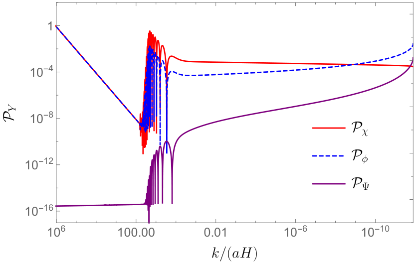
Taking Set 1 as an example, we first show the evolution of the scalar perturbations with a resonant mode. In Fig. 1, we plot the time evolution of the power spectrum at a resonant scale for each of the perturbations $\delta\chi$ , $\delta\phi$ , and $\Psi$ . This figure indicates that $\delta\phi_{k}$ exponentially grows as $\delta\chi_{k}$ exponentially grows, which is the result of the noncanonical kinetic coupling of the $\phi$ and $\chi$ fields. Meanwhile, it is easy to observe that $\delta\chi_{k}$ decays far outside the horizon due to $m_{\chi}\sim\mathcal{O}(H)$ . Moreover, it is evident that the scalar metric perturbation is a negligible source of GWs relative to the scalar fields.

Figure 2: The power spectra of the curvature perturbations obtained by setting the e-folding number from the time when the pivot scale

k_{\ast}=0.05\;{\rm Mpc}^{-1}

exits the horizon to the end of inflation as

60

. The red, blue and purple lines represent the results in Set 1, Set 2, and Set 3, respectively. The green shaded region is excluded by the CMB observations Akrami et al. 2020. The orange shaded region shows the current upper bound on the power spectrum from measurements of

\mu

distortion for COBE/FIRAS Mather et al. 1994; Fixsen et al. 1996. The forecasted constraint for the distortion experiment PIXIE Kogut et al. 2011 is shown as the orange dashed line. See Ref. Chluba et al. 2019 for the summary of constraints on the power spectrum of the curvature perturbations.

Figure 2 displays the resulting power spectrum of the curvature perturbations for these three sets of parameters. For Set 1 and Set 2, the resonant scales of the curvature perturbations are both located in the range of around $10^{12}{\rm Mpc}^{-1}$ , and the both amplitudes of the corresponding power spectra are of order $10^{-2}$ . The main difference between the two sets embodies the width of the amplified part of power spectrum due to the different field excursion $\Delta\phi$ . The power spectra of these two cases result in the production of a sizable amount of PBHs with masses around $10^{-12}M_{\odot}$ , as shown in the left panel of Fig. 3. The resulting PBHs in Set 1 and Set 2, comprising $28\%$ and $39\%$ of DM respectively, can make up of the vital component of DM. The predicted total energy spectra of GWs for Set 1 and Set 2 are plotted in the right panel of Fig. 3. It is easy to see that small $\Delta\phi$ (Set 1) and the large $\Delta\phi$ (Set 2) result in a peak and a broad plateau in the energy spectra of GWs from both the inflationary era and the radiation-dominated era, respectively. Interestingly, the height of the peak or plateau in the energy spectrum of GWs from inflation is much larger than that from the radiation-dominated era; however, the frequency of the peak or plateau in the former is located in the lower frequency range relative to that in the latter. As a result, the total energy spectrum of GWs is not dominated by the energy spectrum of GWs from inflation but displays a unique uneven double-peak or double-plateau pattern. In addition, the energy spectra of GWs from both the inflationary era and the radiation-dominated era exceed the sensitivity curves of LISA and Taiji, and the detection of such SGWBs provides us a chance to test our model.

Figure 3: The mass spectra of PBHs (left panel) and the current energy spectra of the induced GWs (right panel) for Set 1 and Set 2. The red and blue lines correspond to the results of Set 1 and Set 2, respectively. In the left panel, the lines with half shades represent the current observational constrains on PBH abundance: diffuse supernova neutrino background (SUPER-K) Dasgupta et al. 2020, extra-galactic gamma ray by the Hawking radiation (EG

\gamma

) Carr et al. 2010, galactic center 511 keV gamma-ray line (INTEGRAL) Laha 2019, and Subaru HSC microlensing (Subaru HSC) Smyth et al. 2020. In the right panel, the orange and brown dashed lines represent the sensitivity curves of the space-based projects LISA Amaro-Seoane et al. 2017 and Taiji Ruan et al. 2020, respectively.

Figure 4: The mass spectrum of PBHs (left panel) and the current energy spectra of the induced GWs (right panel) for Set 3. In the left panel, the lines with half shades show the gravitational lensing constraint from EROS/MACHO (EROS/MACHO) Tisserand et al. 2007, the constraints from GWs produced by individual mergers (Mergers) Kavanagh et al. 2018; Abbott et al. 2019 and stochastic background of mergers (SGWB) Chen and Huang 2020, and the accretion constraints (Accretion) from CMB Serpico et al. 2020, EDGES 21cm Hektor et al. 2018, X ray Manshanden et al. 2019, radio Manshanden et al. 2019, and dwarf galaxy heating Lu et al. 2021. See Refs. Carr et al. 2020; Green and Kavanagh 2021 for the summary of constraints on the abundance of PBHs. In the right panel, the gray violin plots show the five first frequency bins from the NANOGrav observation Arzoumanian et al. 2020.

For Set 3, the resonant scales of the power spectrum of the curvature perturbations approximately span from $10^{5}{\rm Mpc}^{-1}$ to $10^{7}{\rm Mpc}^{-1}$ , as seen in Fig. 2. We can see from the left panel of Fig. 4 that $f_{\rm PBH}\sim 10^{-3}$ at $M\sim\mathcal{O}(10)M_{\odot}$ , which may account for the merger rage expected by the LIGO-Virgo Collaboration Sasaki et al. 2016. We plot the energy spectra of GWs induced during the inflationary era and the radiation-dominated era compared with the five first frequency bins from NANOGrav in the right panel of Fig. 4. Obviously, the induced GWs associated with the PBH formation are compatible with the NANOGrav results. Note that in the choice of $\delta_{c}\simeq 0.45$ , the predicted GWs from the radiation-dominated era are too large to explain the NANOGrav results if we take the Gaussian or $k$ -space top-hat window function.

V Conclusions

In this work, we studied the amplification of the curvature perturbations in the single-field slow-roll inflation with a spectator scalar field kinetically coupled to the inflaton. After introducing a periodic coupling function of the inflaton, the perturbations of the spectator field at certain scales are exponentially amplified through the parametric resonance, and then the enhanced spectator field perturbations trigger the amplification of the inflaton perturbations at first-order level due to the kinetic coupling and a nonzero background of the spectator field. As a result, the curvature perturbations are enhanced to lead to the production of a sizable amount of PBHs. Meanwhile, due to ineludible second-order effect of overlarge scalar perturbations, the model leaves a sizable SGWB contributed from the inflationary era and the radiation-dominated era. Choosing the appropriate model parameters, we obtain the mass spectrum of PBHs at $\mathcal{O}(10^{-12})M_{\odot}$ as a vital component of DM. The corresponding SGWB, including two components, may be detected by the future space-based projects such as LISA and Taiji, and its energy spectrum displays unique uneven double-peak or double-plateau structure, which can be utilized to test our model. Moreover, for the case of PBHs that could explain the LIGO-Virgo events, we find that the energy spectrum of the resulting GWs originating from the radiation-dominated era is consistent with the NANOGrav signal.

Acknowledgements.

We are grateful to Jing Liu and Lang Liu for useful discussions and comments. This work is supported in part by the National Key Research and Development Program of China Grant No. 2020YFC2201501, the National Natural Science Foundation of China Grants No. 11947302, No. 11991052, No. 11690022, No. 11821505 and No. 12047559, the China Postdoctoral Science Foundation Grant No. 2020M680689, the Key Research Program of the CAS Grant No. XDPB15, and the Key Research Program of Frontier Sciences of CAS.

References

Hawking (1971) S. Hawking, Mon. Not. Roy. Astron. Soc. 152, 75 (1971).
Carr and Hawking (1974) B. J. Carr and S. W. Hawking, Mon. Not. Roy. Astron. Soc. 168, 399 (1974).
Carr (1975) B. J. Carr, Astrophys. J. 201, 1 (1975).
Belotsky et al. (2014) K. M. Belotsky, A. D. Dmitriev, E. A. Esipova, V. A. Gani, A. V. Grobov, M. Y. Khlopov, A. A. Kirillov, S. G. Rubin, and I. V. Svadkovsky, Mod. Phys. Lett. A 29, 1440005 (2014), arXiv:1410.0203 [astro-ph.CO] .
Carr et al. (2016) B. Carr, F. Kuhnel, and M. Sandstad, Phys. Rev. D 94, 083504 (2016), arXiv:1607.06077 [astro-ph.CO] .
Carr and Kuhnel (2020) B. Carr and F. Kuhnel, Ann. Rev. Nucl. Part. Sci. 70, 355 (2020), arXiv:2006.02838 [astro-ph.CO] .
Bird et al. (2016) S. Bird, I. Cholis, J. B. Muñoz, Y. Ali-Haimoud, M. Kamionkowski, E. D. Kovetz, A. Raccanelli, and A. G. Riess, Phys. Rev. Lett. 116, 201301 (2016), arXiv:1603.00464 [astro-ph.CO] .
Sasaki et al. (2016) M. Sasaki, T. Suyama, T. Tanaka, and S. Yokoyama, Phys. Rev. Lett. 117, 061101 (2016), [Erratum: Phys.Rev.Lett. 121, 059901(E) (2018)], arXiv:1603.08338 [astro-ph.CO] .
Abbott et al. (2016a) B. P. Abbott et al. (LIGO Scientific, Virgo), Phys. Rev. Lett. 116, 061102 (2016a), arXiv:1602.03837 [gr-qc] .
Abbott et al. (2016b) B. P. Abbott et al. (LIGO Scientific, Virgo), Phys. Rev. Lett. 116, 241103 (2016b), arXiv:1606.04855 [gr-qc] .
Abbott et al. (2017) B. P. Abbott et al. (LIGO Scientific, VIRGO), Phys. Rev. Lett. 118, 221101 (2017), [Erratum: Phys.Rev.Lett. 121, 129901 (2018)], arXiv:1706.01812 [gr-qc] .
Mukherjee and Silk (2021) S. Mukherjee and J. Silk, Mon. Not. Roy. Astron. Soc. 506, 3977 (2021), arXiv:2105.11139 [gr-qc] .
Mukherjee et al. (2021) S. Mukherjee, M. S. P. Meinema, and J. Silk, (2021), arXiv:2107.02181 [astro-ph.CO] .
Matarrese et al. (1998) S. Matarrese, S. Mollerach, and M. Bruni, Phys. Rev. D 58, 043504 (1998), arXiv:astro-ph/9707278 .
Noh and Hwang (2004) H. Noh and J.-c. Hwang, Phys. Rev. D 69, 104011 (2004).
Ananda et al. (2007) K. N. Ananda, C. Clarkson, and D. Wands, Phys. Rev. D 75, 123518 (2007), arXiv:gr-qc/0612013 .
Baumann et al. (2007) D. Baumann, P. J. Steinhardt, K. Takahashi, and K. Ichiki, Phys. Rev. D 76, 084019 (2007), arXiv:hep-th/0703290 .
Wang and Zhang (2017) B. Wang and Y. Zhang, Phys. Rev. D 96, 103522 (2017), arXiv:1710.06641 [gr-qc] .
Domènech and Sasaki (2018) G. Domènech and M. Sasaki, Phys. Rev. D 97, 023521 (2018), arXiv:1709.09804 [gr-qc] .
Saito and Yokoyama (2009) R. Saito and J. Yokoyama, Phys. Rev. Lett. 102, 161101 (2009), [Erratum: Phys.Rev.Lett. 107, 069901(E) (2011)], arXiv:0812.4339 [astro-ph] .
Saito and Yokoyama (2010) R. Saito and J. Yokoyama, Prog. Theor. Phys. 123, 867 (2010), [Erratum: Prog.Theor.Phys. 126, 351–352 (2011)], arXiv:0912.5317 [astro-ph.CO] .
Bugaev and Klimai (2011) E. Bugaev and P. Klimai, Phys. Rev. D 83, 083521 (2011), arXiv:1012.4697 [astro-ph.CO] .
Garcia-Bellido et al. (2017) J. Garcia-Bellido, M. Peloso, and C. Unal, JCAP 09, 013 (2017), arXiv:1707.02441 [astro-ph.CO] .
Espinosa et al. (2018) J. R. Espinosa, D. Racco, and A. Riotto, JCAP 09, 012 (2018), arXiv:1804.07732 [hep-ph] .
Kohri and Terada (2018) K. Kohri and T. Terada, Phys. Rev. D 97, 123532 (2018), arXiv:1804.08577 [gr-qc] .
Bartolo et al. (2019) N. Bartolo, V. De Luca, G. Franciolini, M. Peloso, D. Racco, and A. Riotto, Phys. Rev. D 99, 103521 (2019), arXiv:1810.12224 [astro-ph.CO] .
Cai et al. (2019a) R.-G. Cai, S. Pi, and M. Sasaki, Phys. Rev. Lett. 122, 201101 (2019a), arXiv:1810.11000 [astro-ph.CO] .
Cai et al. (2019b) Y.-F. Cai, C. Chen, X. Tong, D.-G. Wang, and S.-F. Yan, Phys. Rev. D 100, 043518 (2019b), arXiv:1902.08187 [astro-ph.CO] .
Fu et al. (2020a) C. Fu, P. Wu, and H. Yu, Phys. Rev. D 101, 023529 (2020a), arXiv:1912.05927 [astro-ph.CO] .
Cai et al. (2019c) R.-G. Cai, S. Pi, S.-J. Wang, and X.-Y. Yang, JCAP 05, 013 (2019c), arXiv:1901.10152 [astro-ph.CO] .
Pi et al. (2019) S. Pi, M. Sasaki, and Y.-l. Zhang, JCAP 06, 049 (2019), arXiv:1904.06304 [gr-qc] .
Cai et al. (2019d) R.-G. Cai, S. Pi, S.-J. Wang, and X.-Y. Yang, JCAP 10, 059 (2019d), arXiv:1907.06372 [astro-ph.CO] .
Inomata (2021) K. Inomata, JCAP 03, 013 (2021), arXiv:2008.12300 [gr-qc] .
Pi and Sasaki (2020) S. Pi and M. Sasaki, JCAP 09, 037 (2020), arXiv:2005.12306 [gr-qc] .
Braglia et al. (2020) M. Braglia, D. K. Hazra, F. Finelli, G. F. Smoot, L. Sriramkumar, and A. A. Starobinsky, JCAP 08, 001 (2020), arXiv:2005.02895 [astro-ph.CO] .
Braglia et al. (2021) M. Braglia, X. Chen, and D. K. Hazra, JCAP 03, 005 (2021), arXiv:2012.05821 [astro-ph.CO] .
Peng et al. (2021) Z.-Z. Peng, C. Fu, J. Liu, Z.-K. Guo, and R.-G. Cai, (2021), arXiv:2106.11816 [astro-ph.CO] .
Amaro-Seoane et al. (2017) P. Amaro-Seoane et al. (LISA), (2017), arXiv:1702.00786 [astro-ph.IM] .
Ruan et al. (2020) W.-H. Ruan, Z.-K. Guo, R.-G. Cai, and Y.-Z. Zhang, Int. J. Mod. Phys. A 35, 2050075 (2020), arXiv:1807.09495 [gr-qc] .
Arzoumanian et al. (2020) Z. Arzoumanian et al. (NANOGrav), Astrophys. J. Lett. 905, L34 (2020), arXiv:2009.04496 [astro-ph.HE] .
Hellings and Downs (1983) R. w. Hellings and G. s. Downs, Astrophys. J. Lett. 265, L39 (1983).
Blasi et al. (2021) S. Blasi, V. Brdar, and K. Schmitz, Phys. Rev. Lett. 126, 041305 (2021), arXiv:2009.06607 [astro-ph.CO] .
Ellis and Lewicki (2021) J. Ellis and M. Lewicki, Phys. Rev. Lett. 126, 041304 (2021), arXiv:2009.06555 [astro-ph.CO] .
Buchmuller et al. (2020) W. Buchmuller, V. Domcke, and K. Schmitz, Phys. Lett. B 811, 135914 (2020), arXiv:2009.10649 [astro-ph.CO] .
Samanta and Datta (2021) R. Samanta and S. Datta, JHEP 05, 211 (2021), arXiv:2009.13452 [hep-ph] .
Nakai et al. (2021) Y. Nakai, M. Suzuki, F. Takahashi, and M. Yamada, Phys. Lett. B 816, 136238 (2021), arXiv:2009.09754 [astro-ph.CO] .
Neronov et al. (2021) A. Neronov, A. R. Pol, C. Caprini, and D. Semikoz, Phys. Rev. D 103, L041302 (2021), arXiv:2009.14174 [astro-ph.CO] .
Bian et al. (2021) L. Bian, R.-G. Cai, J. Liu, X.-Y. Yang, and R. Zhou, Phys. Rev. D 103, L081301 (2021), arXiv:2009.13893 [astro-ph.CO] .
Abe et al. (2021) K. T. Abe, Y. Tada, and I. Ueda, JCAP 06, 048 (2021), arXiv:2010.06193 [astro-ph.CO] .
Liu et al. (2021) J. Liu, R.-G. Cai, and Z.-K. Guo, Phys. Rev. Lett. 126, 141303 (2021), arXiv:2010.03225 [astro-ph.CO] .
Vagnozzi (2021) S. Vagnozzi, Mon. Not. Roy. Astron. Soc. 502, L11 (2021), arXiv:2009.13432 [astro-ph.CO] .
Kuroyanagi et al. (2021) S. Kuroyanagi, T. Takahashi, and S. Yokoyama, JCAP 01, 071 (2021), arXiv:2011.03323 [astro-ph.CO] .
Vaskonen and Veermäe (2021) V. Vaskonen and H. Veermäe, Phys. Rev. Lett. 126, 051303 (2021), arXiv:2009.07832 [astro-ph.CO] .
De Luca et al. (2021) V. De Luca, G. Franciolini, and A. Riotto, Phys. Rev. Lett. 126, 041303 (2021), arXiv:2009.08268 [astro-ph.CO] .
Kohri and Terada (2021) K. Kohri and T. Terada, Phys. Lett. B 813, 136040 (2021), arXiv:2009.11853 [astro-ph.CO] .
Inomata et al. (2021) K. Inomata, M. Kawasaki, K. Mukaida, and T. T. Yanagida, Phys. Rev. Lett. 126, 131301 (2021), arXiv:2011.01270 [astro-ph.CO] .
Yi and Zhu (2021) Z. Yi and Z.-H. Zhu, (2021), arXiv:2105.01943 [gr-qc] .
Sugiyama et al. (2021) S. Sugiyama, V. Takhistov, E. Vitagliano, A. Kusenko, M. Sasaki, and M. Takada, Phys. Lett. B 814, 136097 (2021), arXiv:2010.02189 [astro-ph.CO] .
Domènech and Pi (2020) G. Domènech and S. Pi, (2020), arXiv:2010.03976 [astro-ph.CO] .
Akrami et al. (2020) Y. Akrami et al. (Planck), Astron. Astrophys. 641, A10 (2020), arXiv:1807.06211 [astro-ph.CO] .
Tegmark et al. (2004) M. Tegmark et al. (SDSS), Astrophys. J. 606, 702 (2004), arXiv:astro-ph/0310725 .
Garcia-Bellido and Ruiz Morales (2017) J. Garcia-Bellido and E. Ruiz Morales, Phys. Dark Univ. 18, 47 (2017), arXiv:1702.03901 [astro-ph.CO] .
Germani and Prokopec (2017) C. Germani and T. Prokopec, Phys. Dark Univ. 18, 6 (2017), arXiv:1706.04226 [astro-ph.CO] .
Motohashi and Hu (2017) H. Motohashi and W. Hu, Phys. Rev. D 96, 063503 (2017), arXiv:1706.06784 [astro-ph.CO] .
Ezquiaga et al. (2018) J. M. Ezquiaga, J. Garcia-Bellido, and E. Ruiz Morales, Phys. Lett. B 776, 345 (2018), arXiv:1705.04861 [astro-ph.CO] .
Di and Gong (2018) H. Di and Y. Gong, JCAP 07, 007 (2018), arXiv:1707.09578 [astro-ph.CO] .
Ballesteros and Taoso (2018) G. Ballesteros and M. Taoso, Phys. Rev. D 97, 023501 (2018), arXiv:1709.05565 [hep-ph] .
Dalianis et al. (2019) I. Dalianis, A. Kehagias, and G. Tringas, JCAP 01, 037 (2019), arXiv:1805.09483 [astro-ph.CO] .
Gao and Guo (2018) T.-J. Gao and Z.-K. Guo, Phys. Rev. D 98, 063526 (2018), arXiv:1806.09320 [hep-ph] .
Drees and Xu (2021) M. Drees and Y. Xu, Eur. Phys. J. C 81, 182 (2021), arXiv:1905.13581 [hep-ph] .
Xu et al. (2020) W.-T. Xu, J. Liu, T.-J. Gao, and Z.-K. Guo, Phys. Rev. D 101, 023505 (2020), arXiv:1907.05213 [astro-ph.CO] .
Fu et al. (2019) C. Fu, P. Wu, and H. Yu, Phys. Rev. D 100, 063532 (2019), arXiv:1907.05042 [astro-ph.CO] .
Lin et al. (2020) J. Lin, Q. Gao, Y. Gong, Y. Lu, C. Zhang, and F. Zhang, Phys. Rev. D 101, 103515 (2020), arXiv:2001.05909 [gr-qc] .
Fu et al. (2020b) C. Fu, P. Wu, and H. Yu, Phys. Rev. D 102, 043527 (2020b), arXiv:2006.03768 [astro-ph.CO] .
Yi et al. (2021) Z. Yi, Q. Gao, Y. Gong, and Z.-h. Zhu, Phys. Rev. D 103, 063534 (2021), arXiv:2011.10606 [astro-ph.CO] .
Ballesteros et al. (2019) G. Ballesteros, J. Beltran Jimenez, and M. Pieroni, JCAP 06, 016 (2019), arXiv:1811.03065 [astro-ph.CO] .
Kamenshchik et al. (2019) A. Y. Kamenshchik, A. Tronconi, T. Vardanyan, and G. Venturi, Phys. Lett. B 791, 201 (2019), arXiv:1812.02547 [gr-qc] .
Cai et al. (2018) Y.-F. Cai, X. Tong, D.-G. Wang, and S.-F. Yan, Phys. Rev. Lett. 121, 081306 (2018), arXiv:1805.03639 [astro-ph.CO] .
Chen and Cai (2019) C. Chen and Y.-F. Cai, JCAP 10, 068 (2019), arXiv:1908.03942 [astro-ph.CO] .
Chen et al. (2020) C. Chen, X.-H. Ma, and Y.-F. Cai, Phys. Rev. D 102, 063526 (2020), arXiv:2003.03821 [astro-ph.CO] .
Cai et al. (2020) R.-G. Cai, Z.-K. Guo, J. Liu, L. Liu, and X.-Y. Yang, JCAP 06, 013 (2020), arXiv:1912.10437 [astro-ph.CO] .
Zhou et al. (2020) Z. Zhou, J. Jiang, Y.-F. Cai, M. Sasaki, and S. Pi, Phys. Rev. D 102, 103527 (2020), arXiv:2010.03537 [astro-ph.CO] .
Liu and Xu (2021) L.-H. Liu and W.-L. Xu, (2021), arXiv:2107.07310 [astro-ph.CO] .
Ashoorioon et al. (2021) A. Ashoorioon, A. Rostami, and J. T. Firouzjaee, JHEP 07, 087 (2021), arXiv:1912.13326 [astro-ph.CO] .
Cheng et al. (2018) S.-L. Cheng, W. Lee, and K.-W. Ng, JCAP 07, 001 (2018), arXiv:1801.09050 [astro-ph.CO] .
Özsoy and Lalak (2021) O. Özsoy and Z. Lalak, JCAP 01, 040 (2021), arXiv:2008.07549 [astro-ph.CO] .
Cook and Sorbo (2012) J. L. Cook and L. Sorbo, Phys. Rev. D 85, 023534 (2012), [Erratum: Phys.Rev.D 86, 069901(E) (2012)], arXiv:1109.0022 [astro-ph.CO] .
Goolsby-Cole and Sorbo (2017) C. Goolsby-Cole and L. Sorbo, JCAP 08, 005 (2017), arXiv:1705.03755 [astro-ph.CO] .
Biagetti et al. (2013) M. Biagetti, M. Fasiello, and A. Riotto, Phys. Rev. D 88, 103518 (2013), arXiv:1305.7241 [astro-ph.CO] .
Biagetti et al. (2015) M. Biagetti, E. Dimastrogiovanni, M. Fasiello, and M. Peloso, JCAP 04, 011 (2015), arXiv:1411.3029 [astro-ph.CO] .
Fujita et al. (2015) T. Fujita, J. Yokoyama, and S. Yokoyama, PTEP 2015, 43E01 (2015), arXiv:1411.3658 [astro-ph.CO] .
Starobinsky et al. (2001) A. A. Starobinsky, S. Tsujikawa, and J. Yokoyama, Nucl. Phys. B 610, 383 (2001), arXiv:astro-ph/0107555 .
Domènech and Sasaki (2021) G. Domènech and M. Sasaki, Phys. Rev. D 103, 063531 (2021), arXiv:2012.14016 [gr-qc] .
van de Bruck and Robinson (2014) C. van de Bruck and M. Robinson, JCAP 08, 024 (2014), arXiv:1404.7806 [astro-ph.CO] .
Gordon et al. (2000) C. Gordon, D. Wands, B. A. Bassett, and R. Maartens, Phys. Rev. D 63, 023506 (2000), arXiv:astro-ph/0009131 .
Ando et al. (2018) K. Ando, K. Inomata, and M. Kawasaki, Phys. Rev. D 97, 103528 (2018), arXiv:1802.06393 [astro-ph.CO] .
Musco et al. (2005) I. Musco, J. C. Miller, and L. Rezzolla, Class. Quant. Grav. 22, 1405 (2005), arXiv:gr-qc/0412063 .
Blais et al. (2003) D. Blais, T. Bringmann, C. Kiefer, and D. Polarski, Phys. Rev. D 67, 024024 (2003), arXiv:astro-ph/0206262 .
Josan et al. (2009) A. S. Josan, A. M. Green, and K. A. Malik, Phys. Rev. D 79, 103520 (2009), arXiv:0903.3184 [astro-ph.CO] .
Sasaki et al. (2018) M. Sasaki, T. Suyama, T. Tanaka, and S. Yokoyama, Class. Quant. Grav. 35, 063001 (2018), arXiv:1801.05235 [astro-ph.CO] .
Zhao and Zhang (2006) W. Zhao and Y. Zhang, Phys. Rev. D 74, 043503 (2006), arXiv:astro-ph/0604458 .
Mather et al. (1994) J. C. Mather et al., Astrophys. J. 420, 439 (1994).
Fixsen et al. (1996) D. J. Fixsen, E. S. Cheng, J. M. Gales, J. C. Mather, R. A. Shafer, and E. L. Wright, Astrophys. J. 473, 576 (1996), arXiv:astro-ph/9605054 .
Kogut et al. (2011) A. Kogut et al., JCAP 07, 025 (2011), arXiv:1105.2044 [astro-ph.CO] .
Chluba et al. (2019) J. Chluba et al., (2019), 10.1007/s10686-021-09729-5, arXiv:1909.01593 [astro-ph.CO] .
Dasgupta et al. (2020) B. Dasgupta, R. Laha, and A. Ray, Phys. Rev. Lett. 125, 101101 (2020), arXiv:1912.01014 [hep-ph] .
Carr et al. (2010) B. J. Carr, K. Kohri, Y. Sendouda, and J. Yokoyama, Phys. Rev. D 81, 104019 (2010), arXiv:0912.5297 [astro-ph.CO] .
Laha (2019) R. Laha, Phys. Rev. Lett. 123, 251101 (2019), arXiv:1906.09994 [astro-ph.HE] .
Smyth et al. (2020) N. Smyth, S. Profumo, S. English, T. Jeltema, K. McKinnon, and P. Guhathakurta, Phys. Rev. D 101, 063005 (2020), arXiv:1910.01285 [astro-ph.CO] .
Tisserand et al. (2007) P. Tisserand et al. (EROS-2), Astron. Astrophys. 469, 387 (2007), arXiv:astro-ph/0607207 .
Kavanagh et al. (2018) B. J. Kavanagh, D. Gaggero, and G. Bertone, Phys. Rev. D 98, 023536 (2018), arXiv:1805.09034 [astro-ph.CO] .
Abbott et al. (2019) B. P. Abbott et al. (LIGO Scientific, Virgo), Phys. Rev. Lett. 123, 161102 (2019), arXiv:1904.08976 [astro-ph.CO] .
Chen and Huang (2020) Z.-C. Chen and Q.-G. Huang, JCAP 08, 039 (2020), arXiv:1904.02396 [astro-ph.CO] .
Serpico et al. (2020) P. D. Serpico, V. Poulin, D. Inman, and K. Kohri, Phys. Rev. Res. 2, 023204 (2020), arXiv:2002.10771 [astro-ph.CO] .
Hektor et al. (2018) A. Hektor, G. Hütsi, L. Marzola, M. Raidal, V. Vaskonen, and H. Veermäe, Phys. Rev. D 98, 023503 (2018), arXiv:1803.09697 [astro-ph.CO] .
Manshanden et al. (2019) J. Manshanden, D. Gaggero, G. Bertone, R. M. T. Connors, and M. Ricotti, JCAP 06, 026 (2019), arXiv:1812.07967 [astro-ph.HE] .
Lu et al. (2021) P. Lu, V. Takhistov, G. B. Gelmini, K. Hayashi, Y. Inoue, and A. Kusenko, Astrophys. J. Lett. 908, L23 (2021), arXiv:2007.02213 [astro-ph.CO] .
Carr et al. (2020) B. Carr, K. Kohri, Y. Sendouda, and J. Yokoyama, (2020), arXiv:2002.12778 [astro-ph.CO] .
Green and Kavanagh (2021) A. M. Green and B. J. Kavanagh, J. Phys. G 48, 043001 (2021), arXiv:2007.10722 [astro-ph.CO] .