Culling the Herd of Moments with Penalized Empirical Likelihood
Abstract
Models defined by moment conditions are at the center of structural econometric estimation, but economic theory is mostly agnostic about moment selection. While a large pool of valid moments can potentially improve estimation efficiency, in the meantime a few invalid ones may undermine consistency. This paper investigates the empirical likelihood estimation of these moment-defined models in high-dimensional settings. We propose a penalized empirical likelihood (PEL) estimation and establish its oracle property with consistent detection of invalid moments. The PEL estimator is asymptotically normally distributed, and a projected PEL procedure further eliminates its asymptotic bias and provides more accurate normal approximation to the finite sample behavior. Simulation exercises demonstrate excellent numerical performance of these methods in estimation and inference.
Keywords: Empirical likelihood; Estimating equations; High-dimensional statistical methods; Misspecification; Moment selection; Penalized likelihood
1 Introduction
Economists’ perennial pursuit of structural mechanisms leads to models defined by moments. These models can be written in a semiparametric form where is a vector of estimating functions, is a vector of unknown parameters, and is observed data. To estimate these models, the most popular method is generalized method of moments (GMM) (Hansen 1982). Empirical likelihood (EL) (Qin and Lawless 1994) is a competitive alternative to GMM, thanks to its nice statistical properties. Both GMM and EL are essential building blocks of modern econometrics (Anatolyev and Gospodinov 2011).
Ideally, economists count on economic theory to guide the choice of variables and moments. However, the truth is that most economic theories are parsimonious abstractions and rarely pinpoint these choices in data-rich environments. The indeterminacy of moment selection brings about three related issues. The first is weak moments (Stock et al. 2014), which threatens identification of the true value when multiple ’s satisfy . Practitioners respond to the concerns of weak moments by adding more moment conditions in the hope to strengthen identification, causing the second issue of many moments (Roodman 2009). The hazard of many moments is the possible inclusion of invalid moments, meaning for some (Murray 2006), which is the third issue. These cited survey papers highlight the unease incurred by the three challenges and econometricians’ efforts in coping with them.
When an underlying economic theory is ambivalent, empirical results based on it can be controversial and susceptible to cherry-picking. In such a circumstance, of great importance are data-driven methods to guide and discipline moment selection. In the low-dimensional settings, Andrews and Lu 2001 propose the GMM information criteria, and Hong et al. 2003 follow with the counterpart for EL. Information criteria are evaluated exhaustively at all combinations of moments, and the computation becomes infeasible when there are many potential moments. To overcome this challenge, Liao 2013 ushers the adaptive Lasso shrinkage into GMM to select among a finite number of moments, and Cheng and Liao 2015 further extend it to deal with a diverging number of moments and accommodate invalid ones.
Unprecedented progress in computation and information technology fuel an arms race between the sheer size of the data and the scale of empirical models. In the era of big data, on the one hand the cost of data collection and processing is tremendously lowered and rich datasets open new perspectives to inspect a myriad of problems; on the other hand economists attempt to build general models to capture various sources of heterogeneity in observational data. Empirical applications abound with models of many potential moments. For instance, Eaton et al. 2011 create 1360 moments to estimate a structural trade model, Altonji et al. 2013 match 2429 moments implied by a model of earning dynamics, and early works of linear instrumental variables (IV) models produce thousands of instruments by interacting variables (Angrist and Krueger 1992). Although the sample sizes in these examples are non-trivial, the proliferation of moments calls for a moment selection procedure capable of handling high-dimensional moments at a magnitude unrestricted by the sample size. In particular, invalid ones that jeopardize consistency must be identified and “culled” from the herd of moments.
The quadratic form of the usual GMM criterion function is incompatible with high-dimensional moments (Shi 2016a, Shi 2016b), and thus Belloni et al. 2018 regularize GMM with the sup-norm. In this paper, we contribute the most general and versatile procedure for high-dimensional nonlinear settings, to the best of our knowledge. We first develop a penalized empirical likelihood (PEL) solution (Chang et al. 2018) to deal with valid and invalid moments simultaneously. We neutralize the invalid moments by an auxiliary parameter, following Liao 2013 and Cheng and Liao 2015. We establish the rate of convergence and asymptotic normality of the PEL estimator, and show the efficiency gain from incorporating extra valid moments. Under suitable conditions, it transpires that PEL enjoys the oracle property of consistent moment selection and parameter selection.
The asymptotic normal distribution of the PEL estimator involves a bias term caused by the high-dimensional moments. To spare the estimation of the bias term, we can take further actions to project out the influence of the high-dimensional nuisance parameter in the PEL estimator, which is called projected PEL (PPEL) (Chang et al. 2021). The asymptotic normality of the PPEL estimator is free of bias, which facilitates statistical inference of the structural parameter as well as the validity of moments. Invoking statistical learning to assist our decisions, our method fits well in the recent trend of machine learning for the automatic selection of moments and variables.
Although this paper follows Chang et al. 2018 for estimation and Chang et al. 2021 for inference procedures, the key insight lies in the observations that the high-dimensional auxiliary parameter, which signifies the magnitude of misspecification, can be incorporated in the EL method as an additional high-dimensional parameter. In this paper, “high-dimensional” means that the numbers of parameters and/or moments are larger than the sample size, which goes beyond the scope of Liao 2013 and Cheng and Liao 2015. On the other hand, in order to adapt Chang et al. 2018 and Chang et al. 2021 to accommodate misspecified moments, we must deal with the distinctive roles of the main parameter of interest and the auxiliary parameter in identification and the technical challenges induced by them. Differences from Chang et al. 2018 are highlighted in Section 3 about the rates of converges of the two components of the parameters, and those from Chang et al. 2021 are elaborated in Section 5 about the ways of confidence region construction.
Literature review. Our paper stands on strands of literature, which are too vast to survey exhaustively. The accumulation of moments started from the linear IV model (Angrist 1990, Angrist and Keueger 1991). The linear IV model motivates theoretical research on issues of many IV (Bekker 1994), weak IV (Stock and Yogo 2005, Andrews and Cheng 2012), many weak IV (Chao et al. 2011, Hansen and Kozbur 2014), invalid moments and many invalid IV (Kolesár et al. 2015, Windmeijer et al. 2019), to name a few. In high-dimensional contexts, Belloni et al. 2012 use Lasso method for IV selection in the first stage, and Belloni et al. 2014 deal with post-selection inference. Utilizing the linear structure, Gold et al. 2020 and Caner and Kock 2018 provide inferential procedures for low-dimensional parameters in models with high-dimensional endogenous variables and high-dimensional IVs. Our method includes the linear IV model as a special case. In particular, the case of high-dimensional structural parameters is elaborated in Section 4.
The proliferation of moments spreads from linear IV models to nonlinear models. For example, in empirical industrial organization researchers bring in moments from various resources, some of which are guided by economic theory, to mitigate the concerns of weak identification and improve estimation efficiency (Ackerberg et al. 2007). In empirical macroeconomics, identification failure and moment misspecification are common issues (Mavroeidis 2005). Under the GMM framework, inference under weak moments (Stock and Wright 2000, Kleibergen 2005, Andrews and Mikusheva 2020), estimation under many weak moments (Han and Phillips 2006), and robust procedures for invalid moments (DiTraglia 2016, Caner et al. 2018) have been developed.
EL’s attractive theoretical properties are studied extensively (Kitamura 2001, Otsu 2010, Matsushita and Otsu 2013, Chang et al. 2015). Otsu 2006 and Newey and Windmeijer 2009 deal with its inference under weak IV, and Caner and Fan 2015 select instruments in linear IV models. Penalization schemes on EL have been introduced by Otsu 2007, Tang and Leng 2010 and Chang et al. 2018.
Organization. The rest of the paper is organized as follows. Section 2 introduces the model and the analytic framework. We first derive the asymptotic properties of our estimation in the low-dimensional case in Section 3, extend them to the high-dimensional structural parameter in Section 4, and we further refine PEL with projection to eliminate its bias in Section 5. The theoretical results are supported in Section 6 by Monte Carlo simulations. The influential study of the determinants of economic outcomes after colonialism is revisited in Section 7. Section 8 concludes the paper. Due to the limitations of space, the proofs and the technical details of secondary importance are relegated into the supplementary materials.
Notations. We conclude Introduction with notations used throughout the paper. “Low-dimensional” is referred to the cases that the number of parameters or moments is much smaller than the sample size , whereas “high-dimensional” goes the opposite. For two sequences of positive numbers and , we write or if there exists a positive constant such that , and write or if .
Denote by the indicator function. For a positive integer , we write . For a symmetric matrix , denote by and the smallest and largest eigenvalues of , respectively. For a matrix , let be its transpose, , for any , be the sup-norm, and be the spectral norm. Specifically, if , we use , and to denote the -norm, -norm and -norm of the -dimensional vector , respectively. For two square matrices and , we say if is a positive semi-definite matrix.
The population mean is denoted by , and the sample mean by . For a given index set , let be its cardinality. For a generic multivariate function , we denote by the subvector of collecting the components indexed by . Analogously, we write as the corresponding subvector of . For simplicity and when no confusion arises, we use the generic notation as the equivalence to , and for the first-order partial derivative of with respect to . Denote by the -th component of , and by the second derivative of with respect to . Let , and write its -th component as . Analogously, let and .
2 Empirical likelihood with a herd of moments
In this section we introduce the model and the EL estimation. Let be -dimensional independent and identically distributed generic observations, and be a -dimensional parameter taking values in . For a set of estimating functions , the information of the model parameter is collected by the unbiased moment condition
| (2.1) |
at the unknown true parameter , where is necessary for identifying . The superscript labels this initial set, to be distinguished from the other set in Section 2.2.
2.1 EL estimation with valid moments
Motivated from empirical applications in asset pricing, the two-step GMM (Hansen 1982) was the default estimating method for the moment-defined model (2.1). Intensive theoretical studies and numerical evidence in 1980’s and 90’s revealed some undesirable finite-sample properties of the two-step GMM (Altonji and Segal 1996). EL and the continuously updating GMM (CUE) (Hansen et al. 1996) emerged as competitive solutions, and they were later unified as members of generalized empirical likelihood (Newey and Smith 2003).
This paper focuses on EL with estimating equations:
proposed by Qin and Lawless 1994 based on the seminal idea of EL (Owen 1988, Owen 1990). Maximizing with respect to delivers the EL estimator , which can be carried out equivalently by solving the corresponding dual problem
| (2.2) |
where and is an open interval containing zero.
To fix ideas, we first study the asymptotic property of under regularity conditions. When the sample size grows, we adopt the asymptotic framework of Hjort et al. 2009 and Chang et al. 2015 to take the observations as a multi-index array, where , and may depend on . Proposition A.1 in the supplementary materials shows that the standard asymptotic normality for holds under mild regularity conditions.
2.2 Oracle EL estimation
In applied econometrics, there has been a tendency of assembling many IVs or creating many moments to identify the parameter of interest. In these applications, researchers often have some ideas about the relative importance of moments; in the meantime, when researchers work with more and more moments, some invalid ones may creep in.
Example 1.
Eaton et al. 2011 deem as the key moments 128() combinations of the largest 7 trade partners of France, which are more important than the other 1232 moments. Angrist 1990 treats the date of birth (DOB) as the key IV and it is complemented by the IVs generated by interactions; recently Kolesár et al. 2015 raise the potential invalidity among these interaction terms.11 1 Identification of the simple linear IV model requires the IVs satisfying the orthogonality condition and the relevance condition. However, the more relevant an IV to the endogenous variables, the more likely it is that the so-called “IV” is correlated with the structural error, thereby violating orthogonality. There is a thin line between a valid IV and an invalid one.
To put into an analytic framework a herd of extra moments with unknown validity ex ante, suppose that estimating functions are partitioned into two groups:
Here the estimating functions in the set are correctly specified, which can help improve the efficiency in estimating . On the contrary, those in are misspecified, and they can only undermine the identification of .
If there is an “oracle” that reveals which components of belong to , i.e., the valid estimating functions, we can collect all valid estimating functions indexed by to estimate . Denote and as the total number of valid moments. The associated EL estimation for based on the estimating functions is given by
where . By the same arguments as those in Proposition A.1 in the supplementary materials, the following Proposition 2.1 verifies the asymptotic normality for .
Proposition 2.1 (Oracle property).
Assume that satisfies the conditions (A.1)–(A.5) in the supplementary materials associated with . If and , then as for any with , where with .
Obviously is more efficient than thanks for the additional moment restrictions in , which disclose more information about the parameter and thus tie down the estimation variability. This is parallel to Hall et al. 2007 in GMM for finite numbers of parameters and moments. In reality, however, we are oblivious to , and therefore we cannot blindly summon all estimating functions in to estimate . Following Liao 2013, we introduce an auxiliary parameter to neutralize the misspecified moments. Denote the augmented parameter , and the augmented parameter space . Let and stack these estimating functions as . Then with can be identified by
| (2.3) |
Can we directly include the auxiliary parameter into the EL estimation? The answer is negative. If the auxiliary parameter is not regularized, the EL estimators with and without are the same, up to numerical errors.
Proposition 2.2.
If is the unique solution of (2.2), then , where is the associated subvector of for the estimation of with .
Proposition 2.2 states the equivalence between and . In the next section, we will show that desirable efficiency as in the oracle estimator can be achieved if we extend Liao 2013’s idea of shrinking the auxiliary parameter22 2 In GMM estimation under a fixed , Liao 2013 shrinks toward zero using the adaptive Lasso (Zou 2006). by further penalizing the Lagrange multipliers associated with the high-dimensional moments.
3 High-dimensional moments with low-dimensional
We consider in this section the model (2.3) with a low-dimensional parameter , low-dimensional estimating functions and high-dimensional estimating functions . In this setting, and are either fixed or diverge at some slow polynomial rates of , whereas can grow much larger than . The components in the parameter are indexed by . All moments together are indexed by , in which the researcher knows that those in are correctly specified in the sense that , whereas she is uncertain whether those in satisfy or not. As there is a one-to-one relationship between and the uncertain moments, we use to index the components in as well.
We propose the following PEL to simultaneously estimate the unknown parameter and determine the validity of the estimating functions in :
| (3.1) |
where , and and are two penalty functions with tuning parameters and , respectively. With the penalty function and appropriately selected tuning parameter , the estimator is associated with a sparse Lagrange multiplier . Since the sparse invokes a subset of the estimating functions , it digests the high-dimensional moments as long as the number of nonzero components in is small. On the other hand, the penalty is applied to identify which components in are correctly specified and can estimate exactly as with high probability.
These penalties originally appeared in Chang et al. 2018 though, there are several important differences. First, given the low-dimensional , it is unnecessary to assume sparsity on for identification. As a result, our procedure here in (3.1) only penalizes and , not the entire parameter and the associated Lagrange multiplier . Were penalized, we would rule out some components of and thus may suffer loss of estimation efficiency for . Second, the identification condition invoked in this paper deviates from that in Chang et al. 2018. Our Condition 1 for identification is imposed on , rather than the whole parameter . In contrast, Chang et al. 2018 specify identification condition for the parameter entity. While estimators in Chang et al. 2018 share the same rate of convergence, we must deal with the disparate rates of convergence of the main component and the auxiliary , which significantly complicates the theoretical analysis of (3.1), as detailed in Proposition 3.1 below.
For any penalty function with a tuning parameter , let for any and . We assume that the two penalty functions and involved in (3.1) belong to the following class:
| (3.2) |
This class , considered in Lv and Fan 2009, is broad and general. The commonly used penalty, SCAD penalty (Fan and Li 2001) and MCP penalty (Zhang 2010) are all included in . When , we write the associated as for simplification.
To establish the limiting distribution of in (3.1), we assume the following regularity conditions.
Condition 1.
There exists a universal constant such that
for any .
Condition 2.
There exist universal constants and such that
Condition 3.
For each , the function is twice continuously differentiable with respect to for any . For specified in Condition 2,
There is some universal constant such that .
For any index set and , define . When , we write for conciseness.
Condition 4.
There exists a universal constant such that .
Conditions 1–4 are standard regularity assumptions in the literature. Condition 1 is an identification assumption of the estimating equations in the known set . Write , and we continue by defining
| (3.3) |
in this section, where . Suppose:
| There exist and with such that | (3.4) |
to control the bias induced by on . With the assumption that the nonzero components of do not diminish to zero too fast, (3.4) can be replaced by
| (3.5) |
for some constant . If we select as an asymptotically unbiased penalty such as SCAD or MCP, we have in (3.5) when
| (3.6) |
To simplify the presentation, in this section we assume that (3.6) holds and in (3.5).33 3 If (3.6) is violated, the asymptotic normality of in Theorem 3.1 below will still hold under (3.4) along with more complicated notations to spell out the restrictions.
To allocate the parameter of interest and those invalid moments in , we define an index set and its cardinality . For any , the set picks out . Since , the corresponding auxiliary coefficients can be written as and furthermore as is the set of valid moments. Given some constant , define with . We assume the existence of a sequence such that
with some .
Let and . Then . Define for some fixed . Consider
| (3.7) |
Proposition 3.1 shows that such a is a sparse local minimizer for (3.1).
Proposition 3.1.
Let for defined in (3.2), and be convex with bounded second derivative around . For defined as (3.7), assume there exists a constant such that . Under Conditions 1–4 and (3.6), if , , , and , then with probability approaching one this provides a sparse local minimizer for the nonconvex optimization (3.1) such that (i) , (ii) , and (iii) as .
In the rest of this section, we focus on the sparse local minimizer specified in (3.7). We proceed with additional regularity conditions.
Condition 5.
There exists a universal constant such that for any with , where .
Condition 5 is the sparse Riesz condition (Zhang and Huang 2008, Chen and Chen 2008) in our setting to deal with the high-dimensional when . Let be the vector of Lagrange multiplier defined at :
Write and . Let be the set of the estimated binding moments. Since only those ’s associated with are penalized, it follows that
For any unbinding moment , define
| (3.8) |
If for some , the subdifferential at has to include the zero element (Bertsekas 1997). That is, for any . In our theoretical analysis, we impose the next condition.
Condition 6.
as .
Remark 3.1.
Condition 6 requires that does not lie on the boundary with probability approaching one, which is realistic in practice. If the distribution function of is continuous at , we then have . Condition 6 makes sure that is continuously differentiable at with probability approaching one. See Lemma A.5 in the supplementary materials.
Define and . Let , and then can be decomposed into two disjoint parts and . Furthermore, we define . The fact implies that . For any , we have . Define
with , and , where , with for , for with , and specified in (3.8) for . The limiting distribution of is stated in Theorem 3.1.
Theorem 3.1.
Remark 3.2.
Notice that . To satisfy the restrictions in Theorem 3.1, it is sufficient for to have: , , , the tuning parameters and satisfying , and .
Thanks to the extra valid moments in , the asymptotic covariance of is smaller than that of which utilizes the information in only. On the other hand, given that provides asymptotic normality under the set of correctly specified moments , one may question whether it is worthwhile to consider all the available moments among which some may risk misspecification. This is a trade-off between robustness and efficiency, a recurrent theme in modern econometrics. Although it inevitably depends on the data generating process (DGP), in big data environments the efficiency gain may be substantial. Benefits are demonstrated in the simulation exercises and the empirical application via very simple econometric models.44 4 See the RMSEs in Table 2, the length of confidence intervals in Figure 2, and the standard deviations in Table 4.
Remark 3.3.
The setting with the sets and is the same as Liao 2013. When estimating (2.3) with low-dimensional moments based on GMM, Cheng and Liao 2015 require the number of estimating functions , and the signal of invalid estimating functions . Our conditions on the relative size of the dimensions are more general. A sufficient condition for (3.6) is , in view of . Under the restrictions discussed in Remark 3.2, if we select and sufficiently close to and , respectively, then (3.6) holds provided that . This is similar to the “beta-min condition” which is necessary for consistent variable selection by shrinkage methods (Bühlmann 2013).
Remark 3.4.
Under low-dimensional moments the asymptotic normality involves no bias; see Liao 2013 and Cheng and Liao 2015. In contrast, Theorem 3.1 here makes clear that the high-dimensional moments incur an additional asymptotic bias . To conduct hypothesis testing or construct confidence region about , in principle we can estimate and correct the bias . Such a direct bias correction approach, nevertheless, is undesirable in practice and in theory. The bias term involves multiplication and inverse of large matrices, which are difficult to estimate with precision in finite samples. Illustrated in our simulation experiments in Section 6, we are unsatisfied with the asymptotic normality approximation after estimating and correcting the bias. Thus, we view Theorem 3.1 as a characterization of the asymptotic behavior of , but we do not encourage carrying out statistical inference based on it. Instead, Section 5 recommends PPEL for inference.
While the augmented parameter essentially validates all moments in , the efficiency gain comes from the penalty on that shrinks some , , to zero, thereby confirming the validity of these associated moments. To discuss moment selection, we write . If all valid estimating functions in are selected by the optimization (3.1), i.e., for all , then the asymptotic covariance of is .
Remind that in Proposition 2.1 is the semiparametric efficiency bound for the estimation of under the oracle, and Proposition 3.1 shows that as , which provides a natural moment selection criterion
| (3.9) |
to identify the valid estimating functions in . Notice that Proposition 3.1 also indicates that . Together with (3.6), we have as . Based on these arguments, Theorem 3.2 supports our proposed moments selection criterion.
Theorem 3.2.
Under the conditions of Proposition 3.1, it holds that as .
Up to now, we have established the asymptotic properties of the PEL estimator for the moment-defined model (2.3) with high-dimensional moments and low-dimensional . The next section further extends the estimation to a high-dimensional structural parameter.
4 High-dimensional moments with high-dimensional
A high-dimensional parameter is present when many control variables are included in the structural model. For example, the leading case of the linear IV model takes only one endogenous variable and it is accompanied by a few corresponding IVs. Nevertheless, such a simple setting may still involve many exogenous control variables in the main equation, and these control variables are natural instruments for themselves. An empirical example can be found in Blundell et al. 1993. Fan and Liao 2014 propose the focused GMM for such a linear IV model, which is a special case of the moment-defined model.
In this section, and are both allowed to be much larger than , whereas is fixed or diverges at some slow polynomial rate of . We assume sparse in the sense that most of its components are zero. Write and define the active set with cardinality . To obtain a sparse estimate of , we add to (3.1) a penalty on to produce the following optimization problem:
| (4.1) |
With slight abuse of notation, we keep using to denote the solution to (4.1).
As can be bigger than in high dimension, here we update Condition 1 for the identification of . In view of Chang et al. 2018, we impose Condition 1′ below for the identification of the nonzero components of .
Condition 1′.
(i) There exists a universal constant such that
for any . (ii) There exists a universal constant such that .
As we have shown in Section 3, the index set and the quantities and play key roles in the theoretical analysis of the low-dimensional in (3.1). Under the current high-dimensional setting, we define
| (4.2) |
This indexes all nonzero components in the true augmented parameter . Compared to its counterpart in Section 3, the newly defined here is amended with an extra term due to the penalty imposed on . In the current high-dimensional setting, we also redefine
| (4.3) |
with in (4.2). To control the bias introduced by on and , similar to (3.6), we assume that among the elements in , the minimal active signal is
| (4.4) |
with in (4.3) and for some constant .55 5 See the arguments below (3.5) for the validity of these assumptions. Given the newly defined and , we can further update , , , and in the same manner as their counterparts in Section 3. Moreover, we also define and as specified in Section 3 with . For any , we have .
Proposition A.2 in the supplementary materials shows that there exists a sparse local minimizer for the nonconvex optimization (4.1) such that as , which means all zero components of can be estimated exactly as zero with high probability. The limiting distribution of such and the moment selection outcomes are stated in Theorem 4.1 below.
Theorem 4.1.
Let for defined in (3.2), and be convex with bounded second derivative around . For the sparse local minimizer for (4.1) specified in Proposition A.2 in the supplementary materials, assume there exists a constant such that . Suppose Conditions 1′, 2–4 and (4.4) hold. Furthermore, assume Condition 5 holds with the newly defined , replacing by and replacing by , and Condition 6 holds with the newly defined . If , , , and , then we have
for any with as , where is the first components of , are given by (4.2) and (4.3), respectively, and with . Moreover, under the conditions of Proposition A.2 in the supplementary materials, it holds that as , where is specified in (3.9).
Remark 4.1.
Compared to (3.1), a penalty on is added to (4.1). To appreciate the benefit from this additional penalty on the sparse parameter, without loss of generality, we write and the inverse of in Theorem 3.1 in the following compatible partitioned matrix
where is a matrix. The asymptotic covariance of by (3.1) is , and that in (4.1) is according to Theorem 4.1. Notice that by the inverse of a partitioned matrix. Implicitly restricting the parameter space, the penalty on gains efficiency for the estimation of , the nonzero components of .
Remark 4.2.
Theorem 4.1 spells out the limiting distribution and efficiency gain for the estimator of the nonzero components in . If one is interested in some coefficient in , we have consistency in that as , but the limiting distribution is irregular due to the shrinkage.66 6 This is a generic property shared by procedures of the oracle properties, for example SCAD (Fan and Li 2001) and the adaptive Lasso (Zou 2006). Furthermore, parallel to Theorem 3.1 the asymptotic bias is again present. Similar to Remark 3.4, we do not suggest conducting statistical inference predicated on this characterization of the asymptotic behavior of normality.
Statistical inference is important in applied econometrics when researchers intend to assess whether the estimated result supports or rejects a hypothesized value of the parameter. The next section proposes an inferential procedure based on a projection of estimating functions, which is free of asymptotic biases.
5 Confidence regions for a subset of
Suppose we are interested in the inference for a subset of parameters for some generic small subset with . Here we allow to be fixed or diverge slowly with the sample size . What is novel here is that is allowed to contain part of the auxiliary parameter , for which our method will provide a formal statistical inference for the validity of a subset of the high-dimensional moment restrictions. In contrast, Liao 2013 offers asymptotic normality for the structural parameter under low-dimensional moments but does not characterize the asymptotic distribution of the auxiliary parameter .
A key technical issue is how to deal with the high-dimensional nuisance parameter , where . Our approach follows Chang et al. 2021 to project out the influence of the nuisance parameter. Such idea was also used in Ning and Liu 2017 and Neykov et al. 2018. Given an initial estimate for , we first determine a linear transformation matrix with each row defined as
| (5.1) |
for , where as is a tuning parameter, and is a basis of the linear space . In practice, we can specify the -dimensional vector with all zero elements except one unit entry. As we will discuss in Remark 5.2, the solution from (3.1) or (4.1) can serve as the initial estimator .
Based on as in (5.1), we then obtain the new -dimensional estimating functions by projecting on :
Write and define an matrix . The definition of implies that . Since all the components in the -th column of are zero for , the newly defined estimating functions is uninformative of the nuisance parameter . Informative is of the parameter of interest, as for some components in the -th column of must be nonzero.
Given the projected estimating functions , it is possible to directly borrow from Chang et al. 2021 to construct the confidence region of by the EL ratio
with respect to , where . Since as for a fixed , the set provides a confidence region for , where is the -quantile of distribution. Nonetheless, the finite-sample performance of such an asymptotically valid confidence region depends crucially on the convexity of near . If convexity fails in a finite sample, this EL-ratio-based confidence region will be voluminous in magnitude due to numerical instability. Verifying the convexity condition is onerous, in particular when is large, for may be a nonlinear function of .
To secure a stable confidence region for , in this paper we deviate from Chang et al. 2021 and instead recommend a re-estimation procedure for a confidence region based on the asymptotic normality of the estimator. Let
where for some such that . Since is an initial consistent estimator of , it is reasonable to search for in a small neighborhood of . We will specify for some specific choices of in Remark 5.2.
To derive the limiting distribution of , we assume the following condition.
Condition 7.
For each , there is a non-random satisfying , for some universal constant , and for some . Let . The eigenvalues of are uniformly bounded away from zero and infinity.
Remark 5.1.
Let and . It follows from the existence of that , where . Some mild conditions ensure . This, together with the assumption , implies that is stochastically small uniformly over all the components such that , which can be viewed as an attempt to recover a nonrandom with no noise asymptotically (Candes and Tao 2007, Bickel et al. 2009). It follows that if satisfies the routine conditions for sparse signal recovering. Furthermore, the constant in Condition 7 may be replaced by some diverging and our main results remain valid.
Theorem 5.1 gives the limiting distribution of with a generic initial estimator .
Theorem 5.1.
The above theorem is stated for . It includes the estimation of as a special case if one’s research interest falls on the main parameter for economic interpretation, and makes it possible to infer the validity of a subset of moments in view of selecting .
Remark 5.2.
We verify that the PEL estimator is qualified to serve as in Theorem 5.1. Define , and thus . If is low-dimensional and we choose in (3.1), we have and due to and . Then and are sufficient for the restrictions imposed on and . Given and in Theorem 3.1, if , and satisfy , , and , the asymptotic normality of Theorem 5.1 holds under this choice of the initial value . Analogously, if in (4.1) when is of high dimension, Theorem 5.1 also holds provided that , and satisfy the same restrictions with the newly defined and in Section 4.
So far, we have established statistical inference results based on the PPEL estimator when we are interested in a small subset of . In the next section, we check the finite sample performance via simulations.
6 Numerical studies
One of the most important models in econometrics is the linear IV regression. We design a linear IV model here to mimic the empirical application in Section 7, whereas simulation results of a nonlinear panel regression with time-varying individual heterogeneity are presented in the supplementary materials.
Suppose that the researcher has at hand a dataset of independent observations of a vector , and is interested in estimating the main structural equation
| (6.1) |
where is a scalar endogenous variable, and is a vector of exogenous variables (including the intercept). Such an equation with a scalar endogenous variable is the leading case of IV regressions (Andrews et al. 2019). Due to space limitations, we report the results when we specify with , and the coefficients in a plausible setting. The numerical performance are robust across our experiments when the parameters are varied.
The corresponding reduced-form equation is , where and are excluded instruments. We specify , , with , and . The two error terms are generated from the two-dimensional normal distribution with mean , covariance and correlation which are independent of . An additional vector , which serves as the invalid IV, follows , where is independent of , and controls the strength of correlation. Write . To emulate the scenarios of weak, moderate and strong correlations between and , we set , and , respectively. It is expected that the smaller is the coefficient, the less severe is misspecification, so estimation is more prone to selection mistakes in finite samples.
While the researcher is confident about the validity of in that where is self-instrumented, she is uncertain about the validity of and therefore must detect the invalid IVs. The two classes of undetermined (to the researcher) IVs consist of According to our DGP design, is the valid IV vector so the moments involving equal to zero under the true parameter; those moments involving are invalid.
Let be the number of all the IVs, among which IVs are invalid. In the low-dimensional setting, we fix and consider and . In the high-dimensional setting, we vary the number of invalid IVs to be for , and for , where is specified by rounding, in addition, and .
In terms of the numerical implementation, we compute the PEL estimates by the modified two-layer coordinate descent algorithm (Chang et al. 2018). The SCAD penalty is used for both and in (3.1) for all the numerical experiments in this paper with local quadratic approximation (Fan and Li 2001), and the tuning parameters and are chosen by the Bayesian information criterion (BIC). Specifically, we use the following BIC type function:
| (6.2) |
where denotes the number of nonzero elements in , and the log likelihood term is the EL ratio .77 7 Leng and Tang 2012 employ this BIC to choose the tuning parameter for the high-dimensional parameter , and Chang et al. 2018 apply it to select multiple tuning parameters. We follow their practice as (6.2) remains valid in our setting where two tuning parameters are included.
| Correlation: | weak | moderate | strong | ||||||
| Method | FP | FN | FP | FN | FP | FN | |||
| Panel A: low-dimensional setting | |||||||||
| (100, 50, 6) | PEL | 0.1995 | 0.0267 | 0.1933 | 0.0003 | 0.2359 | 0.0000 | ||
| DB-PEL | 0.1983 | 0.0273 | 0.1923 | 0.0003 | 0.2343 | 0.0000 | |||
| (200, 100, 6) | PEL | 0.0942 | 0.0033 | 0.1012 | 0.0000 | 0.0971 | 0.0000 | ||
| DB-PEL | 0.0930 | 0.0033 | 0.1003 | 0.0000 | 0.0962 | 0.0000 | |||
| Panel B: high-dimensional setting | |||||||||
| (100, 120, 6) | PEL | 0.1067 | 0.0550 | 0.0850 | 0.0047 | 0.1141 | 0.0013 | ||
| DB-PEL | 0.1061 | 0.0580 | 0.0845 | 0.0050 | 0.1131 | 0.0013 | |||
| (200, 240, 6) | PEL | 0.0478 | 0.0073 | 0.0476 | 0.0007 | 0.0444 | 0.0007 | ||
| DB-PEL | 0.0468 | 0.0093 | 0.0464 | 0.0007 | 0.0435 | 0.0007 | |||
| (100, 120, 8) | PEL | 0.1009 | 0.0675 | 0.0872 | 0.0063 | 0.1087 | 0.0010 | ||
| DB-PEL | 0.1004 | 0.0693 | 0.0863 | 0.0065 | 0.1074 | 0.0015 | |||
| (200, 240, 12) | PEL | 0.0498 | 0.0072 | 0.0497 | 0.0003 | 0.0494 | 0.0003 | ||
| DB-PEL | 0.0486 | 0.0087 | 0.0488 | 0.0003 | 0.0485 | 0.0003 | |||
| (100, 120, 13) | PEL | 0.0709 | 0.0892 | 0.0558 | 0.0168 | 0.1288 | 0.0042 | ||
| DB-PEL | 0.0706 | 0.0905 | 0.0554 | 0.0175 | 0.1268 | 0.0043 | |||
| (200, 240, 17) | PEL | 0.0402 | 0.0086 | 0.0469 | 0.0002 | 0.0456 | 0.0000 | ||
| DB-PEL | 0.0394 | 0.0116 | 0.0458 | 0.0002 | 0.0447 | 0.0000 | |||
We first report results of moment selection by our selection criterion in (3.9). Let “FP” (false positive) denote the frequency that the valid moments being not selected, and “FN” (false negative) denote the frequency that the invalid moments being selected. In Table 1, PEL and DB-PEL denote the moment selection criterion based on the PEL estimator and its de-biased version, respectively. As expected, the strength of correlations between and does not affect FP, whereas FN quickly vanishes as the correlations get stronger. In all cases, larger sample sizes help reduce the chance of moment selection error.
| Correlation: | weak | moderate | strong | |||||||||
| Method | RMSE | BIAS | STD | RMSE | BIAS | STD | RMSE | BIAS | STD | |||
| Panel A: low-dimensional setting | ||||||||||||
| (100, 50, 6) | Oracle | 0.074 | 0.020 | 0.071 | 0.074 | 0.020 | 0.071 | 0.074 | 0.020 | 0.071 | ||
| PEL | 0.088 | 0.030 | 0.082 | 0.092 | 0.032 | 0.086 | 0.081 | 0.019 | 0.079 | |||
| DB-PEL | 0.080 | 0.032 | 0.073 | 0.082 | 0.035 | 0.075 | 0.077 | 0.026 | 0.073 | |||
| 2SLS | 0.145 | -0.004 | 0.145 | 0.145 | -0.004 | 0.145 | 0.145 | -0.004 | 0.145 | |||
| (200, 100, 6) | Oracle | 0.039 | 0.010 | 0.038 | 0.039 | 0.010 | 0.038 | 0.039 | 0.010 | 0.038 | ||
| PEL | 0.044 | 0.013 | 0.042 | 0.047 | 0.013 | 0.045 | 0.045 | 0.013 | 0.044 | |||
| DB-PEL | 0.042 | 0.021 | 0.036 | 0.042 | 0.020 | 0.037 | 0.042 | 0.020 | 0.037 | |||
| 2SLS | 0.101 | -0.003 | 0.101 | 0.101 | -0.003 | 0.101 | 0.101 | -0.003 | 0.101 | |||
| Panel B: high-dimensional setting | ||||||||||||
| (100, 120, 6) | Oracle | 0.067 | 0.018 | 0.064 | 0.067 | 0.018 | 0.064 | 0.067 | 0.018 | 0.064 | ||
| PEL | 0.090 | 0.031 | 0.084 | 0.098 | 0.040 | 0.090 | 0.092 | 0.033 | 0.087 | |||
| DB-PEL | 0.083 | 0.029 | 0.078 | 0.082 | 0.031 | 0.076 | 0.077 | 0.026 | 0.073 | |||
| 2SLS | 0.181 | -0.016 | 0.180 | 0.181 | -0.016 | 0.180 | 0.181 | -0.016 | 0.180 | |||
| (200, 240, 6) | Oracle | 0.035 | 0.012 | 0.033 | 0.035 | 0.012 | 0.033 | 0.035 | 0.012 | 0.033 | ||
| PEL | 0.045 | 0.014 | 0.043 | 0.044 | 0.014 | 0.042 | 0.037 | 0.014 | 0.034 | |||
| DB-PEL | 0.043 | 0.017 | 0.040 | 0.042 | 0.017 | 0.039 | 0.035 | 0.016 | 0.031 | |||
| 2SLS | 0.128 | 0.002 | 0.128 | 0.128 | 0.002 | 0.128 | 0.128 | 0.002 | 0.128 | |||
| (100, 120, 8) | Oracle | 0.063 | 0.015 | 0.061 | 0.063 | 0.015 | 0.061 | 0.063 | 0.015 | 0.061 | ||
| PEL | 0.110 | 0.036 | 0.104 | 0.116 | 0.045 | 0.107 | 0.112 | 0.039 | 0.105 | |||
| DB-PEL | 0.100 | 0.033 | 0.094 | 0.098 | 0.038 | 0.090 | 0.092 | 0.032 | 0.087 | |||
| 2SLS | 0.211 | -0.011 | 0.211 | 0.211 | -0.011 | 0.211 | 0.211 | -0.011 | 0.211 | |||
| (200, 240, 12) | Oracle | 0.034 | 0.010 | 0.033 | 0.034 | 0.010 | 0.033 | 0.034 | 0.010 | 0.033 | ||
| PEL | 0.038 | 0.013 | 0.036 | 0.036 | 0.013 | 0.033 | 0.036 | 0.013 | 0.033 | |||
| DB-PEL | 0.039 | 0.017 | 0.035 | 0.038 | 0.016 | 0.034 | 0.038 | 0.016 | 0.034 | |||
| 2SLS | 0.126 | -0.005 | 0.126 | 0.126 | -0.005 | 0.126 | 0.126 | -0.005 | 0.126 | |||
| (100, 120, 13) | Oracle | 0.065 | 0.020 | 0.062 | 0.065 | 0.020 | 0.062 | 0.065 | 0.020 | 0.062 | ||
| PEL | 0.117 | 0.051 | 0.105 | 0.139 | 0.069 | 0.121 | 0.110 | 0.036 | 0.104 | |||
| DB-PEL | 0.103 | 0.045 | 0.092 | 0.113 | 0.054 | 0.099 | 0.093 | 0.033 | 0.087 | |||
| 2SLS | 0.200 | -0.008 | 0.200 | 0.200 | -0.008 | 0.200 | 0.200 | -0.008 | 0.200 | |||
| (200, 240, 17) | Oracle | 0.036 | 0.012 | 0.034 | 0.036 | 0.012 | 0.034 | 0.036 | 0.012 | 0.034 | ||
| PEL | 0.047 | 0.013 | 0.045 | 0.052 | 0.011 | 0.051 | 0.041 | 0.011 | 0.039 | |||
| DB-PEL | 0.044 | 0.016 | 0.041 | 0.053 | 0.015 | 0.051 | 0.039 | 0.015 | 0.036 | |||
| 2SLS | 0.133 | -0.014 | 0.132 | 0.133 | -0.014 | 0.132 | 0.133 | -0.014 | 0.132 | |||
The parameter of interest in the linear IV model is in (6.1) as it characterizes the “causal effect” of the endogenous variable, which bears economic interpretation. The root-mean-square error (RMSE), bias (BIAS) and standard deviation (STD) are calculated for PEL, DB-PEL and the classical two-stage least squares (2SLS) for (6.1), and an oracle estimator is added for comparison.88 8 The oracle EL in Section 2.2 is for low-dimensional parameters and moments. To handle the large pool of orthogonal IVs, the oracle estimator here is a 2SLS estimator taking advantage of a few most relevant IVs—those with the top big coefficients in the reduced-form equation. The results are summarized in Table 2. The performance of PEL and the oracle is comparable, and the gaps are narrowed when the sample size is increased from to , suggesting the capacity for PEL to mimic the oracle by absorbing the signal from the valid moments and in the meantime keeping the invalid ones at bay. The RMSE of 2SLS is significantly larger than those of PEL and DB-PEL.
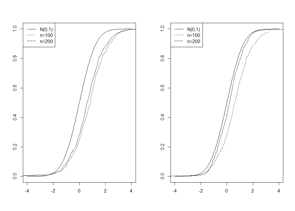
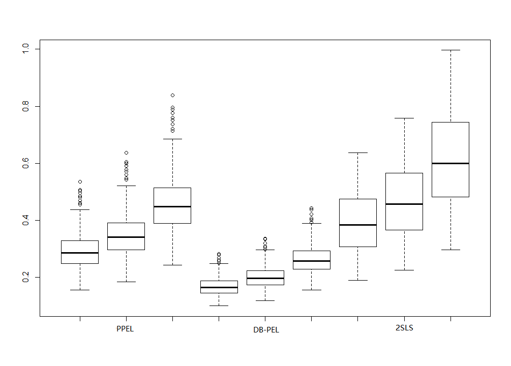
The left panel of Figure 2 plots the empirical cumulative distribution functions (ECDF) of the DB-PEL estimates. The dotted curve corresponds to the case of , the dashed curve to that of , and the solid curve is the cumulative distribution function (CDF) of for comparison. A better normal approximation can be obtained by the PPEL estimate, as shown in the right panel of Figure 2, with its tuning parameter . We also present the confidence intervals (CI) according to PPEL, DB-PEL and 2SLS, as reported in Table 3, for the 90%, 95% and 99% levels, where the CIs for DB-PEL and PPEL are predicated on the asymptotic normality from Theorems 3.1 and 5.1, respectively, and the CIs for 2SLS are based on its asymptotic normality as in standard textbooks. PPEL’s coverage probability to the nominal counterpart is the best among the three estimators, and is much better than PEL. 2SLS’s coverage probability seems too high in the high-dimensional setting, though it is acceptable in the low-dimensional case. Figure 2 shows that the width of 2SLS’s CI is much wider than that of PPEL, which is caused by efficiency loss from abandoning the potentially valid estimating equations.
| Correlation: | weak | moderate | strong | |||||||||
| Method | 90 | 95 | 99 | 90 | 95 | 99 | 90 | 95 | 99 | |||
| Panel A: low-dimensional setting | ||||||||||||
| (100, 50, 6) | PPEL | 0.894 | 0.940 | 0.988 | 0.890 | 0.940 | 0.986 | 0.888 | 0.942 | 0.986 | ||
| DB-PEL | 0.736 | 0.830 | 0.926 | 0.726 | 0.794 | 0.916 | 0.744 | 0.818 | 0.902 | |||
| 2SLS | 0.912 | 0.964 | 0.994 | 0.912 | 0.964 | 0.994 | 0.912 | 0.964 | 0.994 | |||
| (200, 100, 6) | PPEL | 0.902 | 0.950 | 0.994 | 0.902 | 0.948 | 0.994 | 0.902 | 0.946 | 0.994 | ||
| DB-PEL | 0.762 | 0.838 | 0.934 | 0.734 | 0.842 | 0.940 | 0.752 | 0.852 | 0.928 | |||
| 2SLS | 0.920 | 0.956 | 1.000 | 0.920 | 0.956 | 1.000 | 0.920 | 0.956 | 1.000 | |||
| Panel B: high-dimensional setting | ||||||||||||
| (100, 120, 6) | PPEL | 0.908 | 0.956 | 0.996 | 0.892 | 0.948 | 0.994 | 0.888 | 0.940 | 0.992 | ||
| DB-PEL | 0.746 | 0.832 | 0.922 | 0.784 | 0.850 | 0.926 | 0.768 | 0.836 | 0.936 | |||
| 2SLS | 0.956 | 0.982 | 1.000 | 0.956 | 0.982 | 1.000 | 0.956 | 0.982 | 1.000 | |||
| (200, 240, 6) | PPEL | 0.914 | 0.964 | 0.988 | 0.916 | 0.960 | 0.988 | 0.906 | 0.954 | 0.988 | ||
| DB-PEL | 0.754 | 0.846 | 0.966 | 0.778 | 0.854 | 0.958 | 0.776 | 0.866 | 0.966 | |||
| 2SLS | 0.966 | 0.992 | 1.000 | 0.966 | 0.992 | 1.000 | 0.966 | 0.992 | 1.000 | |||
| (100, 120, 8) | PPEL | 0.888 | 0.942 | 0.992 | 0.870 | 0.930 | 0.986 | 0.852 | 0.924 | 0.980 | ||
| DB-PEL | 0.778 | 0.836 | 0.904 | 0.738 | 0.818 | 0.920 | 0.730 | 0.806 | 0.910 | |||
| 2SLS | 0.960 | 0.988 | 1.000 | 0.960 | 0.988 | 1.000 | 0.960 | 0.988 | 1.000 | |||
| (200, 240, 12) | PPEL | 0.924 | 0.962 | 0.990 | 0.914 | 0.958 | 0.986 | 0.892 | 0.950 | 0.982 | ||
| DB-PEL | 0.794 | 0.872 | 0.954 | 0.788 | 0.864 | 0.946 | 0.764 | 0.860 | 0.938 | |||
| 2SLS | 0.972 | 0.998 | 1.000 | 0.972 | 0.998 | 1.000 | 0.972 | 0.998 | 1.000 | |||
| (100, 120, 13) | PPEL | 0.884 | 0.940 | 0.992 | 0.852 | 0.914 | 0.976 | 0.862 | 0.912 | 0.974 | ||
| DB-PEL | 0.788 | 0.862 | 0.938 | 0.744 | 0.798 | 0.904 | 0.688 | 0.768 | 0.882 | |||
| 2SLS | 0.942 | 0.986 | 0.996 | 0.942 | 0.986 | 0.996 | 0.942 | 0.986 | 0.996 | |||
| (200, 240, 17) | PPEL | 0.916 | 0.956 | 0.984 | 0.914 | 0.958 | 0.982 | 0.886 | 0.938 | 0.982 | ||
| DB-PEL | 0.792 | 0.884 | 0.968 | 0.780 | 0.866 | 0.954 | 0.798 | 0.864 | 0.952 | |||
| 2SLS | 0.974 | 0.988 | 1.000 | 0.974 | 0.988 | 1.000 | 0.974 | 0.988 | 1.000 | |||
7 Empirical application
Colonialism was widespread over the globe prior to the Second World War. While European institutions which protected private properties and checked government powers were successfully replicated in a few colonies, many others suffered expropriation of natural and human resources. In an influential study, Acemoglu et al. 2001 (AJR, henceforth) systematically explored the relationship between Europeans’ mortality rates and the modes of institutions.
We revisit AJR’s open-access dataset. AJR’s main structural equation is , where the dependent variable is logarithm GDP per capita in 1995, and the key explanatory variable of interest is average protection against expropriation risk, a continuous variable of a scale between 0 and 10. The latitude of a colony, denoted as , is an additional control variable. For substantial measurement errors in the institutional index can bias the OLS estimator, the credibility of the empirical evidence counts on IVs.
AJR compiled from historical documents a seminal variable logarithm of European settler mortality, and argued forcefully that it qualifies as a valid IV for the endogenous variable . Their empirical evidence was based on the 2SLS regression in cross-sectional data of countries. The baseline result in AJR’s Column (2) of Table 4 (p.1386) corresponds to the three estimating functions by the notations in our simulation, and the 2SLS reports with STD 0.22.
There are another 11 potential health variables and institutional variables, which serve as potential IVs. AJR were uncertain about their validity, and they experimented in their Table 7 (p.1392) and Table 8 (p.1394) the empirical results under various IV configurations. These variables, denoted as , are (i) Malaria in 1994, (ii) Yellow fever, (iii) Life expectancy, (iv) Infant mortality, (v) Mean temperature, (vi) Distance from coast, (vii) European settlements in 1990, (viii) Democracy (1st year of independence), (ix) Constraint on executive (1st year of independence), (x) Democracy in 1900, and (xi) Constraint on executive in 1900. (i)–(iv) are health variables, (v)–(vi) are geographic variables, and (vii)–(xi) are institutional variables. All these extra IVs are associated with the estimating functions Given the moderate sample size of 56 countries, a total of 12 IVs is non-trivial.
Our PPEL estimates the main equation as
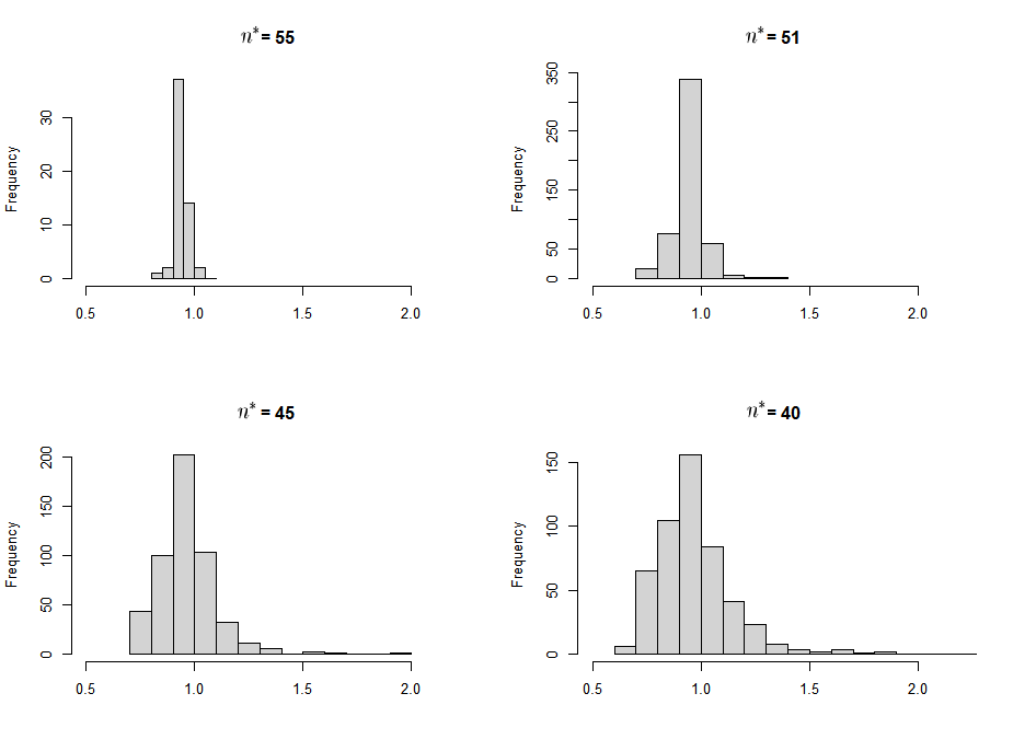
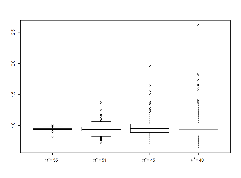
For the estimation and inference of the key parameter of interest , we compare the results of PEL, DB-PEL, PPEL and the conventional 2SLS. Its point estimation (PE), STD, and CIs are presented in Table 4. Enjoying the efficiency gain from the extra IVs, the STD of PPEL is 0.126 when we select the tuning parameter with (the boldface row), as suggested by our simulations. This STD achieves a 37% reduction relative to that of the plain 2SLS with the sole valid IV. Moreover, when we vary the constant in as 0.04, 0.06, 0.12 and 0.16, PPEL is rather robust over the wide range of tuning parameters.
| PE | STD | 95% CI | ||
| PEL | NA | 0.937 | 0.078 | (0.786, 1.090) |
| DB-PEL | NA | 0.938 | 0.078 | (0.786, 1.090) |
| 2SLS | NA | 0.945 | 0.200 | (0.553, 1.338) |
| PPEL | 0.04 | 0.942 | 0.159 | (0.631, 1.254) |
| 0.06 | 0.941 | 0.136 | (0.675, 1.207) | |
| 0.08 | 0.945 | 0.126 | (0.698, 1.193) | |
| 0.12 | 0.964 | 0.150 | (0.669, 1.259) | |
| 0.16 | 0.967 | 0.152 | (0.669, 1.266) |
Note: Our sample size is 56, after removing countries with missing variables from the original sample of 64 countries, so the 2SLS point estimate is 0.945, slightly different from AJR’s 1.00.
Our method is particularly important in unifying the IV selection in AJR’s Tables 7 and 8 into a single set of automatically selected IVs. Among the 11 potential IVs, our moment selection criterion (3.9) invalidates all institutional variables. Five IVs survive the testing: the climate variable mean temperature, the geographic variable distance from coast, and three health variables dummy of yellow fever, infant mortality and life expectancy. All the other health and institutional variables are assessed as endogenous and are unsuitable for IVs in this study. The justification for mean temperature and distance from coast is straightforward because humans were unable to interfere with these natural conditions in the era of colonialism. Furthermore, AJR argued for the validity of dummy of yellow fever, though due to concerns of lack of variation they did not employ it as the main IV (AJR’s p.1393, Paragraph 2). Our variable selection result provides supportive evidence to AJR’s heuristics.
8 Conclusion
This paper considers a general setting of an economic structural model with many potential moments, some of which may be invalid. These invalid moments must be disciplined in order to estimate the structural parameter consistently. We propose a PEL approach to estimate the parameter of interest while coping with the invalid moments. We show that the PEL estimator is normally distributed asymptotically, and invalid moments can be consistently detected thanks to the oracle property. To overcome the difficulty of estimating the bias in the limiting distribution of the PEL estimator, we further devise the PPEL approach for statistical inference of a low-dimensional object of interest, which is useful for hypothesis testing and confidence region construction. Simulation exercises are carried out to demonstrate excellent finite sample performance of our methods. We revisit an empirical application concerning economic development and shed new insight about its candidate instruments.
Supplementary materials
The supplementary materials consist of three parts. Part A provides the proofs and technical details about the methods developed in the present article. Part B reports additional simulation results concerning the liner IV model in the main text and an additional dynamic panel data model, respectively. Part C checks the robustness of PEL in the empirical application.
References
- (1)
- Acemoglu et al. (2001) Acemoglu, D., Johnson, S. and Robinson, J. A. (2001), ‘The colonial origins of comparative development: An empirical investigation’, The American Economic Review 91(5), 1369–1401.
- Ackerberg et al. (2007) Ackerberg, D., Benkard, C. L., Berry, S. and Pakes, A. (2007), ‘Econometric tools for analyzing market outcomes’, Handbook of Econometrics 6, 4171–4276.
- Altonji and Segal (1996) Altonji, J. G. and Segal, L. (1996), ‘Small-sample bias in gmm estimation of covariance structures’, Journal of Business & Economic Statistics 14(3), 353–366.
- Altonji et al. (2013) Altonji, J. G., Smith, A. A. J. and Vidangos, I. (2013), ‘Modeling earnings dynamics’, Econometrica 81(4), 1395–1454.
- Anatolyev and Gospodinov (2011) Anatolyev, S. and Gospodinov, N. (2011), Methods for Estimation and Inference in Modern Econometrics, CRC Press.
- Andrews and Cheng (2012) Andrews, D. and Cheng, X. (2012), ‘Estimation and inference with weak, semi-strong, and strong identification’, Econometrica 80(5), 2153–2211.
- Andrews and Lu (2001) Andrews, D. and Lu, B. (2001), ‘Consistent model and moment selection procedures for gmm estimation with application to dynamic panel data models’, Journal of Econometrics 101(1), 123–164.
- Andrews and Mikusheva (2020) Andrews, I. and Mikusheva, A. (2020), ‘Optimal decision rules for weak gmm’, arXiv preprint arXiv:2007.04050 .
- Andrews et al. (2019) Andrews, I., Stock, J. H. and Sun, L. (2019), ‘Weak instruments in instrumental variables regression: Theory and practice’, Annual Review of Economics 11, 727–753.
- Angrist (1990) Angrist, J. D. (1990), ‘Lifetime earnings and the vietnam era draft lottery: Evidence from social security administrative records’, The American Economic Review 80(3), 313–336.
- Angrist and Keueger (1991) Angrist, J. D. and Keueger, A. B. (1991), ‘Does compulsory school attendance affect schooling and earnings?’, The Quarterly Journal of Economics 106(4), 979–1014.
- Angrist and Krueger (1992) Angrist, J. D. and Krueger, A. B. (1992), ‘The effect of age at school entry on educational attainment: An application of instrumental variables with moments from two samples’, Journal of the American Statistical Association 87(418), 328–336.
- Bekker (1994) Bekker, P. A. (1994), ‘Alternative approximations to the distributions of instrumental variable estimators’, Econometrica 62(3), 657–681.
- Belloni et al. (2012) Belloni, A., Chen, D., Chernozhukov, V. and Hansen, C. (2012), ‘Sparse models and methods for optimal instruments with an application to eminent domain’, Econometrica 80(6), 2369–2429.
- Belloni et al. (2018) Belloni, A., Chernozhukov, V., Chetverikov, D., Hansen, C. and Kato, K. (2018), ‘High-dimensional econometrics and regularized gmm’, arXiv preprint arXiv:1806.01888 .
- Belloni et al. (2014) Belloni, A., Chernozhukov, V. and Hansen, C. (2014), ‘Inference on treatment effects after selection among high-dimensional controls’, The Review of Economic Studies 81(2), 608–650.
- Bertsekas (1997) Bertsekas, D. P. (1997), ‘Nonlinear programming’, Journal of the Operational Research Society 48(3), 334–334.
- Bickel et al. (2009) Bickel, P. J., Ritov, Y. and Tsybakov, A. B. (2009), ‘Simultaneous analysis of lasso and dantzig selector’, The Annals of Statistics 37(4), 1705–1732.
- Blundell et al. (1993) Blundell, R., Pashardes, P. and Weber, G. (1993), ‘What do we learn about consumer demand patterns from micro data?’, The American Economic Review 83(3), 570–597.
- Bühlmann (2013) Bühlmann, P. (2013), ‘Statistical significance in high-dimensional linear models’, Bernoulli 19(4), 1212–1242.
- Candes and Tao (2007) Candes, E. and Tao, T. (2007), ‘The dantzig selector: Statistical estimation when p is much larger than n’, The Annals of Statistics 35(6), 2313–2351.
- Caner and Fan (2015) Caner, M. and Fan, Q. (2015), ‘Hybrid generalized empirical likelihood estimators: Instrument selection with adaptive lasso’, Journal of Econometrics 187(1), 256–274.
- Caner et al. (2018) Caner, M., Han, X. and Lee, Y. (2018), ‘Adaptive elastic net gmm estimation with many invalid moment conditions: Simultaneous model and moment selection’, Journal of Business & Economic Statistics 36(1), 24–46.
- Caner and Kock (2018) Caner, M. and Kock, A. B. (2018), ‘High dimensional linear gmm’, arXiv preprint arXiv:1811.08779 .
- Chang et al. (2015) Chang, J., Chen, S. X. and Chen, X. (2015), ‘High dimensional generalized empirical likelihood for moment restrictions with dependent data’, Journal of Econometrics 185(1), 283–304.
- Chang et al. (2021) Chang, J., Chen, S. X., Tang, C. Y. and Wu, T. T. (2021), ‘High-dimensional empirical likelihood inference’, Biometrika 108(1), 127–147.
- Chang et al. (2018) Chang, J., Tang, C. Y. and Wu, T. T. (2018), ‘A new scope of penalized empirical likelihood with high-dimensional estimating equations’, The Annals of Statistics 46(6B), 3185–3216.
- Chang et al. (2013) Chang, J., Tang, C. Y. and Wu, Y. (2013), ‘Marginal empirical likelihood and sure independence feature screening’, The Annals of Statistics 41(4), 2123–2148.
- Chao et al. (2011) Chao, J. C., Swanson, N. R., Hausman, J. A., Newey, W. K. and Woutersen, T. (2011), ‘Asymptotic distribution of jive in a heteroskedastic iv regression with many instruments’, Econometric Theory 28(1), 42–86.
- Chen and Chen (2008) Chen, J. and Chen, Z. (2008), ‘Extended bayesian information criteria for model selection with large model spaces’, Biometrika 95(3), 759–771.
- Cheng and Liao (2015) Cheng, X. and Liao, Z. (2015), ‘Select the valid and relevant moments: An information-based lasso for gmm with many moments’, Journal of Econometrics 186(2), 443–464.
- DiTraglia (2016) DiTraglia, F. J. (2016), ‘Using invalid instruments on purpose: Focused moment selection and averaging for gmm’, Journal of Econometrics 195(2), 187–208.
- Eaton et al. (2011) Eaton, J., Kortum, S. and Kramarz, F. (2011), ‘An anatomy of international trade: Evidence from french firms’, Econometrica 79(5), 1453–1498.
- Fan and Li (2001) Fan, J. and Li, R. (2001), ‘Variable selection via nonconcave penalized likelihood and its oracle properties’, Journal of the American Statistical Association 96(456), 1348–1360.
- Fan and Liao (2014) Fan, J. and Liao, Y. (2014), ‘Endogeneity in high dimensions’, The Annals of Statistics 42(3), 872–917.
- Gold et al. (2020) Gold, D., Lederer, J. and Tao, J. (2020), ‘Inference for high-dimensional instrumental variables regression’, Journal of Econometrics 217(1), 79–111.
- Hall et al. (2007) Hall, A. R., Inoue, A., Jana, K. and Shin, C. (2007), ‘Information in generalized method of moments estimation and entropy-based moment selection’, Journal of Econometrics 138(2), 488–512.
- Han et al. (2005) Han, C., Orea, L. and Schmidt, P. (2005), ‘Estimation of a panel data model with parametric temporal variation in individual effects’, Journal of Econometrics 126(2), 241–267.
- Han and Phillips (2006) Han, C. and Phillips, P. (2006), ‘Gmm with many moment conditions’, Econometrica 74(1), 147–192.
- Hansen and Kozbur (2014) Hansen, C. and Kozbur, D. (2014), ‘Instrumental variables estimation with many weak instruments using regularized jive’, Journal of Econometrics 182(2), 290–308.
- Hansen (1982) Hansen, L. (1982), ‘Large sample properties of generalized method of moments estimators’, Econometrica 50(4), 1029–1054.
- Hansen et al. (1996) Hansen, L., Heaton, J. and Yaron, A. (1996), ‘Finite-sample properties of some alternative gmm estimators’, Journal of Business & Economic Statistics 14(3), 262–280.
- Hjort et al. (2009) Hjort, N. L., McKeague, I. W. and Van Keilegom, I. (2009), ‘Extending the scope of empirical likelihood’, The Annals of Statistics 37(3), 1079–1111.
- Hong et al. (2003) Hong, H., Preston, B. and Shum, M. (2003), ‘Generalized empirical likelihood-based model selection criteria for moment condition models’, Econometric Theory 19(6), 923–943.
- Jing et al. (2003) Jing, B.-Y., Shao, Q.-M. and Wang, Q. (2003), ‘Self-normalized cramér-type large deviations for independent random variables’, The Annals of Probability 31(4), 2167–2215.
- Kitamura (2001) Kitamura, Y. (2001), ‘Asymptotic optimality of empirical likelihood for testing moment restrictions’, Econometrica 69(6), 1661–1672.
- Kleibergen (2005) Kleibergen, F. (2005), ‘Testing parameters in gmm without assuming that they are identified’, Econometrica 73(4), 1103–1123.
- Koenker and Machado (1999) Koenker, R. and Machado, J. (1999), ‘Gmm inference when the number of moment conditions is large’, Journal of Econometrics 93(2), 327–344.
- Kolesár et al. (2015) Kolesár, M., Chetty, R., Friedman, J., Glaeser, E. and Imbens, G. W. (2015), ‘Identification and inference with many invalid instruments’, Journal of Business & Economic Statistics 33(4), 474–484.
- Kumbhakar (1990) Kumbhakar, S. C. (1990), ‘Production frontiers, panel data, and time-varying technical inefficiency’, Journal of Econometrics 46(1-2), 201–211.
- Leng and Tang (2012) Leng, C. and Tang, C. Y. (2012), ‘Penalized empirical likelihood and growing dimensional general estimating equations’, Biometrika 99(3), 703–716.
- Liao (2013) Liao, Z. (2013), ‘Adaptive gmm shrinkage estimation with consistent moment selection’, Econometric Theory 29(5), 857–904.
- Lv and Fan (2009) Lv, J. and Fan, Y. (2009), ‘A unified approach to model selection and sparse recovery using regularized least squares’, The Annals of Statistics 37(6A), 3498–3528.
- Matsushita and Otsu (2013) Matsushita, Y. and Otsu, T. (2013), ‘Second-order refinement of empirical likelihood for testing overidentifying restrictions’, Econometric Theory 29(2), 324–353.
- Mavroeidis (2005) Mavroeidis, S. (2005), ‘Identification issues in forward-looking models estimated by gmm, with an application to the phillips curve’, Journal of Money, Credit and Banking 37(3), 421–448.
- Murray (2006) Murray, M. P. (2006), ‘Avoiding invalid instruments and coping with weak instruments’, Journal of Economic Perspectives 20(4), 111–132.
- Newey and Smith (2003) Newey, W. K. and Smith, R. J. (2003), ‘Higher order properties of gmm and generalized empirical likelihood estimators’, Econometrica 72(1), 219–255.
- Newey and Windmeijer (2009) Newey, W. K. and Windmeijer, F. (2009), ‘Generalized method of moments with many weak moment conditions’, Econometrica 77(3), 687–719.
- Neykov et al. (2018) Neykov, M., Ning, Y., Liu, J. S. and Liu, H. (2018), ‘A unified theory of confidence regions and testing for high-dimensional estimating equations’, Statistical Science 33(3), 427–443.
- Ning and Liu (2017) Ning, Y. and Liu, H. (2017), ‘A general theory of hypothesis tests and confidence regions for sparse high dimensional models’, The Annals of Statistics 45(1), 158–195.
- Otsu (2006) Otsu, T. (2006), ‘Generalized empirical likelihood inference for nonlinear and time series models under weak identification’, Econometric Theory 22(3), 513–527.
- Otsu (2007) Otsu, T. (2007), ‘Penalized empirical likelihood estimation of semiparametric models’, Journal of Multivariate Analysis 98(10), 1923–1954.
- Otsu (2010) Otsu, T. (2010), ‘On bahadur efficiency of empirical likelihood’, Journal of Econometrics 157(2), 248–256.
- Owen (1988) Owen, A. B. (1988), ‘Empirical likelihood ratio confidence intervals for a single functional’, Biometrika 75(2), 237–249.
- Owen (1990) Owen, A. B. (1990), ‘Empirical likelihood ratio confidence regions’, The Annals of Statistics 18(1), 90–120.
- Petrov (1995) Petrov, V. V. (1995), Limit Theorems of Probability Theory: Sequences of Independent Random Variables, Clarendon Press, Oxford.
- Qin and Lawless (1994) Qin, J. and Lawless, J. (1994), ‘Empirical likelihood and general estimating equations’, The Annals of Statistics 22(1), 300–325.
- Roodman (2009) Roodman, D. (2009), ‘A note on the theme of too many instruments’, Oxford Bulletin of Economics and Statistics 71(1), 135–158.
- Rudin (1976) Rudin, W. (1976), Principles of Mathematical Analysis, McGraw-Hill, New York.
- Shi (2016a) Shi, Z. (2016a), ‘Econometric estimation with high-dimensional moment equalities’, Journal of Econometrics 195(1), 104–119.
- Shi (2016b) Shi, Z. (2016b), ‘Estimation of sparse structural parameters with many endogenous variables’, Econometric Reviews 35(8-10), 1582–1608.
- Stock and Wright (2000) Stock, J. H. and Wright, J. H. (2000), ‘Gmm with weak identification’, Econometrica 68(5), 1055–1096.
- Stock et al. (2014) Stock, J. H., Wright, J. H. and Yogo, M. (2014), ‘A survey of weak instruments and weak identification in generalized method of moments’, Journal of Business & Economic Statistics 20(4), 518–529.
- Stock and Yogo (2005) Stock, J. H. and Yogo, M. (2005), ‘Testing for weak instruments in linear iv regression’, Identification and Inference for Econometric Models: Essays in Honor of Thomas Rothenberg pp. 109–120.
- Tang and Leng (2010) Tang, C. Y. and Leng, C. (2010), ‘Penalized high-dimensional empirical likelihood’, Biometrika 97(4), 905–920.
- Windmeijer et al. (2019) Windmeijer, F., Farbmacher, H., Davies, N. and Smith, G. D. (2019), ‘On the use of the lasso for instrumental variables estimation with some invalid instruments’, Journal of the American Statistical Association 114(527), 1339–1350.
- Zhang (2010) Zhang, C.-H. (2010), ‘Nearly unbiased variable selection under minimax concave penalty’, The Annals of Statistics 38(2), 894–942.
- Zhang and Huang (2008) Zhang, C.-H. and Huang, J. (2008), ‘The sparsity and bias of the lasso selection in high-dimensional linear regression’, The Annals of Statistics 36(4), 1567–1594.
- Zou (2006) Zou, H. (2006), ‘The adaptive Lasso and its oracle properties’, Journal of the American Statistical Association 101(476), 1418–1429.
Supplement to “Culling the Herd of Moments with Penalized Empirical Likelihood”
Jinyuan Chang, Zhentao Shi, and Jia Zhang
This supplement consists of three parts. Part A provides the proofs and technical details about the method developed in the present article. Part B reports additional simulation results concerning the liner IV model in the main text and an additional dynamic panel data model, respectively. Part C checks the robustness of PEL in the empirical application.
We use “” to denote a generic positive finite constant that may be different in different uses.
A Theoretical details and technical proofs
A.1 Proposition A.1
Let and define Proposition A.1 gives the asymptotic normality of the standard EL estimator .
Proposition A.1.
Assume that: (i) There exists a universal constant such that
| (A.1) |
for any . (ii) There exist universal constants , and such that
| (A.2) | ||||
| (A.3) |
with . (iii) Each element of is twice continuously differentiable with respect to for any , and
| (A.4) |
where is specified in (A.2). (iv) There exists a universal constant such that
| (A.5) |
where (v) and . Then
as for any with .
Remark A.1.
To understand the relative magnitude of , and , consider the special case with and fixed , under which satisfies the condition. This is consistent with the literature of GMM involving a diverging number of moments under a fixed (Koenker and Machado 1999); when diverges, is sufficient for the asymptotic normality in Proposition A.1.
Remark A.2.
Strong identification of the parameter of interest is assumed in (A.1). It is possible to generalize on the right-hand side of (A.1) to for some universal constant at the cost of much complicated expressions for the admissible range of and . (A.2) restricts the population moments uniformly over the parameter space. (A.3) and (A.5) bound away from zero and infinity the eigenvalues of and , respectively. The first and second derivatives of the estimating functions are further regularized by (A.4).
Remark A.3.
If there are some envelope functions such that for any , and for any integer , where and are two universal positive constants independent of , Petrov 1995’s Theorem 2.8 implies provided ; the other two requirements in (A.4) can be satisfied in the same manner. The stochastic order in (A.4) can be replaced by for some diverging . Our theoretical results still hold in this broader situation at the expense of more complicated restrictions among , and .
Proof. Define for any and . Then and its associated Lagrange multiplier satisfy the score equation , i.e.
By the Taylor expansion, we have
for some , which implies
By the implicit function theorem [Theorem 9.28 of Rudin 1976], for all in a -neighborhood of , there is a such that and is continuously differentiable in . By the concavity of with respect to (w.r.t) , . It follows from the envelope theorem that
Therefore, we have
| (A.6) |
Define and let . As shown in the proof of Proposition 1 of Chang et al. 2018, we have which implies . As , we have . We will first show that for any satisfying , there exists a universal constant independent of such that as for any satisfying . Thus . Notice that we can select an arbitrary slowly diverging , to ensure , following a standard result from probability theory. To do this, we will use the technique developed for the proof of Theorem 1 in Chang et al. 2013. For any satisfying , let . Define and where is a constant to be determined later, and is an -dimensional vector with the -th component being and other components being . Without loss of generality, we assume . (A.2) and the Markov inequality yield that , which implies . Then with probability approaching one (w.p.a.1). Write . By the definition of , it holds w.p.a.1 that
for some and . Therefore, it holds that
From (A.2) and the Markov inequality, there exists a universal positive constant independent of such that as . Thus, with , we have
From (A.1), we know that with specified in (A.1). For sufficiently small independent of , we have for some , which implies that Since for some , it holds that . Therefore, we have .
Under (A.2) and (A.3), Proposition 1 of Chang et al. 2018 implies that . It follows from the Taylor expansion that for some between and . Similar to Lemma 3 of Chang et al. 2018, we know holds uniformly over . If and , (A.5) implies that is uniformly bounded away from zero w.p.a.1. Recall . Then , which implies . Repeating the proof of Lemma 3 of Chang et al. 2018, we can improve the convergence rate of . More specifically, holds uniformly over . Identical to the proof of Proposition 1 of Chang et al. 2018, we have . Under (A.3) and (A.4), similar to Lemmas 1–3 of Chang et al. 2018, we have the following two results:
and
holds uniformly over . Therefore, by (A.6), for any with finite -norm, we have
| (A.7) |
Recall , and holds uniformly over . Thus, (A.7) implies
| (A.8) |
For any with unit -norm, let . Write and . Notice that . Then,
Then, it follows from (A.3) and (A.5) that . From (A.8), the Central Limit Theorem implies that
provided that and .
A.2 Proof of Proposition 2.2
Define and . Let and be the associated ’s such that and . Due to , and , we have . Due to , and , letting , we have . Since , then . Hence, . Notice that . Then . Since (2.2) has a unique solution, we have .
A.3 Proof of Proposition 3.1
As we have defined in Section 3, with for any , where is a prescribed constant. Define for any and . For any index set and , we write . For any and , we define
| (A.9) | ||||
Write . Recall that , with , and for some fixed . Then
The proof of Proposition 3.1 requires the following lemmas. The proof of Lemma A.1 is similar to that of Lemma 1 in Chang et al. 2018 and we omit it here. Lemma A.2 presents general properties of the Lagrange multiplier when is in a small neighborhood of , whose proof is given in Section A.7.1. If we just focus on the properties of , Lemma A.3 states a refined version of Lemma A.2 with proof given in Section A.7.2.
Lemma A.2.
Let be a sequence in and be a convex function for defined as (3.2). For some , assume that all the eigenvalues of are uniformly bounded away form zero and infinity w.p.a.1. Let for some , and . For some non-random sequence such that as , if and , then w.p.a.1 there is a sparse global maximizer for satisfying the following three results: (i) , (ii) , and (iii) for any with , where .
Lemma A.3.
Let be a convex function for defined as (3.2). Assume that all the eigenvalues of are uniformly bounded away from zero and infinity w.p.a.1 for some , and . If and , then w.p.a.1 there is a sparse global maximizer for satisfying .
Now we begin to prove Proposition 3.1. Recall and . Then , where . Let and write . It holds that
| (A.10) |
where for some open interval containing zero. We will first prove that
| (A.11) |
Based on (A.11), we have . Let and . As we have shown in the proof of Lemma A.3 that w.p.a.1, it then follows from Lemma A.3 that w.p.a.1. Pick and , which can be guaranteed by . Define and let . It follows from the last requirement of Condition 3 that , which implies that . By the Taylor expansion, it holds w.p.a.1 that
| (A.12) |
for some , where the last inequality is implied by Condition 4 and Lemma A.1. As we have shown in the proof of Lemma A.3 that , then . It follows from (A.12) that . Hence, w.p.a.1. Since w.p.a.1, by the concavity of and the convexity of , we have w.p.a.1. Then we can obtain (A.11) from (A.12).
Recall that . Then . Notice that with , and . We then have which implies that . We need to show w.p.a.1, which indicates that is a local minimizer of . Our proof includes three parts: (i) to show that for any satisfying and any satisfying , there exists a universal constant independent of such that as . Due to , we can select an arbitrary slowly diverging satisfying . Thus, we have ; (ii) letting and , to show that for any satisfying and satisfying and , there exists a universal constant independent of such that as . Recall . Due to , we know w.p.a.1. Since we can select an arbitrary slowly diverging satisfying , it holds that ; (iii) to show that w.p.a.1.
Proof of Part (i). The proof is similar to that for Part (i) of Proposition A.1. For any satisfying , let and . Select , where is a sufficiently small constant, and is an -dimensional vector with the -th component being and other components being . Then w.p.a.1. Without loss of generality, we assume that . Write . Notice that . By the Taylor expansion, it holds w.p.a.1 that . Thus,
Using the same arguments stated in the proof of Proposition A.1, we have as . We complete the proof of Part (i).
Proof of Part (ii). The proof is also similar to that for Part (i) of Proposition A.1. For any with satisfying and , let and . Without loss of generality, we assume . Select , where is a sufficiently small constant, and is similarly defined as that in the proof of Part (i). Then w.p.a.1. By the Taylor expansion, it holds w.p.a.1 that . Thus,
By the Taylor expansion and Condition 3, . Recall and . Then
| (A.13) |
when is sufficiently large. Using the same arguments stated in the proof of Proposition A.1, we have as . We complete the proof of Part (ii).
Proof of Part (iii). If , we define and will show w.p.a.1. This contradicts the definition of . Then we have w.p.a.1. Write and . Recall for any and for any . As shown in Part (ii) that , due to and (3.5), (A.10) and (A.11) imply that
| (A.14) | ||||
Notice that . We pick and . Recall with for any . Define
for some . Select satisfying and . Since w.p.a.1, it holds that , which indicates that w.p.a.1. Write .
Recall for any . Notice that for some constant . Then w.p.a.1 by letting . Notice that . By the Taylor expansion, it holds w.p.a.1 that
for some . Thus, . For any , choose satisfying and . Then, . Using the same arguments given above, we can obtain , which implies that . Since we can select an arbitrary slow , we have following a standard result from probability theory. Then Lemmas A.1 and A.2 imply that . Recall . Write and . Notice that and . Then
| (A.15) | ||||
It follows from the Taylor expansion that
| (A.16) |
where is on the jointing line between and . We need to show w.p.a.1.
To do this, we first use Lemma A.2 to bound . Given some , we define
It holds that
| (A.17) | ||||
As we have shown that , then . For the term in (A.17), we have
Notice that . Then . Recall for any . Due to , it holds that for any . Hence, . Analogously, we also have . For the term , notice that for any , we have and for some . Since , it holds that w.p.a.1, which implies that w.p.a.1. Therefore, we have . Together with Lemma A.2, we have , which implies for specified in (A.16).
Recall and . We have . For , since , we have
| (A.18) |
As we have shown , it then holds . On the other hand, in (A.16) satisfies for some . Due to , we can obtain w.p.a.1, which implies that w.p.a.1. We complete the proof of Part (iii).
A.4 Proof of Theorem 3.1
Select as the sparse local minimizer given in Proposition 3.1. Recall that the estimate is the Lagrange multiplier associated with , where for any and . Write . Recall , and . Then can be decomposed into three disjoint sets . Write . Notice that and . Then and . For any , we have . To prove Theorem 3.1, we also need the following two lemmas. The proof of Lemma A.4 is similar to that of Lemma 3 in Chang et al. 2018 and we omit it here. The proof of Lemma A.5 is given in Section A.7.3.
Lemma A.4.
Lemma A.5.
Now we begin to prove Theorem 3.1. Define
| (A.19) |
By the definition of , we have , that is,
where with for , for and , and for . It follows from the Taylor expansion that
| (A.20) |
for some . Hence, . By the definition of , we have . Notice that
Due to , then . On the other hand, Lemma A.5 implies that . Thus, . Together with (A.20), we have
| (A.21) | ||||
where . Recall that . Proposition 3.1 and (3.5) imply that w.p.a.1. To construct the asymptotic normality, we need the following lemma. The proof of Lemma A.6 is similar to that of Lemma 2 in Chang et al. 2018 and we omit it here.
Lemma A.6.
Assume the conditions of Proposition 3.1 hold. Then , and holds uniformly over .
Recall
| (A.22) |
For any with unit -norm, let . Following the same arguments stated in the proof of Proposition A.1, we have . Lemma A.2 indicates that w.p.a.1 for some . As we have shown in the proof of Proposition 3.1, it holds that
Together with Lemmas A.1, A.4, and A.6, (A.21) implies that
Notice that and . By the Taylor expansion, we have w.p.a.1, where is on the line joining and . Recall that with and . Notice that , and . For any and , we know that does not involve , which implies that . Therefore, it holds that w.p.a.1, which leads to
| (A.25) | ||||
Next, we will specify the convergence rate of . Since , it follows from (A.4) that . On the other hand, it holds that , where is on the line joining and . Similar to Lemma A.4, Condition 5 implies that . Hence, by similar arguments of Lemma A.4, we have . Recall with defined in (A.22). Recall . It follows from (A.25) that
Lemma 4 of Chang et al. 2018 yields . Then as .
Notice that . In the sequel, we will specify the limiting distribution of . Recall and . We write , and with following blocks
where is a matrix, and is an matrix. Recall and . Then . By (A.22), we have . For any with unit -norm, let . Then . Hence, , where is the first components of . We complete the proof of Theorem 3.1.
A.5 Proof of Theorem 4.1
Recall and with in the current setting. Define and . Then . Notice that with for any , where is a prescribed constant. Recall for any and . In this section, we redefine
| (A.26) |
for any and , where is defined as (A.9) in Section A.3. In comparison to defined in Section A.3 for a low-dimensional , the newly defined here for a high-dimensional has an extra term which is caused by the penalty imposed on . Write and . Recall . Then and . Similar to that in Section A.3, we define for some fixed . Consider
| (A.27) |
Analogously to Proposition 3.1, here Proposition A.2 shows that such defined is a sparse local minimizer for the nonconvex optimization (4.1).
Proposition A.2.
Let for defined as (3.2), and be convex with bounded second derivative around . Let with , , and . For defined as (A.27), assume that there exists a constant such that . Under Conditions 1′, 2–4 and (4.4), if , , , and , then w.p.a.1 such defined provides a local minimizer for the nonconvex optimization (4.1) such that (i) , (ii) as , (iii) , and (iv) as .
Since involved here for high-dimensional is identical to that used in Section A.3 for low-dimensional , Lemmas A.2 and A.3 still hold in the the current setting. With the newly defined for high-dimensional , Lemma A.1 also holds in the current setting. The proof of Proposition A.2 is almost identical to that of Proposition 3.1. Using the same arguments as those in the proof of Proposition 3.1, we obtain . Recall that and . Then . Notice that with , and . We then have which implies . We need to show w.p.a.1, which indicates that is a local minimizer of .
We now follow a slightly different line of proof: (i) to show that for any satisfying and any satisfying , there exists a universal constant independent of such that as . Due to , we can select an arbitrary slowly diverging satisfying . Thus, we have ; (ii) to show that for any satisfying and satisfying and , there exists a universal constant independent of such that as . Since w.p.a.1 and we can select an arbitrary slowly diverging satisfying , it holds that ; (iii) to show that w.p.a.1.
The proof of Part (i) is similar to that of Proposition 2 in Chang et al. 2018. For any with satisfying , take and . Let and . Select , where is a constant to be determined later, and is an -dimensional vector with the -th component being and other components being . Then w.p.a.1. For the newly defined in (A.26), applying the identical arguments for proof of Part (i) in Section A.3, we still have
Condition 1′ implies that with specified in Condition 1′, and for sufficiently large , which implies for sufficiently large . Using the same arguments stated in the proof of Proposition A.1, we have as . The proof of Part (ii) and Part (iii) are almost identical to that of Proposition 3.1, except some small adjustments. The first difference is for deriving the lower bound of appeared in the proof of Part (ii). Notice that . Hence, identical to (A.13), we still have when is sufficiently large. The second difference is (A.14). In the current setting, it should be
where and . The third difference is that the index set in (A.15) should be replaced by due to the newly defined in the current setting. Then (A.16) changes to
The last difference appears in the upper bound of . Since and , we now have
where the upper bound has an extra factor in comparison to (A.18). Due to , it then holds . Also notice that for some . Then is required for Proposition A.2 rather than required in Proposition 3.1.
Select as the sparse local minimizer given in Proposition A.2. Recall , and . Notice that and . Then and . For any , we have . Under the conditions of Proposition A.2, the results of Lemmas A.4 and A.5 hold with the newly defined , , , , , and . The proof of Theorem 4.1 is almost identical to that of Theorem 3.1 stated in Section A.4. We only point out the difference here. The first difference is the definition of . In comparison to given in (A.19) for the low-dimensional , we define
in current high-dimensional setting. Following the same arguments stated in Section A.4, (A.21) still holds with . It follows from Proposition A.2 that w.p.a.1. Notice that Lemma A.6 still holds in the current setting. Identical to the arguments below (A.21), it holds that as . Notice that . Recall and . We write , and with following blocks
where is a matrix, and is an matrix. Recall and . Then . By the same arguments of Theorem 3.1, we complete the proof of Theorem 4.1.
A.6 Proof of Theorem 5.1
Now we begin to prove Theorem 5.1. Let . By the same arguments in the proof of Lemma A.7 for bounding there, we have . Identical to (A.6), it holds that
where
for some . Write . Similar to Lemma A.6, , and holds uniformly over . Let . For any , let , and it holds that
Expanding near , we obtain
| (A.28) | ||||
where is on the line joining and . By Condition 3, we have . Moreover, by the proof of Theorem 1 in Chang et al. 2021, if and , we have . Together with (A.28), it holds that
Let with . If and , then by similar arguments in the proof of Lemma 4 of Chang et al. 2018, we have
We complete the proof.
A.7 Proofs of auxiliary lemmas
A.7.1 Proof of Lemma A.2
To simplify the notation, we write and as and , respectively. Due to the convexity of , we know that is a concave function w.r.t . We only need to show there exists a sparse local maximizer satisfying the three results. By the definition of and , we have which implies w.p.a.1. Notice that . Given , we select satisfying and . Let where . It follows from that holds uniformly over , which implies that . Thus, . By the Taylor expansion, we have
| (A.29) |
where and . Recall . By the convexity of , we have for any . Notice that is uniformly bounded away from zero w.p.a.1, and . Thus, (A.29) leads to
Due to , it holds that . Recall . Then and . Write . We have w.p.a.1 that
| (A.30) |
where with for and for . It follows from (A.30) that with
which indicates that . Hence, w.p.a.1 we have for any with . To complete the proof, we need to show that is a local maximizer of w.p.a.1. Our proof includes two steps.
Step 1. Define for some sufficiently small , where with for some constant . For defined before, we will show in this step that w.p.a.1. Due to and , we know w.p.a.1. Restricted on , by the concavity of w.r.t , it suffices to show that w.p.a.1 for any it holds that
| (A.31) |
Due to and , then is an interior point of the set . Restricted on , we know is concave w.r.t . Notice that . Therefore, (A.31) holds for any . Recall . For any , we have and
where the term is uniform over . Such conclusion can be obtained by the same arguments for deriving the convergence rate of stated above. By the definition of and , we know . Then for any . Hence, we have w.p.a.1 that
which implies that there exists some such that
Hence, (A.31) holds for any . Then we have w.p.a.1.
Step 2. Define . We will prove in this step that is the maximizer of over . Notice that . For any , denote by the projection of onto for defined in Step 1. Then it holds that
where is on the jointing line between and . It follows from the Taylor expansion that
where the term holds uniformly over . Since , then w.p.a.1. Thus,
Hence, is a local maximizer of w.p.a.1. We complete the proof of Lemma A.2.
A.7.2 Proof of Lemma A.3
To simplify the notation, we write and as and , respectively. Recall with and . Due to , by the moderate deviation of self-normalized sums (Jing et al. 2003), it holds that provided that . Since , we know which implies w.p.a.1. Pick satisfying and which can be guaranteed by . Recall with for some . Then w.p.a.1. Let and . Due to holds uniformly over , we have . Write . Similar to (A.29), we have
for some . Due to , we have . Then . Using the same arguments to prove is a local maximizer of w.p.a.1 in the proof of Lemma A.2, we can also show such defined is a local maximizer of w.p.a.1. Notice that is a concave function w.r.t . We complete the proof.
A.7.3 Proof of Lemma A.5
Recall for any and , and . Then and its associated Lagrange multiplier satisfy the score equation , that is,
where with for , for and , and for and . Recall . Restricted on , for any and with for any , define , where with for and otherwise. Then and satisfy . By the implicit function theorem [Theorem 9.28 of Rudin 1976], for all in a -neighbourhood of , there is a such that , and is continuously differentiable in .
By Condition 6, we know the event holds w.p.a.1. Restricted on , let . Define for some . Since for any and is continuously differentiable in , we can select sufficiently small such that for any and . For any , let satisfy and . We will show that for any w.p.a.1. Restricted on , for any , we have
where is on the line joining and , is on the line joining and , and the terms and hold uniformly over . Notice that . Therefore, it holds w.p.a.1 that
On the other hand, since , and for any , then it holds that
for any , where , and for any . By the concavity of with respect to , we know for any w.p.a.1. Therefore, is continuously differentiable at and w.p.a.1. We complete the proof.
A.7.4 Proof of Lemma A.7
By the proof of Theorem 1 in Chang et al. 2021, we have provided that and . Next, we will specify the convergence rate of . Define for any and . Let . Pick and . Let where . Conditions 3 and 7 imply that , which implies . Under Conditions 4 and 7, if and , Lemma 4 of Chang et al. 2021 implies that the eigenvalues of are uniformly bounded away from zero and infinity w.p.a.1. By the Taylor expansion, we have
for some . Since , then which implies w.p.a.1. Due to w.p.a.1 and the concavity of , w.p.a.1 and . For specified above, let and then . Similar to Lemma 4 of Chang et al. 2021, under Conditions 4 and 7, if and , we have the eigenvalues of are uniformly bounded away from zero and infinity w.p.a.1. Applying the Taylor expansion again, it holds that
for some , which implies that . Given any , let . Repeating above arguments again, we have . Notice that we can select an arbitrary slow . Then .
Notice that , where is on the jointing line between and . Recall and let . Then . Write and denote by the columns of that are indexed in . Recall is a -dimensional vector with its -th component being and all other components being . Then . Hence, the eigenvalues of are uniformly bounded away from zero. Analogously to Lemma A.4, we have holds uniformly over . Then, if and , it holds that w.p.a.1, which implies . We complete the proof.
B Additional numerical results
Due to limitations of space, in the main text we report the simulation results of the linear IV model only. In this section, we display additional results for the linear IV model, and also experiment with a nonlinear model.
B.1 Linear IV model
Although economists are primarily interested in the effect of the endogenous variable, the exogenous variables in control other sources of heterogeneity. To render a full picture of the performance of the estimation, we report the simulation results of and —the coefficients for the exogenous variables and —from the linear IV model in the main text.
| Correlation: | weak | moderate | strong | |
| Panel A: low-dimensional setting | ||||
| (100, 50, 6) | PEL | 0.172 | 0.176 | 0.167 |
| 2SLS | 0.219 | 0.219 | 0.219 | |
| (200, 100, 6) | PEL | 0.114 | 0.115 | 0.115 |
| 2SLS | 0.152 | 0.152 | 0.152 | |
| Panel B: high-dimensional setting | ||||
| (100, 120, 6) | PEL | 0.175 | 0.183 | 0.177 |
| 2SLS | 0.245 | 0.245 | 0.245 | |
| (200, 240, 6) | PEL | 0.124 | 0.125 | 0.122 |
| 2SLS | 0.199 | 0.199 | 0.199 | |
| (100, 120, 8) | PEL | 0.207 | 0.211 | 0.207 |
| 2SLS | 0.300 | 0.300 | 0.300 | |
| (200, 240, 12) | PEL | 0.114 | 0.113 | 0.113 |
| 2SLS | 0.188 | 0.188 | 0.188 | |
| (100, 120, 13) | PEL | 0.220 | 0.239 | 0.213 |
| 2SLS | 0.293 | 0.293 | 0.293 | |
| (200, 240, 17) | PEL | 0.130 | 0.133 | 0.126 |
| 2SLS | 0.199 | 0.199 | 0.199 | |
Table S1 displays the RMSE of PEL and 2SLS for . Here,
where denotes the number of repetitions and denotes the estimate of in the -th repetition. The RMSE of 2SLS is significantly larger than that of PEL, showing that the advantages of PEL extend to the estimation for the coefficients of the exogenous variables.
| Correlation: | weak | moderate | strong | |||||||||
| Method | 90 | 95 | 99 | 90 | 95 | 99 | 90 | 95 | 99 | |||
| Panel A: low-dimensional setting | ||||||||||||
| (100, 50, 6) | 0.892 | 0.948 | 0.992 | 0.888 | 0.948 | 0.992 | 0.890 | 0.950 | 0.992 | |||
| 0.874 | 0.930 | 0.990 | 0.868 | 0.926 | 0.990 | 0.870 | 0.928 | 0.990 | ||||
| (200, 100, 6) | 0.898 | 0.940 | 0.988 | 0.896 | 0.936 | 0.988 | 0.894 | 0.938 | 0.988 | |||
| 0.880 | 0.938 | 0.984 | 0.880 | 0.936 | 0.986 | 0.882 | 0.936 | 0.986 | ||||
| Panel B: high-dimensional setting | ||||||||||||
| (100, 120, 6) | 0.878 | 0.940 | 0.984 | 0.870 | 0.942 | 0.980 | 0.874 | 0.932 | 0.980 | |||
| 0.892 | 0.930 | 0.978 | 0.884 | 0.926 | 0.972 | 0.886 | 0.926 | 0.970 | ||||
| (200, 240, 6) | 0.896 | 0.936 | 0.976 | 0.894 | 0.936 | 0.976 | 0.892 | 0.938 | 0.976 | |||
| 0.878 | 0.934 | 0.986 | 0.872 | 0.934 | 0.986 | 0.868 | 0.936 | 0.986 | ||||
| (100, 120, 8) | 0.870 | 0.924 | 0.976 | 0.866 | 0.926 | 0.974 | 0.864 | 0.928 | 0.974 | |||
| 0.854 | 0.928 | 0.976 | 0.850 | 0.924 | 0.960 | 0.834 | 0.916 | 0.964 | ||||
| (200, 240, 12) | 0.886 | 0.954 | 0.994 | 0.884 | 0.952 | 0.994 | 0.874 | 0.942 | 0.994 | |||
| 0.892 | 0.940 | 0.980 | 0.892 | 0.938 | 0.980 | 0.886 | 0.938 | 0.980 | ||||
| (100, 120, 13) | 0.872 | 0.934 | 0.990 | 0.862 | 0.918 | 0.988 | 0.860 | 0.918 | 0.984 | |||
| 0.864 | 0.930 | 0.982 | 0.842 | 0.916 | 0.974 | 0.848 | 0.916 | 0.976 | ||||
| (200, 240, 17) | 0.898 | 0.944 | 0.988 | 0.896 | 0.944 | 0.990 | 0.892 | 0.942 | 0.988 | |||
| 0.908 | 0.948 | 0.976 | 0.902 | 0.948 | 0.974 | 0.900 | 0.940 | 0.974 | ||||
The coverage probabilities for the CIs of and are summarized in Table S2. It reveals the strength of PPEL for the inference of these coefficients. Moreover, Figure S1 characterizes the shape of the confidence regions for the cases and with moderate correlation between and .

B.2 Dynamic panel data model
Consider a simplified panel data model with time-varying individual heterogeneity (Han et al. 2005):
where the zero mean error term may potentially correlate with the individual-specific fixed effect , and the nonlinear specification , , is originated from Kumbhakar 1990. Here we use , instead of , to represent the panel’s time dimension in order to be consistent with the notations throughout the paper.
Notice that the fixed effect can be canceled out by
where and The above equation implies many moment conditions when varies.
The parameter of interest lies in , which determines the speed of decay of the individual-specific shock , whereas is an intercept. In the simulation exercises, the true parameter is set as . Let and we specify and , , and i.i.d across time. All data across individuals are independent. The number of known valid moments is fixed to be , and then the number of validity-unknown moments is . After periods, there occurs a structural break in the mean where the intercept shifts from to and these corresponding moments become invalid at . The number of invalid moments is and when and , respectively, and for small, moderate, and large shifts, respectively. The choice of the tuning parameters stays the same as that in the linear model.
Tables S3–S5 are the counterparts of Tables 1–3 in the high-dimensional setting. In Table S3, correct moment selection improves with the sample size, and FN quickly goes to zero as increases. As shown in Table S5, PEL offers reasonable estimation of the parameter while bias correction is difficult in this nonlinear model as well. In Table S5, PPEL again exhibits more accurate coverage probability than DB-PEL. Our proposed estimation and inference procedures are effective in terms of moment selection, parameter estimation and coverage probability in this nonlinear panel data model with many moments.
| 0.2 | 0.3 | 0.4 | |||||||
| Method | FP | FN | FP | FN | FP | FN | |||
| (100, 120, 6) | PEL | 0.0874 | 0.1600 | 0.0980 | 0.0060 | 0.0984 | 0.0000 | ||
| DB-PEL | 0.0872 | 0.1600 | 0.0980 | 0.0060 | 0.0983 | 0.0000 | |||
| (200, 240, 6) | PEL | 0.0168 | 0.0607 | 0.0237 | 0.0000 | 0.0166 | 0.0000 | ||
| DB-PEL | 0.0168 | 0.0607 | 0.0237 | 0.0000 | 0.0166 | 0.0000 | |||
| (100, 120, 8) | PEL | 0.0986 | 0.1218 | 0.0937 | 0.0080 | 0.0914 | 0.0000 | ||
| DB-PEL | 0.0985 | 0.1220 | 0.0936 | 0.0080 | 0.0913 | 0.0000 | |||
| (200, 240, 12) | PEL | 0.0305 | 0.0253 | 0.0303 | 0.0000 | 0.0167 | 0.0000 | ||
| DB-PEL | 0.0305 | 0.0253 | 0.0303 | 0.0000 | 0.0167 | 0.0000 | |||
| (100, 120, 13) | PEL | 0.0988 | 0.1292 | 0.1009 | 0.0055 | 0.0926 | 0.0000 | ||
| DB-PEL | 0.0987 | 0.1292 | 0.1007 | 0.0055 | 0.0924 | 0.0000 | |||
| (200, 240, 17) | PEL | 0.0394 | 0.0178 | 0.0305 | 0.0000 | 0.0395 | 0.0000 | ||
| DB-PEL | 0.0394 | 0.0178 | 0.0305 | 0.0000 | 0.0395 | 0.0000 | |||
| 0.2 | 0.3 | 0.4 | ||||||||||
| Method | RMSE | BIAS | STD | RMSE | BIAS | STD | RMSE | BIAS | STD | |||
| (100, 120, 6) | PEL | 0.053 | 0.000 | 0.053 | 0.053 | 0.003 | 0.053 | 0.053 | 0.003 | 0.053 | ||
| DB-PEL | 0.062 | 0.003 | 0.062 | 0.058 | 0.004 | 0.058 | 0.058 | 0.004 | 0.058 | |||
| (200, 240, 6) | PEL | 0.038 | 0.005 | 0.038 | 0.039 | 0.005 | 0.038 | 0.039 | 0.005 | 0.038 | ||
| DB-PEL | 0.042 | 0.004 | 0.041 | 0.043 | 0.004 | 0.042 | 0.042 | 0.005 | 0.041 | |||
| (100, 120, 8) | PEL | 0.053 | 0.002 | 0.053 | 0.053 | 0.003 | 0.053 | 0.053 | 0.003 | 0.053 | ||
| DB-PEL | 0.058 | 0.004 | 0.058 | 0.058 | 0.003 | 0.058 | 0.058 | 0.004 | 0.058 | |||
| (200, 240, 12) | PEL | 0.039 | 0.005 | 0.038 | 0.039 | 0.005 | 0.038 | 0.039 | 0.005 | 0.038 | ||
| DB-PEL | 0.042 | 0.004 | 0.041 | 0.041 | 0.005 | 0.041 | 0.042 | 0.004 | 0.042 | |||
| (100, 120, 13) | PEL | 0.053 | 0.001 | 0.053 | 0.053 | 0.003 | 0.053 | 0.053 | 0.003 | 0.053 | ||
| DB-PEL | 0.056 | 0.002 | 0.056 | 0.056 | 0.004 | 0.056 | 0.056 | 0.004 | 0.056 | |||
| (200, 240, 17) | PEL | 0.038 | 0.005 | 0.038 | 0.039 | 0.005 | 0.038 | 0.039 | 0.005 | 0.038 | ||
| DB-PEL | 0.042 | 0.004 | 0.042 | 0.041 | 0.004 | 0.041 | 0.042 | 0.004 | 0.041 | |||
| 0.2 | 0.3 | 0.4 | ||||||||||
| Method | 90 | 95 | 99 | 90 | 95 | 99 | 90 | 95 | 99 | |||
| (100, 120, 6) | PPEL | 0.894 | 0.954 | 0.994 | 0.882 | 0.934 | 0.986 | 0.914 | 0.952 | 0.990 | ||
| DB-PEL | 0.836 | 0.900 | 0.974 | 0.862 | 0.932 | 0.988 | 0.844 | 0.922 | 0.986 | |||
| (200, 240, 6) | PPEL | 0.888 | 0.930 | 0.980 | 0.896 | 0.952 | 0.990 | 0.882 | 0.926 | 0.974 | ||
| DB-PEL | 0.846 | 0.904 | 0.980 | 0.834 | 0.906 | 0.978 | 0.828 | 0.904 | 0.984 | |||
| (100, 120, 8) | PPEL | 0.886 | 0.926 | 0.986 | 0.902 | 0.954 | 0.980 | 0.908 | 0.960 | 0.984 | ||
| DB-PEL | 0.868 | 0.924 | 0.978 | 0.848 | 0.938 | 0.974 | 0.834 | 0.920 | 0.982 | |||
| (200, 240, 12) | PPEL | 0.894 | 0.948 | 0.986 | 0.896 | 0.948 | 0.990 | 0.898 | 0.952 | 0.978 | ||
| DB-PEL | 0.846 | 0.906 | 0.980 | 0.848 | 0.914 | 0.978 | 0.834 | 0.910 | 0.974 | |||
| (100, 120, 13) | PPEL | 0.906 | 0.960 | 0.984 | 0.896 | 0.946 | 0.978 | 0.876 | 0.938 | 0.984 | ||
| DB-PEL | 0.878 | 0.932 | 0.982 | 0.870 | 0.920 | 0.984 | 0.864 | 0.928 | 0.980 | |||
| (200, 240, 17) | PPEL | 0.926 | 0.952 | 0.990 | 0.894 | 0.950 | 0.992 | 0.912 | 0.960 | 0.990 | ||
| DB-PEL | 0.844 | 0.896 | 0.982 | 0.844 | 0.918 | 0.980 | 0.838 | 0.908 | 0.978 | |||
C Robustness of empirical application
To check the stability of PEL estimator in the real data analysis, we draw bootstrap samples from the original data and apply the proposed method to these sub-samples. Specifically, to witness the effect of sample sizes, we draw from the original sample with no replacement bootstrap observations and , which correspond to the sub-samples of size , , and , respectively. Given a sub-sample, the proposed PEL method is used to estimate the coefficient . We repeat the bootstrap exercise for 500 times. The results are summarized in Figure S2. The point estimate from the true sample is 0.937, and the bootstrap point estimates are well centered around it. Regarding the histograms, despite a thin right tail when , the dispersion quickly concentrates as increases. The normal distribution appears to be an effective approximation when is above 50.