跳到论文正文
W Papers独立论文阅读器 arXiv:2108.03223 论文正文 计算阅读时间 · 0%
引用这篇论文根据当前论文元数据生成,正式投稿前建议核对。


License: arXiv.org perpetual non-exclusive license
arXiv:2108.03223v1 [quant-ph] 06 Aug 2021

Mitigating off-resonant error in the cross-resonance gate

Moein Malekakhlagh Email: Electronic address: moein.malekakhlagh@ibm.com Affiliation: IBM Quantum, IBM Thomas J. Watson Research Center, 1101 Kitchawan Rd, Yorktown Heights, NY 10598    Easwar Magesan Email: Electronic address: emagesa@us.ibm.com Affiliation: IBM Quantum, IBM Thomas J. Watson Research Center, 1101 Kitchawan Rd, Yorktown Heights, NY 10598
August 11, 2026
Abstract

Off-resonant error for a driven quantum system refers to interactions due to the input drives having non-zero spectral overlap with unwanted system transitions. For the cross-resonance gate, this includes leakage as well as off-diagonal computational interactions that lead to bit-flip error on the control qubit. In this work, we quantify off-resonant error, with more focus on the less studied off-diagonal control interactions, for a direct CNOT gate implementation. Our results are based on numerical simulation of the dynamics, while we demonstrate the connection to time-dependent Schrieffer-Wolff and Magnus perturbation theories. We present two methods for suppressing such error terms. First, pulse parameters need to be optimized so that off-resonant transition frequencies coincide with the local minima due to the pulse spectrum sidebands. Second, we show the advantage of a YY-DRAG pulse on the control qubit in mitigating off-resonant error. Depending on qubit-qubit detuning, the proposed methods can improve the average off-resonant error from approximately 10−310^{-3} closer to the 10−410^{-4} level for a direct CNOT calibration.

I Introduction

Cross-resonance (CR) is a microwave-activated two-qubit gate performed by driving one of the qubits (control) at the frequency of the other (target) Paraoanu_Microwave_2006; Rigetti_Fully_2010. In this architecture, superconducting qubits Nakamura_Coherent_1999; Wallraff_Strong_2004; Koch_Charge_2007; Clarke_Superconducting_2008, typically fixed-frequency transmons Koch_Charge_2007, connect via a mediating bus resonator, resulting in a static qubit-qubit exchange interaction. The CR protocol induces various two-qubit interactions Sheldon_Procedure_2016; Magesan_Effective_2020; Kirchhoff_Optimized_2018; Tripathi_Operation_2019; Malekakhlagh_First-Principles_2020; Sundaresan_Reducing_2020; Heya_Cross_2021, with Z​XZX as the dominant rate, through which a CNOT gate can be calibrated. Simplicity in implementation, resilience to charge and flux noise, and scalability has made CR architecture the leading workhorse for current IBM quantum processors Cross_Validating_2019; Sundaresan_Reducing_2020; Jurcevic_Demonstration_2021.

Improving CR gate fidelity necessitates both an accurate understanding of the effective interactions as well as precise microwave control. In particular, a multi-level analysis of the dynamics Sheldon_Procedure_2016; Magesan_Effective_2020; Kirchhoff_Optimized_2018; Tripathi_Operation_2019; Malekakhlagh_First-Principles_2020; Sundaresan_Reducing_2020 is required for CR gate implementation with weakly anharmonic transmon qubits Koch_Charge_2007. Higher qubit states can lead to both renormalization of interactions in the computational subspace Magesan_Effective_2020; Malekakhlagh_First-Principles_2020; Sundaresan_Reducing_2020 as well as out-of-computational leakage Wood_Quantification_2018; Tripathi_Operation_2019. Generally, to optimize the coherent fidelity, we need to maximize the desired Z​XZX rate and minimize unwanted computational and leakage interactions.

There are two main CNOT calibration schemes based on CR architecture. First, an echo sequence consisting of two CR pulses with flipped amplitude accompanied with single-qubit rotations Sheldon_Procedure_2016; Malekakhlagh_First-Principles_2020; Sundaresan_Reducing_2020; Jurcevic_Demonstration_2021. The echo removes certain unwanted rates such as the Z​IZI, Z​ZZZ and I​XIX, while induces higher order I​YIY and I​ZIZ error terms Malekakhlagh_First-Principles_2020; Sundaresan_Reducing_2020. Reference Jurcevic_Demonstration_2021 demonstrated a 280280 ns echoed CR gate with an average fidelity of 99.40%99.40\%. Second, a direct CNOT calibration with a single CR pulse Tripathi_Operation_2019; Kandala_Demonstration_2020; Jurcevic_Demonstration_2021. To this aim, we want no operation on the target qubit when the control is in state |0c⟩\ket{0_{c}}, hence canceling I​X+Z​XIX+ZX via a separate drive on the target, and a π\pi rotation on the target when the control is in state |1c⟩\ket{1_{c}}. Therefore, the I​XIX rate is not an error term anymore, and CR gate speed is determined by twice the Z​XZX (I​XIX) rate, resulting in a faster gate. Equipped with multiple-path interference couplers Mundada_Suppression_2019 to suppress the static Z​ZZZ rate, and using virtual frame change McKay_Efficient_2017 to cancel out Stark shifts in software, Ref. Kandala_Demonstration_2020 demonstrated a 180180 ns gate with 99.77%99.77\% average gate fidelity.

Schrieffer-Wolff Perturbation Theory (SWPT) Schrieffer_Relation_1966; Boissonneault_Dispersive_2009; Bravyi_Schrieffer_2011; Gambetta_Analytic_2011; Malekakhlagh_Lifetime_2020; Petrescu_Lifetime_2020; Magesan_Effective_2020; Malekakhlagh_First-Principles_2020; Petrescu_Accurate_2021 is a central method in our analytical understanding of effective interactions. SWPT provides effective models by averaging high-frequency off-resonant processes systematically. Through a series of perturbative frame transformations, the interactions are partitioned into resonant (effective) and off-resonant categories. The effective interactions come from processes that connect states with equal frequency in the rotating-frame of the drive, while off-resonant interactions have a net non-zero transition frequency. In contrast to rotating-wave approximation (RWA), which simply discards off-resonant terms, SWPT takes them into account by solving for and storing the relevant frame transformations. Hence, contributions that are not resonant at a specific order may lead to resonant interactions via non-trivial higher order mixings. The drive scheme, and the corresponding energy diagram, determines the choice of the effective frame. For CR, where the drive is resonant with the target qubit, the effective SWPT frame is block-diagonal (BD) with respect to the control Magesan_Effective_2020. Under the BD approximation, analytical estimates for CR gate parameters have been derived in Refs. Magesan_Effective_2020; Malekakhlagh_First-Principles_2020 for constant-amplitude continuous wave (CW) drive.

In this paper, we study off-resonant error due to interactions that originate from the CR drive frequency being detuned from states of the control qubit. The corresponding dominant unwanted transitions are |0c⟩↔|1c⟩\ket{0_{c}}\leftrightarrow\ket{1_{c}}, |0c⟩↔|2c⟩\ket{0_{c}}\leftrightarrow\ket{2_{c}} and |1c⟩↔|2c⟩\ket{1_{c}}\leftrightarrow\ket{2_{c}} (see Fig. 1). Although off-resonant error is present for a CW drive, there is an intricate interplay with the pulse shape and in particular the pulse ramps. To model this, we employ numerical simulations based on Magnus expansion Magnus_Exponential_1954; Blanes_Magnus_2009; Blanes_Pedagogical_2010; Hairer_Geometric_2006. Furthermore, we extend our SWPT formalism for CR in Refs. Magesan_Effective_2020; Malekakhlagh_First-Principles_2020 to the time-dependent case and make a connection to the Magnus method. In particular, the main role of time-independent and dependent perturbations are to account for how strong the drive amplitude and how fast (non-adiabatic) the pulse ramps are compared to the system transition frequencies, respectively. These two effects are independent in general, however, in the context of gate calibration, they become related based on a fixed rotation angle imposed by the intended gate.

Generally, to mitigate off-resonant error, CR drive should have minimal spectral content at the unwanted transition frequencies. Qubit-qubit detuning and anharmonicity determine the relative configuration of off-resonant transitions in the rotating-frame of the drive Tripathi_Operation_2019; Malekakhlagh_First-Principles_2020, where the error due to one or sometimes multiple transitions can be noticeable. We take the standard square Gaussian pulse, i.e. flat top with Gaussian ramps, and demonstrate further improvement. The most immediate refinement comes from optimization of the pulse rise time known as Gaussian shaping Chow_Optimized_2010; Gambetta_Analytic_2011. It should be set so that the transition for the most dominant error type overlaps with one of the local minima of the pulse sidebands. Moreover, we show additional improvement by a YY-DRAG Motzoi_Simple_2009; Chow_Optimized_2010; Gambetta_Analytic_2011; Schutjens_Single-Qubit_2013 pulse on the control qubit. We argue that, in essence, DRAG acts as an effective filter that can be tuned to notch the error due to specific off-resonant transitions.

The remainder of this paper is organized as follows. In Sec. II, we introduce our model for a direct CNOT gate implementation Tripathi_Operation_2019; Kandala_Demonstration_2020. In Sec. III, we discuss the theory behind off-resonant error, by relating time-dependent SWPT to the Magnus method, which extends our earlier results in Refs. Magesan_Effective_2020; Malekakhlagh_First-Principles_2020. Furthermore, using numerical simulation based on Magnus, we quantify the dependence of off-resonant error on pulse parameters. In Sec. IV, we demonstrate the advantage of YY-DRAG pulse on the control qubit in suppressing off-resonant error.

There are five appendices. In Appendix A, we discuss the derivation of a generalized time-dependent SWPT to account for the underlying pulse shapes. Using the SWPT formalism, Appendix B derives effective time-dependent Hamiltonian rates generalizing Refs. Magesan_Effective_2020; Tripathi_Operation_2019; Malekakhlagh_First-Principles_2020. Appendices C and D provide the effective time evolution operator and the corresponding leading order non-BD contributions, respectively. In Appendix E, we derive leading order estimates for dominant off-resonant error types, and corresponding DRAG conditions for their suppression.

Refer to caption
Figure 1: (a) CR gate schematic with separate drives on each qubit. The drive amplitudes Ωj​(t)≡Ωj​x​(t)+i​Ωj​y​(t)\Omega_{j}(t)\equiv\Omega_{jx}(t)+i\Omega_{jy}(t), j=c,tj=c,t are complex-valued to allow for more involved control schemes like DRAG Motzoi_Simple_2009; Chow_Optimized_2010; Gambetta_Analytic_2011; Schutjens_Single-Qubit_2013. The drive frequency is set to the target qubit frequency. (b) Energy diagram in the rotating frame of the drive under RWA (see Sec. II). The control-target detuning is denoted by Δc​t≡ωc−ωt\Delta_{ct}\equiv\omega_{c}-\omega_{t}, and control and target anharmonicities by αc\alpha_{c} and αt\alpha_{t}, respectively.

II Direct CNOT

We consider two coupled transmon qubits Koch_Charge_2007 with individual drive on each qubit. The transmon Hamiltonian can be approximated in terms of multi-level Kerr oscillators as

ℋ^q≡∑j=c,t[ωj​b^j†​b^j+αj2​b^j†​b^j†​b^j​b^j],\displaystyle\hat{\mathcal{H}}_{q}\equiv\sum\limits_{j=c,t}\left[\omega_{j}\hat{b}_{j}^{{\dagger}}\hat{b}_{j}+\frac{\alpha_{j}}{2}\hat{b}_{j}^{{\dagger}}\hat{b}_{j}^{{\dagger}}\hat{b}_{j}\hat{b}_{j}\right]\;, (1)

with ωc,t\omega_{c,t} and αc,t\alpha_{c,t} denoting the corresponding frequency and anharmonicity for the control and the target qubits, respectively. The transmon-transmon exchange interaction takes the approximate form

ℋ^J≡J⁡(b^c†​b^t+b^c​b^t†),\displaystyle\hat{\mathcal{H}}_{J}\equiv J\left(\hat{b}_{c}^{{\dagger}}\hat{b}_{t}+\hat{b}_{c}\hat{b}_{t}^{{\dagger}}\right)\;, (2)

where JJ is the effective exchange rate as a result of either direct capacitive coupling or mediated coupling through a common bus resonator Magesan_Effective_2020; Malekakhlagh_First-Principles_2020. Furthermore, we consider separate drives on each qubit as

ℋ^d​(t)≡12​[Ωc∗​(t)​b^c​ei​ωd​t+Ωc​(t)​b^c†​e−i​ωd​t]+12​[Ωt∗​(t)​b^t​ei​ωd​t+Ωt​(t)​b^t†​e−i​ωd​t],\displaystyle\begin{split}\hat{\mathcal{H}}_{d}(t)&\equiv\frac{1}{2}\left[\Omega_{c}^{*}(t)\hat{b}_{c}e^{i\omega_{d}t}+\Omega_{c}(t)\hat{b}_{c}^{{\dagger}}e^{-i\omega_{d}t}\right]\\ &+\frac{1}{2}\left[\Omega_{t}^{*}(t)\hat{b}_{t}e^{i\omega_{d}t}+\Omega_{t}(t)\hat{b}_{t}^{{\dagger}}e^{-i\omega_{d}t}\right],\end{split} (3)

with frequency ωd\omega_{d}, same as target qubit frequency, and time-dependent complex-valued pulse amplitudes Ωc​(t)≡Ωc​x​(t)+i​Ωc​y​(t)\Omega_{c}(t)\equiv\Omega_{cx}(t)+i\Omega_{cy}(t) and Ωt​(t)≡Ωt​x​(t)+i​Ωt​y​(t)\Omega_{t}(t)\equiv\Omega_{tx}(t)+i\Omega_{ty}(t) (see Fig. 1). The phase of the microwave drive determines the axis, in the XX–YY plane of the target qubit, to which the drive couples. We set the main CR drive to couple to the XX quadrature of the target, while the YY axis can be used for DRAG following the same conventions as single-qubit gates Motzoi_Simple_2009; Gambetta_Analytic_2011; Schutjens_Single-Qubit_2013. In our numerical and perturbative analysis, the system Hamiltonian is the static part ℋ^s≡ℋ^q+ℋ^J\hat{\mathcal{H}}_{s}\equiv\hat{\mathcal{H}}_{q}+\hat{\mathcal{H}}_{J}, accounting for the dressing due to J, and the interaction-frame Hamiltonian is defined as ℋ^I​(t)≡exp⁡(i​ℋ^s​t)​ℋ^d​(t)​exp⁡(−i​ℋ^s​t)\hat{\mathcal{H}}_{I}(t)\equiv\exp(i\hat{\mathcal{H}}_{s}t)\hat{\mathcal{H}}_{d}(t)\exp(-i\hat{\mathcal{H}}_{s}t).

In Eqs. (1)–(3), we have adopted a Kerr model for the qubits, and applied RWA in both drive and exchange interactions. This RWA neglects terms that oscillate at approximately twice the target qubit frequency, of the order of 10 GHz, and does not change the physics of the CR gate qualitatively. Our goal here is to work with the simplest model to focus mainly on more dominant error that comes from off-resonant transitions of the control qubit, with transition frequencies of the order of 100 MHz, and study the dependence on pulse parameters. A more precise model for the CR gate was discussed in our earlier work Malekakhlagh_First-Principles_2020, accounting also for eigenstate renormalization due to counter-rotating terms in the Josephson nonlinearity.

Tuning a direct CNOT gate Kandala_Demonstration_2020 requires identity operation on the target qubit when the control is in state |0c⟩\ket{0_{c}} so that

ωi​x​(t)+ωz​x​(t)=0,\displaystyle\omega_{ix}(t)+\omega_{zx}(t)=0\;, (4)

and a π\pi rotation around the XX axis when the control is in state |1c⟩\ket{1_{c}} as

∫0τpd​t​[ωi​x​(t)−ωz​x​(t)]=π,\displaystyle\int_{0}^{\tau_{p}}dt\,[\omega_{ix}(t)-\omega_{zx}(t)]=\pi\;, (5)

where ωσj​σk​(t)≡(1/2)​Tr​{ℋ^CR,eff​(t)​(σ^j⊗σ^k)}\omega_{\sigma_{j}\sigma_{k}}(t)\equiv(1/2)\text{Tr}\{\hat{\mathcal{H}}_{\text{CR,eff}}(t)\left(\hat{\sigma}_{j}\otimes\hat{\sigma}_{k}\right)\}, j,k∈{i,x,y,z}j,k\in\{i,x,y,z\}, are effective Hamiltonian rates defined over the dressed two-qubit pauli operators. For notation simplicity, we use I^≡σ^i\hat{I}\equiv\hat{\sigma}_{i}, X^≡σ^x\hat{X}\equiv\hat{\sigma}_{x}, Y^≡σ^y\hat{Y}\equiv\hat{\sigma}_{y}, Z^≡σ^z\hat{Z}\equiv\hat{\sigma}_{z} and drop explicit tensor product for two-qubit Pauli operators, e.g. Z^​X^≡σ^z⊗σ^x\hat{Z}\hat{X}\equiv\hat{\sigma}_{z}\otimes\hat{\sigma}_{x}. Time-dependent SWPT provides reasonable ballparks for the effective gate parameters (see Appendices A and B). In particular, based on Eq. (4), the main cancellation tone on the target is found as

Ωt​x​(t)=JΔc​t​Ωc​x​(t)−αc​J2​Δc​t3​(2​Δc​t+αc)​Ωc​x3​(t)+O⁡(Ωc​x5),\displaystyle\Omega_{tx}(t)=\frac{J}{\Delta_{ct}}\Omega_{cx}(t)-\frac{\alpha_{c}J}{2\Delta_{ct}^{3}(2\Delta_{ct}+\alpha_{c})}\Omega_{cx}^{3}(t)+O\left(\Omega_{cx}^{5}\right), (6)

while for CNOT calibration [Eq. (5)] the main pulse should satisfy approximately

2​αc​JΔc​t​(Δc​t+αc)​Ωc​x​[τp−s1​(τr)]−(9​Δc​t3+15​Δc​t2​αc+11​Δc​t​αc2+3​αc3)​αc2​JΔc​t3​(Δc​t+αc)3​(2​Δc​t+αc)​(2​Δc​t+3​αc)×Ωc​x3​[τp−s3​(τr)]+O⁡(Ωc​x5)=π.\displaystyle\begin{split}&\frac{2\alpha_{c}J}{\Delta_{ct}(\Delta_{ct}+\alpha_{c})}\Omega_{cx}[\tau_{p}-s_{1}(\tau_{r})]\\ &-\frac{(9\Delta_{ct}^{3}+15\Delta_{ct}^{2}\alpha_{c}+11\Delta_{ct}\alpha_{c}^{2}+3\alpha_{c}^{3})\alpha_{c}^{2}J}{\Delta_{ct}^{3}(\Delta_{ct}+\alpha_{c})^{3}(2\Delta_{ct}+\alpha_{c})(2\Delta_{ct}+3\alpha_{c})}\\ &\times\Omega_{cx}^{3}[\tau_{p}-s_{3}(\tau_{r})]+O\left(\Omega_{cx}^{5}\right)=\pi\;.\end{split} (7)

Equations (6)–(7) provide a useful initial guess for drive parameters and facilitate more involved numerical optimization. We also find non-adiabatic corrections to the effective gate parameters in terms of the pulse derivatives, e.g. terms proportional to J​Ω˙c​x2​(t)​Ωc​x​(t)J\dot{\Omega}_{cx}^{2}(t)\Omega_{cx}(t) in ωi​x​(t)\omega_{ix}(t) and ωz​x​(t)\omega_{zx}(t) (see Appendix B). Here, τp\tau_{p} and τr\tau_{r} denote the gate and the rise times, respectively. Moreover, sn​(τr)s_{n}(\tau_{r}) characterizes the reduced area under the curve during the ramps, compared to a square pulse, for the nnth power of the pulse shape. In our simulations, we use the common square Gaussian pulse Jurcevic_Demonstration_2021; Kandala_Demonstration_2020.

Coherent error, compared to an ideal CNOT, can be traced back to the two aforementioned categories of interactions. Resonant (effective) error arises from faulty resonant rotations, terms like I​X​(I​Y)IX\ (IY) and Z​X​(Z​Y)ZX\ (ZY), or static and dynamic frequency shifts of the qubits, like I​ZIZ, Z​IZI and Z​ZZZ rates. Static Z​ZZZ can in principle be substantially suppressed via tunable VanDerPloeg_Controllable_2007; Chen_Qubit_2014; McKay_High-Contrast_2015; Stehlik_Tunable_2021, opposite-anharmonicity Ku_Suppression_2020; Zhao_High_2020 and multiple-path Yan_Tunable_2018; Mundada_Suppression_2019; Sung_Realization_2020; Collodo_Implementation_2020; Xu_High-Fidelity_2020; Kandala_Demonstration_2020 couplers, and also via auxiliary AC Stark tones (siZZle) on the qubits Wei_Quantum_2021; Mitchell_Hardware_2021. Furthermore, Stark shifts can be removed effectively through virtual frame change in software McKay_Efficient_2017; Kandala_Demonstration_2020. In the following, we explore the physics of off-resonant error.
Refer to caption
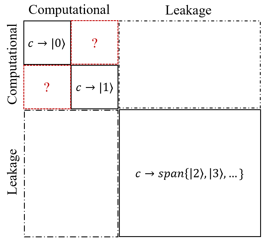
Figure 2: Schematic of the BD subspace shown in solid black, subspace corresponding to coupling between computational and leakage in dashed-dotted black, and non-BD computational subspace in red dotted lines. We are particularly interested in characterizing the error due to non-BD interactions of the form σ^x⊗σ^k\hat{\sigma}_{x}\otimes\hat{\sigma}_{k} or σ^y⊗σ^k\hat{\sigma}_{y}\otimes\hat{\sigma}_{k} for k=i,x,y,zk=i,x,y,z.
Probability Type Time-domain Frequency-domain
|0c⟩→|1c⟩\ket{0_{c}}\rightarrow\ket{1_{c}} (1) non-BD ≈14​|∫0τpd​t′​Ωc​(t′)​ei​Δc​t​t′|2\approx\frac{1}{4}\Big|\int_{0}^{\tau_{p}}dt^{\prime}\Omega_{c}(t^{\prime})e^{i\Delta_{ct}t^{\prime}}\Big|^{2} ≈14​|∫−∞+∞d​ω′2​π​Ω~c​(ω′)ω′+Δc​t​[ei⁡(ω′+Δc​t)​τp−1]|2\approx\frac{1}{4}\Big|\int\limits_{-\infty}^{+\infty}\frac{d\omega^{\prime}}{2\pi}\frac{\tilde{\Omega}_{c}(\omega^{\prime})}{\omega^{\prime}+\Delta_{ct}}\left[e^{i(\omega^{\prime}+\Delta_{ct})\tau_{p}}-1\right]\Big|^{2}
|0c⟩→|2c⟩\ket{0_{c}}\rightarrow\ket{2_{c}} (2) Leakage ≈132|∫0τpd​t′​∫0t′d​t′′​Ωc​(t′)​Ωc​(t′′)\approx\frac{1}{32}\Big|\int_{0}^{\tau_{p}}dt^{\prime}\int_{0}^{t^{\prime}}dt^{\prime\prime}\Omega_{c}(t^{\prime})\Omega_{c}(t^{\prime\prime}) [ei⁡(Δc​t+αc)​t′ei​Δc​t​t′′−ei​Δc​t​t′ei⁡(Δc​t+αc)​t′′]|2\left[e^{i(\Delta_{ct}+\alpha_{c})t^{\prime}}e^{i\Delta_{ct}t^{\prime\prime}}-e^{i\Delta_{ct}t^{\prime}}e^{i(\Delta_{ct}+\alpha_{c})t^{\prime\prime}}\right]\Big|^{2} ≈132|∫−∞+∞∫−∞+∞d​ω′2​π​d​ω′′2​π​αc​Ω~c​(ω′)​Ω~c​(ω′′)(ω′′+Δc​t+αc)​(ω′′+Δc​t)\approx\frac{1}{32}\Big|\int\limits_{-\infty}^{+\infty}\int\limits_{-\infty}^{+\infty}\frac{d\omega^{\prime}}{2\pi}\frac{d\omega^{\prime\prime}}{2\pi}\frac{\alpha_{c}\tilde{\Omega}_{c}(\omega^{\prime})\tilde{\Omega}_{c}(\omega^{\prime\prime})}{(\omega^{\prime\prime}+\Delta_{ct}+\alpha_{c})(\omega^{\prime\prime}+\Delta_{ct})} [ei⁡(ω′+ω′′+2​Δc​t+αc)​τp−1]ω′+ω′′+2​Δc​t+αc|2\frac{\Big[e^{i(\omega^{\prime}+\omega^{\prime\prime}+2\Delta_{ct}+\alpha_{c})\tau_{p}}-1\Big]}{\omega^{\prime}+\omega^{\prime\prime}+2\Delta_{ct}+\alpha_{c}}\Big|^{2}
|1c⟩→|2c⟩\ket{1_{c}}\rightarrow\ket{2_{c}} (3) Leakage ≈12​|∫0τpd​t′​Ωc​(t′)​ei⁡(Δc​t+αc)​t′|2\approx\frac{1}{2}\Big|\int_{0}^{\tau_{p}}dt^{\prime}\Omega_{c}(t^{\prime})e^{i(\Delta_{ct}+\alpha_{c})t^{\prime}}\Big|^{2} ≈12|∫−∞+∞d​ω′2​πΩ~c​(ω′)ω′+Δc​t+αc[ei(ω′+Δc​t+αc]τp−1]|2\approx\frac{1}{2}\Big|\int\limits_{-\infty}^{+\infty}\frac{d\omega^{\prime}}{2\pi}\frac{\tilde{\Omega}_{c}(\omega^{\prime})}{\omega^{\prime}+\Delta_{ct}+\alpha_{c}}\Big[e^{i(\omega^{\prime}+\Delta_{ct}+\alpha_{c}]\tau_{p}}-1\Big]\Big|^{2}
Table 1: Summary of dominant off-resonant error types and leading order overlap integrals in time and frequency domains. The estimates are based on a reduced model of an off-resonantly driven transmon qubit equivalent to vertical ladders in Fig. 1 (see also Appendix E). In particular, single-photon transitions are enhanced when there is large overlap with the sideband photons of the pulse, i.e. at ω′=−Δc​t\omega^{\prime}=-\Delta_{ct} and ω′=−(Δc​t+αc)\omega^{\prime}=-(\Delta_{ct}+\alpha_{c}) for type 1 and type 3, respectively. Two-photon transition is enhanced due to simultaneous overlap with two sideband photons at ω′+ω′′=−(2​Δc​t+αc)\omega^{\prime}+\omega^{\prime\prime}=-(2\Delta_{ct}+\alpha_{c}). Proximity to frequency collisions at Δc​t=0,−αc/2,−αc\Delta_{ct}=0,\ -\alpha_{c}/2,\ -\alpha_{c} enhances the corresponding overlap as the transitions are excited by closer-to-center and hence stronger spectrum sidebands. For strong drive amplitude, comparable to the transition frequencies, more precise estimates can be obtained by exponentiation of the Magnus generator, compared to the perturbative expansion used in this table.

III Off-resonant error

Generally, a non-zero overlap of the drive spectrum with an unwanted off-resonant system transition can cause error. For a direct CNOT calibration, the dominant off-resonant error types are bit-flip and leakage on the control qubit Tripathi_Operation_2019 (see Fig. 2). Unlike resonant error, which can be approximately modeled via time-independent methods accounting only for constant amplitude drive Magesan_Effective_2020; Tripathi_Operation_2019; Malekakhlagh_First-Principles_2020, off-resonant error exhibits subtle interplay with the pulse shapes and requires more involved time-dependent methods, such as generalized time-dependent SWPT Gambetta_Analytic_2011; Malekakhlagh_First-Principles_2020 and Magnus Magnus_Exponential_1954; Blanes_Magnus_2009; Blanes_Pedagogical_2010, discussed in the following.

III.1 Theory

The time evolution operator for the CR gate is found formally as

U^I(τp,0)≡𝕋exp[−i∫0τpdt′ℋ^I(t′)],\displaystyle\hat{U}_{I}(\tau_{p},0)\equiv\mathbb{T}\exp\left[-i\int_{0}^{\tau_{p}}dt^{\prime}\hat{\mathcal{H}}_{I}(t^{\prime})\right]\;, (8)

where ℋ^I​(t)\hat{\mathcal{H}}_{I}(t) is the drive Hamiltonian (3), expressed in the interaction frame with respect to ℋ^s\hat{\mathcal{H}}_{s}, 𝕋\mathbb{T} is the time-ordering operator and τp\tau_{p} is the gate time. One standard approach for computing Eq. (8) is the Magnus method Magnus_Exponential_1954; Blanes_Magnus_2009; Blanes_Pedagogical_2010, which solves perturbatively for the generator of time evolution operator as U^I​(τp,0)≡exp⁡[−i​K^​(τp,0)]\hat{U}_{I}(\tau_{p},0)\equiv\exp[-i\hat{K}(\tau_{p},0)]. Up to the 2nd order one finds

K^1​(τp,0)=∫0τpd​t′​ℋ^I​(t′),\displaystyle\hat{K}_{1}(\tau_{p},0)=\int_{0}^{\tau_{p}}dt^{\prime}\hat{\mathcal{H}}_{I}(t^{\prime})\;, (9a)
K^2(τp,0)=−i2∫0τpdt′∫0t′dt′′[ℋ^I(t′),ℋ^I(t′′)].\displaystyle\hat{K}_{2}(\tau_{p},0)=-\frac{i}{2}\int_{0}^{\tau_{p}}dt^{\prime}\int_{0}^{t^{\prime}}dt^{\prime\prime}[\hat{\mathcal{H}}_{I}(t^{\prime}),\hat{\mathcal{H}}_{I}(t^{\prime\prime})]\;. (9b)

For numerical simulations, we employ a 2nd order Magnus solver Hairer_Geometric_2006, based on the discrete form of Eqs. (9a)–(9b), similar to Ref. Tripathi_Operation_2019.

The Magnus method computes the two interaction categories, resonant and off-resonant, altogether. Time-dependent SWPT, however, separates the two by computing an effective resonant Hamiltonian as

ℋ^I,eff(t)≡U^SW†(t)[ℋ^I(t)−i∂t]U^SW(t),\displaystyle\hat{\mathcal{H}}_{\text{I,eff}}(t)\equiv\hat{U}_{\text{SW}}^{{\dagger}}(t)\left[\hat{\mathcal{H}}_{\text{I}}(t)-i\partial_{t}\right]\hat{U}_{\text{SW}}(t)\;, (10)

using the frame transformation U^SW​(t)≡exp⁡[−i​G^​(t)]\hat{U}_{\text{SW}}(t)\equiv\exp[-i\hat{G}(t)]. Similar to Magnus, we can solve for the generator G^​(t)\hat{G}(t) and the effective Hamiltonian ℋ^I,eff​(t)\hat{\mathcal{H}}_{\text{I,eff}}(t) perturbatively Boissonneault_Dispersive_2009; Gambetta_Analytic_2011; Magesan_Effective_2020; Malekakhlagh_Lifetime_2020; Petrescu_Lifetime_2020; Malekakhlagh_First-Principles_2020; Petrescu_Accurate_2021 (see Appendices A and B). Therefore, SWPT is a method for implementing systematic RWA: through a perturbative frame transformation we obtain effective models with resonant interaction rates, however, the information about off-resonant processes is stored in U^SW​(t)\hat{U}_{\text{SW}}(t) and hence we can reconstruct the overall time evolution operator as (see Appendices C and D)

U^I​(τp,0)=U^SW​(τp)​U^I,eff​(τp,0)​U^SW†​(0).\displaystyle\hat{U}_{\text{I}}(\tau_{p},0)=\hat{U}_{\text{SW}}(\tau_{p})\hat{U}_{\text{I,eff}}(\tau_{p},0)\hat{U}_{\text{SW}}^{{\dagger}}(0)\;. (11)

Equation (11) is the bridge between time-dependent Magnus and SWPT formalisms.

According to Eq. (11), the overall time evolution is in principle invariant of the frame choice. However, in practice, any perturbative treatments of U^SW​(t)\hat{U}_{\text{SW}}(t) breaks the invariance. The choice for an efficient frame depends on the drive scheme and the quantities we intend to compute. For CR, to compute an effective Hamiltonian with resonant interactions, the SW frame is BD with respect to the control qubit Magesan_Effective_2020; Malekakhlagh_First-Principles_2020 so as to capture resonant XX and YY target rotations (see Fig. 2). Hence, the SW frame transformation U^SW​(t)\hat{U}_{\text{SW}}(t) encodes the details of off-resonant processes and non-BD interactions in particular.

Generally, analytical modeling of time-dependent error requires precise and hence very involved symbolic computer algebra as discussed in the Appendices. We base our analysis primarily on the numerical simulation, while using perturbation theory to corroborate various trends of off-resonant error. For instance, the leading order perturbative estimate for the probability amplitude of |0c⟩→|1c⟩\ket{0_{c}}\rightarrow\ket{1_{c}}, with time-dependent coupling Ωc​(t)/2\Omega_{c}(t)/2 and detuning Δc​t\Delta_{ct}, over time interval [0,τp][0,\tau_{p}] reads (see Appendix E)

−i∫0τpdt′Ωc​(t′)2ei​Δc​t​t′=−∫−∞∞d​ω′2​πΩ~c​(ω′)2​(ω′+Δc​t)[ei⁡(ω′+Δc​t)​τp−1]=−{∑n=0∞[1Δc​t​(iΔc​t​dd​t′)n​Ωc​(t′)2]​ei​Δc​t​t′}|0τp.\displaystyle\begin{split}&-i\int_{0}^{\tau_{p}}dt^{\prime}\frac{\Omega_{c}(t^{\prime})}{2}e^{i\Delta_{ct}t^{\prime}}\\ =&-\int_{-\infty}^{\infty}\frac{d\omega^{\prime}}{2\pi}\frac{\tilde{\Omega}_{c}(\omega^{\prime})}{2(\omega^{\prime}+\Delta_{ct})}\left[e^{i(\omega^{\prime}+\Delta_{ct})\tau_{p}}-1\right]\\ =&-\left.\left\{\sum\limits_{n=0}^{\infty}\left[\frac{1}{\Delta_{ct}}\left(\frac{i}{\Delta_{ct}}\frac{d}{dt^{\prime}}\right)^{n}\frac{\Omega_{c}(t^{\prime})}{2}\right]e^{i\Delta_{ct}t^{\prime}}\right\}\right|_{0}^{\tau_{p}}\;.\end{split} (12)

The first line in Eq. (12) is an example of a time-domain overlap integral between the pulse and transition frequency Δc​t\Delta_{ct}. The second line shows the frequency-domain representation, with pulse Fourier transform Ω~c​(ω′)\tilde{\Omega}_{c}(\omega^{\prime}), where a single sideband photon provides the energy to excite the transition. From design perspective, this suggests that mitigating the error requires filtering (notching) the pulse spectrum at ω′=−Δc​t\omega^{\prime}=-\Delta_{ct}. Lastly, assuming that the pulse is differentiable up to arbitrary orders at the boundaries, the third line shows the spectral overlap in terms of the pulse time derivatives through adiabatic expansion, and suggests that DRAG Motzoi_Simple_2009; Gambetta_Analytic_2011 is a natural leading order solution for engineering spectral content (see Appendix E). Similarly, higher order expansions in Magnus and SWPT describe probability amplitude of multi-level off-resonant transitions as processes in which multiple sideband photons provide the total energy for the transition (see the 2nd row in Table 1).

Figure 3: (a) Decomposition of the perturbative overlap probability based on Eq. (12) into overlap with a square Gaussian pulse in Eq. (13), overlap with just the Gaussian ramps (connected), and overlap with just the flat part as a function of τr=2​σr\tau_{r}=2\sigma_{r} for fixed Ω=20\Omega=20 MHz, Δc​t=50\Delta_{ct}=50 MHz and τp=200\tau_{p}=200 ns. The distinct overlaps add at the level of complex probability amplitude, hence there is significant interference between separate parts of the pulse. The comparison confirms the crucial role of smooth ramps in reducing the error. (b) Comparison of overlap probability between square Gaussian, for the same parameters as in (a) and fixed τr=2​σr=26\tau_{r}=2\sigma_{r}=26 ns [an optimal value in panel (a)], and a square pulse with the same τp\tau_{p} as a function of τp\tau_{p}. The results exhibit a periodic dependence on τp\tau_{p} with period 2​π/Δc​t2\pi/\Delta_{ct}.

It is important to note that off-resonant error is not a creature of just the pulse ramps and is present for a constant-amplitude drive. This can be seen from Eq. (12) where a constant pulse with amplitude Ω\Omega and duration τp\tau_{p} results in error probability of (Ω/Δc​t)2​sin2⁡(Δc​t​τp/2)(\Omega/\Delta_{ct})^{2}\sin^{2}(\Delta_{ct}\tau_{p}/2), which has a period of 2​π/Δc​t2\pi/\Delta_{ct} in τp\tau_{p}. Smoother ramps, however, bring additional non-trivial derivative contributions that modify and in particular mitigate the error. To see this, we compare to the square Gaussian pulse defined as

ΩSG​(t)≡{Ω​e−(t−τr)22​σr2−e−τr22​σr21−e−τr22​σr2,0<t<τrΩ,τr<t<τp−τrΩ​e−[t−(τp−τr)]22​σr2−e−τr22​σr21−e−τr22​σr2,τp−τr<t<τp\displaystyle\Omega_{\text{SG}}(t)\equiv\begin{cases}\Omega\frac{e^{-\frac{(t-\tau_{r})^{2}}{2\sigma_{r}^{2}}}-e^{-\frac{\tau_{r}^{2}}{2\sigma_{r}^{2}}}}{1-e^{-\frac{\tau_{r}^{2}}{2\sigma_{r}^{2}}}}\;,&0<t<\tau_{r}\\ \Omega\;,&\tau_{r}<t<\tau_{p}-\tau_{r}\\ \Omega\frac{e^{-\frac{[t-(\tau_{p}-\tau_{r})]^{2}}{2\sigma_{r}^{2}}}-e^{-\frac{\tau_{r}^{2}}{2\sigma_{r}^{2}}}}{1-e^{-\frac{\tau_{r}^{2}}{2\sigma_{r}^{2}}}}\;,&\tau_{p}-\tau_{r}<t<\tau_{p}\end{cases} (13)

with ramps comprised of a truncated Gaussian with rise time τr\tau_{r}, standard deviation σr\sigma_{r} and a total flat time of τp−2​τr\tau_{p}-2\tau_{r}. Based on the first line of Eq. (12), contributions from different parts of the pulse, i.e. the ramps and the flat part, add with complex amplitude and can create constructive/destructive interference. This is shown in Fig. 3, where we see that the overlap probability with square Gaussian lies almost in between the individual overlap probabilities due to just the ramps or just the flat part. In particular, the overlap due to the flat part is orders of magnitude higher than the overall overlap with square Gaussian pulse, demonstrating the benefit of smooth Gaussian ramps in reducing off-resonant error.

Given that CR gate operates typically in the near-detuned straddling regime (|Δc​t|<|αc||\Delta_{ct}|<|\alpha_{c}|), the off-resonant error comprises of three dominant types involving the following transitions on the control qubit: (1) |0c⟩→|1c⟩\ket{0_{c}}\rightarrow\ket{1_{c}} with single-photon transition frequency Δc​t\Delta_{ct}, (2) |0c⟩→|2c⟩\ket{0_{c}}\rightarrow\ket{2_{c}} with two-photon transition frequency 2​Δc​t+αc2\Delta_{ct}+\alpha_{c} and (3) |1c⟩→|2c⟩\ket{1_{c}}\rightarrow\ket{2_{c}} with single-photon transition frequency Δc​t+αc\Delta_{ct}+\alpha_{c} (see Table 1). Depending on qubit-qubit detuning, and proximity to the underlying frequency collisions at Δc​t=0,−αc/2,−αc\Delta_{ct}=0,\ -\alpha_{c}/2,\ -\alpha_{c} Tripathi_Operation_2019; Malekakhlagh_First-Principles_2020, each error type can become the most dominant. For instance, type 1 (non-BD) error is dominant for qubit pairs with relatively small detuning where |Δc​t|≪|Δc​t+αc/2||\Delta_{ct}|\ll|\Delta_{ct}+\alpha_{c}/2| and |Δc​t|≪|Δc​t+αc||\Delta_{ct}|\ll|\Delta_{ct}+\alpha_{c}|. In the following, we analyze these dominant off-resonant error types numerically.

III.2 Simulation

To this aim, we employ a 2nd order Magnus solver Hairer_Geometric_2006 based on the discrete form of Eqs. (9a)–(9b). We keep 5 and 3 levels for the control and the target qubits, respectively. The main CR pulse, applied on the XX axis of the control qubit, is taken to be the square Gaussian in Eq. (13). Drive amplitudes on the control and the target qubits should then be calibrated according to Eqs. (4)–(5). Here, we use the perturbative conditions (6)–(7) to expedite the numerical computation.

Refer to caption
Refer to caption
Refer to caption
Refer to caption
Refer to caption
Figure 4: Numerical dependence of off-resonant error on τr=2​σr\tau_{r}=2\sigma_{r} based on the square Gaussian pulse of Eq. (13) with fixed gate time τp=200\tau_{p}=200 ns. System parameters are set as J=3.5J=3.5, ωt=5000\omega_{t}=5000, αc=αt=−340\alpha_{c}=\alpha_{t}=-340 MHz, while varying control qubit freuqency for detunings Δc​t=50,100,150\Delta_{ct}=50,100,150 and 200200 MHz. The corresponding static Z​ZZZ rates are apprximatley 147.2147.2, 157.7157.7, 178.8178.8 and 220.4220.4 KHz, respectively. (a)–(d) Decomposition of error into individual transitions for initial state set to |00⟩\ket{00} as a point of comparison. Legends use the shorthand notation Pm​n→p​q≡|⟨p​q|​U^I​(τp,0)​|m​n⟩|2P_{mn\rightarrow pq}\equiv|\bra{pq}\hat{U}_{I}(\tau_{p},0)\ket{mn}|^{2}. (e) Average population error in Eq. (14) calculated using the four computational states.

Figure 4 shows the behavior of off-resonant error as a function of pulse rise time τr\tau_{r} for sample detunings Δc​t=50\Delta_{ct}=50, 100100, 150150, 200200 MHz, and αc=αt=−340\alpha_{c}=\alpha_{t}=-340 MHz. First, depending on the closeness to the three collision types in Sec. III.1, we observe a crossover where either non-BD error or leakage become dominant [Figs. 4(a)–4(d)]. For instance, for Δc​t=50\Delta_{ct}=50 MHz, the non-BD error is almost four orders of magnitude larger than leakage, due to proximity to a type 1 collision. Second, there are favorable local minima of the off-resonant error, as a function of τr\tau_{r}, due to overlap of the underlying transition frequency with a dip in the sidebands of the pulse spectrum. In Fig. 4(e), we show average population error defined as

E¯pop≡1−14​∑j,k=0,1|⟨j,k|​U^CNOT†​U^I​(τp,0)​|j,k⟩|2.\displaystyle\bar{E}_{\text{pop}}\equiv 1-\frac{1}{4}\sum\limits_{j,k=0,1}\left|\bra{j,k}\hat{U}_{\text{CNOT}}^{{\dagger}}\hat{U}_{I}(\tau_{p},0)\ket{j,k}\right|^{2}. (14)

We use this measure intentionally to reflect the behavior of off-resonant error more clearly, instead of the overall average error Pedersen_Fidelity_2007; Magesan_Scalable_2011 that contains phase error due to Stark shifts and Z​ZZZ. In particular, the average population error follows similar local minima as a function of τr\tau_{r} that is dominated by one or interplay of multiple collision types. Based on Fig. 4(e), possible optimal choices of τr\tau_{r} for Δc​t=50\Delta_{ct}=50, 100100, 150150 and 200200 MHz are approximately 2626, 1313, 1919 and 1414 ns, respectively. Moreover, the case of Δc​t=100\Delta_{ct}=100 MHz leads to the smallest off-resonant error due to being comparably furthest from the three collisions.

Refer to caption
Refer to caption
Figure 5: (a) Normalized Fourier transform of the square Gaussian pulse (13) for τp=200\tau_{p}=200 ns and τr=2​σr=26\tau_{r}=2\sigma_{r}=26 ns. (b) Analytical reconstruction of the |0c⟩→|1c⟩\ket{0_{c}}\rightarrow\ket{1_{c}} error as a function of τr\tau_{r} based on the first row of Table 1. Compared to Fig. 3(a), the drive is adjusted at each τr\tau_{r} for an approximate CNOT calibration.

To connect the simulation results to the analytical overlap integrals of Table 1, note that Fourier transform of square Gaussian consists of an overall tail, with relatively wide sidebands in frequency, whose spectral width is primarily determined by the risetime τr\tau_{r}, and a series of narrower sidebands with widths determined by interplay between the overall gate time τp\tau_{p} and flat time τp−2​τr\tau_{p}-2\tau_{r} [see Fig. 5(a)]. Increasing τr\tau_{r}, on the one hand, shrinks the overall spectral width and suppresses the error in general. However, to reach the same CR rotation angle, a stronger drive is needed. Up to the leading order, one- and two-photon off-resonant errors are O⁡(Ωc​x2)O(\Omega_{cx}^{2}) and O⁡(Ωc​x4)O(\Omega_{cx}^{4}), respectively. Therefore, for each parameter set, we expect distinct sweet spots for off-resonant error in terms of τr\tau_{r}. We took a closer look into the case of Δc​t=50\Delta_{ct}=50 MHz in Fig. 5. First, Fourier transform of Eq. (13) for τp=200\tau_{p}=200 ns and τr=26\tau_{r}=26 ns exhibits a sideband dip at ω=50\omega=50 MHz justifying why this choice is suitable for suppressing non-BD error in Fig. 4(a). Moreover, we used the leading order analytical estimate for |0c⟩→|1c⟩\ket{0_{c}}\rightarrow\ket{1_{c}} in Table 1 to reconstruct the dependence on τr\tau_{r}. We find that the position of local minima agree approximately between the numerical and leading order analytical results in Figs. 4(a) and 5(b).

IV DRAG

Local minima of the square Gaussian sidebands act as an intrinsic filter for off-resonant transitions as shown in Figs. 4–5. An ideal frequency composition of a CR pulse should have minimal frequency overlap with the aforementioned three collision types, and possibly higher order transitions for stronger drive. This can in principle be achieved by applying a band-stop filter to the input pulse as

Ω~c​(ω)=T⁡(ω)​Ω~SG​(ω),\displaystyle\tilde{\Omega}_{c}(\omega)=T(\omega)\tilde{\Omega}_{\text{SG}}(\omega)\;, (15)

where the transfer function T⁡(ω)T(\omega) should notch every unwanted off-resonant transitions (see Fig. 6). It is typically challenging to design a practical band-stop filter in hardware with sufficiently high quality factor.

Refer to caption
Figure 6: Schematic transfer function of an ideal band-stop filter that mitigates off-resonant error by notching every individual collisions versus a 1st order DRAG solution of the form Ωc​y​(t)=(1/ΔD)​Ω˙c​x​(t)\Omega_{cy}(t)=(1/\Delta_{D})\dot{\Omega}_{cx}(t) and corresponding transfer function TD​(ω)=1−ω/ΔDT_{D}(\omega)=1-\omega/\Delta_{D}. The frequency allocation here is for a case where non-BD error is most detrimental, i.e. Δc​t>0\Delta_{ct}>0 is the smallest transition frequency in absolute value. The idea, however, remains the same for other allocations, while optimal DRAG parameter ΔD\Delta_{D} varies.

Here, we explore the application of a DRAG pulse on the control qubit that results in an effective notch filter. In a leading order YY-DRAG solution, we augment the square Gaussian, on the XX axis of the control qubit, with the derivative on the YY axis as Motzoi_Simple_2009; Gambetta_Analytic_2011

Ωc​x​(t)=ΩSG​(t),\displaystyle\Omega_{cx}(t)=\Omega_{\text{SG}}(t)\;, (16a)
Ωc​y​(t)=1ΔD​Ω˙SG​(t),\displaystyle\Omega_{cy}(t)=\frac{1}{\Delta_{D}}\dot{\Omega}_{\text{SG}}(t)\;, (16b)

with ΔD\Delta_{D} as the DRAG parameter. Hence, the overall pulse on the control qubit takes the form Ωc​(t)=Ωc​x​(t)+i​Ωc​y​(t)\Omega_{c}(t)=\Omega_{cx}(t)+i\Omega_{cy}(t), and given that ∂t↔i​ω\partial_{t}\leftrightarrow i\omega, the effective DRAG transfer function reads

TD​(ω)=1−ω/ΔD.\displaystyle T_{D}(\omega)=1-\omega/\Delta_{D}\;. (17)

Note that the optimal choice for ΔD\Delta_{D} depends on the CR gate frequency allocation. In particular, due to multiple collision possibilities, tuning the DRAG coefficient to mitigate a near-collision scenario can in principle cause the error due to other transitions to grow. Hence, 1st order DRAG is not necessarily the most optimal tool for pulse shaping for CR gate, or systems with multiple collisions, as also pointed out in Ref. Schutjens_Single-Qubit_2013 for single qubit gates with spectator qubits. This being said, we demonstrate noticeable improvement, especially for a qubit pair close to a type 1 (non-BD) collision.

Refer to caption
Refer to caption
Refer to caption
Refer to caption
Figure 7: Distinct off-resonant error types and average population error as a function of DRAG coefficient 1/ΔD1/\Delta_{D} for the same system parameters as in Fig. 4. The rise time in each case is adopted from the optimal values in Fig. 4(e) to quantify further improvement by DRAG. The numbers in blue show the average population error at the optimal DRAG parameter for each case.

We first discuss how to derive analytical conditions for the DRAG parameter to suppress individual collisions in Table 1 (see Appendix E). The derivation here is in terms of the leading order term in Magnus, hence slightly distinct from Refs. Motzoi_Simple_2009; Gambetta_Analytic_2011, but reaches similar solutions. For instance, applying adiabatic expansion on the |0c⟩→|1c⟩\ket{0_{c}}\rightarrow\ket{1_{c}} transition probability gives

P|0c⟩→|1c⟩≈14​|∫0τpd​t′​Ωc​(t′)​ei​Δc​t​t′|2=14​|{∑n=0∞[1Δc​t​(iΔc​t​dd​t′)n​Ωc​(t′)]​ei​Δc​t​t′}|0τp|2.\displaystyle\begin{split}&P_{\ket{0_{c}}\rightarrow\ket{1_{c}}}\approx\frac{1}{4}\left|\int_{0}^{\tau_{p}}dt^{\prime}\Omega_{c}(t^{\prime})e^{i\Delta_{ct}t^{\prime}}\right|^{2}\\ &=\frac{1}{4}\left|\Big\{\sum\limits_{n=0}^{\infty}\Big[\frac{1}{\Delta_{ct}}\Big(\frac{i}{\Delta_{ct}}\frac{d}{dt^{\prime}}\Big)^{n}\Omega_{c}(t^{\prime})\Big]e^{i\Delta_{ct}t^{\prime}}\Big\}\Big|_{0}^{\tau_{p}}\right|^{2}\;.\end{split} (18)

Replacing the YY-DRAG Ansatz (16a)–(16b) into the 2nd line of Eq. (18) results

P|0c⟩→|1c⟩=(1+λ01)24​Δc​t4[Ω˙SG2(τp)+Ω˙SG2(0)−2cos(Δc​tτp)Ω˙SG(τp)Ω˙SG(0)]+O(Ω¨SG2),\displaystyle\begin{split}P_{\ket{0_{c}}\rightarrow\ket{1_{c}}}=\frac{(1+\lambda_{01})^{2}}{4\Delta_{ct}^{4}}\left[\dot{\Omega}_{\text{SG}}^{2}(\tau_{p})+\dot{\Omega}_{\text{SG}}^{2}(0)\right.\\ \left.-2\cos(\Delta_{ct}\tau_{p})\dot{\Omega}_{\text{SG}}(\tau_{p})\dot{\Omega}_{\text{SG}}(0)\right]+O\left(\ddot{\Omega}_{\text{SG}}^{2}\right)\;,\end{split} (19)

with normalized DRAG parameter λ01≡Δc​t/ΔD\lambda_{01}\equiv\Delta_{ct}/\Delta_{D}. Higher order terms are given in Appendix E, where we find that the dependence on Ω¨SG2\ddot{\Omega}_{\text{SG}}^{2} is also proportional to (1+λ01)2(1+\lambda_{01})^{2}. Therefore, setting λ01=−1\lambda_{01}=-1, i.e. Ωc​y​(t)=−(1/Δc​t)​Ω˙SG​(t)\Omega_{cy}(t)=-(1/\Delta_{ct})\dot{\Omega}_{\text{SG}}(t), removes non-BD error up to terms of O⁡(Ω˙˙˙SG2)O(\dddot{\Omega}_{\text{SG}}^{2}). Similarly, the leading order DRAG solution for suppressing type 3 error |1c⟩→|2c⟩\ket{1_{c}}\rightarrow\ket{2_{c}} reads ΔD=−(Δc​t+αc)\Delta_{D}=-(\Delta_{ct}+\alpha_{c}). Two-photon leakage is, however, more involved as the leading order Magnus term appears as a two-time overlap integral (Table 1 and Appendix E). Inserting Ansatz (16a)–(16b) results in a 4th order polynomial in 1/ΔD1/\Delta_{D}. Intuitively, we expect the optimal DRAG parameter to be approximately set according to half of the two-photon transition frequency, i.e. ΔD≈−(Δc​t+αc/2)\Delta_{D}\approx-(\Delta_{ct}+\alpha_{c}/2).

The above analytical DRAG solutions are based on an off-resonantly driven but isolated transmon qubit, while there are in principle O⁡(J​Ωt)O(J\Omega_{t}) corrections. Moreover, DRAG correcting for one error type may increase the other (see Fig. 6). Therefore, we resort to a numerical sweep of the DRAG parameter in order to minimize the average population error. Figure 7 shows E¯pop\bar{E}_{\text{pop}} along with the three off-resonant error types as a function of 1/ΔD1/\Delta_{D}, with τr\tau_{r} set to the optimal value based on Fig. 4(e). We see that depending on Δc​t\Delta_{ct}, there is a trade off between optimal ΔD\Delta_{D} for individual error types as expected from analytics. For instance, the 50 MHz detuned pair in Fig. 7(a) is mainly limited by non-BD error without DRAG. Adding DRAG is beneficial in suppressing non-BD error, but increases the leakage to state |2c⟩\ket{2_{c}}. The optimal DRAG parameter is then determined by a balance between the two mechanisms. Lastly, sweeping drive amplitude (gate time) in Fig. 8 shows partial improvement of the average error with a slower gate of 246 ns. Altogether, with Gaussian shaping and Y-DRAG, the average population error for case (a) can be suppressed down to 4.53×10−44.53\times 10^{-4}. For pairs close to the type 2 collision, however, the interplay between different transitions is more involved and there is less improvement.

Refer to caption
Refer to caption
Figure 8: Average population error as a function of (a) drive amplitude, and (b) gate time, for the Δc​t=50\Delta_{ct}=50 MHz case and DRAG parameter set from the optimal value in Fig. 7(a) as ΔD=−5.287\Delta_{D}=-5.287 MHz. The DRAG correction results in an approximate improvement of average error from 1.72×10−31.72\times 10^{-3} down to 4.53×10−44.53\times 10^{-4}.

V Conclusion

Current calibrations of a CNOT gate using CR architecture are premised on a BD form for effective interactions. In this work, we characterized off-resonant CR interactions, specifically non-BD contributions, as a potential source of coherent error, and illustrated its interplay with control pulse shapes. Time-dependent SW and Magnus perturbations reveal that off-resonant error occurs due to spectral overlap between the pulse and three unwanted off-resonant transitions on the control qubit, denoted as type 1–type 3. Non-BD error is enhanced for pairs in proximity of type 1, while leakage is increased close to type 2–type 3 transitions.

To suppress such error terms, the pulse spectrum should have minimal content at the underlying transitions. The most immediate solution lies in optimal frequency allocation, i.e. simultaneously maximizing all off-resonant transition frequencies. This requires very precise fabrication of fixed-frequency transmons, where laser annealing Hertzberg_Laser_2020; Zhang_High_2020 has shown promising improvement. As a more active measure, optimal control techniques can effectively reduce the collision bounds, and allow working with CR pairs in closer proximity to the unwanted transitions. To this aim, we demonstrated promising improvement using two complimentary methods of ramp optimization and Y-DRAG on the control qubit, using a square Gaussian pulse shape. These methods come with little additional cost, i.e. small enhancement of leakage, and are preferable especially since they do not increase the total gate time. More involved optimal pulse shaping is a subject of future research. Our initial experiments on IBM CR processors confirm the benefit of pulse ramp optimization and DRAG on the average error obtained from two-qubit randomized benchmarking Magesan_Scalable_2011; Magesan_Efficient_2012. The experimental results will be presented in a subsequent work.

VI Acknowledgement

We appreciate insightful discussions with Emily Pritchett, Ken X Wei, Isaac Lauer, Abhinav Kandala, David C McKay, Daniel Puzzuoli, Oliver E Dial, Seth T Merkel, Maika Takita, Antonio Corcoles and Jay M Gambetta. This work was supported by the Intelligence Advanced Research Projects Activity (IARPA) under contract W911NF-16-1-0114.

Appendix A Time-dependent SWPT

Here, we review the main results of a generalized time-dependent SWPT formalism Malekakhlagh_First-Principles_2020. We demonstrate the connection between time-dependent and independent perturbation through adiabatic expansion, in which effective rates depend on both the input pulse shapes as well as higher order time derivatives. Furthermore, we discuss how time-dependent SWPT and Magnus expansion are related through a frame transformation.

Consider a driven quantum system with time-dependent Hamiltonian

ℋ^s​(t)=ℋ^0+λ​ℋ^int​(t),\displaystyle\hat{\mathcal{H}}_{s}(t)=\hat{\mathcal{H}}_{0}+\lambda\hat{\mathcal{H}}_{\text{int}}(t)\;, (20)

where ℋ^0\hat{\mathcal{H}}_{0} is the zeroth-order system Hamiltonian, ℋ^int​(t)\hat{\mathcal{H}}_{\text{int}}(t) denotes the time-dependent perturbation and λ\lambda is an auxiliary expansion parameter that facilitates the bookkeeping of perturbative corrections. Moving to the interaction frame with respect to ℋ^0\hat{\mathcal{H}}_{0} we find

λ​ℋ^I​(t)≡ei​ℋ^0​t​[λ​ℋ^int​(t)]​e−i​ℋ^0​t,\displaystyle\lambda\hat{\mathcal{H}}_{\text{I}}(t)\equiv e^{i\hat{\mathcal{H}}_{0}t}\left[\lambda\hat{\mathcal{H}}_{\text{int}}(t)\right]e^{-i\hat{\mathcal{H}}_{0}t}\;, (21)

which simplifies the perturbation theory in what follows.

The idea behind SWPT is to average out high-frequency off-resonant processes to come up with effective resonant interactions. Formally, this is equivalent to applying a unitary SW transformation to Eq. (21) as

ℋ^I,eff(t)≡U^SW†(t)[λℋ^I(t)−i∂t]U^SW(t),\displaystyle\hat{\mathcal{H}}_{\text{I,eff}}(t)\equiv\hat{U}_{\text{SW}}^{{\dagger}}(t)\left[\lambda\hat{\mathcal{H}}_{\text{I}}(t)-i\partial_{t}\right]\hat{U}_{\text{SW}}(t)\;, (22)

where U^SW​(t)≡exp⁡[−i​G^​(t)]\hat{U}_{\text{SW}}(t)\equiv\exp[-i\hat{G}(t)], G^​(t)\hat{G}(t) is the unknown SW generator and ℋ^I,eff​(t)\hat{\mathcal{H}}_{\text{I,eff}}(t) is the effective Hamiltonian of interest. To obtain perturbative solutions, we first perform a series expansion of G^​(t)\hat{G}(t) and ℋ^I,eff​(t)\hat{\mathcal{H}}_{\text{I,eff}}(t) in terms of λ\lambda as

G^​(t)=∑λ=1∞λn​G^n​(t),\displaystyle\hat{G}(t)=\sum\limits_{\lambda=1}^{\infty}\lambda^{n}\hat{G}_{n}(t)\;, (23a)
ℋ^I,eff​(t)=∑λ=1∞λn​ℋ^I,eff(n)​(t).\displaystyle\hat{\mathcal{H}}_{\text{I,eff}}(t)=\sum\limits_{\lambda=1}^{\infty}\lambda^{n}\hat{\mathcal{H}}_{\text{I,eff}}^{(n)}(t)\;. (23b)

Collecting equal powers of λ\lambda and enforcing the frame change at any arbitrary order, we find Malekakhlagh_First-Principles_2020

O⁡(λ):{ℋ^I,eff(1)=ℬ⁡(ℋ^I),G^˙1=𝒩⁡(ℋ^I),\displaystyle O(\lambda):\begin{cases}&\hat{\mathcal{H}}_{\text{I,eff}}^{(1)}=\mathcal{B}\left(\hat{\mathcal{H}}_{I}\right)\;,\\ &\dot{\hat{G}}_{1}=\mathcal{N}\left(\hat{\mathcal{H}}_{I}\right)\;,\end{cases} (24a)
O⁡(λ2):{ℋ^I,eff(2)=ℬ⁡(i⁡[G^1,ℋ^I]−i2​[G^1,G^˙1]),G^˙2=𝒩⁡(i⁡[G^1,ℋ^I]−i2​[G^1,G^˙1]),\displaystyle O(\lambda^{2}):\begin{cases}&\hat{\mathcal{H}}_{\text{I,eff}}^{(2)}=\mathcal{B}\left(i[\hat{G}_{1},\hat{\mathcal{H}}_{I}]-\frac{i}{2}[\hat{G}_{1},\dot{\hat{G}}_{1}]\right)\;,\\ &\dot{\hat{G}}_{2}=\mathcal{N}\left(i[\hat{G}_{1},\hat{\mathcal{H}}_{I}]-\frac{i}{2}[\hat{G}_{1},\dot{\hat{G}}_{1}]\right)\;,\end{cases} (24b)
O⁡(λ3):{ℋ^I,eff(3)=ℬ⁡(−i2​[G^1,G^˙2]−i2​[G^2,G^˙1]CLOSE+16​[G^1,[G^1,G^˙1]]+i⁡[G^2,ℋ^I]OPEN−12​[G^1,[G^1,ℋ^I]]),G^˙3=𝒩⁡(−i2​[G^1,G^˙2]−i2​[G^2,G^˙1]CLOSE+16​[G^1,[G^1,G^˙1]]+i⁡[G^2,ℋ^I]OPEN−12​[G^1,[G^1,ℋ^I]]),\displaystyle O(\lambda^{3}):\begin{cases}\begin{split}\hat{\mathcal{H}}_{\text{I,eff}}^{(3)}&=\mathcal{B}\Big(-\frac{i}{2}[\hat{G}_{1},\dot{\hat{G}}_{2}]-\frac{i}{2}[\hat{G}_{2},\dot{\hat{G}}_{1}]\\ &+\frac{1}{6}[\hat{G}_{1},[\hat{G}_{1},\dot{\hat{G}}_{1}]]+i[\hat{G}_{2},\hat{\mathcal{H}}_{I}]\\ &-\frac{1}{2}[\hat{G}_{1},[\hat{G}_{1},\hat{\mathcal{H}}_{I}]]\Big)\;,\end{split}\\ \begin{split}\dot{\hat{G}}_{3}&=\mathcal{N}\Big(-\frac{i}{2}[\hat{G}_{1},\dot{\hat{G}}_{2}]-\frac{i}{2}[\hat{G}_{2},\dot{\hat{G}}_{1}]\\ &+\frac{1}{6}[\hat{G}_{1},[\hat{G}_{1},\dot{\hat{G}}_{1}]]+i[\hat{G}_{2},\hat{\mathcal{H}}_{I}]\\ &-\frac{1}{2}[\hat{G}_{1},[\hat{G}_{1},\hat{\mathcal{H}}_{I}]]\Big)\;,\end{split}\end{cases} (24c)
O⁡(λ4):{ℋ^I,eff(4)=ℬ⁡(−i2​[G^1,G^˙3]−i2​[G^2,G^˙2]CLOSE−i2​[G^3,G^˙1]+16​[G^1,[G^1,G^˙2]]+16​[G^1,[G^2,G^˙1]]+16​[G^2,[G^1,G^˙1]]+i24[G^1,[G^1,[G^1,G^˙1]]+i[G^3,ℋ^I]−12​[G^1,[G^2,ℋ^I]]−12​[G^2,[G^1,ℋ^I]]OPEN−i6​[G^1,[G^1,[G^1,ℋ^I]]]),G^˙4=𝒩⁡(−i2​[G^1,G^˙3]−i2​[G^2,G^˙2]CLOSE−i2​[G^3,G^˙1]+16​[G^1,[G^1,G^˙2]]+16​[G^1,[G^2,G^˙1]]+16​[G^2,[G^1,G^˙1]]+i24[G^1,[G^1,[G^1,G^˙1]]+i[G^3,ℋ^I]−12​[G^1,[G^2,ℋ^I]]−12​[G^2,[G^1,ℋ^I]]OPEN−i6​[G^1,[G^1,[G^1,ℋ^I]]]).\displaystyle O(\lambda^{4}):\begin{cases}\begin{split}&\hat{\mathcal{H}}_{\text{I,eff}}^{(4)}=\mathcal{B}\Big(-\frac{i}{2}[\hat{G}_{1},\dot{\hat{G}}_{3}]-\frac{i}{2}[\hat{G}_{2},\dot{\hat{G}}_{2}]\\ &-\frac{i}{2}[\hat{G}_{3},\dot{\hat{G}}_{1}]+\frac{1}{6}[\hat{G}_{1},[\hat{G}_{1},\dot{\hat{G}}_{2}]]\\ &+\frac{1}{6}[\hat{G}_{1},[\hat{G}_{2},\dot{\hat{G}}_{1}]]+\frac{1}{6}[\hat{G}_{2},[\hat{G}_{1},\dot{\hat{G}}_{1}]]\\ &+\frac{i}{24}[\hat{G}_{1},[\hat{G}_{1},[\hat{G}_{1},\dot{\hat{G}}_{1}]]+i[\hat{G}_{3},\hat{\mathcal{H}}_{I}]\\ &-\frac{1}{2}[\hat{G}_{1},[\hat{G}_{2},\hat{\mathcal{H}}_{I}]]-\frac{1}{2}[\hat{G}_{2},[\hat{G}_{1},\hat{\mathcal{H}}_{I}]]\\ &-\frac{i}{6}[\hat{G}_{1},[\hat{G}_{1},[\hat{G}_{1},\hat{\mathcal{H}}_{I}]]]\Big)\;,\end{split}\\ \begin{split}&\dot{\hat{G}}_{4}=\mathcal{N}\Big(-\frac{i}{2}[\hat{G}_{1},\dot{\hat{G}}_{3}]-\frac{i}{2}[\hat{G}_{2},\dot{\hat{G}}_{2}]\\ &-\frac{i}{2}[\hat{G}_{3},\dot{\hat{G}}_{1}]+\frac{1}{6}[\hat{G}_{1},[\hat{G}_{1},\dot{\hat{G}}_{2}]]\\ &+\frac{1}{6}[\hat{G}_{1},[\hat{G}_{2},\dot{\hat{G}}_{1}]]+\frac{1}{6}[\hat{G}_{2},[\hat{G}_{1},\dot{\hat{G}}_{1}]]\\ &+\frac{i}{24}[\hat{G}_{1},[\hat{G}_{1},[\hat{G}_{1},\dot{\hat{G}}_{1}]]+i[\hat{G}_{3},\hat{\mathcal{H}}_{I}]\\ &-\frac{1}{2}[\hat{G}_{1},[\hat{G}_{2},\hat{\mathcal{H}}_{I}]]-\frac{1}{2}[\hat{G}_{2},[\hat{G}_{1},\hat{\mathcal{H}}_{I}]]\\ &-\frac{i}{6}[\hat{G}_{1},[\hat{G}_{1},[\hat{G}_{1},\hat{\mathcal{H}}_{I}]]]\Big)\;.\end{split}\end{cases} (24d)

In Eqs. (24a)–(24d), ℬ⁡(∙)\mathcal{B}(\bullet) and 𝒩⁡(∙)\mathcal{N}(\bullet) represent projections onto the desired frame, in which effective interactions are resonant, and the rest of the Hilbert space, respectively. For a CW drive, this corresponds to separating the zero-frequency part of an arbitrary operator O^​(t)\hat{O}(t) [right-hand side of Eqs. (24a)–(24d)] as Petrescu_Accurate_2021

ℬ⁡(O^​(t))≡limT→∞1T​∫0Td​t′​O^​(t′),\displaystyle\mathcal{B}\left(\hat{O}(t)\right)\equiv\lim_{T\rightarrow\infty}\frac{1}{T}\int_{0}^{T}dt^{\prime}\hat{O}(t^{\prime})\;, (25a)
𝒩⁡(O^​(t))≡O^​(t)−ℬ⁡(O^​(t)).\displaystyle\mathcal{N}\left(\hat{O}(t)\right)\equiv\hat{O}(t)-\mathcal{B}\left(\hat{O}(t)\right)\;. (25b)

For our CR model in Eqs. (1)–(3), and under a CW drive, ℬ⁡(∙)\mathcal{B}\left(\bullet\right) in Eq. (25a) is equivalent to keeping contributions in the BD frame shown in Fig. 2. To generalize for a pulsed drive, we adopt the same definition of BD frame as the CW case. The time-dependence due to the pulse shape then appears as overlap integrals between system transition frequencies and the pulse shape. The overlap integrals can also be related to the time-derivatives of the pulse through an adiabatic expansion as discussed in the following.

Note that in solving the operator-valued ODEs (24a)–(24d), the initial conditions for G^n​(t)\hat{G}_{n}(t) appear as free parameters, where different choices here correspond to distinct frames. The goal of SWPT is to reach a desired form for the effective Hamiltonian by removing off-resonant interactions. Therefore, the homogeneous solution is not of interest and the natural choice is to solve for the particular solution, obtained by the indefinite integral of the right hand side at each order. The indefinite integral is consistent with the fact that in SWPT we are interested in effective Hamiltonian rates, while effective rotation angles can be obtained after this step by definite integral over pulse duration. To explain this point, we show the explicit expression for the effective Hamiltonian up to the second order. According to Eq. (24a), the lowest order generator should be set as

G^1​(t)=∫td​t′​𝒩​(ℋ^I​(t′)).\displaystyle\hat{G}_{1}(t)=\int^{t}dt^{\prime}\mathcal{N}\left(\hat{\mathcal{H}}_{I}(t^{\prime})\right)\;. (26)

Replacing solution (26) into the second order expression (24b) results

ℋ^I,eff(2)​(t)=ℬ⁡(i⁡[∫td​t′​𝒩​(ℋ^I​(t′)),ℋ^I​(t)])−ℬ⁡(i2​[∫td​t′​𝒩​(ℋ^I​(t′)),𝒩⁡(ℋ^I​(t))]),\displaystyle\begin{split}\hat{\mathcal{H}}_{\text{I,eff}}^{(2)}(t)&=\mathcal{B}\left(i\left[\int^{t}dt^{\prime}\mathcal{N}\left(\hat{\mathcal{H}}_{I}(t^{\prime})\right),\hat{\mathcal{H}}_{I}(t)\right]\right)\\ &-\mathcal{B}\left(\frac{i}{2}\left[\int^{t}dt^{\prime}\mathcal{N}\left(\hat{\mathcal{H}}_{I}(t^{\prime})\right),\mathcal{N}\left(\hat{\mathcal{H}}_{I}(t)\right)\right]\right)\;,\end{split} (27)

which can be understood as possible mixings between interaction Hamiltonian at time tt and t′t^{\prime}. Higher-order solutions account for more complex time correlations. In the limiting case where ℬ⁡(ℋ^I)=0\mathcal{B}(\hat{\mathcal{H}}_{I})=0, and hence 𝒩⁡(ℋ^I)=ℋ^I\mathcal{N}(\hat{\mathcal{H}}_{I})=\hat{\mathcal{H}}_{I}, Eq. (27) simplifies to ℋ^I,eff(2)​(t)=ℬ⁡(i2​[∫td​t′​ℋ^I​(t′),ℋ^I​(t)])\hat{\mathcal{H}}_{\text{I,eff}}^{(2)}(t)=\mathcal{B}(\frac{i}{2}[\int^{t}dt^{\prime}\hat{\mathcal{H}}_{I}(t^{\prime}),\hat{\mathcal{H}}_{I}(t)]) as in Ref. Malekakhlagh_First-Principles_2020.

It is importat to note that, for any driven quantum system, the dynamics is determined by the overall time evolution operator and hence is independent of our frame choice. Therefore, we need to map the effective unitary operator back to the interaction frame. This step is commonly neglected in SWPT, but is crucial in capturing the error of our effective model due to off-resonant processes. Given that the interaction and the effective frame wavefunctions are related as |ΨI​(t)⟩=U^SW​(t)​|ΨI,eff​(t)⟩\ket{\Psi_{\text{I}}(t)}=\hat{U}_{\text{SW}}(t)\ket{\Psi_{\text{I,eff}}(t)} we find

U^I​(t,t0)=U^SW​(t)​U^I,eff​(t,t0)​U^SW†​(t0),\displaystyle\hat{U}_{\text{I}}(t,t_{0})=\hat{U}_{\text{SW}}(t)\hat{U}_{\text{I,eff}}(t,t_{0})\hat{U}_{\text{SW}}^{{\dagger}}(t_{0})\;, (28)

where U^I,eff​(t,t0)\hat{U}_{\text{I,eff}}(t,t_{0}) is given in terms of the effective Hamiltonian ℋ^I,eff​(t)\hat{\mathcal{H}}_{\text{I,eff}}(t) as

U^I,eff(t,t0)=𝕋exp[−i∫t0tdt′ℋ^I,eff(t′)].\displaystyle\hat{U}_{\text{I,eff}}(t,t_{0})=\mathbb{T}\exp\left[-i\int_{t_{0}}^{t}dt^{\prime}\hat{\mathcal{H}}_{\text{I,eff}}(t^{\prime})\right]\;. (29)

Furthermore, the SW transformation in Eq. (28) can be computed by either a matrix exponentiation of the perturbative solution for G^\hat{G}, which is norm-preserving, or by a perturbative expansion of the exponential as

U^SW=I^−i​G^1−i​G^2−12​G^12−i​G^3−12​(G^1​G^2+G^2​G^1)+i6​G^13−i​G^4−12​(G^1​G^3+G^3​G^1)−G^22+i6​(G^12​G^2+G^1​G^2​G^1+G^2​G^12)+124​G^14+O⁡(λ5).\displaystyle\begin{split}\hat{U}_{\text{SW}}&=\hat{I}-i\hat{G}_{1}-i\hat{G}_{2}-\frac{1}{2}\hat{G}_{1}^{2}\\ &-i\hat{G}_{3}-\frac{1}{2}\left(\hat{G}_{1}\hat{G}_{2}+\hat{G}_{2}\hat{G}_{1}\right)+\frac{i}{6}\hat{G}_{1}^{3}\\ &-i\hat{G}_{4}-\frac{1}{2}(\hat{G}_{1}\hat{G}_{3}+\hat{G}_{3}\hat{G}_{1})-\hat{G}_{2}^{2}\\ &+\frac{i}{6}\left(\hat{G}_{1}^{2}\hat{G}_{2}+\hat{G}_{1}\hat{G}_{2}\hat{G}_{1}+\hat{G}_{2}\hat{G}_{1}^{2}\right)\\ &+\frac{1}{24}\hat{G}_{1}^{4}+O(\lambda^{5})\;.\end{split} (30)

Time-dependent SWPT provides the means to also quantify adiabaticity, and importantly, in the limit of adiabatic response, the results agree with those found from time-independent perturbation. In particular, consider a generic correction ∫td​t′​Ω​(t′)​exp⁡[i​Δ​(t−t′)]\int^{t}dt^{\prime}\Omega(t^{\prime})\exp[i\Delta(t-t^{\prime})], which is a form that derives from Eq. (27). Here, Ω⁡(t)\Omega(t) denotes the time-dependent drive amplitude with an intrinsic rise time τr\tau_{r}, and Δ\Delta is the transition frequency for the underlying physical process. Adiabatic response is ensured when the transition frequency is much larger than the pulse spectral width, i.e. Δ≫1/τr\Delta\gg 1/\tau_{r}. However, we can quantify adiabaticity by expanding in orders of 1/(Δ⋅τr)1/(\Delta\cdot\tau_{r}), which appears naturally in terms of the time derivatives of the pulse as

∫td​t′​Ω​(t′)​ei​Δ​(t−t′)=Ω⁡(t)−i​Δ−Ω˙​(t)(−i​Δ)2+⋯=∑n=0∞(−1)n(−i​Δ)n+1​dn​Ω​(t)d​tn.\displaystyle\begin{split}\int^{t}dt^{\prime}\Omega(t^{\prime})e^{i\Delta(t-t^{\prime})}&=\frac{\Omega(t)}{-i\Delta}-\frac{\dot{\Omega}(t)}{(-i\Delta)^{2}}+\cdots\\ &=\sum\limits_{n=0}^{\infty}\frac{(-1)^{n}}{(-i\Delta)^{n+1}}\frac{d^{n}\Omega(t)}{dt^{n}}\;.\end{split} (31)

The right hand side of Eq. (31) is computed via integration by parts. Keeping the first term in the adiabatic expansion (31) agrees with the time-independent perturbation theory, while higher order terms capture the transient effects during pulse ramps.

Lastly, we note that the idea behind time-dependent SWPT and Magnus are similar, where a perturbative expansion is made in terms of the generator (logarithm) of unitary operators. The two methods can be related to one another as

U^I​(t,t0)≡e−i​K^​(t,t0)=e−i​G^​(t)​U^I,eff​(t,t0)​ei​G^​(t0)\displaystyle\hat{U}_{\text{I}}(t,t_{0})\equiv e^{-i\hat{K}(t,t_{0})}=e^{-i\hat{G}(t)}\hat{U}_{\text{I,eff}}(t,t_{0})e^{i\hat{G}(t_{0})} (32)

where K^​(t,t0)\hat{K}(t,t_{0}) is the Magnus generator. The main distinction is that Magnus solves for the overall time evolution operator directly, without partitioning into resonant and off-resonant sectors.

In summary, we have demonstrated the application of time-dependent SWPT for computing an effective Hamiltonian for a driven quantum system. This method is capable of accounting for the renormalization of effective Hamiltonian rates due to control pulse shapes, and also the corresponding off-resonant error.

Appendix B Effective CR Hamiltonian

Here, we apply the time-dependent SWPT of Appendix A to the CR model in Eqs. (1)–(3) and provide expressions for the effective gate parameters. Our time-dependent results agree with and provide a natural extension of the time-independent CR rates given in Refs. Tripathi_Operation_2019; Magesan_Effective_2020; Malekakhlagh_First-Principles_2020.

For CR gate, the drive frequency is resonant with the target qubit leading to Rabi oscillations around the X or Y axis of the target. Therefore, the frame in which the effective rates are resonant is BD with respect to the control qubit (see Fig. 2). Once the effective Hamiltonian is obtained in the extended Hilbert space, we read off the CR gate parameters as

ℋ^CR,eff​(t)≡∑m,n=i,x,y,z12​ωσm​σn​(t)​σ^m⊗σ^n,\displaystyle\hat{\mathcal{H}}_{\text{CR,eff}}(t)\equiv\sum\limits_{m,n=i,x,y,z}\frac{1}{2}\omega_{\sigma_{m}\sigma_{n}}(t)\hat{\sigma}_{m}\otimes\hat{\sigma}_{n}\;, (33a)
ωσm​σn​(t)≡12​Tr⁡((σ^m⊗σ^n)​ℋ^I,eff​(t)),\displaystyle\omega_{\sigma_{m}\sigma_{n}}(t)\equiv\frac{1}{2}\Tr\left(\left(\hat{\sigma}_{m}\otimes\hat{\sigma}_{n}\right)\hat{\mathcal{H}}_{\text{I,eff}}(t)\right)\;, (33b)

where the order is control ⊗\otimes target. In the BD frame, the effective Hamiltonian consists of I​XIX, I​YIY, Z​XZX, Z​YZY, I​ZIZ, Z​IZI and Z​ZZZ rates. In the following, we provide expressions in powers of drive amplitudes Ωc​(t)\Omega_{c}(t) and Ωt​(t)\Omega_{t}(t).

B.1 Zeroth order

Up to the zeroth order, we find an effective static Z​ZZZ rate as

ωz​z(0)​(t)=(1Δc​t−αt−1Δc​t+αc)​J2+O⁡(J4),\displaystyle\omega_{zz}^{(0)}(t)=\left(\frac{1}{\Delta_{ct}-\alpha_{t}}-\frac{1}{\Delta_{ct}+\alpha_{c}}\right)J^{2}+O\left(J^{4}\right)\;, (34)

as a result of level repulsion between states |11⟩↔|02⟩\ket{11}\leftrightarrow\ket{02} and |11⟩↔|20⟩\ket{11}\leftrightarrow\ket{20}.

B.2 First order

Up to the first order, we find corrections to the I​XIX, I​YIY, Z​XZX and Z​YZY rates as

ωi​x(1)​(t)=Ωt​x​(t)−JΔc​t+αc​Ωc​x​(t),\displaystyle\omega_{ix}^{(1)}(t)=\Omega_{tx}(t)-\frac{J}{\Delta_{ct}+\alpha_{c}}\Omega_{cx}(t)\;, (35a)
ωi​y(1)​(t)=Ωt​y​(t)−JΔc​t+αc​Ωc​y​(t),\displaystyle\omega_{iy}^{(1)}(t)=\Omega_{ty}(t)-\frac{J}{\Delta_{ct}+\alpha_{c}}\Omega_{cy}(t)\;, (35b)
ωz​x(1)​(t)=(JΔc​t+αc−JΔc​t)​Ωc​x​(t),\displaystyle\omega_{zx}^{(1)}(t)=\left(\frac{J}{\Delta_{ct}+\alpha_{c}}-\frac{J}{\Delta_{ct}}\right)\Omega_{cx}(t)\;, (35c)
ωz​y(1)​(t)=(JΔc​t+αc−JΔc​t)​Ωc​y​(t).\displaystyle\omega_{zy}^{(1)}(t)=\left(\frac{J}{\Delta_{ct}+\alpha_{c}}-\frac{J}{\Delta_{ct}}\right)\Omega_{cy}(t)\;. (35d)

In particular, I​XIX and I​YIY depend directly on the resonant target drive, while the dependence on the control drive is indirect and mediated through states |10⟩\ket{10} and |20⟩\ket{20}, resulting in energy denominators Δc​t\Delta_{ct} and Δc​t+αc\Delta_{ct}+\alpha_{c} (see Fig. 1).

B.3 Second order

Up to the second order in drive amplitudes, there are corrections to the diagonal components Z​IZI, I​ZIZ and Z​ZZZ, proportional to Ωc​x2+Ωc​y2\Omega_{cx}^{2}+\Omega_{cy}^{2}, J2​(Ωc​x2+Ωc​y2)J^{2}(\Omega_{cx}^{2}+\Omega_{cy}^{2}), J⁡(Ωc​x​Ωt​x+Ωc​y​Ωt​y)J(\Omega_{cx}\Omega_{tx}+\Omega_{cy}\Omega_{ty}), Ωc​x​Ω˙c​y−Ωc​y​Ω˙c​x\Omega_{cx}\dot{\Omega}_{cy}-\Omega_{cy}\dot{\Omega}_{cx}, J2​(Ωc​x​Ω˙c​y−Ωc​y​Ω˙c​x)J^{2}(\Omega_{cx}\dot{\Omega}_{cy}-\Omega_{cy}\dot{\Omega}_{cx}) and J⁡(Ωt​x​Ω˙c​y−Ωt​y​Ω˙c​x)J(\Omega_{tx}\dot{\Omega}_{cy}-\Omega_{ty}\dot{\Omega}_{cx}). For simplicity, we have performed the adiabtic expansion (31) up to the leading order in the pulse derivative. For instance, the expression for ωz​i(2)​(t)\omega_{zi}^{(2)}(t) reads

ωz​i(2)​(t)=Cz​i,1(2)​[Ωc​x2​(t)+Ωc​y2​(t)]+Cz​i,2(2)​J2​[Ωc​x2​(t)+Ωc​y2​(t)]+Cz​i,3(2)​J​[Ωt​x​(t)​Ωc​x​(t)+Ωt​y​(t)​Ωc​y​(t)]+Cz​i,4(2)​[Ωc​x​(t)​Ω˙c​y​(t)−Ωc​y​(t)​Ω˙c​x​(t)]+Cz​i,5(2)​J2​[Ωc​x​(t)​Ω˙c​y​(t)−Ωc​y​(t)​Ω˙c​x​(t)]+Cz​i,6(2)​J​[Ωt​x​(t)​Ω˙c​y​(t)−Ωt​y​(t)​Ω˙c​x​(t)],\displaystyle\begin{split}\omega_{zi}^{(2)}(t)&=C_{zi,1}^{(2)}\left[\Omega_{cx}^{2}(t)+\Omega_{cy}^{2}(t)\right]\\ &+C_{zi,2}^{(2)}J^{2}\left[\Omega_{cx}^{2}(t)+\Omega_{cy}^{2}(t)\right]\\ &+C_{zi,3}^{(2)}J\left[\Omega_{tx}(t)\Omega_{cx}(t)+\Omega_{ty}(t)\Omega_{cy}(t)\right]\\ &+C_{zi,4}^{(2)}\left[\Omega_{cx}(t)\dot{\Omega}_{cy}(t)-\Omega_{cy}(t)\dot{\Omega}_{cx}(t)\right]\\ &+C_{zi,5}^{(2)}J^{2}\left[\Omega_{cx}(t)\dot{\Omega}_{cy}(t)-\Omega_{cy}(t)\dot{\Omega}_{cx}(t)\right]\\ &+C_{zi,6}^{(2)}J\left[\Omega_{tx}(t)\dot{\Omega}_{cy}(t)-\Omega_{ty}(t)\dot{\Omega}_{cx}(t)\right]\;,\end{split} (36a)

where Cz​i,1(2)C_{zi,1}^{(2)} to Cz​i,6(2)C_{zi,6}^{(2)} are the corresponding energy denominators given in the following. Similar expressions for ωi​z(2)​(t)\omega_{iz}^{(2)}(t) and ωz​z(2)​(t)\omega_{zz}^{(2)}(t) follows.

For Stark shift on the control qubit, the energy denominators are found as

Cz​i,1(2)\displaystyle C_{zi,1}^{(2)} =12​(Δc​t+αc)−12​Δc​t,\displaystyle=\frac{1}{2(\Delta_{ct}+\alpha_{c})}-\frac{1}{2\Delta_{ct}}\;, (37a)
Cz​i,2(2)=−14​αc​Δc​t2+1αc(αc+Δc​t)2−34αc(2αc+Δc​t)2+1αc2​Δc​t−2αc2​(αc+Δc​t)−3αc2​(2​αc+Δc​t)−4αc2​(αc+2​Δc​t)+12αc2​(3​αc+2​Δc​t)+1αt(αc+Δc​t−αt)2−1αc​αt​(Δc​t−αt)+1αc​αt​(αc+Δc​t−αt),\displaystyle\begin{split}C_{zi,2}^{(2)}&=-\frac{1}{4\alpha_{c}\Delta_{ct}^{2}}+\frac{1}{\alpha_{c}\left(\alpha_{c}+\Delta_{ct}\right){}^{2}}-\frac{3}{4\alpha_{c}\left(2\alpha_{c}+\Delta_{ct}\right){}^{2}}\\ &+\frac{1}{\alpha_{c}^{2}\Delta_{ct}}-\frac{2}{\alpha_{c}^{2}\left(\alpha_{c}+\Delta_{ct}\right)}-\frac{3}{\alpha_{c}^{2}\left(2\alpha_{c}+\Delta_{ct}\right)}\\ &-\frac{4}{\alpha_{c}^{2}\left(\alpha_{c}+2\Delta_{ct}\right)}+\frac{12}{\alpha_{c}^{2}\left(3\alpha_{c}+2\Delta_{ct}\right)}\\ &+\frac{1}{\alpha_{t}\left(\alpha_{c}+\Delta_{ct}-\alpha_{t}\right){}^{2}}-\frac{1}{\alpha_{c}\alpha_{t}\left(\Delta_{ct}-\alpha_{t}\right)}\\ &+\frac{1}{\alpha_{c}\alpha_{t}\left(\alpha_{c}+\Delta_{ct}-\alpha_{t}\right)}\;,\end{split} (37b)
Cz​i,3(2)\displaystyle C_{zi,3}^{(2)} =αc2​Δc​t​αt​(αc+Δc​t),\displaystyle=\frac{\alpha_{c}}{2\Delta_{ct}\alpha_{t}\left(\alpha_{c}+\Delta_{ct}\right)}\;, (37c)
Cz​i,4(2)\displaystyle C_{zi,4}^{(2)} =12​Δc​t2−12​(Δc​t+αc)2,\displaystyle=\frac{1}{2\Delta_{ct}^{2}}-\frac{1}{2(\Delta_{ct}+\alpha_{c})^{2}}\;, (37d)
Cz​i,5(2)=6αc3​(αc+Δc​t)−92​αc3​(2​αc+Δc​t)−12αc2(αc+Δc​t)2−34αc2(2αc+Δc​t)2+4αc2(αc+2Δc​t)2−12αc2(3αc+2Δc​t)2−32​αc3​Δc​t+14​αc2​Δc​t2+1αc​αt2​(Δc​t−αt)−1αc​αt2​(αc+Δc​t−αt)−1αt2(αc+Δc​t−αt)2,\displaystyle\begin{split}C_{zi,5}^{(2)}&=\frac{6}{\alpha_{c}^{3}\left(\alpha_{c}+\Delta_{ct}\right)}-\frac{9}{2\alpha_{c}^{3}\left(2\alpha_{c}+\Delta_{ct}\right)}\\ &-\frac{1}{2\alpha_{c}^{2}\left(\alpha_{c}+\Delta_{ct}\right){}^{2}}-\frac{3}{4\alpha_{c}^{2}\left(2\alpha_{c}+\Delta_{ct}\right){}^{2}}\\ &+\frac{4}{\alpha_{c}^{2}\left(\alpha_{c}+2\Delta_{ct}\right){}^{2}}-\frac{12}{\alpha_{c}^{2}\left(3\alpha_{c}+2\Delta_{ct}\right){}^{2}}\\ &-\frac{3}{2\alpha_{c}^{3}\Delta_{ct}}+\frac{1}{4\alpha_{c}^{2}\Delta_{ct}^{2}}+\frac{1}{\alpha_{c}\alpha_{t}^{2}\left(\Delta_{ct}-\alpha_{t}\right)}\\ &-\frac{1}{\alpha_{c}\alpha_{t}^{2}\left(\alpha_{c}+\Delta_{ct}-\alpha_{t}\right)}-\frac{1}{\alpha_{t}^{2}\left(\alpha_{c}+\Delta_{ct}-\alpha_{t}\right){}^{2}}\;,\end{split} (37e)
Cz​i,6(2)\displaystyle C_{zi,6}^{(2)} =−αc2​Δc​t+αc​Δc​t2+2​αc​Δc​t​αt+αc2​αt2Δc​t2αt2(αc+Δc​t)2.\displaystyle=-\frac{\alpha_{c}^{2}\Delta_{ct}+\alpha_{c}\Delta_{ct}^{2}+2\alpha_{c}\Delta_{ct}\alpha_{t}+\alpha_{c}^{2}\alpha_{t}}{2\Delta_{ct}^{2}\alpha_{t}^{2}\left(\alpha_{c}+\Delta_{ct}\right){}^{2}}\;. (37f)

For Stark shift on the target qubit, i.e. I​ZIZ rate, the energy denominators read

Ci​z,1(2)\displaystyle C_{iz,1}^{(2)} =0,\displaystyle=0\;, (38a)
Ci​z,2(2)=14​αc​Δc​t2+12αc(αc+Δc​t)2−34αc(2αc+Δc​t)2−1αc2​Δc​t−4αc2​(αc+Δc​t)−3αc2​(2​αc+Δc​t)+4αc2​(αc+2​Δc​t)+12αc2​(3​αc+2​Δc​t)+1αt(αc+Δc​t−αt)2−1αc​αt​(Δc​t−αt)+1αc​αt​(αc+Δc​t−αt)+12αt(Δc​t−αt)2,\displaystyle\begin{split}C_{iz,2}^{(2)}&=\frac{1}{4\alpha_{c}\Delta_{ct}^{2}}+\frac{1}{2\alpha_{c}\left(\alpha_{c}+\Delta_{ct}\right){}^{2}}-\frac{3}{4\alpha_{c}\left(2\alpha_{c}+\Delta_{ct}\right){}^{2}}\\ &-\frac{1}{\alpha_{c}^{2}\Delta_{ct}}-\frac{4}{\alpha_{c}^{2}\left(\alpha_{c}+\Delta_{ct}\right)}-\frac{3}{\alpha_{c}^{2}\left(2\alpha_{c}+\Delta_{ct}\right)}\\ &+\frac{4}{\alpha_{c}^{2}\left(\alpha_{c}+2\Delta_{ct}\right)}+\frac{12}{\alpha_{c}^{2}\left(3\alpha_{c}+2\Delta_{ct}\right)}\\ &+\frac{1}{\alpha_{t}\left(\alpha_{c}+\Delta_{ct}-\alpha_{t}\right){}^{2}}-\frac{1}{\alpha_{c}\alpha_{t}\left(\Delta_{ct}-\alpha_{t}\right)}\\ &+\frac{1}{\alpha_{c}\alpha_{t}\left(\alpha_{c}+\Delta_{ct}-\alpha_{t}\right)}+\frac{1}{2\alpha_{t}\left(\Delta_{ct}-\alpha_{t}\right){}^{2}}\;,\end{split} (38b)
Ci​z,3(2)\displaystyle C_{iz,3}^{(2)} =−Δc​t+αc+αt2αt(αc+Δc​t)2,\displaystyle=-\frac{\Delta_{ct}+\alpha_{c}+\alpha_{t}}{2\alpha_{t}\left(\alpha_{c}+\Delta_{ct}\right){}^{2}}\;, (38c)
Ci​z,4(2)\displaystyle C_{iz,4}^{(2)} =0,\displaystyle=0\;, (38d)
Ci​z,5(2)=3αc3​(αc+Δc​t)−92​αc3​(2​αc+Δc​t)−1αc2(αc+Δc​t)2−34αc2(2αc+Δc​t)2−4αc2(αc+2Δc​t)2−12αc2(3αc+2Δc​t)2+32​αc3​Δc​t−14​αc2​Δc​t2+1αc​αt2​(Δc​t−αt)−1αc​αt2​(αc+Δc​t−αt)−12αt2(Δc​t−αt)2−1αt2(αc+Δc​t−αt)2,\displaystyle\begin{split}C_{iz,5}^{(2)}&=\frac{3}{\alpha_{c}^{3}\left(\alpha_{c}+\Delta_{ct}\right)}-\frac{9}{2\alpha_{c}^{3}\left(2\alpha_{c}+\Delta_{ct}\right)}\\ &-\frac{1}{\alpha_{c}^{2}\left(\alpha_{c}+\Delta_{ct}\right){}^{2}}-\frac{3}{4\alpha_{c}^{2}\left(2\alpha_{c}+\Delta_{ct}\right){}^{2}}\\ &-\frac{4}{\alpha_{c}^{2}\left(\alpha_{c}+2\Delta_{ct}\right){}^{2}}-\frac{12}{\alpha_{c}^{2}\left(3\alpha_{c}+2\Delta_{ct}\right){}^{2}}\\ &+\frac{3}{2\alpha_{c}^{3}\Delta_{ct}}-\frac{1}{4\alpha_{c}^{2}\Delta_{ct}^{2}}+\frac{1}{\alpha_{c}\alpha_{t}^{2}\left(\Delta_{ct}-\alpha_{t}\right)}\\ &-\frac{1}{\alpha_{c}\alpha_{t}^{2}\left(\alpha_{c}+\Delta_{ct}-\alpha_{t}\right)}-\frac{1}{2\alpha_{t}^{2}\left(\Delta_{ct}-\alpha_{t}\right){}^{2}}\\ &-\frac{1}{\alpha_{t}^{2}\left(\alpha_{c}+\Delta_{ct}-\alpha_{t}\right){}^{2}}\;,\end{split} (38e)
Ci​z,6(2)\displaystyle C_{iz,6}^{(2)} =αc2+2​αc​Δc​t+αc​αt+Δc​t2+Δc​t​αt+αt22αt2(αc+Δc​t)3.\displaystyle=\frac{\alpha_{c}^{2}+2\alpha_{c}\Delta_{ct}+\alpha_{c}\alpha_{t}+\Delta_{ct}^{2}+\Delta_{ct}\alpha_{t}+\alpha_{t}^{2}}{2\alpha_{t}^{2}\left(\alpha_{c}+\Delta_{ct}\right){}^{3}}\;. (38f)

Similarly, for the dynamic Z​ZZZ rate, the energy denominators read

Cz​z,1(2)\displaystyle C_{zz,1}^{(2)} =0,\displaystyle=0\;, (39a)
Cz​z,2(2)=14​αc​Δct2−1αc(αc+Δct)2+34αc(2αc+Δct)2−1αc2​Δct+2αc2​(αc+Δct)+3αc2​(2​αc+Δct)+4αc2​(αc+2​Δct)−12αc2​(3​αc+2​Δct)−1αt(αc+Δct−αt)2+1αc​αt​(Δct−αt)−1αc​αt​(αc+Δct−αt),\displaystyle\begin{split}C_{zz,2}^{(2)}&=\frac{1}{4\alpha_{c}\Delta_{\text{ct}}^{2}}-\frac{1}{\alpha_{c}\left(\alpha_{c}+\Delta_{\text{ct}}\right){}^{2}}+\frac{3}{4\alpha_{c}\left(2\alpha_{c}+\Delta_{\text{ct}}\right){}^{2}}\\ &-\frac{1}{\alpha_{c}^{2}\Delta_{\text{ct}}}+\frac{2}{\alpha_{c}^{2}\left(\alpha_{c}+\Delta_{\text{ct}}\right)}+\frac{3}{\alpha_{c}^{2}\left(2\alpha_{c}+\Delta_{\text{ct}}\right)}\\ &+\frac{4}{\alpha_{c}^{2}\left(\alpha_{c}+2\Delta_{\text{ct}}\right)}-\frac{12}{\alpha_{c}^{2}\left(3\alpha_{c}+2\Delta_{\text{ct}}\right)}\\ &-\frac{1}{\alpha_{t}\left(\alpha_{c}+\Delta_{\text{ct}}-\alpha_{t}\right){}^{2}}+\frac{1}{\alpha_{c}\alpha_{t}\left(\Delta_{\text{ct}}-\alpha_{t}\right)}\\ &-\frac{1}{\alpha_{c}\alpha_{t}\left(\alpha_{c}+\Delta_{\text{ct}}-\alpha_{t}\right)}\;,\end{split} (39b)
Cz​z,3(2)\displaystyle C_{zz,3}^{(2)} =−αc2​Δct+αc​Δct2+2​αc​Δct​αt+αc2​αt2Δct2αt(αc+Δct)2,\displaystyle=-\frac{\alpha_{c}^{2}\Delta_{\text{ct}}+\alpha_{c}\Delta_{\text{ct}}^{2}+2\alpha_{c}\Delta_{\text{ct}}\alpha_{t}+\alpha_{c}^{2}\alpha_{t}}{2\Delta_{\text{ct}}^{2}\alpha_{t}\left(\alpha_{c}+\Delta_{\text{ct}}\right){}^{2}}\;, (39c)
Cz​z,4(2)\displaystyle C_{zz,4}^{(2)} =0,\displaystyle=0\;, (39d)
Cz​z,5(2)=−6αc3​(αc+Δct)+92​αc3​(2​αc+Δct)+12αc2(αc+Δct)2+34αc2(2αc+Δct)2−4αc2(αc+2Δct)2+12αc2(3αc+2Δct)2+32​αc3​Δct−14​αc2​Δct2−1αc​αt2​(Δct−αt)+1αc​αt2​(αc+Δct−αt)+1αt2(αc+Δct−αt)2,\displaystyle\begin{split}C_{zz,5}^{(2)}&=-\frac{6}{\alpha_{c}^{3}\left(\alpha_{c}+\Delta_{\text{ct}}\right)}+\frac{9}{2\alpha_{c}^{3}\left(2\alpha_{c}+\Delta_{\text{ct}}\right)}\\ &+\frac{1}{2\alpha_{c}^{2}\left(\alpha_{c}+\Delta_{\text{ct}}\right){}^{2}}+\frac{3}{4\alpha_{c}^{2}\left(2\alpha_{c}+\Delta_{\text{ct}}\right){}^{2}}\\ &-\frac{4}{\alpha_{c}^{2}\left(\alpha_{c}+2\Delta_{\text{ct}}\right){}^{2}}+\frac{12}{\alpha_{c}^{2}\left(3\alpha_{c}+2\Delta_{\text{ct}}\right){}^{2}}\\ &+\frac{3}{2\alpha_{c}^{3}\Delta_{\text{ct}}}-\frac{1}{4\alpha_{c}^{2}\Delta_{\text{ct}}^{2}}-\frac{1}{\alpha_{c}\alpha_{t}^{2}\left(\Delta_{\text{ct}}-\alpha_{t}\right)}\\ &+\frac{1}{\alpha_{c}\alpha_{t}^{2}\left(\alpha_{c}+\Delta_{\text{ct}}-\alpha_{t}\right)}+\frac{1}{\alpha_{t}^{2}\left(\alpha_{c}+\Delta_{\text{ct}}-\alpha_{t}\right){}^{2}}\;,\end{split} (39e)
Cz​z,6(2)=−12(αc+Δct)3−12αt(αc+Δct)2−12​αt2​(αc+Δct)+12​Δct3+12​Δct2​αt+12​Δct​αt2.\displaystyle\begin{split}C_{zz,6}^{(2)}&=-\frac{1}{2\left(\alpha_{c}+\Delta_{\text{ct}}\right){}^{3}}-\frac{1}{2\alpha_{t}\left(\alpha_{c}+\Delta_{\text{ct}}\right){}^{2}}\\ &-\frac{1}{2\alpha_{t}^{2}\left(\alpha_{c}+\Delta_{\text{ct}}\right)}+\frac{1}{2\Delta_{\text{ct}}^{3}}+\frac{1}{2\Delta_{\text{ct}}^{2}\alpha_{t}}+\frac{1}{2\Delta_{\text{ct}}\alpha_{t}^{2}}\;.\end{split} (39f)

B.4 Third order

Up to the third order in drive amplitudes, we find corrections to the I​XIX, I​YIY, Z​XZX and Z​YZY rates. Here, there are numerous contributions and, for brevity, we quote certain dominant corrections to e.g. the I​XIX as

ωi​x(3)​(t)=Ci​x,1(3)​J​[Ωc​x2​(t)+Ωc​y2​(t)]​Ωc​x​(t)+Ci​x,2(3)​J​Ω˙c​x2​(t)​Ωc​x​(t)+Ci​x,3(3)​J​Ω˙c​y2​(t)​Ωc​x​(t).\displaystyle\begin{split}\omega_{ix}^{(3)}(t)&=C_{ix,1}^{(3)}J\left[\Omega_{cx}^{2}(t)+\Omega_{cy}^{2}(t)\right]\Omega_{cx}(t)\\ &+C_{ix,2}^{(3)}J\dot{\Omega}_{cx}^{2}(t)\Omega_{cx}(t)\\ &+C_{ix,3}^{(3)}J\dot{\Omega}_{cy}^{2}(t)\Omega_{cx}(t)\;.\end{split} (40)

Expressions for the Z​XZX, I​YIY, and Z​YZY rates have a similar form.

The energy denominators for the I​XIX rate read

Ci​x,1(3)\displaystyle C_{ix,1}^{(3)} =αc​Δct(αc+Δct)3(αc+2Δct)(3αc+2Δct),\displaystyle=\frac{\alpha_{c}\Delta_{\text{ct}}}{\left(\alpha_{c}+\Delta_{\text{ct}}\right){}^{3}\left(\alpha_{c}+2\Delta_{\text{ct}}\right)\left(3\alpha_{c}+2\Delta_{\text{ct}}\right)}\;, (41a)
Ci​x,2(3)=−1(αc+Δct)5+12αc(αc+Δct)4+112​αc2​Δct3−524αc2(αc+Δct)3−13​αc3​Δct2−7124αc3(αc+Δct)2+23αc3(αc+2Δct)2−12αc3(3αc+2Δct)2+1038​αc4​(αc+Δct)+98​αc4​Δct−4αc4​(αc+2​Δct)−24αc4​(3​αc+2​Δct)\displaystyle\begin{split}C_{ix,2}^{(3)}&=-\frac{1}{\left(\alpha_{c}+\Delta_{\text{ct}}\right){}^{5}}+\frac{1}{2\alpha_{c}\left(\alpha_{c}+\Delta_{\text{ct}}\right){}^{4}}\\ &+\frac{1}{12\alpha_{c}^{2}\Delta_{\text{ct}}^{3}}-\frac{5}{24\alpha_{c}^{2}\left(\alpha_{c}+\Delta_{\text{ct}}\right){}^{3}}-\frac{1}{3\alpha_{c}^{3}\Delta_{\text{ct}}^{2}}\\ &-\frac{71}{24\alpha_{c}^{3}\left(\alpha_{c}+\Delta_{\text{ct}}\right){}^{2}}+\frac{2}{3\alpha_{c}^{3}\left(\alpha_{c}+2\Delta_{\text{ct}}\right){}^{2}}\\ &-\frac{12}{\alpha_{c}^{3}\left(3\alpha_{c}+2\Delta_{\text{ct}}\right){}^{2}}+\frac{103}{8\alpha_{c}^{4}\left(\alpha_{c}+\Delta_{\text{ct}}\right)}\\ &+\frac{9}{8\alpha_{c}^{4}\Delta_{\text{ct}}}-\frac{4}{\alpha_{c}^{4}\left(\alpha_{c}+2\Delta_{\text{ct}}\right)}-\frac{24}{\alpha_{c}^{4}\left(3\alpha_{c}+2\Delta_{\text{ct}}\right)}\end{split} (41b)
Ci​x,3(3)\displaystyle C_{ix,3}^{(3)} =αc​(4​αc+7​Δct)24Δct2(αc+Δct)3(αc+2Δct)2,\displaystyle=\frac{\alpha_{c}\left(4\alpha_{c}+7\Delta_{\text{ct}}\right)}{24\Delta_{\text{ct}}^{2}\left(\alpha_{c}+\Delta_{\text{ct}}\right){}^{3}\left(\alpha_{c}+2\Delta_{\text{ct}}\right){}^{2}}\;, (41c)

and for the Z​XZX rate are found as

Cz​x,1(3)\displaystyle C_{zx,1}^{(3)} =αc2​(3​αc3+11​αc2​Δct+15​αc​Δct2+9​Δct3)2Δct3(αc+Δct)3(αc+2Δct)(3αc+2Δct),\displaystyle=\frac{\alpha_{c}^{2}\left(3\alpha_{c}^{3}+11\alpha_{c}^{2}\Delta_{\text{ct}}+15\alpha_{c}\Delta_{\text{ct}}^{2}+9\Delta_{\text{ct}}^{3}\right)}{2\Delta_{\text{ct}}^{3}\left(\alpha_{c}+\Delta_{\text{ct}}\right){}^{3}\left(\alpha_{c}+2\Delta_{\text{ct}}\right)\left(3\alpha_{c}+2\Delta_{\text{ct}}\right)}, (42a)
Cz​x,2(3)=1(αc+Δct)5+12​αc​Δct4−12αc(αc+Δct)4−12​αc2​Δct3+38αc2(αc+Δct)3+14​αc3​Δct2+298αc3(αc+Δct)2−2αc3(αc+2Δct)2+12αc3(3αc+2Δct)2+58​αc4​Δct−858​αc4​(αc+Δct)−4αc4​(αc+2​Δct)+24αc4​(3​αc+2​Δct)−12​Δct5,\displaystyle\begin{split}C_{zx,2}^{(3)}&=\frac{1}{\left(\alpha_{c}+\Delta_{\text{ct}}\right){}^{5}}+\frac{1}{2\alpha_{c}\Delta_{\text{ct}}^{4}}-\frac{1}{2\alpha_{c}\left(\alpha_{c}+\Delta_{\text{ct}}\right){}^{4}}\\ &-\frac{1}{2\alpha_{c}^{2}\Delta_{\text{ct}}^{3}}+\frac{3}{8\alpha_{c}^{2}\left(\alpha_{c}+\Delta_{\text{ct}}\right){}^{3}}+\frac{1}{4\alpha_{c}^{3}\Delta_{\text{ct}}^{2}}\\ &+\frac{29}{8\alpha_{c}^{3}\left(\alpha_{c}+\Delta_{\text{ct}}\right){}^{2}}-\frac{2}{\alpha_{c}^{3}\left(\alpha_{c}+2\Delta_{\text{ct}}\right){}^{2}}\\ &+\frac{12}{\alpha_{c}^{3}\left(3\alpha_{c}+2\Delta_{\text{ct}}\right){}^{2}}+\frac{5}{8\alpha_{c}^{4}\Delta_{\text{ct}}}-\frac{85}{8\alpha_{c}^{4}\left(\alpha_{c}+\Delta_{\text{ct}}\right)}\\ &-\frac{4}{\alpha_{c}^{4}\left(\alpha_{c}+2\Delta_{\text{ct}}\right)}+\frac{24}{\alpha_{c}^{4}\left(3\alpha_{c}+2\Delta_{\text{ct}}\right)}-\frac{1}{2\Delta_{\text{ct}}^{5}}\;,\end{split} (42b)
Cz​x,3(3)\displaystyle C_{zx,3}^{(3)} =−αc​(2​αc2+8​αc​Δct+7​Δct2)8Δct3(αc+Δct)3(αc+2Δct)2.\displaystyle=-\frac{\alpha_{c}\left(2\alpha_{c}^{2}+8\alpha_{c}\Delta_{\text{ct}}+7\Delta_{\text{ct}}^{2}\right)}{8\Delta_{\text{ct}}^{3}\left(\alpha_{c}+\Delta_{\text{ct}}\right){}^{3}\left(\alpha_{c}+2\Delta_{\text{ct}}\right){}^{2}}\;. (42c)

B.5 fourth order

There are multitude of corrections up to the fourth order. Among those, here, we quote the most dominant contribution to the control qubit Stark shift as

ωz​i(4)​(t)≡(3​αc5+11​αc4​Δc​t+15​αc3​Δc​t2+9​αc2​Δc​t3)8​Δc​t3​(αc+Δc​t)3​(αc+2​Δc​t)​(3​αc+2​Δc​t)×[Ωc​x2​(t)+Ωc​y2​(t)]2.\displaystyle\begin{split}\omega_{zi}^{(4)}(t)&\equiv\frac{\left(3\alpha_{c}^{5}+11\alpha_{c}^{4}\Delta_{ct}+15\alpha_{c}^{3}\Delta_{ct}^{2}+9\alpha_{c}^{2}\Delta_{ct}^{3}\right)}{8\Delta_{ct}^{3}\left(\alpha_{c}+\Delta_{ct}\right)^{3}\left(\alpha_{c}+2\Delta_{ct}\right)\left(3\alpha_{c}+2\Delta_{ct}\right)}\\ &\times\left[\Omega_{cx}^{2}(t)+\Omega_{cy}^{2}(t)\right]^{2}\;.\end{split} (43)

Accounting for Eq. (43), on top of the 1st line of Eq. (36a), becomes important at stronger CR drive which suppresses the Stark shift in magnitude [see also Fig. (3c) of Ref. Malekakhlagh_First-Principles_2020].

In summary, our time-dependent formalism captures the previously known expressions for the gate parameters, e.g. Eq. (37a) for Z​IZI, Eq. (41a) for I​XIX and Eq. (42a) for Z​XZX, while also quantifies non-adiabatic response in terms of the derivative of underlying pulse shapes.

Appendix C Effective CR time evolution operator

Here, we calculate the effective time evolution operator for the CR gate as

U^CR,eff(t,0)=𝕋exp[−i∫0tdt′ℋ^CR,eff(t′)],\displaystyle\hat{U}_{\text{CR,eff}}(t,0)=\mathbb{T}\exp\left[-i\int_{0}^{t}dt^{\prime}\hat{\mathcal{H}}_{\text{CR,eff}}(t^{\prime})\right]\;, (44)

where ℋ^CR,eff​(t)\hat{\mathcal{H}}_{\text{CR,eff}}(t) is the effective BD Hamiltonian in Appendix B. In general, time-dependent corrections in the effective rates due to pulse ramps do not commute, hence explicit time-ordering is needed. For simplicity, however, we keep the leading order in the adiabatic expansion which corresponds to the constant mid-part of the pulses. The resulting approximate expressions are helpful for designing specific gate calibrations and reverse engineering the required drive scheme Malekakhlagh_First-Principles_2020; Sundaresan_Reducing_2020.

In the control=|0⟩\ket{0} subspace, the |00⟩​⟨00|\ket{00}\bra{00}, |00⟩​⟨01|\ket{00}\bra{01}, |01⟩​⟨00|\ket{01}\bra{00} and |01⟩​⟨01|\ket{01}\bra{01} components of U^CR,eff​(t,0)\hat{U}_{\text{CR,eff}}(t,0) are found respectively as

e−12​i​ωz​i​t​[ω+​cos⁡(ω+​t2)−i⁡(ωi​z+ωz​z)​sin⁡(ω+​t2)]ω+,\displaystyle\frac{e^{-\frac{1}{2}i\omega_{zi}t}\left[\omega_{+}\cos\left(\frac{\omega_{+}t}{2}\right)-i\left(\omega_{iz}+\omega_{zz}\right)\sin\left(\frac{\omega_{+}t}{2}\right)\right]}{\omega_{+}}\;, (45a)
−e−12​i​ωz​i​t​[i⁡(ωi​x+ωz​x)+(ωi​y+ωz​y)]​sin⁡(ω+​t2)ω+,\displaystyle-\frac{e^{-\frac{1}{2}i\omega_{zi}t}\left[i(\omega_{ix}+\omega_{zx})+(\omega_{iy}+\omega_{zy})\right]\sin\left(\frac{\omega_{+}t}{2}\right)}{\omega_{+}}\;, (45b)
−e−12​i​ωz​i​t​[i⁡(ωi​x+ωz​x)−(ωi​y+ωz​y)]​sin⁡(ω+​t2)ω+,\displaystyle-\frac{e^{-\frac{1}{2}i\omega_{zi}t}\left[i(\omega_{ix}+\omega_{zx})-(\omega_{iy}+\omega_{zy})\right]\sin\left(\frac{\omega_{+}t}{2}\right)}{\omega_{+}}\;, (45c)
e−12​i​ωz​i​t​[ω+​cos⁡(ω+​t2)+i⁡(ωi​z+ωz​z)​sin⁡(ω+​t2)]ω+,\displaystyle\frac{e^{-\frac{1}{2}i\omega_{zi}t}\left[\omega_{+}\cos\left(\frac{\omega_{+}t}{2}\right)+i\left(\omega_{iz}+\omega_{zz}\right)\sin\left(\frac{\omega_{+}t}{2}\right)\right]}{\omega_{+}}\;, (45d)

where ω±\omega_{\pm} are collective CR frequencies Malekakhlagh_First-Principles_2020; Sundaresan_Reducing_2020 defined as

ω±≡[(ωi​x±ωz​x)2+(ωi​y±ωz​y)2+(ωi​z±ωz​z)2]1/2.\displaystyle\omega_{\pm}\equiv\left[(\omega_{ix}\pm\omega_{zx})^{2}+(\omega_{iy}\pm\omega_{zy})^{2}+(\omega_{iz}\pm\omega_{zz})^{2}\right]^{1/2}\;. (46)

Similarly, in the control=|1⟩\ket{1} subspace, the |10⟩​⟨10|\ket{10}\bra{10}, |10⟩​⟨11|\ket{10}\bra{11}, |11⟩​⟨10|\ket{11}\bra{10} and |11⟩​⟨11|\ket{11}\bra{11} components of U^CR,eff​(t,0)\hat{U}_{\text{CR,eff}}(t,0) read

e12​i​ωz​i​t​[ω−​cos⁡(ω−​t2)−i⁡(ωi​z−ωz​z)​sin⁡(ω−​t2)]ω−,\displaystyle\frac{e^{\frac{1}{2}i\omega_{zi}t}\left[\omega_{-}\cos\left(\frac{\omega_{-}t}{2}\right)-i\left(\omega_{iz}-\omega_{zz}\right)\sin\left(\frac{\omega_{-}t}{2}\right)\right]}{\omega_{-}}\;, (47a)
−e12​i​ωz​i​t​[i⁡(ωi​x−ωz​x)+(ωi​y−ωz​y)]​sin⁡(ω−​t2)ω−,\displaystyle-\frac{e^{\frac{1}{2}i\omega_{zi}t}\left[i(\omega_{ix}-\omega_{zx})+(\omega_{iy}-\omega_{zy})\right]\sin\left(\frac{\omega_{-}t}{2}\right)}{\omega_{-}}\;, (47b)
−e12​i​ωz​i​t​[i⁡(ωi​x−ωz​x)−(ωi​y−ωz​y)]​sin⁡(ω−​t2)ω−,\displaystyle-\frac{e^{\frac{1}{2}i\omega_{zi}t}\left[i(\omega_{ix}-\omega_{zx})-(\omega_{iy}-\omega_{zy})\right]\sin\left(\frac{\omega_{-}t}{2}\right)}{\omega_{-}}\;, (47c)
e12​i​ωz​i​t​[ω−​cos⁡(ω−​t2)+i⁡(ωi​z−ωz​z)​sin⁡(ω−​t2)]ω−.\displaystyle\frac{e^{\frac{1}{2}i\omega_{zi}t}\left[\omega_{-}\cos\left(\frac{\omega_{-}t}{2}\right)+i\left(\omega_{iz}-\omega_{zz}\right)\sin\left(\frac{\omega_{-}t}{2}\right)\right]}{\omega_{-}}\;. (47d)

According to Eq. (45a)–(47d), to calibrate a direct CNOT gate based on cross-resonance, it is needed to set ωi​x​(t)+ωz​x​(t)=0\omega_{ix}(t)+\omega_{zx}(t)=0 and tune ∫0τpd​t′​[ωi​x​(t′)−ωz​x​(t′)]=π\int_{0}^{\tau_{p}}dt^{\prime}[\omega_{ix}(t^{\prime})-\omega_{zx}(t^{\prime})]=\pi as a π\pi pulse. These conditions along with perturbative estimates for gate parameters in Appendix B lead to the approximate calibration conditions (6) and (7) of the main text.

Alternatively, we can express the effective unitary in the two-qubit Pauli basis as ueff,σm​σn​(t,0)≡(1/4)​Tr⁡{(σ^m⊗σ^n)​U^CR,eff​(t,0)}u_{\text{eff},\sigma_{m}\sigma_{n}}(t,0)\equiv(1/4)\Tr\left\{(\hat{\sigma}_{m}\otimes\hat{\sigma}_{n})\hat{U}_{\text{CR,eff}}(t,0)\right\}. The Pauli decomposition reads

ueff,i​i​(t,0)=12[e12​i​ωz​i​tcos(ω−​t2)+e−12​i​ωz​i​tcos(ω+​t2)],\displaystyle\begin{split}u_{\text{eff},ii}(t,0)&=\frac{1}{2}\left[e^{\frac{1}{2}i\omega_{zi}t}\cos\left(\frac{\omega_{-}t}{2}\right)\right.\\ &\left.+e^{-\frac{1}{2}i\omega_{zi}t}\cos\left(\frac{\omega_{+}t}{2}\right)\right]\;,\end{split} (48a)
ueff,i​x​(t,0)=−i[ω+​(ωi​x−ωz​x)​e12​i​ωz​i​t​sin⁡(ω−​t2)2​ω+​ω−+ω−​(ωi​x+ωz​x)​e−12​i​ωz​i​t​sin⁡(ω+​t2)2​ω+​ω−],\displaystyle\begin{split}u_{\text{eff},ix}(t,0)&=-i\left[\frac{\omega_{+}(\omega_{ix}-\omega_{zx})e^{\frac{1}{2}i\omega_{zi}t}\sin\left(\frac{\omega_{-}t}{2}\right)}{2\omega_{+}\omega_{-}}\right.\\ &+\left.\frac{\omega_{-}(\omega_{ix}+\omega_{zx})e^{-\frac{1}{2}i\omega_{zi}t}\sin\left(\frac{\omega_{+}t}{2}\right)}{2\omega_{+}\omega_{-}}\right]\;,\end{split} (48b)
ueff,i​y​(t,0)=−i[ω+​(ωi​y−ωz​y)​e12​i​ωz​i​t​sin⁡(ω−​t2)2​ω+​ω−+ω−​(ωi​y+ωz​y)​e−12​i​ωz​i​t​sin⁡(ω+​t2)2​ω+​ω−],\displaystyle\begin{split}u_{\text{eff},iy}(t,0)&=-i\left[\frac{\omega_{+}(\omega_{iy}-\omega_{zy})e^{\frac{1}{2}i\omega_{zi}t}\sin\left(\frac{\omega_{-}t}{2}\right)}{2\omega_{+}\omega_{-}}\right.\\ &+\left.\frac{\omega_{-}(\omega_{iy}+\omega_{zy})e^{-\frac{1}{2}i\omega_{zi}t}\sin\left(\frac{\omega_{+}t}{2}\right)}{2\omega_{+}\omega_{-}}\right]\;,\end{split} (48c)
ueff,i​z​(t,0)=−i[ω+​(ωi​z−ωz​z)​e12​i​ωz​i​t​sin⁡(ω−​t2)2​ω+​ω−+ω−​(ωi​z+ωz​z)​e−12​i​ωz​i​t​sin⁡(ω+​t2)2​ω+​ω−],\displaystyle\begin{split}u_{\text{eff},iz}(t,0)&=-i\left[\frac{\omega_{+}(\omega_{iz}-\omega_{zz})e^{\frac{1}{2}i\omega_{zi}t}\sin\left(\frac{\omega_{-}t}{2}\right)}{2\omega_{+}\omega_{-}}\right.\\ &+\left.\frac{\omega_{-}(\omega_{iz}+\omega_{zz})e^{-\frac{1}{2}i\omega_{zi}t}\sin\left(\frac{\omega_{+}t}{2}\right)}{2\omega_{+}\omega_{-}}\right]\;,\end{split} (48d)
ueff,z​i​(t,0)=12[e−12​i​ωz​i​tcos(ω+​t2)−e12​i​ωz​i​tcos(ω−​t2)],\displaystyle\begin{split}u_{\text{eff},zi}(t,0)&=\frac{1}{2}\left[e^{-\frac{1}{2}i\omega_{zi}t}\cos\left(\frac{\omega_{+}t}{2}\right)\right.\\ &\left.-e^{\frac{1}{2}i\omega_{zi}t}\cos\left(\frac{\omega_{-}t}{2}\right)\right]\;,\end{split} (48e)
ueff,z​x​(t,0)=i[ω+​(ωi​x−ωz​x)​e12​i​ωz​i​t​sin⁡(ω−​t2)2​ω+​ω−−ω−​(ωi​x+ωz​x)​e−12​i​ωz​i​t​sin⁡(ω+​t2)2​ω+​ω−],\displaystyle\begin{split}u_{\text{eff},zx}(t,0)&=i\left[\frac{\omega_{+}(\omega_{ix}-\omega_{zx})e^{\frac{1}{2}i\omega_{zi}t}\sin\left(\frac{\omega_{-}t}{2}\right)}{2\omega_{+}\omega_{-}}\right.\\ &-\left.\frac{\omega_{-}(\omega_{ix}+\omega_{zx})e^{-\frac{1}{2}i\omega_{zi}t}\sin\left(\frac{\omega_{+}t}{2}\right)}{2\omega_{+}\omega_{-}}\right]\;,\end{split} (48f)
ueff,z​y​(t,0)=i[ω+​(ωi​y−ωz​y)​e12​i​ωz​i​t​sin⁡(ω−​t2)2​ω+​ω−−ω−​(ωi​y+ωz​y)​e−12​i​ωz​i​t​sin⁡(ω+​t2)2​ω+​ω−],\displaystyle\begin{split}u_{\text{eff},zy}(t,0)&=i\left[\frac{\omega_{+}(\omega_{iy}-\omega_{zy})e^{\frac{1}{2}i\omega_{zi}t}\sin\left(\frac{\omega_{-}t}{2}\right)}{2\omega_{+}\omega_{-}}\right.\\ &-\left.\frac{\omega_{-}(\omega_{iy}+\omega_{zy})e^{-\frac{1}{2}i\omega_{zi}t}\sin\left(\frac{\omega_{+}t}{2}\right)}{2\omega_{+}\omega_{-}}\right]\;,\end{split} (48g)
ueff,z​z​(t,0)=i[ω+​(ωi​z−ωz​z)​e12​i​ωz​i​t​sin⁡(ω−​t2)2​ω+​ω−−ω−​(ωi​z+ωz​z)​e−12​i​ωz​i​t​sin⁡(ω+​t2)2​ω+​ω−].\displaystyle\begin{split}u_{\text{eff},zz}(t,0)&=i\left[\frac{\omega_{+}(\omega_{iz}-\omega_{zz})e^{\frac{1}{2}i\omega_{zi}t}\sin\left(\frac{\omega_{-}t}{2}\right)}{2\omega_{+}\omega_{-}}\right.\\ &-\left.\frac{\omega_{-}(\omega_{iz}+\omega_{zz})e^{-\frac{1}{2}i\omega_{zi}t}\sin\left(\frac{\omega_{+}t}{2}\right)}{2\omega_{+}\omega_{-}}\right]\;.\end{split} (48h)

In summary, based on Eqs. (45a)–(48h), the time evolution operator in the BD frame consists of beatings between three CR frequencies: ω+\omega_{+}, ω−\omega_{-} and ωz​i\omega_{zi}.

Appendix D Non-BD terms in overall time evolution operator

The BD decomposition of the effective time evolution operator, found in Appendix C, contains only the effective interactions. As discussed in Appendix A, we can also quantify the off-resonant contributions by mapping the effective unitary operator back to the initial interaction frame as

U^I​(t,0)=U^SW​(t)​U^I,eff​(t,0)​U^SW†​(0).\displaystyle\hat{U}_{I}(t,0)=\hat{U}_{\text{SW}}(t)\hat{U}_{I,\text{eff}}(t,0)\hat{U}_{\text{SW}}^{{\dagger}}(0)\;. (49)

We then read off U^CR​(t,0)\hat{U}_{\text{CR}}(t,0) as the projection of U^I​(t,0)\hat{U}_{I}(t,0) onto the computational subspace. Upon the frame transformation (49), both the effective BD and non-BD subspaces of U^I​(t,0)\hat{U}_{I}(t,0) are renormalized, while the corrections to the BD subspace is higher order. Here, we provide the lowest order adiabatic expressions for the non-BD elements of U^CR​(t,0)\hat{U}_{\text{CR}}(t,0).

We begin by the lowest order expression for the X​IXI element of U^CR​(t,0)\hat{U}_{\text{CR}}(t,0) as

ux​i​(t,0)=Ωc∗​(0)+e−i​Δc​t​t​Ωc∗​(t)4​Δc​t​e12​i​ωz​i​t​cos⁡(ω−​t2)−Ωc​(0)+ei​Δc​t​t​Ωc​(t)4​Δc​t​e−12​i​ωz​i​t​cos⁡(ω+​t2)+i​Ω˙c∗​(0)−e−i​Δc​t​t​Ω˙c∗​(t)4​Δc​t2​e12​i​ωz​i​t​cos⁡(ω−​t2)+i​Ω˙c​(0)−ei​Δc​t​t​Ω˙c​(t)4​Δc​t2​e−12​i​ωz​i​t​cos⁡(ω+​t2),\displaystyle\begin{split}u_{xi}(t,0)&=\frac{\Omega_{c}^{*}(0)+e^{-i\Delta_{ct}t}\Omega_{c}^{*}(t)}{4\Delta_{ct}}e^{\frac{1}{2}i\omega_{zi}t}\cos\left(\frac{\omega_{-}t}{2}\right)\\ &-\frac{\Omega_{c}(0)+e^{i\Delta_{ct}t}\Omega_{c}(t)}{4\Delta_{ct}}e^{-\frac{1}{2}i\omega_{zi}t}\cos\left(\frac{\omega_{+}t}{2}\right)\\ &+i\frac{\dot{\Omega}_{c}^{*}(0)-e^{-i\Delta_{ct}t}\dot{\Omega}_{c}^{*}(t)}{4\Delta_{ct}^{2}}e^{\frac{1}{2}i\omega_{zi}t}\cos\left(\frac{\omega_{-}t}{2}\right)\\ &+i\frac{\dot{\Omega}_{c}(0)-e^{i\Delta_{ct}t}\dot{\Omega}_{c}(t)}{4\Delta_{ct}^{2}}e^{-\frac{1}{2}i\omega_{zi}t}\cos\left(\frac{\omega_{+}t}{2}\right)\;,\end{split} (50)

truncated up to the 1st order derivative Ω˙c​(t)\dot{\Omega}_{c}(t). Compared to the BD part of the time evolution, there exist faster oscillation in terms of qubit-qubit detuning Δc​t\Delta_{ct} on top of effective slower oscillations characterized by ωz​i\omega_{zi} and ω±\omega_{\pm}. Given that the drive amplitude is set to zero at t=0,τpt=0,\tau_{p}, we find that the X​IXI error at t=τpt=\tau_{p} is determined by the last two-terms as

ux​i​(τp,0)=i​Ω˙c∗​(0)−e−i​Δc​t​τp​Ω˙c∗​(τp)4​Δc​t2​e12​i​ωz​i​τp​cos⁡(ω−​τp2)+i​Ω˙c​(0)−ei​Δc​t​τp​Ω˙c​(τp)4​Δc​t2​e−12​i​ωz​i​τp​cos⁡(ω+​τp2).\displaystyle\begin{split}u_{xi}(\tau_{p},0)&=i\frac{\dot{\Omega}_{c}^{*}(0)-e^{-i\Delta_{ct}\tau_{p}}\dot{\Omega}_{c}^{*}(\tau_{p})}{4\Delta_{ct}^{2}}e^{\frac{1}{2}i\omega_{zi}\tau_{p}}\cos\left(\frac{\omega_{-}\tau_{p}}{2}\right)\\ &+i\frac{\dot{\Omega}_{c}(0)-e^{i\Delta_{ct}\tau_{p}}\dot{\Omega}_{c}(\tau_{p})}{4\Delta_{ct}^{2}}e^{-\frac{1}{2}i\omega_{zi}\tau_{p}}\cos\left(\frac{\omega_{+}\tau_{p}}{2}\right)\;.\end{split} (51)

Based on Eq. (51), the lowest order X​IXI error is determined by Ω˙c​(t)|t=0,τp/Δc​t2\dot{\Omega}_{c}(t)|_{t=0,\tau_{p}}/\Delta_{ct}^{2} and can be mitigated by (i) larger qubit-qubit detuning and (ii) smoother ramps.

Similar expressions can be obtained for other non-BD components. For instance, the X​XXX, X​YXY, and X​ZXZ components of U^CR​(τp,0)\hat{U}_{\text{CR}}(\tau_{p},0) read

ux​x​(τp,0)=(ωi​x−ωz​x)​[Ω˙c∗​(0)−e−i​Δc​t​τ​Ω˙c∗​(τp)]4​Δc​t2​ω−×e12​i​ωz​i​τ​sin⁡(ω−​τp2)+(ωi​x+ωz​x)​[Ω˙c​(0)−ei​Δc​t​τp​Ω˙c​(τp)]4​Δc​t2​ω+×e−12​i​ωz​i​τp​sin⁡(ω+​τp2),\displaystyle\begin{split}u_{xx}(\tau_{p},0)&=\frac{(\omega_{ix}-\omega_{zx})\left[\dot{\Omega}_{c}^{*}(0)-e^{-i\Delta_{ct}\tau}\dot{\Omega}_{c}^{*}(\tau_{p})\right]}{4\Delta_{ct}^{2}\omega_{-}}\\ &\times e^{\frac{1}{2}i\omega_{zi}\tau}\sin\left(\frac{\omega_{-}\tau_{p}}{2}\right)\\ &+\frac{(\omega_{ix}+\omega_{zx})\left[\dot{\Omega}_{c}(0)-e^{i\Delta_{ct}\tau_{p}}\dot{\Omega}_{c}(\tau_{p})\right]}{4\Delta_{ct}^{2}\omega_{+}}\\ &\times e^{-\frac{1}{2}i\omega_{zi}\tau_{p}}\sin\left(\frac{\omega_{+}\tau_{p}}{2}\right)\;,\end{split} (52)
ux​y​(τp,0)=(ωi​y−ωz​y)​[Ω˙c∗​(0)−e−i​Δc​t​τp​Ω˙c∗​(τp)]4​Δc​t2​ω−×e12​i​ωz​i​τp​sin⁡(ω−​τp2)+(ωi​y+ωz​y)​[Ω˙c​(0)−ei​Δc​t​τp​Ω˙c​(τp)]4​Δc​t2​ω+×e−12​i​ωz​i​τp​sin⁡(ω+​τp2),\displaystyle\begin{split}u_{xy}(\tau_{p},0)&=\frac{(\omega_{iy}-\omega_{zy})\left[\dot{\Omega}_{c}^{*}(0)-e^{-i\Delta_{ct}\tau_{p}}\dot{\Omega}_{c}^{*}(\tau_{p})\right]}{4\Delta_{ct}^{2}\omega_{-}}\\ &\times e^{\frac{1}{2}i\omega_{zi}\tau_{p}}\sin\left(\frac{\omega_{-}\tau_{p}}{2}\right)\\ &+\frac{(\omega_{iy}+\omega_{zy})\left[\dot{\Omega}_{c}(0)-e^{i\Delta_{ct}\tau_{p}}\dot{\Omega}_{c}(\tau_{p})\right]}{4\Delta_{ct}^{2}\omega_{+}}\\ &\times e^{-\frac{1}{2}i\omega_{zi}\tau_{p}}\sin\left(\frac{\omega_{+}\tau_{p}}{2}\right)\;,\end{split} (53)
ux​z​(τp,0)=(ωi​z−ωz​z)​[Ω˙c∗​(0)−e−i​Δc​t​τp​Ω˙c∗​(τp)]4​Δc​t2​ω−×e12​i​ωz​i​τp​sin⁡(ω−​τp2)+(ωi​z+ωz​z)​[Ω˙c​(0)−ei​Δc​t​τp​Ω˙c​(τp)]4​Δc​t2​ω+×e−12​i​ωz​i​τ​sin⁡(ω+​τp2).\displaystyle\begin{split}u_{xz}(\tau_{p},0)&=\frac{(\omega_{iz}-\omega_{zz})\left[\dot{\Omega}_{c}^{*}(0)-e^{-i\Delta_{ct}\tau_{p}}\dot{\Omega}_{c}^{*}(\tau_{p})\right]}{4\Delta_{ct}^{2}\omega_{-}}\\ &\times e^{\frac{1}{2}i\omega_{zi}\tau_{p}}\sin\left(\frac{\omega_{-}\tau_{p}}{2}\right)\\ &+\frac{(\omega_{iz}+\omega_{zz})\left[\dot{\Omega}_{c}(0)-e^{i\Delta_{ct}\tau_{p}}\dot{\Omega}_{c}(\tau_{p})\right]}{4\Delta_{ct}^{2}\omega_{+}}\\ &\times e^{-\frac{1}{2}i\omega_{zi}\tau}\sin\left(\frac{\omega_{+}\tau_{p}}{2}\right)\;.\end{split} (54)

Furthermore, the Y​IYI, Y​XYX, Y​YYY and Y​ZYZ components of U^CR​(τp,0)\hat{U}_{\text{CR}}(\tau_{p},0) read

uy​i​(τp,0)=Ω˙c∗​(0)+e−i​Δc​t​τp​Ω˙c∗​(τp)4​Δc​t2​e12​i​ωz​i​τp​cos⁡(ω−​τp2)−Ω˙c​(0)+ei​Δc​t​τp​Ω˙c​(τp)4​Δc​t2​e−12​i​ωz​i​τp​cos⁡(ω+​τp2),\displaystyle\begin{split}u_{yi}(\tau_{p},0)&=\frac{\dot{\Omega}_{c}^{*}(0)+e^{-i\Delta_{ct}\tau_{p}}\dot{\Omega}_{c}^{*}(\tau_{p})}{4\Delta_{ct}^{2}}e^{\frac{1}{2}i\omega_{zi}\tau_{p}}\cos\left(\frac{\omega_{-}\tau_{p}}{2}\right)\\ &-\frac{\dot{\Omega}_{c}(0)+e^{i\Delta_{ct}\tau_{p}}\dot{\Omega}_{c}(\tau_{p})}{4\Delta_{ct}^{2}}e^{-\frac{1}{2}i\omega_{zi}\tau_{p}}\cos\left(\frac{\omega_{+}\tau_{p}}{2}\right)\;,\end{split} (55)
uy​x​(τp,0)=−i​(ωi​x−ωz​x)​[Ω˙c∗​(0)+e−i​Δc​t​τp​Ω˙c∗​(τp)]4​Δc​t2​ω−×e12​i​ωz​i​τp​sin⁡(ω−​τp2)+i​(ωi​x+ωz​x)​[Ω˙c​(0)+ei​Δc​t​τp​Ω˙c​(τp)]4​Δc​t2​ω+×e−12​i​ωz​i​τp​sin⁡(ω+​τp2),\displaystyle\begin{split}u_{yx}(\tau_{p},0)&=-i\frac{(\omega_{ix}-\omega_{zx})\left[\dot{\Omega}_{c}^{*}(0)+e^{-i\Delta_{ct}\tau_{p}}\dot{\Omega}_{c}^{*}(\tau_{p})\right]}{4\Delta_{ct}^{2}\omega_{-}}\\ &\times e^{\frac{1}{2}i\omega_{zi}\tau_{p}}\sin\left(\frac{\omega_{-}\tau_{p}}{2}\right)\\ &+i\frac{(\omega_{ix}+\omega_{zx})\left[\dot{\Omega}_{c}(0)+e^{i\Delta_{ct}\tau_{p}}\dot{\Omega}_{c}(\tau_{p})\right]}{4\Delta_{ct}^{2}\omega_{+}}\\ &\times e^{-\frac{1}{2}i\omega_{zi}\tau_{p}}\sin\left(\frac{\omega_{+}\tau_{p}}{2}\right)\;,\end{split} (56)
uy​y​(τp,0)=−i​(ωi​y−ωz​y)​[Ω˙c∗​(0)+e−i​Δc​t​τ​Ω˙c∗​(τp)]4​Δc​t2​ω−×e12​i​ωz​i​τ​sin⁡(ω−​τp2)+i​(ωi​y+ωz​y)​[Ω˙c​(0)+ei​Δc​t​τ​Ω˙c​(τp)]4​Δc​t2​ω+×e−12​i​ωz​i​τp​sin⁡(ω+​τp2),\displaystyle\begin{split}u_{yy}(\tau_{p},0)&=-i\frac{(\omega_{iy}-\omega_{zy})\left[\dot{\Omega}_{c}^{*}(0)+e^{-i\Delta_{ct}\tau}\dot{\Omega}_{c}^{*}(\tau_{p})\right]}{4\Delta_{ct}^{2}\omega_{-}}\\ &\times e^{\frac{1}{2}i\omega_{zi}\tau}\sin\left(\frac{\omega_{-}\tau_{p}}{2}\right)\\ &+i\frac{(\omega_{iy}+\omega_{zy})\left[\dot{\Omega}_{c}(0)+e^{i\Delta_{ct}\tau}\dot{\Omega}_{c}(\tau_{p})\right]}{4\Delta_{ct}^{2}\omega_{+}}\\ &\times e^{-\frac{1}{2}i\omega_{zi}\tau_{p}}\sin\left(\frac{\omega_{+}\tau_{p}}{2}\right)\;,\end{split} (57)
uy​z​(τp,0)=−i​(ωi​z−ωz​z)​[Ω˙c∗​(0)+e−i​Δc​t​τp​Ω˙c∗​(τp)]4​Δc​t2​ω−×e12​i​ωz​i​τp​sin⁡(ω−​τp2)+i​(ωi​z+ωz​z)​[Ω˙c​(0)+ei​Δc​t​τ​Ω˙c​(τp)]4​Δc​t2​ω+×e−12​i​ωz​i​τp​sin⁡(ω+​τp2).\displaystyle\begin{split}u_{yz}(\tau_{p},0)&=-i\frac{(\omega_{iz}-\omega_{zz})\left[\dot{\Omega}_{c}^{*}(0)+e^{-i\Delta_{ct}\tau_{p}}\dot{\Omega}_{c}^{*}(\tau_{p})\right]}{4\Delta_{ct}^{2}\omega_{-}}\\ &\times e^{\frac{1}{2}i\omega_{zi}\tau_{p}}\sin\left(\frac{\omega_{-}\tau_{p}}{2}\right)\\ &+i\frac{(\omega_{iz}+\omega_{zz})\left[\dot{\Omega}_{c}(0)+e^{i\Delta_{ct}\tau}\dot{\Omega}_{c}(\tau_{p})\right]}{4\Delta_{ct}^{2}\omega_{+}}\\ &\times e^{-\frac{1}{2}i\omega_{zi}\tau_{p}}\sin\left(\frac{\omega_{+}\tau_{p}}{2}\right)\;.\end{split} (58)

Equations (51)–(58) are the main results of this appendix. They provide the leading order correction, i.e. up to the 1st order derivative of the pulse, to the non-BD subspace of the time evolution operator. Importantly, on top of the effective frequencies that appear in the BD subspace, characterized by ω±\omega_{\pm} and ωz​i\omega_{zi}, there exists higher-frequency oscillation in the non-BD subspace that is set by qubit-qubit detuning Δc​t\Delta_{ct}.

Appendix E Off-resonantly driven transmon

In this appendix, we consider an off-resonantly driven transmon qubit as a simpler model that still captures the main physics of off-resonant error on the control qubit. In comparison to the energy diagram in Fig. 1, this corresponds to one of the vertical ladders consisting of the control qubit states. First, in Sec. E.1, we derive the leading order overlap integrals presented in Table 1. Second, in Sec. E.2, we derive leading order analytical DRAG solutions that minimize each specific error type.

E.1 Derivation of overlap integrals

In the rotating frame of the drive, the system and drive Hamiltonian for an off-resonantly driven transmon can be approximated using a Kerr model as

ℋ^q≡Δc​d​b^c†​b^c+αc2​b^c†​b^c†​b^c​b^c,\displaystyle\hat{\mathcal{H}}_{q}\equiv\Delta_{cd}\hat{b}_{c}^{{\dagger}}\hat{b}_{c}+\frac{\alpha_{c}}{2}\hat{b}_{c}^{{\dagger}}\hat{b}_{c}^{{\dagger}}\hat{b}_{c}\hat{b}_{c}\;, (59)
ℋ^d​(t)≡12​[Ωc∗​(t)​b^c+Ωc​(t)​b^c†],\displaystyle\hat{\mathcal{H}}_{d}(t)\equiv\frac{1}{2}\left[\Omega_{c}^{*}(t)\hat{b}_{c}+\Omega_{c}(t)\hat{b}_{c}^{{\dagger}}\right]\;, (60)

where Δc​d≡ωc−ωd\Delta_{cd}\equiv\omega_{c}-\omega_{d} is the qubit-drive detuning. The interaction-frame Hamiltonian is then found as

ℋ^I​(t)≡ei​ℋ^q​t​ℋ^d​(t)​e−i​ℋ^q​t=∑nc=1d[nc2​Ωc​(t)​ei​Δn​d​t​|nc⟩​⟨nc−1|+H.c.],\displaystyle\begin{split}\hat{\mathcal{H}}_{I}(t)&\equiv e^{i\hat{\mathcal{H}}_{q}t}\hat{\mathcal{H}}_{d}(t)e^{-i\hat{\mathcal{H}}_{q}t}\\ &=\sum\limits_{n_{c}=1}^{d}\left[\frac{\sqrt{n_{c}}}{2}\Omega_{c}(t)e^{i\Delta_{nd}t}\ket{n_{c}}\bra{n_{c}-1}+\text{H.c.}\right]\;,\end{split} (61)

with level-dependent detuning Δn​d≡Δc​d+(nc−1)​αc\Delta_{nd}\equiv\Delta_{cd}+(n_{c}-1)\alpha_{c} and level cut-off dd. Assuming the detuning lies in the straddling regime, and in the drive range relevant to CR, the leakage to levels beyond the second excited state is typically negligible. Hence, a three-level model is sufficient for quantifying leading order transition probabilities |0c⟩→|1c⟩\ket{0_{c}}\rightarrow\ket{1_{c}}, |0c⟩→|2c⟩\ket{0_{c}}\rightarrow\ket{2_{c}} and |1c⟩→|2c⟩\ket{1_{c}}\rightarrow\ket{2_{c}}.

To solve for the time evolution operator, and the resulting overlap integrals, we follow the Magnus method up to the 2nd order, while the same result can also be obtained via time-dependent SWPT. A perturbative expansion of the time evolution operator U^I​(τp,0)≡exp⁡[−i​K^​(τp,0)]\hat{U}_{I}(\tau_{p},0)\equiv\exp[-i\hat{K}(\tau_{p},0)] in terms of the generator K^​(τp,0)\hat{K}(\tau_{p},0) yields

U^I​(τp,0)=I^−i​K^1​(τp,0)−i​K^2​(τp,0)−12​K^12​(τp,0)+O⁡(ℋ^I3),\displaystyle\begin{split}&\hat{U}_{I}(\tau_{p},0)=\hat{I}-i\hat{K}_{1}(\tau_{p},0)\\ &-i\hat{K}_{2}(\tau_{p},0)-\frac{1}{2}\hat{K}_{1}^{2}(\tau_{p},0)+O(\hat{\mathcal{H}}_{I}^{3})\;,\end{split} (62a)
where K^1​(τp,0)\hat{K}_{1}(\tau_{p},0) and K^2​(τp,0)\hat{K}_{2}(\tau_{p},0) read Blanes_Pedagogical_2010
K^1​(τp,0)=∫0τpd​t′​ℋ^I​(t′),\displaystyle\hat{K}_{1}(\tau_{p},0)=\int_{0}^{\tau_{p}}dt^{\prime}\hat{\mathcal{H}}_{I}(t^{\prime})\;, (62b)
K^2(τp,0)=−i2∫0τpdt′∫0t′dt′′[ℋ^I(t′),ℋ^I(t′′)].\displaystyle\hat{K}_{2}(\tau_{p},0)=-\frac{i}{2}\int_{0}^{\tau_{p}}dt^{\prime}\int_{0}^{t^{\prime}}dt^{\prime\prime}[\hat{\mathcal{H}}_{I}(t^{\prime}),\hat{\mathcal{H}}_{I}(t^{\prime\prime})]\;. (62c)

In Eq. (62a), 1st order (single-photon) transitions occur via −i​K^1​(τp,0)-i\hat{K}_{1}(\tau_{p},0), while 2nd order (two-photon) transitions occur via both −i​K^2​(τp,0)-i\hat{K}_{2}(\tau_{p},0) and −(1/2)​K^12​(τp,0)-(1/2)\hat{K}_{1}^{2}(\tau_{p},0). The two contributions up to the 2nd order, however, describe different physical processes: −(1/2)​K^12​(τp,0)-(1/2)\hat{K}_{1}^{2}(\tau_{p},0) quantifies a two-photon spectral overlap as a product of individual single-photon overlaps, while −i​K^2​(τp,0)-i\hat{K}_{2}(\tau_{p},0) quantifies a two-time (two-frequency) spectral overlap as shown in the following.

We begin by single-photon transitions. The transition probability of |0c⟩→|1c⟩\ket{0_{c}}\rightarrow\ket{1_{c}} is found as

P|0c⟩→|1c⟩=|⟨1c|​U^I​(τp,0)​|0c⟩|2=|−i​⟨1c|​K^1​(τp,0)​|0c⟩+O⁡(ℋ^I3)|2=|−i∫0τpdt′⟨1c|ℋ^I(t′)|0c⟩+O(ℋ^I3)|2\displaystyle\begin{split}P_{\ket{0_{c}}\rightarrow\ket{1_{c}}}&=\left|\bra{1_{c}}\hat{U}_{I}(\tau_{p},0)\ket{0_{c}}\right|^{2}\\ &=\left|-i\bra{1_{c}}\hat{K}_{1}(\tau_{p},0)\ket{0_{c}}+O(\hat{\mathcal{H}}_{I}^{3})\right|^{2}\\ &=\left|-i\int_{0}^{\tau_{p}}dt^{\prime}\bra{1_{c}}\hat{\mathcal{H}}_{I}(t^{\prime})\ket{0_{c}}+O(\hat{\mathcal{H}}_{I}^{3})\right|^{2}\end{split} (63)

Replacing ⟨1c|​ℋ^I​(t′)​|0c⟩=(1/2)​Ωc​(t′)​ei​Δc​d​t′\bra{1_{c}}\hat{\mathcal{H}}_{I}(t^{\prime})\ket{0_{c}}=(1/2)\Omega_{c}(t^{\prime})e^{i\Delta_{cd}t^{\prime}} from Eq. (61) gives

P|0c⟩→|1c⟩≈14​|∫0τpd​t′​Ωc​(t′)​ei​Δc​d​t′|2=14​|∫−∞+∞d​ω′2​π​Ω~c​(ω′)ω′+Δc​d​[ei⁡(ω′+Δc​d)​τp−1]|2.\displaystyle\begin{split}P_{\ket{0_{c}}\rightarrow\ket{1_{c}}}&\approx\frac{1}{4}\left|\int_{0}^{\tau_{p}}dt^{\prime}\Omega_{c}(t^{\prime})e^{i\Delta_{cd}t^{\prime}}\right|^{2}\\ &=\frac{1}{4}\left|\int_{-\infty}^{+\infty}\frac{d\omega^{\prime}}{2\pi}\frac{\tilde{\Omega}_{c}(\omega^{\prime})}{\omega^{\prime}+\Delta_{cd}}\left[e^{i(\omega^{\prime}+\Delta_{cd})\tau_{p}}-1\right]\right|^{2}\;.\end{split} (64)

Equation (64) is the leading order measure for non-BD error in the CR gate. It shows that the transition is run by a sideband photon as a result of spectral overlap between the pulse and qubit-drive detuning. Similarly, the transition probability of |1c⟩→|2c⟩\ket{1_{c}}\rightarrow\ket{2_{c}} reads

P|1c⟩→|2c⟩≈12​|∫0τpd​t′​Ωc​(t′)​ei⁡(Δc​d+αc)​t′|2=12​|∫−∞+∞d​ω′2​π​Ω~c​(ω′)ω′+Δc​d+αc​[ei⁡(ω′+Δc​d+αc)​τp−1]|2,\displaystyle\begin{split}&P_{\ket{1_{c}}\rightarrow\ket{2_{c}}}\approx\frac{1}{2}\left|\int_{0}^{\tau_{p}}dt^{\prime}\Omega_{c}(t^{\prime})e^{i(\Delta_{cd}+\alpha_{c})t^{\prime}}\right|^{2}\\ &=\frac{1}{2}\left|\int_{-\infty}^{+\infty}\frac{d\omega^{\prime}}{2\pi}\frac{\tilde{\Omega}_{c}(\omega^{\prime})}{\omega^{\prime}+\Delta_{cd}+\alpha_{c}}\left[e^{i(\omega^{\prime}+\Delta_{cd}+\alpha_{c})\tau_{p}}-1\right]\right|^{2}\;,\end{split} (65)

where the distinct prefactor and transition frequency come from ⟨2c|​ℋ^I​(t′)​|1c⟩=(2/2)​Ωc​(t′)​ei⁡(Δc​d+αc)​t′\bra{2_{c}}\hat{\mathcal{H}}_{I}(t^{\prime})\ket{1_{c}}=(\sqrt{2}/2)\Omega_{c}(t^{\prime})e^{i(\Delta_{cd}+\alpha_{c})t^{\prime}}.

Two-photon transition probability |0c⟩→|2c⟩\ket{0_{c}}\rightarrow\ket{2_{c}} is obtained as

P|0c⟩→|2c⟩=|⟨2c|​U^I​(τp,0)​|0c⟩|2=|−12​⟨2c|​K^12​(τp,0)​|0c⟩−i⟨2c|K^2(τp,0)|0c⟩+O(ℋ^I3)|2,\displaystyle\begin{split}P_{\ket{0_{c}}\rightarrow\ket{2_{c}}}&=\left|\bra{2_{c}}\hat{U}_{I}(\tau_{p},0)\ket{0_{c}}\right|^{2}\\ &=\Big|-\frac{1}{2}\bra{2_{c}}\hat{K}_{1}^{2}(\tau_{p},0)\ket{0_{c}}\\ &-i\bra{2_{c}}\hat{K}_{2}(\tau_{p},0)\ket{0_{c}}+O(\hat{\mathcal{H}}_{I}^{3})\Big|^{2}\;,\end{split} (66)

where contributions from −12​K^12​(τp,0)-\frac{1}{2}\hat{K}_{1}^{2}(\tau_{p},0) and −i​K^2​(τp,0)-i\hat{K}_{2}(\tau_{p},0) read

−12​⟨2c|​K^12​(τp,0)​|0c⟩=−28​[∫0τpd​t′​Ωc​(t′)​ei​Δc​d​t′]×[∫0τpd​t′​Ωc​(t′)​ei⁡(Δc​d+αc)​t′],\displaystyle\begin{split}-\frac{1}{2}\bra{2_{c}}\hat{K}_{1}^{2}(\tau_{p},0)\ket{0_{c}}=-\frac{\sqrt{2}}{8}\left[\int_{0}^{\tau_{p}}dt^{\prime}\Omega_{c}(t^{\prime})e^{i\Delta_{cd}t^{\prime}}\right]\\ \times\left[\int_{0}^{\tau_{p}}dt^{\prime}\Omega_{c}(t^{\prime})e^{i(\Delta_{cd}+\alpha_{c})t^{\prime}}\right]\;,\end{split} (67)
−i⟨2c|K^2(τp,0)|0c⟩=−28∫0τpdt′∫0t′dt′′Ωc(t′)Ωc(t′′)[ei⁡(Δc​t+αc)​t′​ei​Δc​t​t′′−ei​Δc​t​t′​ei⁡(Δc​d+αc)​t′′].\displaystyle\begin{split}-i\bra{2_{c}}\hat{K}_{2}(\tau_{p},0)\ket{0_{c}}=-\frac{\sqrt{2}}{8}\int_{0}^{\tau_{p}}dt^{\prime}\int_{0}^{t^{\prime}}dt^{\prime\prime}\Omega_{c}(t^{\prime})\Omega_{c}(t^{\prime\prime})\\ \left[e^{i(\Delta_{ct}+\alpha_{c})t^{\prime}}e^{i\Delta_{ct}t^{\prime\prime}}-e^{i\Delta_{ct}t^{\prime}}e^{i(\Delta_{cd}+\alpha_{c})t^{\prime\prime}}\right]\;.\end{split} (68)

Equation (67) is a product of simultaneous overlaps with Δc​d\Delta_{cd} and Δc​d+αc\Delta_{cd}+\alpha_{c}. Depending on frequency allocation, either one or both overlaps are small and hence their product cannot grow too large. However, Eq. (68) contain higher order correlations leading to spectral overlap with |0c⟩→|2c⟩\ket{0_{c}}\rightarrow\ket{2_{c}} transition frequency 2​Δc​d+αc2\Delta_{cd}+\alpha_{c} as

P|0c⟩→|2c⟩≈132|∫−∞+∞∫−∞+∞d​ω′2​πd​ω′′2​παcΩ~c(ω′)Ω~c(ω′′)[ei⁡(ω′+ω′′+2​Δc​t+αc)​τp−1](ω′′+Δc​t+αc)​(ω′′+Δc​t)​(ω′+ω′′+2​Δc​t+αc)|2.\displaystyle\begin{split}&P_{\ket{0_{c}}\rightarrow\ket{2_{c}}}\approx\frac{1}{32}\left|\int\limits_{-\infty}^{+\infty}\int\limits_{-\infty}^{+\infty}\frac{d\omega^{\prime}}{2\pi}\frac{d\omega^{\prime\prime}}{2\pi}\alpha_{c}\tilde{\Omega}_{c}(\omega^{\prime})\tilde{\Omega}_{c}(\omega^{\prime\prime})\right.\\ &\left.\frac{\Big[e^{i(\omega^{\prime}+\omega^{\prime\prime}+2\Delta_{ct}+\alpha_{c})\tau_{p}}-1\Big]}{(\omega^{\prime\prime}+\Delta_{ct}+\alpha_{c})(\omega^{\prime\prime}+\Delta_{ct})(\omega^{\prime}+\omega^{\prime\prime}+2\Delta_{ct}+\alpha_{c})}\right|^{2}\;.\end{split} (69)

Equation (69) is an approximate form for the frequency-domain representation of Eq. (68). Here, where we kept only the dominant two-photon contribution in which the transition is excited by two sideband photons with total energy ω′+ω′′=−(2​Δc​d+αc)\omega^{\prime}+\omega^{\prime\prime}=-(2\Delta_{cd}+\alpha_{c}). The overlap grows when the two-photon gap is small, i.e. close to the collision at Δc​d=−αc/2\Delta_{cd}=-\alpha_{c}/2.

E.2 Derivation of DRAG conditions

We next derive leading order DRAG solutions to suppress single-photon transitions discussed in Eqs. (64) and (65). The derivation here is slightly distinct compared to Refs. Motzoi_Simple_2009; Gambetta_Analytic_2011 and done in two consecutive steps: we first perform perturbation in drive amplitude Ωc​(t)\Omega_{c}(t) and then an adiabatic expansion in 1Δ​dd​t\frac{1}{\Delta}\frac{d}{dt} allowing for more flexibility. Nevertheless, we recover the solution in Ref. Motzoi_Simple_2009 as a special case.

To this aim, we consider the following leading order YY-DRAG Ansatz

Ωc​(t)=ΩSG​(t)+iΔD​Ω˙SG​(t),\displaystyle\Omega_{c}(t)=\Omega_{\text{SG}}(t)+\frac{i}{\Delta_{D}}\dot{\Omega}_{\text{SG}}(t)\;, (70)

where the DRAG coefficient ΔD\Delta_{D} needs to be determined such that a specific off-resonant overlap is suppressed. Here, the main pulse is taken as square Gaussian, but the DRAG condition is in principle independent of this choice. Performing an adiabtic expansion on |0c⟩→|1c⟩\ket{0_{c}}\rightarrow\ket{1_{c}} probability in Eq. (64) results in

P|0c⟩→|1c⟩≈14​|∫0τpd​t′​Ωc​(t′)​ei​Δc​d​t′|2=14​|{∑n=0∞[1Δc​d​(iΔc​d​dd​t′)n​Ωc​(t′)]​ei​Δc​d​t′}|0τp|2.\displaystyle\begin{split}&P_{\ket{0_{c}}\rightarrow\ket{1_{c}}}\approx\frac{1}{4}\left|\int_{0}^{\tau_{p}}dt^{\prime}\Omega_{c}(t^{\prime})e^{i\Delta_{cd}t^{\prime}}\right|^{2}\\ &=\frac{1}{4}\left|\Big\{\sum\limits_{n=0}^{\infty}\Big[\frac{1}{\Delta_{cd}}\Big(\frac{i}{\Delta_{cd}}\frac{d}{dt^{\prime}}\Big)^{n}\Omega_{c}(t^{\prime})\Big]e^{i\Delta_{cd}t^{\prime}}\Big\}\Big|_{0}^{\tau_{p}}\right|^{2}\;.\end{split} (71)

We then substitute the DRAG Ansatz (70) into Eq. (71) and read off contributions at t=0,τpt=0,\tau_{p} as a measure for off-resonant error. In terms of normalized DRAG parameter λ01≡Δc​d/ΔD\lambda_{01}\equiv\Delta_{cd}/\Delta_{D}, and given that ΩSG​(0)=ΩSG​(τp)=0\Omega_{\text{SG}}(0)=\Omega_{\text{SG}}(\tau_{p})=0, we find

P|0c⟩→|1c⟩=(1+λ01)24​Δc​d4​[Ω˙SG2​(τp)+Ω˙SG2​(0)−2​cos⁡(Δc​d​τp)​Ω˙SG​(τp)​Ω˙SG​(0)]+(1+λ01)24​Δc​d6​[Ω¨SG2​(τp)+Ω¨SG2​(0)−2​cos⁡(Δc​d​τp)​Ω¨SG​(τp)​Ω¨SG​(0)]+λ0124​Δc​d8​[Ω˙˙˙SG2​(τp)+Ω˙˙˙SG2​(0)−2​cos⁡(Δc​d​τp)​Ω˙˙˙SG​(τp)​Ω˙˙˙SG​(0)]−λ01​(1+λ01)2​Δc​d6[Ω˙˙˙SG(τp)Ω˙SG(τp)+Ω˙˙˙SG(0)Ω˙SG(0)−cos(Δc​dτp)Ω˙˙˙SG(τp)Ω˙SG(0)−cos(Δc​dτp)Ω˙˙˙SG(0)Ω˙SG(τp)]+O(d4d​t4ΩSG(t)|t=0,τp).\displaystyle\begin{split}P_{\ket{0_{c}}\rightarrow\ket{1_{c}}}=\frac{(1+\lambda_{01})^{2}}{4\Delta_{cd}^{4}}\left[\dot{\Omega}_{\text{SG}}^{2}(\tau_{p})+\dot{\Omega}_{\text{SG}}^{2}(0)-2\cos(\Delta_{cd}\tau_{p})\dot{\Omega}_{\text{SG}}(\tau_{p})\dot{\Omega}_{\text{SG}}(0)\right]\\ +\frac{(1+\lambda_{01})^{2}}{4\Delta_{cd}^{6}}\left[\ddot{\Omega}_{\text{SG}}^{2}(\tau_{p})+\ddot{\Omega}_{\text{SG}}^{2}(0)-2\cos(\Delta_{cd}\tau_{p})\ddot{\Omega}_{\text{SG}}(\tau_{p})\ddot{\Omega}_{\text{SG}}(0)\right]\\ +\frac{\lambda_{01}^{2}}{4\Delta_{cd}^{8}}\left[\dddot{\Omega}_{\text{SG}}^{2}(\tau_{p})+\dddot{\Omega}_{\text{SG}}^{2}(0)-2\cos(\Delta_{cd}\tau_{p})\dddot{\Omega}_{\text{SG}}(\tau_{p})\dddot{\Omega}_{\text{SG}}(0)\right]\\ -\frac{\lambda_{01}(1+\lambda_{01})}{2\Delta_{cd}^{6}}\Big[\dddot{\Omega}_{\text{SG}}(\tau_{p})\dot{\Omega}_{\text{SG}}(\tau_{p})+\dddot{\Omega}_{\text{SG}}(0)\dot{\Omega}_{\text{SG}}(0)\\ -\cos(\Delta_{cd}\tau_{p})\dddot{\Omega}_{\text{SG}}(\tau_{p})\dot{\Omega}_{\text{SG}}(0)-\cos(\Delta_{cd}\tau_{p})\dddot{\Omega}_{\text{SG}}(0)\dot{\Omega}_{\text{SG}}(\tau_{p})\Big]+O\left(\frac{d^{4}}{dt^{4}}\Omega_{\text{SG}}(t)\Big|_{t=0,\tau_{p}}\right)\;.\end{split} (72)

Based on Eq. (72), up to the leading order, the optimal DRAG parameter λ01\lambda_{01} is determined as the roots of a 2nd order polynomal, whose coefficients are generally determined by the pulse spectrum (derivatives), gate time τp\tau_{p} and the transition frequency Δc​d\Delta_{cd}. A special solution, however, is found as λ01=−1\lambda_{01}=-1, i.e. ΔD=−Δc​t\Delta_{D}=-\Delta_{ct}, which sets the 1st, 2nd and the 4th term in Eq. (72) to zero resulting in residual error in terms of Ω˙˙˙SG​(t)\dddot{\Omega}_{\text{SG}}(t) as

[Ω˙˙˙SG2​(τp)+Ω˙˙˙SG2​(0)−2​cos⁡(Δc​d​τp)​Ω˙˙˙SG​(τp)​Ω˙˙˙SG​(0)]4​Δc​d8.\displaystyle\frac{\left[\dddot{\Omega}_{\text{SG}}^{2}(\tau_{p})+\dddot{\Omega}_{\text{SG}}^{2}(0)-2\cos(\Delta_{cd}\tau_{p})\dddot{\Omega}_{\text{SG}}(\tau_{p})\dddot{\Omega}_{\text{SG}}(0)\right]}{4\Delta_{cd}^{8}}\;. (73)

This DRAG choice corresponds to XX and YY control pulses Ωc​x​(t)=ΩSG​(t)\Omega_{cx}(t)=\Omega_{\text{SG}}(t) and Ωc​y​(t)=−(1/Δc​d)​Ω˙SG​(t)\Omega_{cy}(t)=-(1/\Delta_{cd})\dot{\Omega}_{\text{SG}}(t).

Adiabatic expansion of the |1c⟩→|2c⟩\ket{1_{c}}\rightarrow\ket{2_{c}} transition probability has a similar form as

P|1c⟩→|2c⟩≈12​|∫0τpd​t′​Ωc​(t′)​ei⁡(Δc​d+αc)​t′|2=12|{∑n=0∞[1Δc​d+αc(iΔc​d+αcdd​t′)nΩc(t′)]×ei⁡(Δc​d+αc)​t′}|0τp|2,\displaystyle\begin{split}P_{\ket{1_{c}}\rightarrow\ket{2_{c}}}\approx\frac{1}{2}\left|\int_{0}^{\tau_{p}}dt^{\prime}\Omega_{c}(t^{\prime})e^{i(\Delta_{cd}+\alpha_{c})t^{\prime}}\right|^{2}\\ =\frac{1}{2}\left|\Big\{\sum\limits_{n=0}^{\infty}\Big[\frac{1}{\Delta_{cd}+\alpha_{c}}\Big(\frac{i}{\Delta_{cd}+\alpha_{c}}\frac{d}{dt^{\prime}}\Big)^{n}\Omega_{c}(t^{\prime})\Big]\right.\\ \times e^{i(\Delta_{cd}+\alpha_{c})t^{\prime}}\Big\}\Big|_{0}^{\tau_{p}}\Bigg|^{2}\;,\end{split} (74)

where the transition frequency is replaced by Δc​d+αc\Delta_{cd}+\alpha_{c}. In terms of λ12≡(Δc​d+αc)/ΔD\lambda_{12}\equiv(\Delta_{cd}+\alpha_{c})/\Delta_{D}, the derivative expansion takes the same form as in Eq. (72) and a possible DRAG solution is Ωc​x​(t)=ΩSG​(t)\Omega_{cx}(t)=\Omega_{\text{SG}}(t) and Ωc​y(t)=−1/(Δc​d+αc)Ω˙SG(t)\Omega_{cy}(t)=-1/(\Delta_{cd}+\alpha_{c})\dot{\Omega}_{\text{SG}}(t). In the resonant scenario where Δc​d=0\Delta_{cd}=0, this solution recovers that of Ref. Motzoi_Simple_2009 for single qubit gates.

We note that the same method of adiabatic expansion can also be applied to the |0c⟩→|2c⟩\ket{0_{c}}\rightarrow\ket{2_{c}} probability in Eqs. (66)–(68). However, the computation is much more involved, and the leading order DRAG condition is determined as the roots of a 4th order polynomial in 1/ΔD1/\Delta_{D}. Therefore, we resort to numerical optimization as discussed in Sec. IV and Fig. 7.

References

  • [1] GS Paraoanu. “microwave-induced coupling of superconducting qubits’. Physical Review B, 74(14):140504, 2006.
  • [2] Chad Rigetti and Michel Devoret. “fully microwave-tunable universal gates in superconducting qubits with linear couplings and fixed transition frequencies”. Physical Review B, 81(13):134507, 2010.
  • [3] Yu Nakamura, Yu A Pashkin, and JS Tsai. “coherent control of macroscopic quantum states in a single-cooper-pair box”. Nature, 398(6730):786–788, 1999.
  • [4] Andreas Wallraff, David I Schuster, Alexandre Blais, Luigi Frunzio, R-S Huang, Johannes Majer, Sameer Kumar, Steven M Girvin, and Robert J Schoelkopf. “strong coupling of a single photon to a superconducting qubit using circuit quantum electrodynamics”. Nature, 431(7005):162–167, 2004.
  • [5] Jens Koch, Terri M Yu, Jay M Gambetta, Andrew A Houck, David I Schuster, Joseph Majer, Alexandre Blais, Michel H Devoret, Steven M Girvin, and Robert J Schoelkopf. “charge-insensitive qubit design derived from the Cooper pair box”. Phys. Rev. A, 76(4):042319, October 2007.
  • [6] John Clarke and Frank K. Wilhelm. Superconducting quantum bits. Nature, 453(7198):1031–1042, June 2008.
  • [7] Sarah Sheldon, Easwar Magesan, Jerry M Chow, and Jay M Gambetta. “procedure for systematically tuning up cross-talk in the cross-resonance gate”. Physical Review A, 93(6):060302, 2016.
  • [8] Easwar Magesan and Jay M. Gambetta. “effective hamiltonian models of the cross-resonance gate”. Phys. Rev. A, 101:052308, May 2020.
  • [9] Susanna Kirchhoff, Torsten Keßler, Per J Liebermann, Elie Assémat, Shai Machnes, Felix Motzoi, and Frank K Wilhelm. “optimized cross-resonance gate for coupled transmon systems”. Physical Review A, 97(4):042348, 2018.
  • [10] Vinay Tripathi, Mostafa Khezri, and Alexander N. Korotkov. “operation and intrinsic error budget of a two-qubit cross-resonance gate”. Phys. Rev. A, 100:012301, Jul 2019.
  • [11] Moein Malekakhlagh, Easwar Magesan, and David C. McKay. “first-principles analysis of cross-resonance gate operation”. Phys. Rev. A, 102:042605, Oct 2020.
  • [12] Neereja Sundaresan, Isaac Lauer, Emily Pritchett, Easwar Magesan, Petar Jurcevic, and Jay M Gambetta. “reducing unitary and spectator errors in cross resonance with optimized rotary echoes”. PRX Quantum, 1(2):020318, 2020.
  • [13] Kentaro Heya and Naoki Kanazawa. “cross cross resonance gate”. arXiv preprint arXiv:2103.00024, 2021.
  • [14] Andrew W Cross, Lev S Bishop, Sarah Sheldon, Paul D Nation, and Jay M Gambetta. “validating quantum computers using randomized model circuits”. Physical Review A, 100(3):032328, 2019.
  • [15] Petar Jurcevic, Ali Javadi-Abhari, Lev S Bishop, Isaac Lauer, Daniela F Bogorin, Markus Brink, Lauren Capelluto, Oktay Günlük, Toshinari Itoko, Naoki Kanazawa, et al. “demonstration of quantum volume 64 on a superconducting quantum computing system”. Quantum Science and Technology, 6(2):025020, 2021.
  • [16] Christopher J. Wood and Jay M. Gambetta. “quantification and characterization of leakage errors”. Phys. Rev. A, 97:032306, Mar 2018.
  • [17] Abhinav Kandala, Ken X. Wei, Srikanth Srinivasan, Easwar Magesan, Santino Carnevale, George A. Keefe, David Klaus, Oliver Dial, and David C. McKay. “demonstration of a high-fidelity cnot for fixed-frequency transmons with engineered z​zzz suppression”. arXiv preprint quant-ph/2011.07050, 2020.
  • [18] Pranav Mundada, Gengyan Zhang, Thomas Hazard, and Andrew Houck. “suppression of qubit crosstalk in a tunable coupling superconducting circuit”. Physical Review Applied, 12(5):054023, 2019.
  • [19] David C McKay, Christopher J Wood, Sarah Sheldon, Jerry M Chow, and Jay M Gambetta. “efficient zz gates for quantum computing”. Phys. Rev. A, 96:022330, Aug 2017.
  • [20] John R Schrieffer and Peter A Wolff. “relation between the anderson and kondo hamiltonians”. Physical Review, 149(2):491, 1966.
  • [21] Maxime Boissonneault, Jay M Gambetta, and Alexandre Blais. “dispersive regime of circuit qed: Photon-dependent qubit dephasing and relaxation rates”. Phys. Rev. A, 79:013819, Jan 2009.
  • [22] Sergey Bravyi, David P DiVincenzo, and Daniel Loss. “schrieffer–wolff transformation for quantum many-body systems”. Annals of physics, 326(10):2793–2826, 2011.
  • [23] Jay M Gambetta, F Motzoi, ST Merkel, and Frank K Wilhelm. “analytic control methods for high-fidelity unitary operations in a weakly nonlinear oscillator”. Physical Review A, 83(1):012308, 2011.
  • [24] Moein Malekakhlagh, Alexandru Petrescu, and Hakan E. Türeci. “lifetime renormalization of weakly anharmonic superconducting qubits. I. role of number nonconserving terms”. Phys. Rev. B, 101:134509, Apr 2020.
  • [25] Alexandru Petrescu, Moein Malekakhlagh, and Hakan E. Türeci. “lifetime renormalization of driven weakly anharmonic superconducting qubits. II. the readout problem”. Phys. Rev. B, 101:134510, Apr 2020.
  • [26] Alexandru Petrescu, Camille Le Calonnec, Catherine Leroux, Agustin Di Paolo, Pranav Mundada, Sara Sussman, Andrei Vrajitoarea, Andrew A Houck, and Alexandre Blais. “accurate methods for the analysis of strong-drive effects in parametric gates”. arXiv preprint arXiv:2107.02343, 2021.
  • [27] Wilhelm Magnus. “on the exponential solution of differential equations for a linear operator”. Communications on pure and applied mathematics, 7(4):649–673, 1954.
  • [28] Sergio Blanes, Fernando Casas, Jose-Angel Oteo, and José Ros. “the magnus expansion and some of its applications”. Physics reports, 470(5-6):151–238, 2009.
  • [29] Sergio Blanes, Fernando Casas, JA Oteo, and J Ros. “a pedagogical approach to the magnus expansion”. European journal of physics, 31(4):907, 2010.
  • [30] Ernst Hairer, Marlis Hochbruck, Arieh Iserles, and Christian Lubich. “geometric numerical integration”. Oberwolfach Reports, 3(1):805–882, 2006.
  • [31] Jerry M Chow, L DiCarlo, Jay M Gambetta, F Motzoi, L Frunzio, Steven M Girvin, and Robert J Schoelkopf. “optimized driving of superconducting artificial atoms for improved single-qubit gates”. Physical Review A, 82(4):040305, 2010.
  • [32] F. Motzoi, J. M. Gambetta, P. Rebentrost, and F. K. Wilhelm. “simple pulses for elimination of leakage in weakly nonlinear qubits”. Phys. Rev. Lett., 103:110501, Sep 2009.
  • [33] R Schutjens, F Abu Dagga, DJ Egger, and FK Wilhelm. “single-qubit gates in frequency-crowded transmon systems”. Physical Review A, 88(5):052330, 2013.
  • [34] S. H. W. van der Ploeg, A. Izmalkov, Alec Maassen van den Brink, U. Hübner, M. Grajcar, E. Il’ichev, H.-G. Meyer, and A. M. Zagoskin. “controllable coupling of superconducting flux qubits”. Phys. Rev. Lett., 98:057004, Feb 2007.
  • [35] Yu Chen, C Neill, P Roushan, N Leung, M Fang, R Barends, J Kelly, B Campbell, Z Chen, B Chiaro, et al. “qubit architecture with high coherence and fast tunable coupling”. Physical review letters, 113(22):220502, 2014.
  • [36] David C. McKay, Ravi Naik, Philip Reinhold, Lev S. Bishop, and David I. Schuster. “high-contrast qubit interactions using multimode cavity qed”. Phys. Rev. Lett., 114:080501, Feb 2015.
  • [37] J Stehlik, DM Zajac, DL Underwood, T Phung, J Blair, S Carnevale, D Klaus, GA Keefe, A Carniol, M Kumph, et al. “tunable coupling architecture for fixed-frequency transmons”. arXiv preprint arXiv:2101.07746, 2021.
  • [38] Jaseung Ku, Xuexin Xu, Markus Brink, David C. McKay, Jared B. Hertzberg, Mohammad H. Ansari, and B. L. T. Plourde. “suppression of unwanted z​zzz interactions in a hybrid two-qubit system”. Phys. Rev. Lett., 125:200504, Nov 2020.
  • [39] Peng Zhao, Peng Xu, Dong Lan, Ji Chu, Xinsheng Tan, Haifeng Yu, and Yang Yu. “high-contrast zz interaction using superconducting qubits with opposite-sign anharmonicity”. arXiv preprint arXiv:2002.07560, 2020.
  • [40] Fei Yan, Philip Krantz, Youngkyu Sung, Morten Kjaergaard, Daniel L Campbell, Terry P Orlando, Simon Gustavsson, and William D Oliver. “tunable coupling scheme for implementing high-fidelity two-qubit gates”. Physical Review Applied, 10(5):054062, 2018.
  • [41] Youngkyu Sung, Leon Ding, Jochen Braumüller, Antti Vepsäläinen, Bharath Kannan, Morten Kjaergaard, Ami Greene, Gabriel O Samach, Chris McNally, David Kim, et al. “realization of high-fidelity cz and zz-free iswap gates with a tunable coupler”. arXiv preprint arXiv:2011.01261, 2020.
  • [42] Michele C Collodo, Johannes Herrmann, Nathan Lacroix, Christian Kraglund Andersen, Ants Remm, Stefania Lazar, Jean-Claude Besse, Theo Walter, Andreas Wallraff, and Christopher Eichler. “implementation of conditional phase gates based on tunable zz interactions”. Physical Review Letters, 125(24):240502, 2020.
  • [43] Yuan Xu, Ji Chu, Jiahao Yuan, Jiawei Qiu, Yuxuan Zhou, Libo Zhang, Xinsheng Tan, Yang Yu, Song Liu, Jian Li, et al. “high-fidelity, high-scalability two-qubit gate scheme for superconducting qubits. Physical Review Letters, 125(24):240503, 2020.
  • [44] KX Wei, E Magesan, I Lauer, S Srinivasan, DF Bogorin, S Carnevale, GA Keefe, Y Kim, D Klaus, W Landers, et al. “quantum crosstalk cancellation for fast entangling gates and improved multi-qubit performance”. arXiv preprint arXiv:2106.00675, 2021.
  • [45] Bradley K Mitchell, Ravi K Naik, Alexis Morvan, Akel Hashim, John Mark Kreikebaum, Brian Marinelli, Wim Lavrijsen, Kasra Nowrouzi, David I Santiago, and Irfan Siddiqi. “hardware-efficient microwave-activated tunable coupling between superconducting qubits”. arXiv preprint arXiv:2105.05384, 2021.
  • [46] Line Hjortshøj Pedersen, Niels Martin Møller, and Klaus Mølmer. “fidelity of quantum operations”. Physics Letters A, 367(1-2):47–51, 2007.
  • [47] Easwar Magesan, J. M. Gambetta, and Joseph Emerson. “scalable and robust randomized benchmarking of quantum processes”. Phys. Rev. Lett., 106:180504, May 2011.
  • [48] Jared B Hertzberg, Eric J Zhang, Sami Rosenblatt, Easwar Magesan, John A Smolin, Jeng-Bang Yau, Vivekananda P Adiga, Martin Sandberg, Markus Brink, Jerry M Chow, et al. “laser-annealing josephson junctions for yielding scaled-up superconducting quantum processors”. arXiv preprint arXiv:2009.00781, 2020.
  • [49] Eric J Zhang, Srikanth Srinivasan, Neereja Sundaresan, Daniela F Bogorin, Yves Martin, Jared B Hertzberg, John Timmerwilke, Emily J Pritchett, Jeng-Bang Yau, Cindy Wang, et al. “high-fidelity superconducting quantum processors via laser-annealing of transmon qubits”. arXiv preprint arXiv:2012.08475, 2020.
  • [50] Easwar Magesan, Jay M Gambetta, Blake R Johnson, Colm A Ryan, Jerry M Chow, Seth T Merkel, Marcus P Da Silva, George A Keefe, Mary B Rothwell, Thomas A Ohki, et al. “efficient measurement of quantum gate error by interleaved randomized benchmarking”. Physical review letters, 109(8):080505, 2012.