Improved First Estimates to the Solution of Kepler’s Equation
Abstract
The manuscripts provides a novel starting guess for the solution of Kepler’s equation for unknown eccentric anomaly given the eccentricity and mean anomaly of an elliptical orbit.
Keywords:
Kepler’s Equation, Inverse Problem, Orbital Elementspacs
95.10.Jk, 95.75.Pq, 91.10.WsI Kepler’s Equation
I.1 Mean and Eccentric Anomaly
The track of the orbit for a 2-body potential proportional to the inverse distance of the two bodies leads to solutions which may be ellipses with eccentricity . The time dependence is described by the parameter of the mean anomaly, which is an angle measured from the center of the ellipse, and which is a product of a parameter called the mean motion (essentially the square root of the coupling parameter in the numerator of the 2-body potential divided by the cube of the major semi-axis) and a time elapsed since some reference epoch :
| (1) |
For the manuscript at hand, and are considered fixed parameters. To compute the circular coordinates of distance and true anomaly of the body at that time in the reference frame centered at the ellipse, one encounters Kepler’s equation
| (2) | |||||
| (3) |
and are angles measured in radian in the range . To simplify the notation, we discuss only the cases where , because the parity
| (4) |
—equivalent to flipping the entire orbit along the major axis of the ellipse—allows to recover solutions for negative as well.
I.2 The Inverse Problem
The numerical problem considered here is to find the root of the function
| (5) |
in an efficient and numerically stable fashion.
The expansion of in a Taylor series of can be written as
| (6) |
supported by the table (Fitzpatrick 1970, (4.2.3))
| 0 | |
|---|---|
| 1 | |
| 2 | |
| 3 | |
| 4 | |
| 5 | |
| 6 | |
| 7 | |
| 8 |
where we have written and to tighten the notation. The standard problem with this series is that the do not fall in magnitude as a function of ; so the Taylor expansion is not converging well unless is close to zero.
II Newton Methods
The simplest technique of solving (2) is a fixed point iteration
| (7) |
For faster convergence this is commonly replaced by a first-order Newton iteration
| (8) |
or a second-order Newton iteration Danby and Burkardt 1983; Gerlach 1994; Hansen and Patrick 1977; Kalantari et al. 1997; Alefeld 1981; Esmaelzadeh and Ghadiri 2014
| (9) |
where the function and its derivatives with respect to the unknown are
| (10) |
(8) is for example used in the iauPlan94 IAU function for planets’ ephemerides International Astronomical Union 2023. Note that, since the evaluation of the trigonometric functions is expensive compared to the fundamental operations Fukushima 1997; Palacios 2002, the second-order iteration is preferred since in is already calculated in conjunction with .
Higher-order algorithms are applicable Grau-Sánchez et al. 2011; Chun 2007.
III Initial Value Problem
III.1 Standard Initial Guesses
If the initial guess is the second step of (7),
| (11) |
and the iteration (8) is used with , a known problem is that the iterations may converge to secondary roots of the equation with the wrong sign Conway 1986. This is basically triggered by starting with an underestimate of as illustrated in Figure 1.
A well-known remedy is to start with the initial guess
| (12) |
which is known to converge Charles and Tatum 1997; Stumpf 1999. The speed of convergence with the two basic Newton methods is illustrated in Figures 2 and 3.


III.2 Eccentricity One
If , has the power series . The associate power series for the cube root
| (13) |
can be reversed (Abramowitz and Stegun 1972, (3.6.25))
| (14) |
Again this is not converging well to as , but since is an increasing function of at constant , this approximation is slightly better than (12) as an initial estimator from above.

III.3 Taylor series at various
The derivate of with respect to at constant is according to (2)
| (15) |
or solved for
| (16) |
Repeated differentiation and using the initial value builds a Taylor expansion of in powers of :
| (17) |
This approximation as the starting value has excellent quality for . With the same method the Taylor expansion with the initial value is constructed:
| (18) |
but this is only advantageous if . A third variant is to build a Taylor expansion around , :
| (19) |
A fourth variant is to build a Taylor expansion around , :
| (20) |
The relative merits of these 4 Taylor series are a complicated function of and . As a guideline
III.4 Improved Initial Value, Version 1
A starting value of is obtained by inserting the approximation
| (21) |
into the equation. [Similar approximations could be obtained by truncating the Chebyshev series approximation of the after the second term Schonfelder 1980; Boyd 2007; Boyd 2009.]
This leads to a quadratic equation for
| (22) |
which is solved by
| (23) |
| (24) |
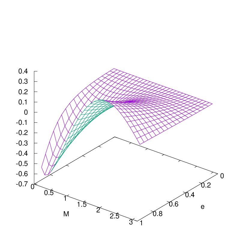
The error of this estimate relative to the accurate solution is shown in Figure 5. It increases where and .
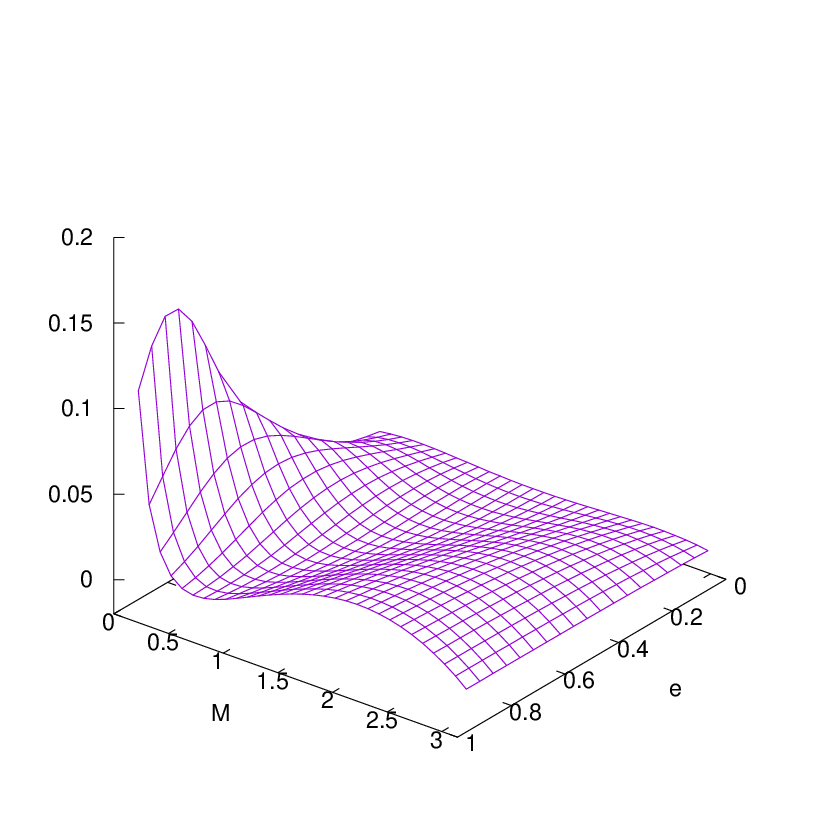
The figure shows that the (24) has the same benefit as (12) of approximating the solution from above, therefore converging Charles and Tatum 1997, but being more accurate. In consequence, the convergence is faster, as demonstrated in Figure 6 if compared with Figure 3.

III.5 Improved Inital Value, Version 2
If (3) is expressed as
| (25) |
both sides may be expanded in a Taylor series of ,
| (26) |
Keeping this series up to yields the estimate
| (27) |
This is basically the estimate of the second step of the fixed point iteration (7) with an enhancement factor of the second term if or are large. As pointed out earlier Danby and Burkardt 1983, this is also obtained applying the Newton method to the estimator .
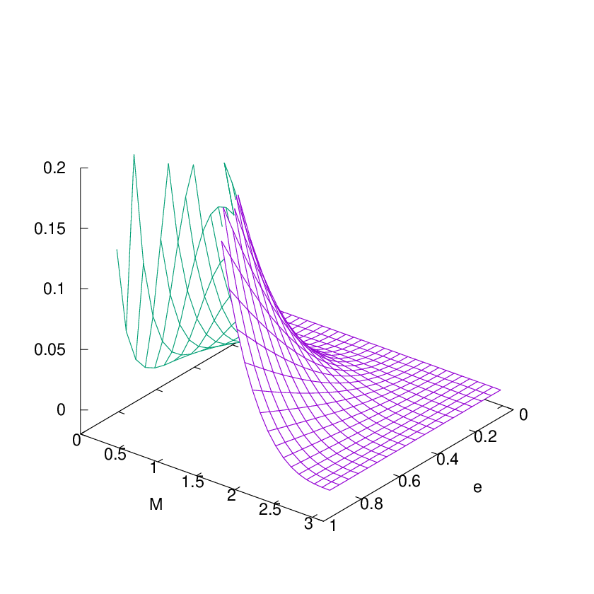
If the series is kept up to , the associated quadratic equation proposes
| (28) |
This quadratic equation is solved by
| (29) |
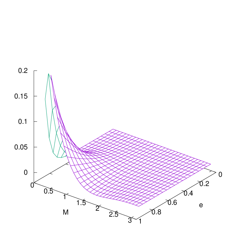
Figures 7 and 8 show in comparison with Figure 5 that these approximations derived from the Taylor series of are not better than the one from the quadratic estimate of .
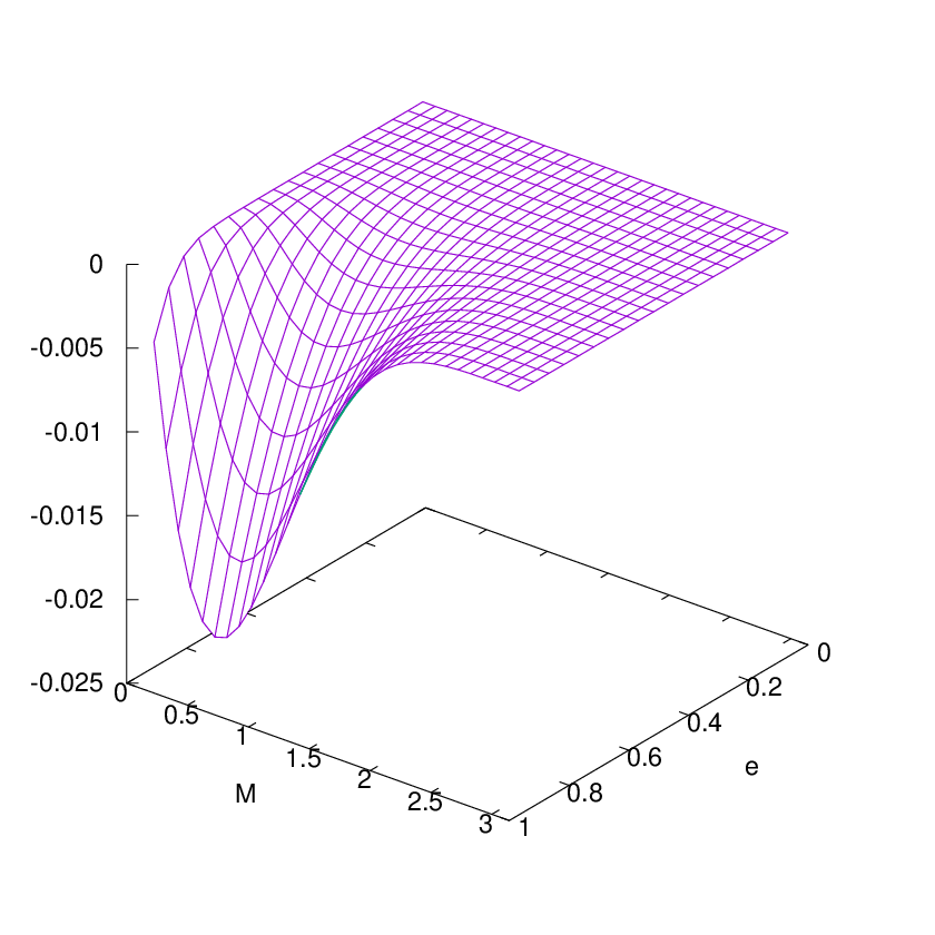
Expansion of (26) up to third order in yields a cubic equation for , which is even closer to the exact solution as demonstrated in Figure 9.
See Mikkola’s paper for a similar approach Mikkola 1987; Nijenhuis 1991; Markley 1995.
In a systematic treatment, (26) is power series of in powers of ,
| (30) |
with series inversion (Abramowitz and Stegun 1972, 3.6.25)
| (31) |
but this right hand side does not converge well for .
III.6 Adiabatic switching on
One principle in perturbative quantum mechanics switches on the fermionic interaction by increasing the coupling (fine structure) constant from zero (no interaction) up to the value attained by the real-world system. Adopting this concept here, the eccentricity is started at at the known solution , and the is tracked until the actual value of is reached. Let overdots denote partial derivatives with respect to at constant , e.g. , . The derivative of (2) is
| (32) |
| (33) |
To avoid numerically expensive evaluations of the trigonometric functions the auxiliary angle is introduced with derivative
| (34) |
Multiplying (33) with yields a nonlinear first order differential equation for ,
| (35) |
We solve this with a single-step “explicit” classic Runge-Kutta integration with the initial value up to the actual Zurmühl 1948; Butcher 1963. These estimates are surprisingly close to the actual solutions, as illustrated in Fig. 10.
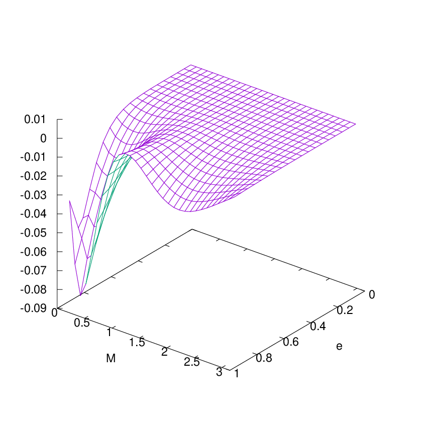
Fig. 11 demonstrates that 3 steps of the first-order Newton method suffice to obtain 12 digits accuracy in .
This approach is close in spirit to the Taylor series (6), but not suffering from the singularity at .

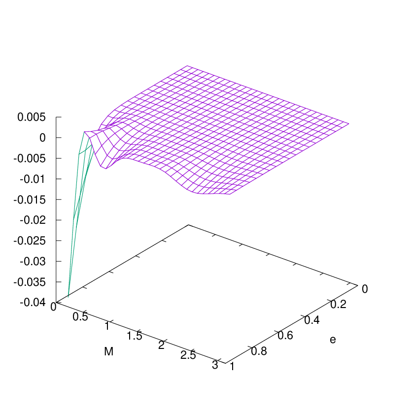
For higher accuracy we can also solve this with an “explicit” 5-th order Runge-Kutta-Fehlberg RK5(6) method, (Fehlberg 1968, Table III)(Fehlberg 1969, Tab. 1). The error in these guesses and the number of iterations in the Newton methods are summarized in Figures 12 and 13.

IV Summary
A initial value (24) combined with Halley’s equation (9) leads to fast and stable convergence for the inverse problem of Kepler’s equation for elliptic orbits. That initial value is simpler but generally worse than Markley’s estimator Markley 1995.
Appendix A C++ Implementation
A reference implementation is reprinted in the anc directory which implements (9) and (24). If compiled with the -DTEST preprocessor symbol, g++ -O2 -DTEST -o solveKepler solveKepler.cc, a test program is obtained which can be called with one option and two command line arguments, solveKepler [-1—-2—-3] , to investigate the convergence with this and other approaches. The option -1 indicates that iteration with (8) computes successive approximations, the option -2 (or none) indicates iteration with (9) and the option -3 iterations with Householder’s method including third derivatives Abbasbandy 2003. It prints for all implemented starting guesses the values of , , the index of the iteration loop in the Newton method, the estimate reached so far, and the error relative to the true solution.
The program switches over to solving
| (36) |
with the estimate for hyperbolic orbits if the command line parameter is larger than 1.
References
- Fitzpatrick (1970) P. M. Fitzpatrick, Principles of celestial mechanics (Academic Press, 1970).
- Danby and Burkardt (1983) J. M. A. Danby and T. M. Burkardt, The solution of kepler’s equation. i, Cel. Mech. 31, 95 (1983).
- Gerlach (1994) J. Gerlach, Accelerated convergence in Newton’s method, SIAM Review 36, 272 (1994).
- Hansen and Patrick (1977) E. Hansen and M. Patrick, A family of root finding methods, Numer. Math. 27, 257 (1977).
- Kalantari et al. (1997) B. Kalantari, I. Kalantari, and R. Zaare-Nahandi, A basic family of iteration functions for polynomial root finding and its characterizations, J. Comp. Appl. Math. 80, 209 (1997).
- Alefeld (1981) G. Alefeld, On the convergence of halley’s method, Am. Math. Monthly 88, 530 (1981).
- Esmaelzadeh and Ghadiri (2014) R. Esmaelzadeh and H. Ghadiri, Appropriate starter for solving the kepler’s equation, Int. J. Comp. Applic. 89, 31 (2014).
- International Astronomical Union (2023) International Astronomical Union, IAU SOFA Collection, Tech. Rep. (International Astronomical Union, 2023).
- Fukushima (1997) T. Fukushima, A method solving kepler’s equation without transcendental function evaluations, Cel. Mech. Dyn. Astr. 66, 309 (1997).
- Palacios (2002) M. Palacios, Kepler equation and accelerated newton method, J. Comp. Appl. Math 138, 335 (2002).
- Grau-Sánchez et al. (2011) M. Grau-Sánchez, A. Grau, and M. Noguera, Ostrowki type methods for solving systems of nonlinear equations, Appl. Math. Comput. 218, 2377 (2011).
- Chun (2007) C. Chun, Some variants of king’s fourth-order family of methods for nonlinear equations, Appl. Math. Comp. 190, 57 (2007).
- Conway (1986) B. A. Conway, An improved algorithm due to laguerre for the solution of kepler’s equation, in 24th Aerospace Sciences Meeting, 86-0083 (AIAA, 1986).
- Charles and Tatum (1997) E. D. Charles and J. B. Tatum, The convergence of newton-raphson iteration with kepler’s equation, Cel. Mech. Dyn. Astr. 69, 357 (1997).
- Stumpf (1999) L. Stumpf, Chaotic behaviour in the newton iterative function associated with kepler’s equation, Cel. Mech. Dyn. Astr. 74, 95 (1999).
- Abramowitz and Stegun (1972) M. Abramowitz and I. A. Stegun, eds., Handbook of Mathematical Functions, 9th ed. (Dover Publications, New York, 1972).
- Schonfelder (1980) J. L. Schonfelder, Very high accuracy Chebyshev expansions for the basic trigonometric functions, Math. Comp. 34, 237 (1980).
- Boyd (2007) J. P. Boyd, Rootfinding for a transcendental equation without a first guess: polynomialization of kepler’s equation through chebyshev polyomial expansion of the sine, Appl. Num. Math. 57, 12 (2007).
- Boyd (2009) J. P. Boyd, Chebyshev expansion in intervals with branch points with application to the root of kepler’s equation: A chebyshev-hermite-padé method, J. Comp. Appl. Math. 223, 693 (2009).
- Mikkola (1987) S. Mikkola, A cubic approximation for kepler’s equation, Cel. Mech. 40, 329 (1987).
- Nijenhuis (1991) A. Nijenhuis, Solving kepler’s equation with high efficiency and accuracy, Cel. Mech. Dyn. Astr. 51, 319 (1991).
- Markley (1995) F. L. Markley, Kepler equation solver, Cel. Mech. Dyn. Astr. 63, 101 (1995).
- Zurmühl (1948) R. Zurmühl, Runge-kutta-verfahren zur numerischen Integration von Differentialgleichungen n-ter Ordnung, Z. angew. Math. Mech. 28, 173 (1948).
- Butcher (1963) J. C. Butcher, Coefficients for the study of runge-kutta integration processes, J. Austral. Math. Soc. 3, 185 (1963).
- Fehlberg (1968) E. Fehlberg, Classical fifth-, sixth-, seventh-, and eigth-order runge-kutte formulas with stepsize control, (1968).
- Fehlberg (1969) E. Fehlberg, Klassische runge-kutte-formeln fünfter und siebenter ordnung mit schrittweiten-kontrolle, Computing 4, 93 (1969).
- Abbasbandy (2003) S. Abbasbandy, Improving newton-raphson method for nonlinear equations by modified adomian decomposition method, Appl. Math. Comput. 145, 887 (2003).