Differentiable Moving Horizon Estimation for Robust Flight Control
Abstract
Estimating and reacting to external disturbances is of fundamental importance for robust control of quadrotors. Existing estimators typically require significant tuning or training with a large amount of data, including the ground truth, to achieve satisfactory performance. This paper proposes a data-efficient differentiable moving horizon estimation (DMHE) algorithm that can automatically tune the MHE parameters online and also adapt to different scenarios. We achieve this by deriving the analytical gradient of the estimated trajectory from MHE with respect to the tuning parameters, enabling end-to-end learning for auto-tuning. Most interestingly, we show that the gradient can be calculated efficiently from a Kalman filter in a recursive form. Moreover, we develop a model-based policy gradient algorithm to learn the parameters directly from the trajectory tracking errors without the need for the ground truth. The proposed DMHE can be further embedded as a layer with other neural networks for joint optimization. Finally, we demonstrate the effectiveness of the proposed method via both simulation and experiments on quadrotors, where challenging scenarios such as sudden payload change and flying in downwash are examined.
I INTRODUCTION
Quadrotors are increasingly engaged in various challenging tasks such as flying in swarms [1] and transporting suspended payload with unknown weights [2]. The interaction with environments constantly generate complex forces and torques acting on quadrotors, such as those from the downwash [3], ground effects [4], wall effects [5], and the time-varying drag from a suspended payload [6], to name but a few. These disturbances affect the quadrotors’ dynamic behavior significantly and thus must be compensated appropriately for robust flight control.
Estimating and reacting to external disturbances has long been the focus of quadrotor research. The authors in [7] proposed a deep neural network (DNN) to learn the aerodynamic disturbance caused by the ground effect when landing quadrotors. A similar method has been further adapted to estimate multi-quadrotor interactions using permutation-invariant DNN [8]. Although these methods can predict the aerodynamic disturbances more accurately than some empirical models, they typically need the ground truth data for training, which is usually difficult to acquire and can only be estimated roughly. It is also difficult to generalize the method to multiple different scenarios due to the large volume of data needed for training. A unified estimation framework that is independent of the trajectory and controller was developed in [9] to estimate external forces and torques. However, the estimator requires the inputs to be carefully filtered since its design does not account for noise.
More recently, an extended-state Unscented Kalman Filter (UKF) was adopted in [10] for the disturbance estimation. The extended-state equations model the time-varying disturbance forces and torques as random walks. This method generally works well across different scenarios. However, its performance heavily depends on tens of noise variance parameters which are hard to identify in practice. The process of manually tuning these parameters is rather obscure and requires significant efforts and expert knowledge. To alleviate this tuning problem, [11] proposed an adaptive extended Kalman filter (EKF) that leverages an online expectation-maximization approach to estimate the predicted error covariance matrix, enabling it to be used in the case of unknown and time-varying noise covariance. However, the EKF lacks of robustness to the poor estimation of the noise covariance due to the linearization approximation.
Different from the above methods, we develop upon the moving horizon estimation (MHE) for the disturbance estimation. The MHE has been shown superior to UKF and EKF in terms of robustness, convergence rate, and estimation accuracy [12, 13]. In MHE, a finite horizon of the past state trajectory is estimated online by solving an optimization problem with the most current measurements. The objective function of MHE is a weighted summation of the so-called arrival cost and running cost. These weighting matrices are the tuning parameters of an MHE. They can be interpreted as the inverse of the noise variance matrices, the same as those assumed in a probabilistic filter such as UKF [14]. Similar to UKF, sophisticated tuning is required to achieve optimal performance.
This paper develops a data-efficient differentiable moving horizon estimation (DMHE) algorithm that can automatically tune its parameters online and is adaptive to different flight scenarios. To achieve this, we perform a sensitivity analysis by analytically computing the gradient of the MHE estimates with respect to (w.r.t) the tuning parameters. Specifically, it is derived by implicitly differentiating through the Karush-Kuhn-Tucker (KKT) conditions of the associated MHE optimization problem. The gradient enables us to train the tuning parameters using powerful machine learning techniques. More generally, it enables the embedding of MHE into neural networks for joint optimization. There has been a growing interest of joining the force of control-theoretic policies and machine learning techniques, such as OptNet [15], differentiable MPC [16] and Pontryagin differentiable programming [17]. Our work adds to this collection another general policy for estimation, which is of interdisciplinary interest to both the control and the machine learning community. Technical-wise, we construct an auxiliary MHE system to calculate the gradient more efficiently. Interestingly, we show that the auxiliary MHE can be solved very efficiently in a recursive form by leveraging a Kalman filter. Driven by the particular application, we also develop a model-based policy gradient algorithm to learn the tuning parameters directly from the quadrotor trajectory tracking error without the need for the ground truth.
Our main contributions are summarized in the following:
- 1.
We propose the auto-tuning DMHE, which is demonstrated to accurately estimate external disturbances acting on quadrotors such as sudden payload change, ground effect, and downwash effect;
- 2.
We develop an efficient method for training DMHE with gradient descent, which explores a recursive form using a Kalman filter;
- 3.
We develop a model-based policy gradient algorithm to learn the tuning parameters directly from the quadrotor trajectory tracking errors without the ground truth of the external disturbances;
- 4.
We demonstrate in simulation and experiment the joint optimization of NN-parameterized DMHE and control policy for robust flight control of quadrotors.
The rest of this paper is organized as follows. The quadrotor dynamics is presented in Section II. We derive the analytical gradient in Section III. Section IV presents the model-based policy gradient algorithm for learning the MHE without the ground truth data. Simulation and experiment results are reported in Section V and VI respectively. We discuss our future work and conclude the paper in Section VII.
II Preliminaries: Quadrotor Dynamics
We aim to improve the robustness of flight control of autonomous quadrotors by estimating and reacting to the external disturbances. The quadrotor is modeled as a 6 degree-of-freedom (DoF) rigid body with mass and moment of inertia . Define as the global position of CoM in inertial frame (North-East-Down), the velocity of CoM in , the rotational matrix from body frame to , and the angular velocity in , the dynamics of the quadrotor is given by:
| (1) | ||||
where disturbance forces and torques are expressed in and , respectively, is the gravitational constant, , denotes the skew-symmetric operator, is the control torques produced by the motor thrusts. We define as the quadrotor state and as the control wrench. Usually, the squared motor speeds are the control input of the quadrotor and linearly mapped to the control wrench by where is a 4-by-4 matrix defined by the aerodynamic coefficients and as well as the distance from each motor to center-of-mass (CoM) .
Common practice for robust control against disturbances is to estimate and compensate them in feedforward control. Next, based on the state-of-art estimator MHE, we develop algorithms of automatically tuning the MHE online to estimate the disturbances with fast dynamic response.
III Differentiable Moving Horizon Estimation
III-A MHE Formulation for Disturbance Estimation
Since the disturbance can be from arbitrary unknown sources, the most general way is to approximate them as random walks. This has proven to be very effective for estimating time-varying unknown disturbances [18, 10].
| (2) |
where and denote the process noises for the disturbance forces and torques, respectively. We then extend with to obtain . Both the rigid body dynamics (1) and the disturbance model (2) will be used in MHE for estimation.
Given the most recent measurements in a data window with a horizon of , the MHE estimates the trajectory of the extended state by solving the following optimization problem at each time step .
| (3) | ||||
where is the MHE estimate of at time , is the measurements at time , is the predicted output, is the discrete-time model for the extended system using 1st-order Euler method, , is sampling time, , , and are weight matrices. For brevity, we define the initial and terminal subscripts to be and , respectively, such that the estimate trajectory becomes .
We define a row vector as the tuning parameters that contain all the elements of those weight matrices, i.e. where is the vecterization operator. The first term in (3) approximates the arrival cost that summarizes the past data not explicitly accounted for in the cost [19]. We observe that increasing will slow down the dynamic response of MHE to the change of disturbance, but a very small will cause the MHE to be unstable. The second and third terms are a trade-off between the measurements and the model. If we are highly confident in the measurements based on a prior knowledge, then we increase relative to . Despite these rough intuitions, tuning to improve the estimate of disturbance can still be a quite tedious and intricate process.
The above intuitions indicate that the estimate trajectory is an implicit function of by solving the MHE problem. For a choice of , we refer to the problem (3) as and evaluate using a scalar differentiable loss . Our objective is to train such that the loss is minimized, which is cast as the following bilevel optimization problem.
| (4) |
III-B Analytical Gradient
We use gradient descent to solve the problem (4), which allows for tuning DMHE in end-to-end learning pipelines. The gradient of the loss with respect to is computed using the chain rule.
| (5) |
With (5), we illustrate the learning framework in Fig.1. Each update of involves a forward pass where given , is generated by solving MHE, and thus is formed, and a backward pass where and are computed.
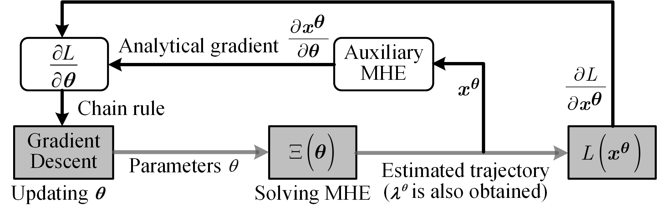
Since can be obtained by any nonlinear optimization solver, the main challenge is how to solve . Note that the gradient is also an implicit function of , which justifies the chain rule (5) for updating . Next, we will present an efficient way to compute the gradient analytically in a recursive form by proposing an auxiliary MHE system.
For the optimization problem (3) with a given , the KKT conditions define a set of necessary optimality conditions which must satisfy. We associate dual variable with the state constraints and the corresponding Lagrangian is thus formed as:
| (6) |
Let be the estimate of the current state, the data smooth based on the measurements , and the one-step model prediction. Therefore, the KKT conditions take the following form.
| (7a) | ||||
| with the boundary conditions: | ||||
| (7b) | ||||
where in the first equation of (7a), in the second and third equations of (7a), , , , and are the system matrices independent of . is because the terminal cost in the MHE is zero.
As mentioned before, our goal is to obtain . To this end, we define the following new state, new dual variables, and new process noise as:
| (8) |
In addition, the following matrices are also defined.
| (9) | ||||
The partial derivatives (9) and the system matrices can be easily obtained by any software that supports symbolic computation, e.g. CasADi [20]. By eliminating with in (7a) and using the above definitions (8) and (9), we can differentiate the KKT conditions (7a) and (7b) w.r.t , leading to the differential KKT conditions.
| (10) | ||||
where and .
Next, we will show that the differential KKT (10) can elegantly calculate the unknown matrix in (8) which proves to be exactly the output of an auxiliary MHE system of the following form.
| (11) | ||||
where denotes matrix trace. Interestingly, the auxiliary MHE (11) is linear and its cost function is quadratic. In addition, both the dynamics and solution of the system (11) are determined by the trajectory of the original MHE (3). Hence, we obtain the following important results.
Lemma 1
The proof is detailed in Appendix -A. Thanks to Lemma 1, we can obtain from efficiently using the following lemma.
Lemma 2
Given the initial condition:
| (12) | ||||
where is the identity matrix. The analytical solution of the auxiliary MHE system (11) can be obtained in the form of Kalman filter by leveraging dynamic programming [21], as below.
Kalman filter:
| (13a) | ||||
Backward update of dual variables:
| (13b) | ||||
Forward update of new state:
| (13c) |
The proof of Lemma 13c is presented in Appendix -B. We summarize the above procedures in Algorithm 1. The analytical gradient makes explicit use of a Kalman filter and has a recursive form. As such, it can be solved iteratively and is computationally efficient.
for to do 3
IV Model-based Policy Gradient
Given the analytical gradient (5), we propose a model-based policy gradient algorithm that learns the tuning parameters directly from the trajectory tracking errors, without the need for the ground truth. The algorithm is valid only when the quadrotor is under closed-loop control.
Suppose we have a general controller that takes the estimate of the quadrotor state as the feedback and accounts for the estimate of the disturbances .
| (14) |
where is reference trajectory. If the estimate trajectory from the MHE becomes more accurate, the tracking performance of the quadrotor under control should be improved. Otherwise, the quadrotor will deviate from the reference trajectory dramatically and even become unstable.
As such, we define the loss function for training as the weighted summation of the trajectory tracking errors over horizon which is the batch size.
| (15) |
where is a weight matrix for the tracking errors, and is the softmax weight related to .
We summarize the model-based policy gradient in Algorithm 2, in which is the mean loss of the training episode, is the learning rate, and is the duration for each episode.
for to do 2
Obtain using Algorithm 1;
Solve the control law (14);
Implement the control to obtain new state;
Obtain using (15);
Apply the chain rule (5) to obtain ;
Update end for 3
V Training in Simulation
This section presents the training results to validate that the model-based policy gradient algorithm can tune the MHE online to improve both the estimation and trajectory tracking performances directly from the trajectory tracking errors. In each training episode, the quadrotor under the geometric control [22] coupled with the DMHE will takeoff from the ground and follow a Lemniscate trajectory while being affected by various disturbances such as the ground effect, the square-wave and sinusoidal disturbances.


We introduce two forgetting factors in the weight matrices and , respectively, such that and . The weight matrices are assumed to be diagonal, in which case contains elements, i.e., where , , and . We set the initial values of the diagonal elements as and with four different initial conditions of as shown in Fig.2. The horizon is and the learning rate is different for different weight matrices, i.e., for , for , and for and . The parameters of the quadrotor are set as below: , , , and . We apply the line search algorithm to guarantee where the lower bound is tuned to be . The sampling time is and the quadrotor model (1) used in the simulation environment is discretized by 4th-order Runge Kutta method with the simulation step of . We code the simulation in Python and use ipopt as the solver in CasADi to implement optimization. The simulation is run in a PC with the processor of AMD Ryzen 9 5950X 16-Core.

Each episode lasts for , during which the quadrotor is controlled to track the reference trajectory (see Fig.2(b)) generated by the minimum snap algorithm [24]. We set the variance of measurement noise as , and the variance of process noise as . Fig.2(a) shows that the proposed algorithm is robust to different initial conditions and all the mean losses can converge to the same local minimum after training few episodes. Correspondingly, Fig.2(b) shows that the tracking performance in training is continuously improved, especially in z-direction. This is mainly due to the evident improvement in the disturbance force estimation (see Fig.2(c)). By comparison, the untrained DMHE responds slowly to the time-varying disturbances with large estimation bias and delay.
Note that the temporarily large tracking error during takeoff in the 1st training is caused by the initial increase of (see Fig.3, which begins at around 230 steps). This is due to the corresponding square-wave disturbances which subsequently lead to several impulse-like oscillations of . Despite this, can decrease and is eventually stable at around while increases to around . In addition, most of the elements in are less than those in , and the optimal significantly enlarge the difference between and . The trained weight matrices agree with the settings of the noise variances, implying that we have more confidence on the measurements than on the process.
We further test the algorithm complexity by measuring the running time needed for the whole algorithm 1 per iteration. Table.I summarizes the running time for different batch sizes. It is shown that the proposed algorithm 1 is computationally efficient as it can be run at high frequency.
| Horizon | |||||
|---|---|---|---|---|---|
| Running time |
VI Experimental Results
The experiments aim to demonstrate the ability of DMHE to train with controls and neural networks (NN) for joint optimization. This ability increases the potential of end-to-end learning for various scenarios. The control diagram is illustrated in Fig.4 where both and the control gains are modelled using two NNs. The proposed controller used in the experiments consists of a baseline controller (labelled as Controller in the Fig.4) and a NN-DMHE feedforward term for disturbance compensation. The baseline controller is a NN-parameterized Proportional-Derivative (NN-PD) controller with a gravity compensation. We evaluate the proposed controller in two experiments: 1) a step disturbance force by releasing a payload, and 2) a complex time-varying aerodynamic force by downwash effect. The setup of hardware platform required is outlined in Fig.5.


The training process is that the quadrotor with a payload tethered to it iteratively takes off. Similar to the disturbance defined in Section V, the payload mass is also a square-wave signal and its value is randomly set at the beginning. Since the force estimation and position dynamics are the primary concern in the experiment, consists of elements where are parameterized as, for example, . This parameterization is also applied to the control gains. As such, the outputs of two NNs are and ratio factors for and the control gains , respectively, and their inputs are the position and velocity feedback. Each NN consists of a hidden layer that contains neurons and takes PReLU as the activation function and an output layer with Sigmoid activation. Because only the estimate of the disturbance force is used in the controller, we modify the gradient of loss as in Eq.16 and formulate the loss for training the NN-DMHE as . The loss for training the NN-PD controller is formulated in a similar way as . We build and train the two NNs using PyTorch [25] and Adam [26] optimizer with and . After training episodes, the DMHE and controller parameterized by the two NNs are deployed to the real quadrotor without extra tuning.
| (16) |
where is the weighted summation of the tracking errors based on the feedback , is the discrete-time quadrotor position dynamics, i.e., , and is the estimate from the NN-DMHE.

Before the fly tests, we first use a payload of known weight () to calibrate the NN-DMHE to remove any bias caused by inaccurate modeling. The first experiment is to test the dynamic response of the NN-DMHE to a step-disturbance. To this end, we make the quadrotor take off with the payload and release it once hovering at the height setpoint. The payload is tethered to the quadrotor with tether length of . At around in Fig.6, the payload is released and the NN-DMHE responds to this sudden change quickly with a rising time less than . The external force posed by the payload (during about 10 to 20 s in Fig.6) is estimated by the NN-DMHE to be with a standard deviation of . This is a satisfactory estimation compared to the true weight of with the local gravitational acceleration at Singapore.


The second experiment is to test the robustness of the proposed method under the downwash effect. Passing through the downwash generated by another quadrotor can cause a significant loss of lift and thus lead to catastrophic failure. We program the ego quadrotor (see the setup in Fig.5) to automatically take off and hover at , and then let a second quadrotor hover at above the ego one (see Fig.7, which begins at around in Fig.8). We can see from Fig.8 that with the NN-DMHE, the ego quadrotor can maintain at the desired height after a mild oscillation with small amplitude. By comparison, Fig.8 shows that the baseline controller leads to a steady state tracking error before due to the ground effect and airflow interaction, and causes a severe oscillation after the downwash effect begins at . The steady error of about enlarges the distance between these two quadrotors but reduces the downwash effect, even in this case, the ego quadrotor under the baseline control still falls below the desired height for more than and fails to maintain the original height setpoint (having a static error of ). Fig.8 also shows that the second quadrotor under the PID control cannot maintain at the desired height setpoint above the ego one with a steady state tracking error of about due to the ceiling effect. Therefore, it is necessary to incorporate the NN-DMHE into the controller for providing the quadrotor with the robustness to these challenging disturbances. The downwash-induced time-varying disturbance force estimated by the NN-DMHE is plotted in Fig.9 for the -direction.
VII CONCLUSIONS
This paper proposes a data-efficient differentiable moving horizon estimation (DMHE) algorithm that can automatically tune the MHE parameters online to estimate the disturbances acting on quadrotors. At the core of our approach is the analytical gradient of the estimate trajectory of MHE w.r.t the tuning parameters, which enables auto-tuning by end-to-end learning. Simulation shows that a stable MHE with fast dynamic response can be learned directly from the trajectory tracking errors without the need for the ground truth by the proposed model-based policy gradient. Experiments validate the joint-optimization of the DMHE and NNs as well as control, which is adaptive to challenging scenarios such as sudden payload change and downwash effect.
Our future work will incorporate the DMHE into the simultaneous localization and mapping (SLAM) system in more challenging scenarios such as varying both disturbance forces and torques drastically. We believe the tightly coupled DMHE and SLAM system will further improve the robustness of the current quadrotor control and SLAM system.
References
- [1] W. Hönig, J. A. Preiss, T. S. Kumar, G. S. Sukhatme, and N. Ayanian, “Trajectory planning for quadrotor swarms,” IEEE Transactions on Robotics, vol. 34, no. 4, pp. 856–869, 2018.
- [2] S. Dai, T. Lee, and D. S. Bernstein, “Adaptive control of a quadrotor uav transporting a cable-suspended load with unknown mass,” in 53rd IEEE Conference on Decision and Control. IEEE, 2014, pp. 6149–6154.
- [3] N. Michael, D. Mellinger, Q. Lindsey, and V. Kumar, “The grasp multiple micro-uav testbed,” IEEE Robotics & Automation Magazine, vol. 17, no. 3, pp. 56–65, 2010.
- [4] C. Powers, D. Mellinger, A. Kushleyev, B. Kothmann, and V. Kumar, “Influence of aerodynamics and proximity effects in quadrotor flight,” in Experimental robotics. Springer, 2013, pp. 289–302.
- [5] Y. Naka and A. Kagami, “Coanda effect of a propeller airflow and its aerodynamic impact on the thrust,” Journal of Fluid Science and Technology, vol. 15, no. 3, pp. JFST0016–JFST0016, 2020.
- [6] S. Belkhale, R. Li, G. Kahn, R. McAllister, R. Calandra, and S. Levine, “Model-based meta-reinforcement learning for flight with suspended payloads,” IEEE Robotics and Automation Letters, vol. 6, no. 2, pp. 1471–1478, 2021.
- [7] G. Shi, X. Shi, M. O’Connell, R. Yu, K. Azizzadenesheli, A. Anandkumar, Y. Yue, and S.-J. Chung, “Neural lander: Stable drone landing control using learned dynamics,” in 2019 International Conference on Robotics and Automation (ICRA). IEEE, 2019, pp. 9784–9790.
- [8] G. Shi, W. Hönig, Y. Yue, and S.-J. Chung, “Neural-swarm: Decentralized close-proximity multirotor control using learned interactions,” in 2020 IEEE International Conference on Robotics and Automation (ICRA). IEEE, 2020, pp. 3241–3247.
- [9] T. Tomić and S. Haddadin, “A unified framework for external wrench estimation, interaction control and collision reflexes for flying robots,” in 2014 IEEE/RSJ International Conference on Intelligent Robots and Systems. IEEE, 2014, pp. 4197–4204.
- [10] C. D. McKinnon and A. P. Schoellig, “Estimating and reacting to forces and torques resulting from common aerodynamic disturbances acting on quadrotors,” Robotics and Autonomous Systems, vol. 123, p. 103314, 2020.
- [11] Y. Huang, Y. Zhang, B. Xu, Z. Wu, and J. A. Chambers, “A new adaptive extended kalman filter for cooperative localization,” IEEE Transactions on Aerospace and Electronic Systems, vol. 54, no. 1, pp. 353–368, 2017.
- [12] J. B. Rawlings and B. R. Bakshi, “Particle filtering and moving horizon estimation,” Computers & chemical engineering, vol. 30, no. 10-12, pp. 1529–1541, 2006.
- [13] W. Zhang, Z. Wang, C. Zou, L. Drugge, and M. Nybacka, “Advanced vehicle state monitoring: evaluating moving horizon estimators and unscented kalman filter,” IEEE Transactions on Vehicular Technology, vol. 68, no. 6, pp. 5430–5442, 2019.
- [14] T. Kraus, H. J. Ferreau, E. Kayacan, H. Ramon, J. De Baerdemaeker, M. Diehl, and W. Saeys, “Moving horizon estimation and nonlinear model predictive control for autonomous agricultural vehicles,” Computers and electronics in agriculture, vol. 98, pp. 25–33, 2013.
- [15] B. Amos and J. Z. Kolter, “OptNet: Differentiable optimization as a layer in neural networks,” in International Conference on Machine Learning. PMLR, 2017, pp. 136–145.
- [16] B. Amos, I. D. J. Rodriguez, J. Sacks, B. Boots, and J. Z. Kolter, “Differentiable mpc for end-to-end planning and control,” in Proceedings of the 32nd International Conference on Neural Information Processing Systems, 2018, pp. 8299–8310.
- [17] W. Jin, Z. Wang, Z. Yang, and S. Mou, “Pontryagin differentiable programming: An end-to-end learning and control framework,” Advances in Neural Information Processing Systems, vol. 33, 2020.
- [18] B. Yüksel, C. Secchi, H. H. Bülthoff, and A. Franchi, “A nonlinear force observer for quadrotors and application to physical interactive tasks,” in 2014 IEEE/ASME International Conference on Advanced Intelligent Mechatronics. IEEE, 2014, pp. 433–440.
- [19] C. V. Rao, J. B. Rawlings, and D. Q. Mayne, “Constrained state estimation for nonlinear discrete-time systems: Stability and moving horizon approximations,” IEEE transactions on automatic control, vol. 48, no. 2, pp. 246–258, 2003.
- [20] J. A. Andersson, J. Gillis, G. Horn, J. B. Rawlings, and M. Diehl, “Casadi: a software framework for nonlinear optimization and optimal control,” Mathematical Programming Computation, vol. 11, no. 1, pp. 1–36, 2019.
- [21] H. Cox, “Estimation of state variables for noisy dynamic systems,” Ph.D. dissertation, Massachusetts Institute of Technology, 1963.
- [22] T. Lee, M. Leok, and N. H. McClamroch, “Geometric tracking control of a quadrotor UAV on SE(3),” in 49th IEEE conference on decision and control (CDC). IEEE, 2010, pp. 5420–5425.
- [23] X. He, G. Kou, M. Calaf, and K. K. Leang, “In-ground-effect modeling and nonlinear-disturbance observer for multirotor unmanned aerial vehicle control,” Journal of Dynamic Systems, Measurement, and Control, vol. 141, no. 7, 2019.
- [24] D. Mellinger and V. Kumar, “Minimum snap trajectory generation and control for quadrotors,” in 2011 IEEE international conference on robotics and automation. IEEE, 2011, pp. 2520–2525.
- [25] A. Paszke, S. Gross, F. Massa, A. Lerer, J. Bradbury, G. Chanan, T. Killeen, Z. Lin, N. Gimelshein, L. Antiga et al., “Pytorch: An imperative style, high-performance deep learning library,” Advances in neural information processing systems, vol. 32, pp. 8026–8037, 2019.
- [26] D. P. Kingma and J. Ba, “Adam: A method for stochastic optimization,” arXiv preprint arXiv:1412.6980, 2014.
-A Proof for Lemma 1
The goal is to show that the KKT conditions of the auxiliary MHE system in (11) is exactly the differential KKT conditions defined in (10). For this purpose, we define the following Lagrangian for .
| (17) |
where denotes the dual variable for . The solution trajectory , together with the dual variable trajectory and the process noise trajectory , must satisfy the following KKT conditions.
| (18) | ||||
Comparing and the second sub-equation in Eq.(18) with gives the one of boundary conditions , which makes the above KKT conditions identical to the differential KKT in (10). This completes the proof.
-B Proof of Lemma 13c
The proof is by induction. It is to prove that the relation also holds at time . Then, by the differential KKT (10), we have
| (19) |
Replacing with the solution in (13c) leads to
| (20) |
According to the differential KKT in (10), the dual variable at time should satisfy the following equation.
| (21) |
Plugging the above equation into (20) gives:
| (22) | ||||
Add and subtract in right-hand-side and then collect all in left-hand-side:
| (23) | ||||
Finally, the Kalman filter (13a) gives the desired result as:
| (24) |
The initial condition is obtained by setting , in which case as it is the last dual variable. Substituting into (10) and using the same manipulation method as (23) can yield the desired initial condition (12). This, together with the above equations, completes the proof.