A Bayesian inference and model selection algorithm with an optimisation scheme to infer the model noise power2015A Bayesian inference and model selection algorithm with an optimisation scheme to infer the model noise power–References
Abstract
Model fitting is possibly the most extended problem in science. Classical approaches include the use of least-squares fitting procedures and maximum likelihood methods to estimate the value of the parameters in the model. However, in recent years, Bayesian inference tools have gained traction. Usually, Markov chain Monte Carlo methods are applied to inference problems, but they present some disadvantages, particularly when comparing different models fitted to the same dataset. Other Bayesian methods can deal with this issue in a natural and effective way. We have implemented an importance sampling algorithm adapted to Bayesian inference problems in which the power of the noise in the observations is not known a priori. The main advantage of importance sampling is that the model evidence can be derived directly from the so-called importance weights – while MCMC methods demand considerable postprocessing. The use of our adaptive target, adaptive importance sampling (ATAIS) method is shown by inferring, on the one hand, the parameters of a simulated flaring event which includes a damped oscillation and, on the other hand, real data from the Kepler mission. ATAIS includes a novel automatic adaptation of the target distribution. It automatically estimates the variance of the noise in the model. ATAIS admits parallelisation, which decreases the computational run-times notably. We compare our method against a nested sampling method within a model selection problem.
Keywords:
methods: statistical – methods: numerical – methods: data analysis – stars: activity – stars: flare1 Introduction
Bayesian data analysis has become a popular tool in many research fields. A particular type of problem in which Bayesian analysis is often used consists in fitting models to empirical data in order to estimate the value of their unknown parameters. This is referred to as Bayesian inference. Two different methods are commonly applied in Bayesian inference: Markov chain Monte Carlo (MCMC) and importance sampling (IS). In the Astrophysical literature, it is common to find applications of various MCMC algorithms (see Caruso et al. 2019; Komanduri et al. 2020; Martinez et al. 2020, for some recent examples). Contrarily, IS methods are rarely used to infer parameters (Wraith et al. 2009; Lewis & Bridle 2011), but to determine the Bayesian evidence with the accepted samples from an MCMC-based method (Perrakis et al. 2014; Nelson et al. 2016, e.g.).
One reason for the popularity of MCMC methods is that they are easy to implement. However, MCMC methods present some significant disadvantages. A well-known problem is that they generate correlated samples (Martino, L., & Elvira, V. 2017), although different methods may be applied to mitigate this problem (Pascoe et al. 2020, e.g.). In addition, MCMC algorithms are difficult to parallelise (although different chains can be run in parallel). However, the main disadvantage of MCMC is its difficulty for determining the model evidence (a.k.a. marginal likelihood) directly and, hence, comparing different models for the same dataset. A solution for that problem is proposed by Green 1995, where the author presents a method to create reversible Markov chain samplers that jump between models with different dimensionality. In recent years, MCMC methods have been applied extensively in exoplanet searches. Some examples are Gregory 2011, Barros et al. 2016, Affer et al. 2019, and Trifonov et al. 2019, among many others. A list of research groups working on this issue can be found in Dumusque et al. 2017 and in Nelson et al. 2020. MCMC are also used in spectroscopic studies (Greene et al. 2018; Casasayas-Barris et al. 2020).
Compared to MCMC methods, IS techniques offer a simpler and much more natural solution to the problem of model selection, as they readily yield estimates of the model evidence without additional computations. Moreover, IS algorithms admit simple parallelisation and they can be combined with MCMC methods to permit larger coverage of the state space (Martino 2018). Besides, “the IS methods are elegant, theoretically sound, simple-to-understand, and widely applicable” (Bugallo et al. 2017). Several of these methods are available in the specialised literature (Cappé et al. 2004; Cornuet et al. 2012; Elvira et al. 2015) and most of them involve some kind of adaptation for the mean and variance of the proposal distribution (Martino et al. 2017). Like MCMC, IS methods admit tempering or annealing schemes (Swendsen & Wang 1986). The power of the IS methods resides in the capability of inferring the model parameters together with the marginal likelihood.
Distinct methods to compute the marginal likelihood are available in the literature (see Llorente et al. 2021, for an extensive review). These can be classified into four families. A first class of methods are those based on deterministic approximations and density estimation, like the Bayesian-Schwarz information criterium (Schwarz 1978, BIC;). Under some, sometimes weak assumption, these methods approach the Bayes factor or they estimate the value of the posterior density, around previously chosen samples. The samples are obtained using some sampling method like acceptance-rejection (ARM), MCMC or others. The second family corresponds to the techniques based on IS. They draw samples from one or more proposal distribution and determine weights for them. These weights can be used to approximate the marginal posterior directly without additional computations (Elvira et al. 2017). A third class of methods are those based on the joint use of MCMC and IS. They combine the capability of MCMC methods to explore the parameter/state space and that of IS to approximate the marginal posterior (Perrakis et al. 2014; Nelson et al. 2016; Martino 2018). The last family of methods are based on quadrature schemes. They are settled on the Lebesgue representation of the integral of the marginal likelihood (Llorente et al. 2021). The most often used of them is the so-called nested sampling (see Buchner 2021a, for a complete review). Nested sampling (NS) is a method developed specifically for the problem of model selection (Skilling 2006). Nevertheless, currently most available codes incorporate a bayesian inference algorithm (Speagle 2020; Buchner 2021b). In practice, NS estimates the marginal likelihood by quadratures through the use of nodes. These nodes are particular samples drawn with a sampling method, commonly MCMC (Feroz et al. 2019).
A good example of a model selection problem in astrophysics is exoplanet detection through radial velocity curves. Inference must be performed on the five parameters defining the planet’s orbit. In addition, a sixth parameter is needed to account for the mean radial velocity of the star. For each planet additionally included in the model, another five parameters need to be inferred. Hence, the number of dimensions grows rapidly and models must be compared by means of the marginal likelihoods. In addition, the statistics of the observational noise are not known a priori and inference on them is not easy. Several attempts have been made in the past to introduce IS for exoplanet search. Loredo et al. 2011 developed an adaptive IS (AIS) method to estimate the marginal likelihood to compare between models with planets and without planets. However, that is still an open line of research. Previously, Hogg et al. 2010 had applied IS to infer the distribution of the planet’s eccentricity. The authors indicate that the method can be applied to any other model parameter. Finally, Liu 2014 proposed an AIS method with annealing to explore the marginal posterior pdfs. In any case, the problem of estimating the actual power of the noise affecting the observations is not tackled.
Another example of a process with many parameters to infer is flaring events that trigger plasma oscillation (Mathioudakis et al. 2006; Nakariakov & Stepanov 2007; Stepanov et al. 2012; Reale 2016; López-Santiago et al. 2016; López-Santiago 2018; Nakariakov & Kolotkov 2020, e.g). Here, the distinct models represent different decay functions of the oscillation and the flare intensity in the observed light curve (Pascoe et al. 2020). A minimum of eight parameters are needed for an exponentially damped oscillation with constant background. The number of model parameters increases rapidly if a non uniform background or multi exponential decay are included.
In this work, we present an implementation of an IS scheme for model inference that includes adaptation and weight clipping (Koblents & Miguez 2015). We also incorporate a novel target adaptation procedure. The method is termed ATAIS. A formal statistical study of the adaptation procedure, including its performance and comparison with actual marginal posteriors from a multimodal distribution was carried out in Martino et al. 2021. The details of the method together with theoretical aspects are explained in the next sections. They include several algorithms to implement the method in the reader preferred programming language. The main advantage of ATAIS with respect to other AIS methods is that it incorporates an optimisation procedure to determine the power of the observation noise automatically. This optimisation scheme avoids the use of annealing and the need to infer the variance of the noise together with the remaining model parameters. After running of ATAIS, the posterior distribution of the noise variance is obtained as explained in Section 5 of Martino et al. 2021. Furthermore, a global bayesian evidence can be determined that includes the noise variance as a parameter instead of fixing it.
This article is structured as follows. Bayesian model fitting is briefly introduced in Section 2. Section 3 shows a formal, brief description of the IS method. Its application to Bayesian inference problems is described in Section 4, together with a generic algorithm. Section 5 describes the new ATAIS algorithm, an IS scheme with adaptation of the proposal distribution including a procedure to infer the variance of the noise. Section 6 presents an application of the method for model selection. The accuracy of the results is compared with that of nested sampling methods. An application of the method to detect and characterise a damped oscillation in a flare light curve is presented in Section 7.1. Conclusions are given in Section 8.
2 Bayesian approach to model fitting
Consider a physical process described by a certain model. The latter depends on one or more unknown parameters that have to be inferred by fitting the model to empirical data . Commonly, observations are affected by noise, which we assume additive. Therefore, we can write
| (1) |
where is a random vector that follows a probability distribution with zero mean and covariance matrix ( denotes the identity matrix) and is the transformation that maps the model parameters into the space of the observations. Usually, the noise power parameter, hereby denoted by is not known and must be inferred too. Let be the set of parameters to be inferred, which includes the noise power, i.e.
| (2) |
where is the number of parameters in the model.
From a Bayesian perspective, is a set of random variables. Its posterior probability density function (pdf) given the data can be written by applying the Bayes’ theorem, as
| (3) |
where is the so-called likelihood function (the pdf of the data conditional on the set of parameters ), is the prior distribution of (encoding the prior knowledge about the parameters) and is the model (or Bayesian) evidence11 1 We use an argument-wise notation for pdfs where, given two random variables and , and are the pdfs of and , respectively, and they are possibly different functions. Moreover, denotes the join pdf of the pair and is the conditional pdf of given .. Note that is an unnormalised posterior function, i.e., a function proportional to . Generally, in real world applications, we are able to evaluate (point-wise) the function instead of because the normalising constant
| (4) |
cannot be computed. The minimum mean square error (MMSE) estimator of is (Pearson 1894)
| (5) |
where is the parameter space. To be specific, this estimator coincides with the conditional expectation of the random parameter vector given the available observations –hence, we denote . Other classic estimators which are often used are the maximum a posteriori (MAP) estimator,
| (6) |
or the median of the posterior distribution, . None of these point-wise estimators, , , , can be computed analytically in most real world scenarios. Furthermore, interval estimations are often required in order to provide uncertainty analysis and outlier detection, for instance. Approximations of the posterior distribution, , and related integrals are required to compute all these quantities.
One approach to the approximation of the posterior distribution is the use of Monte Carlo (MC) algorithms. They provide a sample-based approximation of the posterior (with a random support) that can be obtained virtually for any kind of posterior distribution and any dimension of the inference space. The obtained population of samples can be employed to approximate integrals involving the posterior distribution. One important family of MC methods are the so-called Markov Chain Monte Carlo algorithms. Another important family of MC methods are the Importance Sampling (IS) techniques. There are several advantages in using IS with respect to MCMC (as mentioned in Section 1). One clear benefit of IS is the ability to approximate the model evidence with an easy-to-implement estimator. Estimation of the model evidence via MCMC requires much more sophisticated and, in general, less efficient methods. The main disadvantage is that they tend to be less efficient in exploring the parameter space.
3 Brief introduction to importance sampling (IS)
Let us assume that we are interested in obtaining the expected value of a random variable , denoted . If the variable follows a distribution with pdf , its expected value is given by the integral
| (7) |
The subindex indicates that the expectation is under . The integral is over the entire space of the variable, . For instance, if is a unidimensional real variable, then . The integral in Eq. (7) may not have an analytical solution. The Monte Carlo approximation (Metropolis & Ulam 1949) consists in drawing samples from the density function so that
| (8) |
Often, it is hard to draw samples from directly. In such case, an auxiliary pdf, known as proposal function and denoted by , can be used to rewrite the expectation in Eq. (7) as
| (9a) | ||||
| (9b) | ||||
| (9c) | ||||
The last integral in Eq. (9) is the expected value of the function under , which we denote as . We have shown, therefore, that . We can further elaborate on this expression to arrive at
| (10a) | ||||
| (10b) | ||||
where it has been used that is a pdf and, therefore, . From Eq. (10), we readily obtain the Monte Carlo approximation,
| (11) |
where
| (12) |
are normalised weights and the ’s are samples from . The method is called importance sampling, and the ’s are referred to as importance weights (Robert & Casella 2005).
4 Application to Bayesian inference
From Eq. 7, the MMSE estimator of given the data is the conditional expectation
| (13) |
Equation 8 provides an approximation to this integral if enough samples are drawn from . However, the posterior distribution of is usually hard to sample. Importance sampling is simple to apply, though. Using the method outlined in Section 3, we obtain
| (14a) | ||||
| (14b) | ||||
| (14c) | ||||
| (14d) | ||||
| (14e) | ||||
where . The term is usually referred to as the target function (or unnormalised posterior distribution). A standard Monte Carlo approximation now yields
| (15) |
where , , and is the number of samples. An alternative estimator (that avoids the need to compute ) is obtained by normalising the weights , namely
| (16) |
where
| (17) |
are normalised importance weights. Similarly, an estimate of the covariance matrix is
| (18) |
Equations (16)-(18) are used when the model evidence is unknown and they provide a method for approximating the expected value of a parameter, or a set of parameters in the model, together with their covariance matrix and any other statistics that may be of interest. Note also that estimates of and can be easily obtained using the set of weighted samples. For instance, is given by .
4.1 Estimation of the model evidence
A great advantage of using importance sampling is that the model evidence can be estimated directly from the individual weights of each Monte Carlo sample . As a result, a comparison between models can be easily done (while other methods, like MCMC, require post-processing (Ford & Gregory 2007; Perrakis et al. 2014; Nelson et al. 2016; Pascoe et al. 2020). From Eq. (3),
| (19) |
but we can rewrite this integral using the importance pdf as
| (20a) | ||||
| (20b) | ||||
| (20c) | ||||
| (20d) | ||||
Then, using a standard Monte Carlo approximation,
| (21) |
This is the arithmetic mean of the unnormalised importance weights. It is important to remark that Eq. (21) is only valid if is normalised.
4.2 Summary of the importance sampling algorithm
The method is summarised in Algorithm 1 (Rubin 1987).
The set of weighted samples enables us to approximate posterior expectations of the form
for any integrable function . In particular, it is straightforward to construct the weighted-mean estimator
| (22) |
and it can be proved, under mild assumptions, that (see, e.g., Robert & Casella 2005).
- Choose a proposal density, .
/* Sampling: */
5 Adaptive Target Adaptive Importance Sampling (ATAIS)
5.1 Adaptive Importance Sampling
The generic algorithm described in Section 4 works fine when the dimension of is not high. If the number of parameters to infer is large enough, IS may fail in estimating the expected value of or obtaining its approximated posterior distribution. The reason is that those samples drawn from the proposal distribution may not cover the parameter space correctly. In high-dimensional problems, a large number of samples might be required to get accurate results. A solution to this issue is to repeat the process after adapting the proposal using the information given by the importance weights (see Bugallo et al. 2017, for an extensive review). This iterative process is called Adaptive Importance Sampling (Oh & Berger 1992, AIS;).
There exist many procedures for adapting the proposal in AIS (Cappé et al. 2004; Cornuet et al. 2012; Elvira et al. 2015; Martino et al. 2017). The standard scheme consists in updating the mean and variance of the proposal distribution with the mean and variance from Eqs. 16 and 18. A classic alternative is to replace the mean by the maximum a posteriori . This is the set of parameters that maximises the target distribution . For symmetric posterior distributions like multivariate gaussians, is equal to the expected value . However, this does not hold for asymmetric or multimodal distributions. The choice of or depends on the problem. When the target distribution is multimodal, for instance, the use of leads to more samples tracing the highest mode, which might leave the remaining ones poorly identified or even missing. Instead, the use of will probably sample all the modes but it may need many iterations to obtain a good representation of each single mode. Algorithm 2 provides pseudocode for a general implementation of AIS.
/* Iterations: */
The final estimators of a generic AIS algorithm can be expressed as
| (23) |
| (24) |
5.2 Weight clipping
Algorithm 2 can be enhanced using different techniques. A convenient modification of AIS that is useful for high-dimensional problems is the so-called weight clipping (Koblents & Miguez 2015; Míguez et al. 2018). A usual problem when working with AIS is the degeneracy of the importance weights due to the curse of dimensionality (Bengtsson et al. 2008, see). If the number of parameters to be inferred and/or the space to be explored are large, it is difficult to reach regions of the state space with high probability density during the first iterations. As a result, all or most of the samples drawn from the proposal will have null weight. Therefore, the adaptation will be done with only one sample or very few samples, which makes the method inefficient. A solution to this problem is to select a fixed number of samples with the largest weights and assign all of them the same weight. The expected value and the variance of the samples are determined using the new weights and the adaptation is modified consequently. The resulting scheme preserves the convergence properties of classical IS while mitigating the weight degeneracy problem.
5.3 AIS with adaptive target
In Bayesian inference, it is common to deal with noisy data. The lack of precise information about the power of this noise conditions the results of the inference method, since an incorrect choice of this parameter may hamper the convergence of the algorithm. Inferring both the set of parameters entering the map and the noise power is difficult. We propose a method to optimise the value of while inferring the parameters using AIS.
As mentioned in Section 2, the map is a function of the parameters , such that
| (25) |
where is the -parameter space. If the perturbation noise is assumed to follow a normal distribution,
| (26) |
where is the noise power. Then, the likelihood function is
| (27) |
Note that we have two types of variables of interest: the vector contains the parameters of the nonlinear map , whereas is a scale parameter of the likelihood function. In our approach, AIS is used to infer the values of , while is adapted at each iteration according to the quadratic difference of the best fit. The latter is given by the approximate MAP estimator, (see Algorithm 3).
| (28) |
Note that needs to be initialised at step and it is updated only if (where is the variance at the step ). Therefore, corresponds to a minimum square error (MSE). An outline of the method with multivariate Gaussian proposals is given in Algorithm 3. Empirical results show that it is always convenient to start with a large value of .
6 Model selection with ATAIS
We include here an example that demonstrates the capability of ATAIS in accurately computing the marginal likelihood within a model selection problem. ATAIS results are compared with those obtained by numerically integrating the marginal likelihood using a dense grid. In addition, we compare ATAIS with nested sampling methods. For this purpose, we have chosen UltraNest (Buchner 2021b), an implementation of a rigorous nested sampling method. For the sake of reproducibility, we have used the example described in the UltraNest tutorial22 2 The code can be downloaded from the UltraNest GitHub page (https://johannesbuchner.github.io/UltraNest/example-sine-modelcomparison.html).. The problem consists in computing the marginal likelihood for a given dataset using two distinct models. The first model () is,
| (29) |
The second model () is a one dimensional sinusoid,
| (30) |
In both models represents white, gaussian noise. The dataset consists of 50 points randomly selected between and from model (meaning M1 is the true model). The model parameters are fixed to for the baseline of the signal, for the amplitude, for the period and for the phase. The variance of the noise is set to .
6.1 Comparison with numerical integration of the marginal likelihood
For the numerical integration, the parameter space has been divided into cells of uniform width 0.1 for , and , and 0.02 for . The limits of the integral are the same as the boundaries of the prior pdfs defined in the UltraNest tutorial example: , , , and . We have applied an expensive trapezoidal rule for the integration in order to obtain the ground-truth values. The marginal likelihood computed33 3 The values of listed in the text have been obtained by using the likelihood function defined in the example of the UltraNest tutorial (). For a normalised Gaussian likelihood function, we obtain and . for the model is , while we obtain for . With these values, the Bayes factor . Therefore, the preferred model with the uniform priors defined in this example is , despite the data having been generated with the model . Actually, this result is not surprising. The signal-to-noise ratio of the data is low since the amplitude of the sinusoid () used to generate the data is lower than the standard deviation of the noise. Note that the marginal likelihood tends to penalise models with high complexity.
We have applied ATAIS to the simulated dataset. We have iterated the algorithm 20 times, each one with samples, for a total of samples in the single run. The prior pdfs defined here are uniform, with the same ranges in the parameter space than those used for the numerical integration. The proposal pdf of each model parameter is assumed normal with initial variance . The initial mean of each proposal pdf has been chosen randomly from the corresponding prior pdf. The run has been completed in 5.8 seconds in a 2.3 GHz Quad-Core Intel Core i5 processor. With this configuration for ATAIS, we have obtained , and . Therefore, ATAIS approximates correctly the true values of the marginal likelihood (see above the results of expensive trapezoidal integration). No substantial difference is found in these values with distinct runs of ATAIS.
ATAIS performs inference over the model parameters and the noise variance (). Eventually, a marginal likelihood can be computed for different values of (). The later is done by sampling from a prior and applying Eqs. 24 and 25 in Martino et al. 2021. Figure 1 shows a corner plot of the marginal posteriors and pairwise correlations for the model . The parameters inferred by ATAIS are shown at the top of each histogram, together with the 90% credibility interval. In this example, they correspond to the MAP estimators. Hereafter, we use instead of . The algorithm converges to for this model. The variation of the marginal likelihood with the value of the variance for the model () is shown in Figure 3. Similarly, Figure 2 shows the marginal posterior pdf of the constant in the model . For this model, the algorithm converges to . The variation of the marginal likelihood with the variance for this model () is also shown in Figure 3.


6.2 Comparison with nested sampling
The marginal likelihoods computed by UltraNest for the dataset and models used in the previous section are and . Thus, the Bayes factor is .44 4 There is a slight mistake in the UltraNest tutorial. The prior for the parameter is defined between 1 and 100, instead of 0.3 and 30 as indicated in the comment line. We have corrected it for our test. With this result, the preferred model is . Note that the prior pdfs defined for the parameters and in the tutorial are uniform in a logarithmic scale. As a consequence, the estimation of the marginal likelihood is different from that computed using the numerical integration with a uniform grid. The algorithm yields this result when 400 live points (or nodes) are used. The total number of evaluations of the likelihood for the model is .
For the comparison with ATAIS, we have defined the same prior pdfs with the model . Like in the previous section, the proposal pdf of each model parameter is assumed normal with initial variance . We have obtained , while the marginal likelihood of remains the same than in the previous section (). Therefore, the Bayes factor is . Like with UltraNest, the preferred model with these prior pdfs is . The results with ATAIS are in agreement with those obtained using UltraNest. The difference between UltraNest and ATAIS results is likely due to the way that ATAIS deals with the noise variance, which in UltraNest is fixed.
The inferred values for the four parameters of using the log-uniform priors for and are similar to those obtained in the previous section. Their corresponding marginal posteriors are shown in the diagonal of Figure 4. The values on top of those marginal posteriors are the estimates of the parameters. The lower and upper limits are the 90% credibility intervals. The algorithm converges to for this model. This value is similar to that obtained in the previous section. Our results show that the ATAIS scheme is robust and that the inference is not dependent of the prior pdfs provided the correct values are not excluded.

7 An application of ATAIS for bayesian inference: flare light curves
7.1 Simulated data of a flare with oscillation
The performance of our method for Bayesian inference and model selection is tested against simulated data of a flare light curve with a damped oscillation. The use of simulated data permits to control the sources of error in a way that it is not possible with real data. We assume the flare emission is governed by a short exponential rise phase followed by a longer exponential decay. The rise phase is modelled by
| (31) |
Here, is a vector of time instants, is a constant related to the flare amplitude, is the rise time and is the time of the peak emission. The decay phase is represented by
| (32) |
where is the decay time. The oscillation is modelled by the sinusoid
| (33) |
where is the amplitude of the oscillation, is its period and its starting time. Finally, the oscillation is exponentially damped by
| (34) |
The combination of Eqs. 31 to 34 is a generic model for the flare light curve with an oscillation,
| (35) |
Therefore, the model contains eight parameters to be inferred,
| (36) |
For the simulations, we have used the values listed in Table 1. For simplicity, we have considered gaussian white noise. The variance of this noise has been fixed to (in flux units). Figure 5 shows the simulated light curve. Note that the algorithm does not require prior information about units in the model. Therefore, we do not include them in the figure or the table.
| 72 | 30.2 | 5 | 30 | 20 | 9 | 24 | 40 |
|---|

We propose two alternatives for model testing. The first alternative is a model of several flares (each with an exponential rise and decay phases) that account for a process of repetitive ignition of different loops. The second alternative is the model of a single flaring loop with a damped oscillation described previously. Our main goal is to perform inference on the parameters of the two models. Additionally, we estimate the model evidence (Eq. 21) for each model and compare them using ATAIS. To check whether the algorithm is able to distinguish between the correct model and a multi-loop model with many parameters, we have assumed up to three flaring loops in the multiple flares model. The model with two flaring loops contains eight parameters to infer, like the model of a single loop with an oscillation. The model with three flaring loops has 12 different parameters. Hereafter, we will denote by the model of the single flare with oscillation and and the models with two and three flares without oscillation, respectively.

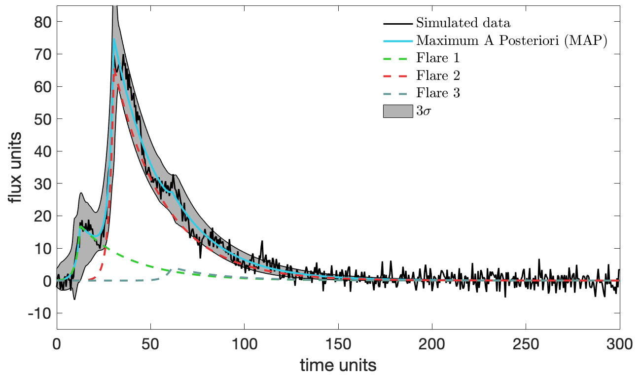
Our algorithm has been run for each model using samples and iterations, for a total of generated samples. The prior pdfs for each model are shown in Table 2. The results of the inference are summarised in Figures 6 and 7. The former corresponds to the model of a single flaring loop with a damped oscillation (). The latter shows the results for the multi-flare model with three flaring loops (). The multi-flare model with two loops does not reproduce correctly any of the bumps in the simulated data beyond and it is not considered here. In both figures, the continuous (cyan) line is the light curve generated with the maximum a posteriori (MAP) estimate and the grey area is the envelope generated with the samples of every iteration of the algorithm. At first glance, the two models seem to fit correctly the data. However, the estimations of the marginal likelihood of the two models give preference to the model of a single flare and damped oscillation (). It is important to note that the value of the marginal likelihood depends on the selection of the prior pdfs. Different pdfs will result in a different Bayes factor. Another indication that the preferred model is is the value of obtained by ATAIS. While for , we obtain , for the algorithm converges to . Here, has units of squared flux in this example. Table 3 shows the value of the parameters inferred for model with the confidence interval. The coincidence with the values used for the simulation (Table 1) is noticeable.
| Parameter | Prior |
|---|---|
| Model | |
| Model | |
| Model | |
| 72.66 | 30.30 | 4.93 | 29.16 | 26.24 | 8.94 | 24.07 | 29.17 |
7.2 Real data: white light flare
To conclude with the tests, we include an example with real data from a white-light flare observed with Kepler and analysed by Pascoe et al. 2020. These authors use a Bayesian inference tool developed specifically for analysing flare light curves (Anfinogentov et al. 2021, the Solar Bayesian Analysis Tool, SoBAT;). SoBAT contains an MCMC algorithm for inference and an importance sampling algorithm to determine the marginal likelihood of the data and perform model selection. Pascoe et al. 2020 analyse several white light flares in their article. Here, we focus on the data of the star KIC 12156549. The results of Pascoe et al. 2020 are discussed in their Section 3.2. The authors do not include the prior pdfs for all the parameters in their models, nor they show the expectations for the inferred values. In addition, the implementation of each one of their models contains one dimension more than our implementation, which corresponds to the observed noise variance. As a result, we cannot compare our estimations directly with theirs. However, we can compare the estimation of the noise variance that the authors obtained for each model, which is included in their Figures 6 and 8.
For the comparison, we have implemented the multi-flare model with two and four flares, together with the type P oscillation model with spline envelope. All those models are described in detail in Pascoe et al. 2020 and we do not reproduce them here. The prior pdfs for the peak time of the distinct flares are given in Section 3.2 of that work and those of their amplitudes, rise and decay times are indicated in their Section 2. For the oscillatory signal, we use uniform prior pdfs defined by the intervals [0, 400], [200, 400] and [0, 400] for the amplitude, starting time and period, respectively. Note that the starting time interval is chosen such that the oscillation would be triggered by the second flare, as suggested by Pascoe et al. 2020. For the spline envelope, we use three points with the initial time coincident with the oscillation starting time, and the interpolating and last point as free parameters. Their uniform priors are defined in the interval [0, 400] and [400, 600]. The value of the interpolating point has a uniform prior pdf in the interval [0, 10]. Summarising, we compare three different models with dimensions , and , respectively.
Our results are shown in Figure 8. They have been obtained after 10 iterations with samples per iteration, for a total of samples. The multi-flare model with two flares does not reproduce the observed light curve correctly, like in Pascoe et al. 2020 and we do not show the result here. The noise standard deviation determined from ATAIS for the four flares model is . For the model with the oscillation, we obtain . These values are similar to those obtained by Pascoe et al. 2020. With the prior pdfs previously defined, the estimations of the marginal likelihood of the two models give preference to the multi-flare model with four flares () against the model with two flares and an oscillation (), . Although this result is similar to that of Pascoe et al. 2020, the values of the marginal likelihood are not comparable because the authors do not give information for every prior pdf in their oscillation model.


8 Summary and conclusions
In this work, we present an implementation of the adaptive importance sampling method with adaptation of the target (ATAIS) developed in Martino et al. 2021. The method accepts different adaptation schemes and includes weight clipping to avoid the so-called weight degeneracy problem of importance sampling. We remark that the use of weight clipping is not mandatory but it is recommended for high-dimensional problems to avoid the weight collapse, i.e., that only one significant sample is used at each iteration. The main advantage of ATAIS with respect to MCMC methods is that the model evidence can be determined directly from the importance weights. This makes the comparison between different models (with the same data) easier. Compared to other adaptive importance sampling (AIS) methods, ATAIS includes a target adaptation scheme that uses the mean square error (MSE) in the current iteration to modify the variance of the likelihood function. With this optimisation scheme, the intensity of the noise is inferred, together with the model parameters. This noise includes not only observational errors but that of model selection/truncation.
The performance of the ATAIS algorithm is tested against simulated and real data. First, we demonstrate the capability of ATAIS to accurately compute the marginal likelihood within a model selection problem in Section 6. The simulation is from a sinusoid with very low signal-to-noise ratio. The two models confronted are the sinusoid model and a pure noise model. ATAIS results are compared with those of a numerical integration of the marginal likelihood and with a novel nested sampling method. ATAIS is able to accurately reproduce the marginal likelihood determined with the numerical integration for both models. Its performance is similar to that of nested sampling schemes. We then use ATAIS for a bayesian inference problem for higher dimension models. In this test, we simulate the light curve for a single loop flare with an exponentially damped oscillation. In addition, we use our algorithm to analyse real data from a flare detected with the space mission Kepler. Our results are compared with those obtained by Pascoe et al. 2020 with a combination of MCMC and IS methods. The results are discussed in Section 7. The method is able to discriminate between different models including oscillations and multi-flare models by comparing their model evidences. The latter are outcomes from the method. For the case of real data, our results are similar to those obtained by Pascoe et al. 2020. ATAIS is a powerful tool for Bayesian inference problems. It is meant for model selection problems where the number of unknown parameters varies across the candidate models. For example, in the comparison of models with different numbers of planets or the distinct models of ignition of flaring events in solar type stars as those analysed in Section 7. ATAIS is also appealing if the model noise is not known a priori. This method includes an optimisation scheme to determine the noise variance. No tempering schemes, of the type commonly used in MCMC methods, are needed. Neither is inferring the noise variance as yet another parameter, thereby increasing the dimension of the model.
Acknowledgements
This work was supported by the Office of Naval Research (N00014-19-1-2226), Spanish Ministry of Science and Innovation (CLARA; RTI2018-099655-B-I00) and Regional Ministry of Education and Research for the Community of Madrid (PRACTICO; Y2018/TCS-4705). This paper includes data collected by the Kepler mission and obtained from the MAST data archive at the Space Telescope Science Institute (STScI). Funding for the Kepler mission is provided by the NASA Science Mission Directorate. STScI is operated by the Association of Universities for Research in Astronomy, Inc., under NASA contract NAS 5–26555. The authors acknowledges fruitful discussion with the referee to improve the manuscript.
Data Availability
The simulated data underlying this article will be shared on reasonable request to the corresponding author. The algorithms developed for this work are coded in Matlab55 5 https://www.mathworks.com/products/matlab.html. They will be shared on reasonable request to the corresponding author.
References
- Affer et al. (2019) Affer L., et al., 2019, A&A, 622, A193
- Anfinogentov et al. (2021) Anfinogentov S. A., Nakariakov V. M., Pascoe D. J., Goddard C. R., 2021, ApJS, 252, 11
- Barros et al. (2016) Barros S. C. C., et al., 2016, A&A, 593, A113
- Bengtsson et al. (2008) Bengtsson T., Bickel P., Li B., 2008, Curse-of-dimensionality revisited: Collapse of the particle filter in very large scale systems. Institute of Mathematical Statistics, Beachwood, Ohio, USA, pp 316–334, doi:10.1214/193940307000000518, https://doi.org/10.1214/193940307000000518
- Buchner (2021a) Buchner J., 2021a, arXiv e-prints, p. arXiv:2101.09675
- Buchner (2021b) Buchner J., 2021b, The Journal of Open Source Software, 6, 3001
- Bugallo et al. (2017) Bugallo M. F., Elvira V., Martino L., Luengo D., Miguez J., Djuric P. M., 2017, IEEE Signal Processing Magazine, 34, 60
- Cappé et al. (2004) Cappé O., Guillin A., Marin J. M., Robert C. P., 2004, Journal of Computational and Graphical Statistics, 13, 907
- Caruso et al. (2019) Caruso D., Haardt F., Fumagalli M., Cantalupo S., 2019, MNRAS, 482, 2833
- Casasayas-Barris et al. (2020) Casasayas-Barris N., et al., 2020, A&A, 635, A206
- Cornuet et al. (2012) Cornuet J.-M., Marin J.-M., Mira A., Robert C. P., 2012, Scandinavian Journal of Statistics, 39, 798
- Dumusque et al. (2017) Dumusque X., et al., 2017, A&A, 598, A133
- Elvira et al. (2015) Elvira V., Martino L., Luengo D., Corander J., 2015, in 2015 IEEE International Conference on acoustics, speech, and Signal Processing (ICASSP). International Conference on Acoustics Speech and Signal Processing ICASSP. IEEE, pp 4075–4079
- Elvira et al. (2017) Elvira V., Martino L., Luengo D., Bugallo M. F., 2017, Signal Processing, 131, 77
- Feroz et al. (2019) Feroz F., Hobson M. P., Cameron E., Pettitt A. N., 2019, The Open Journal of Astrophysics, 2, 10
- Ford & Gregory (2007) Ford E. B., Gregory P. C., 2007, in Babu G. J., Feigelson E. D., eds, Astronomical Society of the Pacific Conference Series Vol. 371, Statistical Challenges in Modern Astronomy IV. p. 189 (arXiv:astro-ph/0608328)
- Green (1995) Green P. J., 1995, Biometrika, 82, 711
- Greene et al. (2018) Greene T. P., Gully-Santiago M. A., Barsony M., 2018, ApJ, 862, 85
- Gregory (2011) Gregory P. C., 2011, MNRAS, 415, 2523
- Hogg et al. (2010) Hogg D. W., Myers A. D., Bovy J., 2010, ApJ, 725, 2166
- Koblents & Miguez (2015) Koblents E., Miguez J., 2015, Statistics and Computing, 25, 407
- Komanduri et al. (2020) Komanduri A., Banerjee I., Banerjee A., Sengupta S., 2020, MNRAS, 499, 5690
- Lewis & Bridle (2011) Lewis A., Bridle S., 2011, CosmoMC: Cosmological MonteCarlo (ascl:1106.025)
- Liu (2014) Liu B., 2014, The Astrophysical Journal Supplement Series, 213, 1
- Llorente et al. (2021) Llorente F., Martino L., Delgado D., Lopez-Santiago J., 2021, preprint arXiv:2005.08334
- López-Santiago (2018) López-Santiago J., 2018, Philosophical Transactions of the Royal Society of London Series A, 376, 20170253
- López-Santiago et al. (2016) López-Santiago J., Crespo-Chacón I., Flaccomio E., Sciortino S., Micela G., Reale F., 2016, A&A, 590, A7
- Loredo et al. (2011) Loredo T. J., Berger J. O., Chernoff D. F., Clyde M. A., Liu B., 2011, arXiv e-prints, p. arXiv:1108.0020
- Martinez et al. (2020) Martinez L., Bersten M. C., Anderson J. P., González-Gaitán S., Förster F., Folatelli G., 2020, A&A, 642, A143
- Martino (2018) Martino L., 2018, Digital Signal Processing, 75, 134
- Martino, L., & Elvira, V. (2017) Martino, L., & Elvira, V. 2017, Wiley StatsRef: Statistics Reference Online, p. arXiv:1704.04629
- Martino et al. (2017) Martino L., Elvira V., Luengo D., Corander J., 2017, Statistics and Computing, 27, 599
- Martino et al. (2021) Martino L., Llorente F., Cuberlo E., López-Santiago J., Míguez J., 2021, Mathematics, 9
- Mathioudakis et al. (2006) Mathioudakis M., Bloomfield D. S., Jess D. B., Dhillon V. S., Marsh T. R., 2006, A&A, 456, 323
- Metropolis & Ulam (1949) Metropolis N., Ulam S., 1949, J. Am. Stat. Assoc., 44, 335
- Míguez et al. (2018) Míguez J., Mariño I. P., Vázquez M. A., 2018, Signal Processing, 142, 281
- Nakariakov & Kolotkov (2020) Nakariakov V. M., Kolotkov D. Y., 2020, ARA&A, 58, 441
- Nakariakov & Stepanov (2007) Nakariakov V. M., Stepanov A. V., 2007, Quasi-periodic Pulsations as a Diagnostic Tool for Coronal Plasma Parameters. p. 221
- Nelson et al. (2016) Nelson B. E., Robertson P. M., Payne M. J., Pritchard S. M., Deck K. M., Ford E. B., Wright J. T., Isaacson H. T., 2016, MNRAS, 455, 2484
- Nelson et al. (2020) Nelson B. E., et al., 2020, AJ, 159, 73
- Oh & Berger (1992) Oh M.-S., Berger J. O., 1992, Journal of Statistical Computation and Simulation, 41, 143
- Pascoe et al. (2020) Pascoe D. J., Smyrli A., Van Doorsselaere T., Broomhall A. M., 2020, ApJ, 905, 70
- Pearson (1894) Pearson K., 1894, Philosophical Transactions of the Royal Society of London Series A, 185, 71
- Perrakis et al. (2014) Perrakis K., Ntzoufras I., Tsionas E. G., 2014, Computational Statistics & Data Analysis, 77, 54–69
- Reale (2016) Reale F., 2016, ApJ, 826, L20
- Robert & Casella (2005) Robert C. P., Casella G., 2005, Monte Carlo Statistical Methods (Springer Texts in Statistics). Springer-Verlag, Berlin, Heidelberg
- Rubin (1987) Rubin D. B., 1987, Journal of the American Statistical Association, 82, 543
- Schwarz (1978) Schwarz G., 1978, The Annals of Statistics, 6, 461
- Skilling (2006) Skilling J., 2006, Bayesian Analysis, 1, 833
- Speagle (2020) Speagle J. S., 2020, MNRAS, 493, 3132
- Stepanov et al. (2012) Stepanov A., Zaitsev V., Nakariakov V., 2012, Coronal Seismology: Waves and Oscillations in Stellar Coronae. Wiley, https://books.google.es/books?id=Dz4ynohPgW4C
- Swendsen & Wang (1986) Swendsen R. H., Wang J.-S., 1986, Phys. Rev. Lett., 57, 2607
- Trifonov et al. (2019) Trifonov T., et al., 2019, AJ, 157, 93
- Wraith et al. (2009) Wraith D., Kilbinger M., Benabed K., Cappé O., Cardoso J.-F., Fort G., Prunet S., Robert C. P., 2009, Phys. Rev. D, 80, 023507